First SDO AIA Observations of a Global Coronal EUV “Wave”: Multiple Components and “Ripples”

Abstract

We present the first SDO AIA observations of a global coronal EUV disturbance (so-called “EIT wave”) revealed in unprecedented detail. The disturbance observed on 2010 April 8 exhibits two components: one diffuse pulse superimposed on which are multiple sharp fronts that have slow and fast components. The disturbance originates in front of erupting coronal loops and some sharp fronts undergo accelerations, both effects implying that the disturbance is driven by a CME. The diffuse pulse, propagating at a uniform velocity of 204–$238\mathrm{\,km}\mathrm{\,s}^{-1}$ with very little angular dependence within its extent in the south, maintains its coherence and stable profile for $\sim$30 minutes. Its arrival at increasing distances coincides with the onsets of loop expansions and the slow sharp front. The fast sharp front overtakes the slow front, producing multiple “ripples” and steepening the local pulse, and both fronts propagate independently afterwards. This behavior resembles the nature of real waves. Unexpectedly, the amplitude and FWHM of the diffuse pulse decrease linearly with distance. A hybrid model, combining both wave and non-wave components, can explain many, but not all, of the observations. Discoveries of the two-component fronts and multiple ripples were made possible for the first time thanks to AIA’s high cadences ($\leq$20 s) and high signal-to-noise ratio.

1. Introduction

Expanding annular, global-scale, coronal EUV enhancements were discovered with SOHO EIT and have been often called “EIT waves” (Moses et al., 1997; Thompson et al., 1998). They propagate across the solar disk at typical velocities of 200–$400\mathrm{\,km}\mathrm{\,s}^{-1}$ (Thompson & Myers, 2009), slower than Moreton (1960) waves ($\sim$1000 $\mathrm{\,km}\mathrm{\,s}^{-1}$). Their nature is still under intense debate. Competing models include: fast-mode MHD waves (Wills-Davey & Thompson, 1999; Wang, 2000; Wu et al., 2001; Warmuth et al., 2001; Ofman & Thompson, 2002; Schmidt & Ofman, 2010), slow-mode waves or solitons (Wills-Davey et al., 2007; Wang et al., 2009), and non-waves related to a current shell or successive restructuring of field lines at the CME front (Delannée, 2000; Chen et al., 2002, 2005; Attrill et al., 2007; Attrill, 2010). Details of observations and models can be found in recent reviews (Warmuth, 2007; Vršnak & Cliver, 2008; Wills-Davey & Attrill, 2009; Gallagher & Long, 2010).

Major drawbacks that hindered our understanding of such propagating EUV disturbances were EIT’s single view point and low cadence ($\geq$12 minutes), which were partially alleviated by STEREO EUVI (Long et al., 2008; Veronig et al., 2008; Ma et al., 2009; Kienreich et al., 2009; Patsourakos & Vourlidas, 2009). The Atmospheric Imaging Assembly (AIA) on the Solar Dynamics Observatory (SDO) has 10 EUV and UV wavelengths, covering a wide range of temperatures, at high cadence (up to 10–20 s, $\sim$$10\times$ faster than STEREO’s 75–150 s) and resolution ($1\farcs 4$, with $0\farcs 6$ pixels). These capabilities allow us to study the kinematics and thermal structure of EUV disturbances in unprecedented detail, as reported in this Letter.

2. Observations and Data Analysis

The event of interest (Solar Object Locator: SOL2010-04-08T02:30:00L177C061) occurred in NOAA active region (AR) 11060 (N25E16) from 02:30 to 04:30 UT on 2010 April 8. It involved a GOES B3.8 two-ribbon flare, CME, and global EUV disturbance, as shown in Figure 1. No Moreton wave was found in available H$\alpha$ data (from the Huairou Solar Observing Station, China).

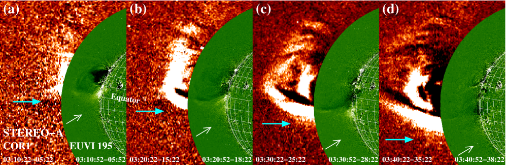
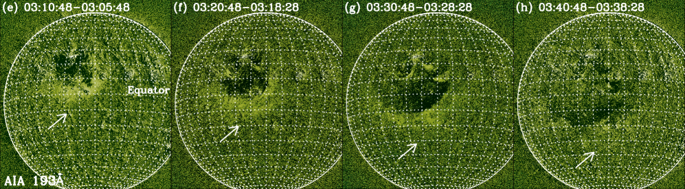
Figure 1.— Running difference images of composite STEREO-A COR1 and EUVI 195 Å (top, see online Movie 1) and AIA 193 Å (bottom), where the ecliptic and solar norths are up, respectively. Heliographic grids are spaced by $10^{\circ}$. Arrows point to the leading front of the diffuse pulse seen in whitelight and EUV. The cyan arrows are also approximately the projection of AIA’s line-of-sight (LOS; in the ecliptic plane) seen by STEREO-A.

AIA images (20 s cadence) were first coaligned across wavelengths and differentially rotated to a reference time (03:33:47 UT). Figure 2 shows selected images. To minimize human subjectivity, we employed a semi-automatic approach (cf., Wills-Davey, 2006), following Podladchikova & Berghmans (2005). We identified the eruption center (flare kernel centroid at $x=-238\arcsec$, $y=487\arcsec$) as the new “north pole”, and drew $15^{\circ}$ wide heliographic “longitude” sectors (A0–A11, Figures 2(a)–(b)). For each sector, we obtained the image profile as a function of distance measured from the eruption center along “longitudinal” great circles (thus correcting for the atmosphere’s sphericity) by averaging pixels in the “latitudinal” direction. Composing such 1D profiles over time gives a 2D space-time plot, from which base and running ratios and differences (giving different color scaling suited for different features) can be readily obtained, as shown in Figures 3 and 5.

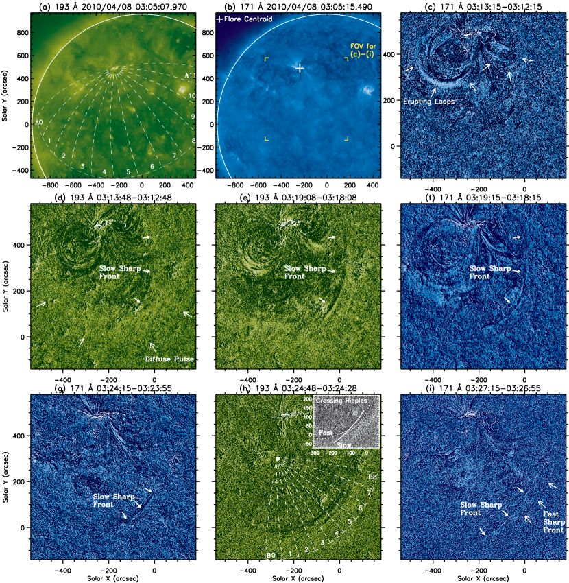
Figure 2.— Sequential AIA images at 193 and 171 Å: (a)–(b) original (see online Movies 2a–b) and (c)–(i) running difference (Movies 2c–d), with two field of views (FOVs). Overlaid are two sets of spherical sectors, A0–A11 in (a) and B0–B8 in (h), used to obtain space-time plots. The insert in (h) highlights multiple ripples.

The global disturbance is visible in all seven AIA EUV channels and for the first time observed at 131, 94, 335, and 211 Å. It is similar in channels $>$1 MK, being the strongest at 193 and 211 Å. It appears different in the cooler 171 Å channel and the weakest at 304 and 131 Å. Here we focus on the representative 193 and 171 Å channels (hereafter 193 and 171). Incidentally, we noticed very fast (500–$1200\mathrm{\,km}\mathrm{\,s}^{-1}$), narrow-angle features launched southward from the erupting AR, repeatedly at $\sim$100 s intervals throughout a 1.5 hrs duration, even after the global disturbance had left. Their nature is under investigation and will be presented in the future.

3. Erupting Loops and CME

Figure 3.— Running ratio space-time plots obtained from A sectors shown in Figure 2(a) at 193 (top) and 171 (bottom), smoothed with a 60 s boxcar. In (c) and (d), cross signs connected by dotted lines mark linear fits to the peak of the diffuse pulse at 193, with the fitted velocities printed on the top. Their end points are repeated in the corresponding 171 panels at the bottom. Other dotted lines are parabolic (linear in Figure 5) fits to various features, with the greater of the initial and final velocities listed on the left in the order of the start time of the fit (marked by an open circle). Fits in (e) are repeated in (a). Movie 3 shows this figure with and without labels and fits.

There is initially a series of coronal loops, best seen at 171, fanning out along an arcade in the northwest-southeast direction. At the flare onset of 02:32 UT, these loops, as shown in Figure 2(c), start to expand southward to the quiet Sun, likely avoiding the probably stronger magnetic field of large scale loops in the north (see Movies 2a–b). This first occurs in the inner core of the AR and successively proceeds to surrounding loops. The expansion experiences a gradual and then rapid acceleration. Parabolic fits to its space-time position (Figure 3(e)) before and after 03:11 UT yield accelerations of $26\pm 1$ and $94\pm 5\mathrm{\,m}\mathrm{\,s}^{-2}$ and final velocities of $52\pm 3$ and $234\pm 13\mathrm{\,km}\mathrm{\,s}^{-1}$, close to the 286 $\mathrm{\,km}\mathrm{\,s}^{-1}$ velocity of the halo CME measured by SOHO LASCO. STEREO Ahead, $67^{\circ}$ east of the Earth, observes this event at near quadrature and indicates that the lateral expansion of the CME is also primarily toward the south (Figure 1, top; Movie 1). The similar velocities and common direction suggest that the erupting loops are part of the CME body.

4. Global EUV Disturbance

4.1. Overview

The global EUV disturbance, seen by AIA on the solar disk, exhibits two components: one broad, diffuse pulse superimposed on which are multiple narrow, sharp fronts (see Movies 2c–d). The diffuse pulse appears as an annular-shaped emission enhancement ahead of the erupting loops. It expands in all directions except to the north, being the strongest in the southwest (Figure 1, bottom; Figure 2(d)). The sharp fronts also have two components: a slow front that appears earlier and occupies from the west to southwest of the AR (Figures 2(d)–(g)), and a fast front that comes later near the peak location of the diffuse pulse and dominates from southwest to south (Figures 2(h)–(i)).

In running ratio space-time plots at 193 (Figure 3, top), the diffuse pulse appears as a diagonal stripe of emission increase (bright) followed by decrease (dark), the boundary between which corresponds to the pulse peak. In Sector A4, for example, the peak coincides with the fast sharp front and propagates up to $800\arcsec$ (580 Mm) from the flare kernel. At 171 (Figure 3, bottom), the pulse is less pronounced and, in contrast, appears as emission reduction (dark followed by bright; Wills-Davey & Thompson, 1999; Dai et al., 2010) rather than commonly observed enhancement (e.g., Long et al., 2008). Together, these observations suggest that the cooler 171 material is heated to 193 temperatures.

The side view from STEREO-A indicates that the diffuse EUV enhancement is confined in the low corona and its leading front matches the lateral extent of the whitelight CME (Patsourakos & Vourlidas, 2009; Kienreich et al., 2009). It is followed by an arc-shaped sharp increase and then decrease of emission that extends into the COR1 FOV (high corona). Its projection onto the disk likely corresponds to the diffuse pulse’s peak and/or one of the sharp fronts seen by AIA, according to its latitudinal position, sharpness, and large vertical extent (thus large LOS integration).

4.2. Diffuse Pulse Shape Evolution

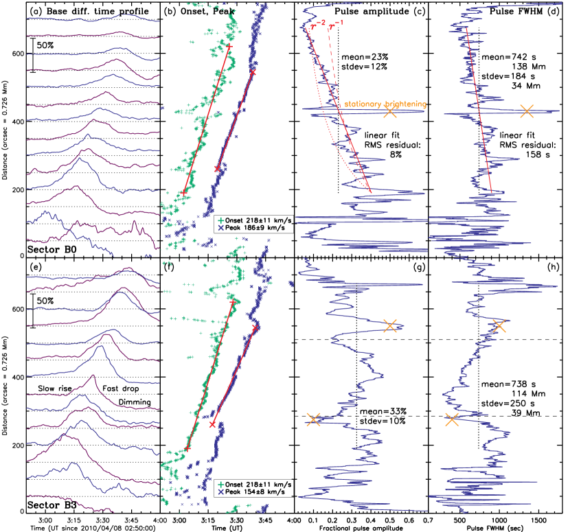
Figure 4.— Top: (a) Horizontal cuts of the normalized 193 base difference space-time plot of Sector B0 shown in Figure 2(h). Each curve represents the percentage emission variation at a fixed location marked by the dotted line (also representing the pre-event level). (b)–(d) Distance vs. onset and peak times, amplitude, and FWHM of the pulse shown in (a). The red solid lines are linear fits, and the red dashed and dotted lines in (c) are $r^{-1}$ and $r^{-2}$ fits starting with the same value at $s=190\arcsec$. Vertical dotted lines mark the mean values in the distance range of interest. The orange “$\times$”s in (c)–(d) indicate stationary brightenings of small scale loops. Bottom: same as Top but for Sector B3.

To best track the strong disturbance in the southwest, we used a finer set of $10^{\circ}$ wide sectors (B0–B8, Figure 2(h)) centered at $x=-275\arcsec$, $y=306\arcsec$, which are approximately perpendicular to the local disturbance front (to which the A sectors are not).

For selected Sectors B0 and B3, we composed base difference space-time plots, normalized by their average pre-event brightness. We then obtained time profiles from horizontal slices at every distance of the space-time plot. As shown in Figures 4(a) and (e) for 193, the profiles represent net emission changes and clearly show a single hump successively delayed with distance, corresponding to the propagating diffuse pulse. We define the pulse onset at the 20% level between the peak and the pre-event minimum, from which the pulse amplitude and FWHM are calculated. Note that these temporal profiles at fixed locations are equivalent to spatial profiles at given times (i.e., vertical slices of space-time plots), because the pulse is fairly stable and propagates at constant velocities (see Section 4.3).

In B0, where the slow sharp front is absent, the diffuse pulse clearly develops beyond $s_{0}=190\arcsec$ ($370\arcsec$ south of the flare kernel), within which it is not well-defined. The pulse amplitude can be fitted with a linear function, which decreases with distance by a fraction of ${6\over 7}$ from a 41% enhancement at $s_{0}$ to 6% at $675\arcsec$ (Figure 4(c)). (For comparison, the corresponding maximum emission reduction at 171 is only $\sim$10%.) It decreases faster than the corresponding $r^{-1}$ fit but slower than $r^{-2}$, implying the pulse being neither a surface nor a spherical wave. The pulse FWHM decreases by only ${1\over 3}$ from 902 to 581 s (Figure 4(d)), rather than increases as expected from dispersion of a wave.

In B3, where the fast and slow sharp fronts overlap (see Movie 4b), the pulse shape is quite different. Despite complications caused by stationary brightenings or dimmings of small-scale loops, an increase followed by a decrease of the pulse amplitude is roughly anti-correlated with variations of the FWHM in the distance range marked by the dashed lines (Figures 4(g)–(h)). This indicates steepening and then broadening of the pulse. The narrowest pulse (near $s=350\arcsec$) shows a sharp drop and deep, long-lasting dimming on its trailing edge, which are different from leading edge steepening in shock formations.

4.3. Kinematics of Disturbance Propagation

We derive kinematics of the disturbance propagation from base and running ratio space-time plots for B sectors as shown in Figure 5.

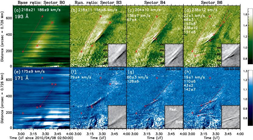
Figure 5.— Same as Figure 3 but for base (column 1) and running (columns 2–4) ratios from B sectors shown in Figure 2(h). Plus (cross) signs connected by dotted lines are linear fits to the onset (peak) of the diffuse pulse. Their end points for 193 are repeated for 171 at the bottom. The color bars on the right are for column 1 only, while columns 2–4 share the color scales with Figure 3. The gray scale inserts provide enlarged views showing parallel and crossing ripples. (See online Movies 4a–c for this figure and running difference images from which the space-time plots are obtained.)

4.3.1 Diffuse Pulse

At 193 (Figures 4(b) & (f) and 5(a)–(d)), both the onset and peak of the diffuse pulse travel at constant velocities in their mid stages, with the former being slightly faster (e.g., $218\pm 21$ vs. $186\pm 9\mathrm{\,km}\mathrm{\,s}^{-1}$ for Sector B0). This, despite the lack of a general trend for the overall pulse FWHM noted above, indicates that the rising portion of the pulse broadens at increasing distances in all directions, consistent with that found by Veronig et al. (2010). In addition, the pulse onset velocity weakly depends on directions, with a narrow range of $204$–$238\,\mathrm{\,km}\mathrm{\,s}^{-1}$.

At 171 (Figures 5(e)–(h)), with the signal being considerably weaker, the maximum emission reduction of the diffuse pulse propagates at similar velocities as its 193 counterpart of emission enhancement, e.g., $175\pm 9$ vs. $186\pm 9\mathrm{\,km}\mathrm{\,s}^{-1}$ for Sector B0. There is a delay by $\sim$230 s in time or $\sim$42 Mm in space, which we speculate could result from different wavelength response to the convolution of temperature and density effects, both being likely present here.

4.3.2 Sharp Fronts

At 193, the sharp fronts are recognized as narrow ridges in running ratio space-time plots (Figures 5(b)–(d)), and some of them experience acceleration (e.g., Figure 5(d)). Their final velocities in different directions vary by a factor of two ($136$–$238\mathrm{\,km}\mathrm{\,s}^{-1}$), in contrast to the narrow range of the diffuse pulse’s onset velocity.

At 171 (Figure 5, bottom), most of the sharp fronts are emission enhancements, opposite to the diffuse pulse reduction, but the same as their 193 counterparts at similar velocities (e.g., $128\pm 6$ vs. $136\pm 7\mathrm{\,km}\mathrm{\,s}^{-1}$ for B4). This suggests a density increase at both channels’ temperatures. The slow sharp front here is particularly pronounced and dominant over the fast front (see Figures 5(f)–(h), inserts). Its velocity is only $\sim$50% that of the diffuse pulse’s peak (e.g., $79\pm 4$ vs. $154\pm 8\mathrm{\,km}\mathrm{\,s}^{-1}$ for B3) and decreases toward the west, giving rise to its southward elongated oval shape (Figure 2(f)).

Incidentally, there are numerous slow ($\sim$$20\mathrm{\,km}\mathrm{\,s}^{-1}$), outward moving features (B6, Figure 5), which are likely the flanks of the expanding loops mentioned earlier. The onsets of these features and the slow sharp front occur within minutes of the arrival of the diffuse pulse’s leading edge at increasing distances, suggesting the former being triggered by the latter.

4.4. Component Interaction: Crossing and Parallel Ripples

Near 03:24 UT, the fast sharp front, traveling two times faster, overtakes the slow sharp front initially ahead of it at a shallow angle (see Figure 2(h), Movies 4b–c). They appear as crossing sharp ridges in space-time plots (Figure 5, inserts) and both propagate independently afterwards.

Two additional weaker, sharp fronts (“ripples”) are generated ahead of the original fast front (Figures 2(h) and 5(c)). Early in their lifetime the additional fronts accelerate, asymptotically approaching the constant velocity of the original front, while their spatial separations decrease with time. Afterwards, they propagate at the same constant velocity of $\sim$$130\mathrm{\,km}\mathrm{\,s}^{-1}$ for up to $\sim$10 minutes, maintaining a constant separation of $\sim$160 s in time or $\sim$20 Mm in space. This the first time such fine ripples are observed and they are different from those more widely separated (by fractions of $\mathrm{\,R_{\odot}}$) He I “wave” pulses (Gilbert & Holzer, 2004, their Fig. 2).

5. Discussion

The first SDO AIA observations of a global EUV disturbance presented here have revealed a picture of multiple temperatures and spatio-temporal scales in unprecedented detail.

5.1. Separation of Sharp Fronts from Diffuse Pulse

AIA’s high cadences and sensitivities allowed us to discover and separate a new feature, the sharp fronts, from the concurrent, commonly seen diffuse pulse. With overtaking fast and slow components and no Moreton wave association, the sharp fronts seem to differ from “S-waves”, a minority ($\sim$7% of 173 events; Biesecker et al., 2002) of “EIT waves”, that are sharp, fast, and often cospatial with Moreton waves (Thompson et al., 2000).

5.2. Hybrid Wave and Non-wave Hypothesis

We propose a hybrid hypothesis combining both wave and non-wave aspects to best, although not entirely satisfactorily, explain the observations. Namely, the sharp bright fronts are caused by CME compression traveling behind the weaker, more uniform diffuse front which is an MHD wave generated by the CME. This is conceptually similar to the wave/non-wave bimodality suggested by Zhukov & Auchère (2004) and simulated by Cohen et al. (2009). Our specific interpretations are as follows.

1. The bright sharp fronts are located to the southwest of the erupting AR, consistent with the main direction of the CME expansion, which likely produces the strongest compression.

2. Some sharp fronts exhibit accelerations and their final velocities (e.g., $238\pm 12\mathrm{\,km}\mathrm{\,s}^{-1}$, Figure 5(d)) are close to those of the erupting loops and CME (Section 3). Such accelerations (Zhukov et al., 2009), not expected for freely propagating MHD waves, likely reflect the acceleration of the CME in the low corona (Zhang et al., 2001).

3. The emission profile steepens on the trailing edge of the sharp front (Figure 4(e)), suggestive of compression by the CME from behind. It is followed by deep dimming, another indicator of the expanding CME body. Such compression is also consistent with the density enhancement suggested by brightening of the sharp fronts at both 193 and 171.

4. The leading edge of the diffuse pulse travels at constant velocities with very little direction-dependence. This is expected for a fast mode MHD wave. Its velocity of 204–$238\mathrm{\,km}\mathrm{\,s}^{-1}$ (cf., $500\mathrm{\,km}\mathrm{\,s}^{-1}$, Harra & Sterling, 2003) is roughly within the estimated range of fast mode speeds on the quiet Sun ($215$–$1500\mathrm{\,km}\mathrm{\,s}^{-1}$, Wills-Davey, 2006). In the absence of a shock, this speed should be greater than that of the wave generator (i.e., the CME preceded by the sharp fronts), as observed here.

5. The linear drop of the pulse amplitude and the narrowing of the pulse width with distance (Section 4.2; cf. Veronig et al., 2010) are inconsistent with any freely propagating MHD waves, but might be explained by the superposition of the CME-driven wave and non-wave components.

5.3. Open Questions

The main challenge to the above hybrid interpretation is the interaction of the fast and slow sharp fronts (Section 4.4), which shows many characteristics of real waves. The overtaking fronts can be explained by two wave pulses with different velocities. When a faster pulse approaches and overtakes a slower pulse, their spatial superimposition naturally leads to the observed anti-correlation of the pulse amplitude and FWHM (Figure 4(g)–(h)). They then propagate independently afterwards, as observed here. However, if a sharp front represents a layer/loop of the erupting CME structure, a faster layer would sweep and compress a slower layer ahead of it to form a single layer of stronger compression. This would not lead to overtaking, unless they are at different altitudes and LOS projection gives an impression of overtaking, for which we found no evidence from STEREO observations.

Meanwhile, this also challenges pure wave models. If the fast and slow sharp fronts are of the same MHD wave mode, they would propagate at the same characteristic speed dictated by the medium, contradicted by the fact that their observed velocities differ by a factor of two even in similar directions. The velocities of the slow sharp front are too small for fast mode waves, while slow mode waves are not favorable candidates either because they cannot propagate perpendicular to magnetic fields.

Another problem with the fast mode interpretation is the smaller than expected “wave” velocity which was ascribed to undersample by low instrument cadences (Long et al., 2008). AIA’s high cadences here have not revealed much anticipated higher velocities, and it remains to be seen if this applies to more energetic events. In addition, the diffuse pulse’s velocity remains constant (consistent with earlier findings; e.g., White & Thompson, 2005; Ma et al., 2009), rather than decelerates like a shock (not necessarily true for “EIT waves”) degenerating to a fast mode wave (Warmuth, 2007).

The nature of global EUV disturbances thus remains elusive. However, this is just the beginning, and we anticipate that continuing analysis of new data from AIA, STEREO, and other instruments will provide more critical information and help eventually end the decade-long debate.

References

- Attrill (2010) Attrill, G. D. R. 2010, ApJ, 718, 494
- Attrill et al. (2007) Attrill, G. D. R., Harra, L. K., van Driel-Gesztelyi, L., & Démoulin, P. 2007, ApJ, 656, L101
- Biesecker et al. (2002) Biesecker, D. A., Myers, D. C., Thompson, B. J., Hammer, D. M., & Vourlidas, A. 2002, ApJ, 569, 1009
- Chen et al. (2005) Chen, P. F., Fang, C., & Shibata, K. 2005, ApJ, 622, 1202
- Chen et al. (2002) Chen, P. F., Wu, S. T., Shibata, K., & Fang, C. 2002, ApJ, 572, L99
- Cohen et al. (2009) Cohen, O., Attrill, G. D. R., Manchester, W. B., & Wills-Davey, M. J. 2009, ApJ, 705, 587
- Dai et al. (2010) Dai, Y., Auchère, F., Vial, J., Tang, Y. H., & Zong, W. G. 2010, ApJ, 708, 913
- Delannée (2000) Delannée, C. 2000, ApJ, 545, 512
- Gallagher & Long (2010) Gallagher, P. T. & Long, D. M. 2010, submitted to Space Science Reviews
- Gilbert & Holzer (2004) Gilbert, H. R. & Holzer, T. E. 2004, ApJ, 610, 572
- Harra & Sterling (2003) Harra, L. K. & Sterling, A. C. 2003, ApJ, 587, 429
- Kienreich et al. (2009) Kienreich, I. W., Temmer, M., & Veronig, A. M. 2009, ApJ, 703, L118
- Long et al. (2008) Long, D. M., Gallagher, P. T., McAteer, R. T. J., & Bloomfield, D. S. 2008, ApJ, 680, L81
- Ma et al. (2009) Ma, S., Wills-Davey, M. J., Lin, J., Chen, P. F., Attrill, G. D. R., Chen, H., Zhao, S., Li, Q., & Golub, L. 2009, ApJ, 707, 503
- Moreton (1960) Moreton, G. E. 1960, AJ, 65, 494
- Moses et al. (1997) Moses, D., et al. 1997, Sol. Phys., 175, 571
- Ofman & Thompson (2002) Ofman, L. & Thompson, B. J. 2002, ApJ, 574, 440
- Patsourakos & Vourlidas (2009) Patsourakos, S. & Vourlidas, A. 2009, ApJ, 700, L182
- Podladchikova & Berghmans (2005) Podladchikova, O. & Berghmans, D. 2005, Sol. Phys., 228, 265
- Schmidt & Ofman (2010) Schmidt, J. M. & Ofman, L. 2010, ApJ, 713, 1008
- Thompson & Myers (2009) Thompson, B. J. & Myers, D. C. 2009, ApJS, 183, 225
- Thompson et al. (1998) Thompson, B. J., Plunkett, S. P., Gurman, J. B., Newmark, J. S., St. Cyr, O. C., & Michels, D. J. 1998, Geophys. Res. Lett., 25, 2465
- Thompson et al. (2000) Thompson, B. J., Reynolds, B., Aurass, H., Gopalswamy, N., Gurman, J. B., Hudson, H. S., Martin, S. F., & St. Cyr, O. C. 2000, Sol. Phys., 193, 161
- Veronig et al. (2010) Veronig, A. M., Muhr, N., Kienreich, I. W., Temmer, M., & Vršnak, B. 2010, ApJ, 716, L57
- Veronig et al. (2008) Veronig, A. M., Temmer, M., & Vršnak, B. 2008, ApJ, 681, L113
- Vršnak & Cliver (2008) Vršnak, B. & Cliver, E. W. 2008, Sol. Phys., 253, 215
- Wang et al. (2009) Wang, H., Shen, C., & Lin, J. 2009, ApJ, 700, 1716
- Wang (2000) Wang, Y. 2000, ApJ, 543, L89
- Warmuth (2007) Warmuth, A. 2007, in Lecture Notes in Physics, Berlin Springer Verlag, ed. K.-L. Klein & A. L. MacKinnon, Vol. 725, 107–138
- Warmuth et al. (2001) Warmuth, A., Vršnak, B., Aurass, H., & Hanslmeier, A. 2001, ApJ, 560, L105
- White & Thompson (2005) White, S. M. & Thompson, B. J. 2005, ApJ, 620, L63
- Wills-Davey (2006) Wills-Davey, M. J. 2006, ApJ, 645, 757
- Wills-Davey & Attrill (2009) Wills-Davey, M. J. & Attrill, G. D. R. 2009, Space Science Reviews, 149, 325
- Wills-Davey et al. (2007) Wills-Davey, M. J., DeForest, C. E., & Stenflo, J. O. 2007, ApJ, 664, 556
- Wills-Davey & Thompson (1999) Wills-Davey, M. J. & Thompson, B. J. 1999, Sol. Phys., 190, 467
- Wu et al. (2001) Wu, S. T., Zheng, H., Wang, S., Thompson, B. J., Plunkett, S. P., Zhao, X. P., & Dryer, M. 2001, J. Geophys. Res., 106, 25089
- Zhang et al. (2001) Zhang, J., Dere, K. P., Howard, R. A., Kundu, M. R., & White, S. M. 2001, ApJ, 559, 452
- Zhukov & Auchère (2004) Zhukov, A. N. & Auchère, F. 2004, A&A, 427, 705
- Zhukov et al. (2009) Zhukov, A. N., Rodriguez, L., & de Patoul, J. 2009, Sol. Phys., 259, 73