Sparse Nonparametric Graphical Models

Abstract

We present some nonparametric methods for graphical modeling. In the discrete case, where the data are binary or drawn from a finite alphabet, Markov random fields are already essentially nonparametric, since the cliques can take only a finite number of values. Continuous data are different. The Gaussian graphical model is the standard parametric model for continuous data, but it makes distributional assumptions that are often unrealistic. We discuss two approaches to building more flexible graphical models. One allows arbitrary graphs and a nonparametric extension of the Gaussian; the other uses kernel density estimation and restricts the graphs to trees and forests. Examples of both methods are presented. We also discuss possible future research directions for nonparametric graphical modeling.

, and

1 Introduction

This paper presents two methods for constructing nonparametric graphical models for continuous data. In the discrete case, where the data are binary or drawn from a finite alphabet, Markov random fields or log-linear models are already essentially nonparametric, since the cliques can take only a finite number of values. Continuous data are different. The Gaussian graphical model is the standard parametric model for continuous data, but it makes distributional assumptions that are typically unrealistic. Yet few practical alternatives to the Gaussian graphical model exist, particularly for high-dimensional data. We discuss two approaches to building more flexible graphical models that exploit sparsity. These two approaches are at different extremes in the array of choices available. One allows arbitrary graphs, but makes a distributional restriction through the use of copulas; this is a semiparametric extension of the Gaussian. The other approach uses kernel density estimation and restricts the graphs to trees and forests; in this case the model is fully nonparametric, at the expense of structural restrictions. We describe two-step estimation methods for both approaches. We also outline some statistical theory for the methods, and compare them in some examples. This article is in part a digest of two recent research articles where these methods first appeared, Liu, Lafferty and Wasserman (2009) and Liu et al. (2011).

	Nonparanormal	Forest densities
Univariate marginals	nonparametric	nonparametric
Bivariate marginals	determined by Gaussian copula	nonparametric
Graph	unrestricted	acyclic

Figure 1: Comparison of properties of the nonparanormal and forest-structured densities.

The methods we present here are relatively simple, and many more possibilities remain for nonparametric graphical modeling. But as we hope to demonstrate, a little nonparametricity can go a long way.

2 Two Families of Nonparametric Graphical Models

The graph of a random vector is a useful way of exploring the underlying distribution. If $X=(X_{1},\ldots,\break X_{d})$ is a random vector with distribution $P$, then the undirected graph $G=(V,E)$ corresponding to $P$ consists of a vertex set $V$ and an edge set $E$ where $V$ has $d$ elements, one for each variable $X_{i}$. The edge between $(i,j)$ is excluded from $E$ if and only if $X_{i}$ is independent of $X_{j}$, given the other variables $X_{\backslash\{i,j\}}\equiv(X_{s}\dvtx 1\leq s\leq d,s\neq i,j)$, written

$$X_{i}\amalg X_{j}|X_{\backslash\{i,j\}}.$$ (1)

The general form for a (strictly positive) probability density encoded by an undirected graph $G$ is

$$p(x)=\frac{1}{Z(f)}\exp\biggl{(}\sum_{C\in\mathrm{Cliques}(G)}f_{C}(x_{C})\biggr{)},$$ (2)

where the sum is over all cliques, or fully connected subsets of vertices of the graph. In general, this is what we mean by a nonparametric graphical model. It is the graphical model analog of the general nonparametric regression model. Model (2) has two main ingredients, the graph $G$ and the functions $\{f_{C}\}$. However, without further assumptions, it is much too general to be practical. The main difficulty in working with such a model is the normalizing constant $Z(f)$, which cannot, in general, be efficiently computed or approximated.

In the spirit of nonparametric estimation, we can seek to impose structure on either the graph or the functions $f_{C}$ in order to get a flexible and useful family of models. One approach parallels the ideas behind sparse additive models for regression. Specifically, we replace the random variable $X=(X_{1},\ldots,\break X_{d})$ by the transformed random variable $f(X)=(f_{1}(X_{1}),\ldots,f_{d}(X_{d}))$, and assume that $f(X)$ is multivariate Gaussian. This results in a nonparametric extension of the Normal that we call the nonparanormal distribution. The nonparanormal depends on the univariate functions $\{f_{j}\}$, and a mean $\mu$ and covariance matrix $\Sigma$, all of which are to be estimated from data. While the resulting family of distributions is much richer than the standard parametric Normal (the paranormal), the independence relations among the variables are still encoded in the precision matrix $\Omega=\Sigma^{-1}$, as we show below.

The second approach is to force the graphical structure to be a tree or forest, where each pair of vertices is connected by at most one path. Thus, we relax the distributional assumption of normality, but we restrict the allowed family of undirected graphs. The complexity of the model is then regulated by selecting the edges to include, using cross validation.

Figure 1 summarizes the tradeoffs made by these two families of models. The nonparanormal can be thought of as an extension of additive models for regression to graphical modeling. This requires estimating the univariate marginals; in the copula approach, this is done by estimating the functions$f_{j}(x)=\mu_{j}+\sigma_{j}\Phi^{-1}(F_{j}(x))$, where $F_{j}$ is the distribution function for variable $X_{j}$. After estimating each $f_{j}$, we transform to (assumed) jointly Normal via $Z=(f_{1}(X_{1}),\ldots,f_{d}(X_{d}))$ and then apply methods for Gaussian graphical models to estimate the graph. In this approach, the univariate marginals are fully nonparametric, and the sparsity of the model is regulated through the inverse covariance matrix, as for the graphical lasso, or “glasso” (Banerjee, El Ghaoui and d’Aspremont, 2008; Friedman, Hastie and Tibshirani, 2007). The model is estimated in a two-stage procedure; first the functions $f_{j}$ are estimated, and then inverse covariance matrix $\Omega$ is estimated. The high-level relationship between linear regression models, Gaussian graphical models and their extensions to additive and high-dimensional models is summarized in Figure 2.

Assumptions	Dimension	Regression	Graphical models
Parametric	low	linear model	multivariate Normal
	high	lasso	graphical lasso
Nonparametric	low	additive model	nonparanormal
	high	sparse additive model	sparse nonparanormal

Figure 2: Comparison of regression and graphical models. The nonparanormal extends additive models to the graphical model setting. Regularizing the inverse covariance leads to an extension to high dimensions, which parallels sparse additive models for regression.

In the forest graph approach, we restrict the graph to be acyclic, and estimate the bivariate marginals $p(x_{i},x_{j})$ nonparametrically. In light of equation (22), this yields the full nonparametric family of graphical models having acyclic graphs. Here again, the estimation procedure is two-stage; first the marginals are estimated, and then the graph is estimated. Sparsity is regulated through the edges $(i,j)$ that are included in the forest.

Clearly these are just two tractable families within the very large space of possible nonparametric graphical models specified by equation (2). Many interesting research possibilities remain for novel nonparametric graphical models that make different assumptions; we discuss some possibilities in a concluding section. We now discuss details of these two model families, beginning with the nonparanormal.

3 The Nonparanormal

We say that a random vector $X=(X_{1},\ldots,X_{d})^{T}$ has a nonparanormal distribution and write

$$X\sim\operatorname{\mathit{NPN}}(\mu,\Sigma,f)$$

in case there exist functions $\{f_{j}\}_{j=1}^{d}$ such that $Z\equiv f(X)\sim N(\mu,\Sigma)$, where $f(X)=(f_{1}(X_{1}),\ldots,f_{d}(X_{d}))$. When the $f_{j}$’s are monotone and differentiable, the joint probability density function of $X$ is given by

$$p_{X}(x) = \frac{1}{(2\pi)^{d/2}|\Sigma|^{1/2}}$$

$${}\cdot\exp\biggl{\{}-\frac{1}{2}\bigl{(}f(x)-\mu\bigr{)}^{T}{\Sigma}^{-1}\bigl{(}f(x)-\mu\bigr{)}\biggr{\}}$$

$${}\cdot\prod_{j=1}^{d}|f^{\prime}_{j}(x_{j})|,$$

where the product term is a Jacobian.

Note that the density in (3) is not identifiable—we could scale each function by a constant, and scale the diagonal of $\Sigma$ in the same way, and not change the density. To make the family identifiable we demand that $f_{j}$ preserves marginal means and variances.

$$\mu_{j} = \mathbb{E}(Z_{j})=\mathbb{E}(X_{j})\quad\mbox{and}$$

$$\sigma^{2}_{j} \equiv \Sigma_{jj}=\operatorname{Var}(Z_{j})=\operatorname{Var}(X_{j}).$$

These conditions only depend on $\operatorname{diag}(\Sigma)$, but not the full covariance matrix.

Now, let $F_{j}(x)$ denote the marginal distribution function of $X_{j}$. Since the component $f_{j}(X_{j})$ is Gaussian, we have that

$$F_{j}(x) = \mathbb{P}(X_{j}\leq x)$$

$$= \mathbb{P}\bigl{(}Z_{j}\leq f_{j}(x)\bigr{)}=\Phi\biggl{(}\frac{f_{j}(x)-\mu_{j}}{\sigma_{j}}\biggr{)}$$

which implies that

$$f_{j}(x)=\mu_{j}+\sigma_{j}\Phi^{-1}(F_{j}(x)).$$ (5)

The form of the density in (3) implies that the conditional independence graph of the nonparanormal is encoded in $\Omega=\Sigma^{-1}$, as for the parametric Normal, since the density factors with respect to the graph of $\Omega$, and therefore obeys the global Markov property of the graph.

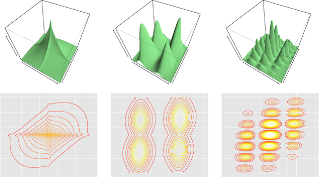
Figure 3: Densities of three 2-dimensional nonparanormals. The left plots have component functions of the form $f_{\alpha}(x)=\allowbreak\operatorname{sign}(x)|x|^{\alpha}$, with $\alpha_{1}=0.9$ and $\alpha_{2}=0.8$. The center plots have component functions of the form $g_{\alpha}(x)=\allowbreak\lfloor x\rfloor+1/(1+\exp(-\alpha(x-\lfloor x\rfloor-1/2)))$ with $\alpha_{1}=10$ and $\alpha_{2}=5$, where $x-\lfloor x\rfloor$ is the fractional part. The right plots have component functions of the form $h_{\alpha}(x)=x+\sin(\alpha x)/\alpha$, with $\alpha_{1}=5$ and $\alpha_{2}=10$. In each case $\mu=(0,0)$ and $\Sigma=\bigl{(}{{1\enskip 0.5}\atop{0.5\enskip 1}}\bigr{)}$.

In fact, this is true for any choice of identification restrictions; thus it is not necessary to estimate $\mu$ or $\sigma$ to estimate the graph, as the following result shows.

Lemma 3.1

Define

$$h_{j}(x)=\Phi^{-1}(F_{j}(x)),$$ (6)

and let $\Lambda$ be the covariance matrix of $h(X)$. Then $X_{j}\amalg X_{k}|X_{\backslash\{j,k\}}$ if and only if $\Lambda_{jk}^{-1}=0$.

We can rewrite the covariance matrix as

$$\Sigma_{jk}=\operatorname{Cov}(Z_{j},Z_{k})=\sigma_{j}\sigma_{k}\operatorname{Cov}(h_{j}(X_{j}),h_{k}(X_{k})).$$

Hence $\Sigma=D\Lambda D$ and

$$\Sigma^{-1}=D^{-1}\Lambda^{-1}D^{-1},$$

where $D$ is the diagonal matrix with $\operatorname{diag}(D)=\sigma$. The zero pattern of $\Lambda^{-1}$ is therefore identical to the zero pattern of $\Sigma^{-1}$.

Figure 3 shows three examples of 2-dimensional nonparanormal densities. The component functions are taken to be from three different families of monotonic functions—one using power transforms, one using logistic transforms and another using sinusoids.

$$f_{\alpha}(x) = \operatorname{sign}(x)|x|^{\alpha},$$

$$g_{\alpha}(x) = \lfloor x\rfloor+\frac{1}{1+\exp\{-\alpha(x-\lfloor x\rfloor-1/2)\}},$$

$$h_{\alpha}(x) = x+\frac{\sin(\alpha x)}{\alpha}.$$

The covariance in each case is $\Sigma=\bigl{(}{{1\enskip 0.5}\atop{0.5\enskip 1}}\bigr{)}$, and the mean is $\mu=(0,0)$. It can be seen how the concavity and number of modes of the density can change with different nonlinearities. Clearly the nonparanormal family is much richer than the Normal family.

The assumption that $f(X)=(f_{1}(X_{1}),\ldots,f_{d}(X_{d}))$ is Normal leads to a semiparametric model where only one-dimensional functions need to be estimated. But the monotonicity of the functions $f_{j}$, which map onto ${\mathbb{R}}$, enables computational tractability of the nonparanormal. For more general functions $f$, the normalizing constant for the density

$$p_{X}(x)\propto\exp\biggl{\{}-\frac{1}{2}\bigl{(}f(x)-\mu\bigr{)}^{T}{\Sigma}^{-1}\bigl{(}f(x)-\mu\bigr{)}\biggr{\}}$$

cannot be computed in closed form.

3.1 Connection to Copulæ

If $F_{j}$ is the distribution of $X_{j}$, then $U_{j}=F_{j}(X_{j})$ is uniformly distributed on $(0,1)$. Let $C$ denote the joint distribution function of $U=(U_{1},\ldots,U_{d})$, and let $F$ denote the distribution function of $X$. Then we have that

$$F(x_{1},\ldots,x_{d})$$

(7)

$$\quad={\mathbb{P}}(X_{1}\leq x_{1},\ldots,X_{d}\leq x_{d})$$

$$\quad={\mathbb{P}}\bigl{(}F_{1}(X_{1})$$

(8)

$$\hphantom{={\mathbb{P}}\bigl{(}}\quad\leq F_{1}(x_{1}),\ldots,F_{d}(X_{d})\leq F_{d}(x_{d})\bigr{)}$$

$$\quad={\mathbb{P}}\bigl{(}U_{1}\leq F_{1}(x_{1}),\ldots,U_{d}\leq F_{d}(x_{d})\bigr{)}$$ (9)

$$\quad=C(F_{1}(x_{1}),\ldots,F_{d}(x_{d})).$$ (10)

This is known as Sklar’s theorem ((Sklar, 1959)), and $C$ is called a copula. If $c$ is the density function of $C$, then

$$p(x_{1},\ldots,x_{d})$$

(11)

$$\quad=c(F_{1}(x_{1}),\ldots,F_{d}(x_{d}))\prod_{j=1}^{d}p(x_{j}),$$

where $p(x_{j})$ is the marginal density of $X_{j}$. For the nonparanormal we have

$$\quad F(x_{1},\ldots,x_{d})$$

(12)

$$\qquad=\Phi_{\mu,\Sigma}(\Phi^{-1}(F_{1}(x_{1})),\ldots,\Phi^{-1}(F_{d}(x_{d}))),$$

where $\Phi_{\mu,\Sigma}$ is the multivariate Gaussian cdf, and $\Phi$ is the univariate standard Gaussian cdf.

The Gaussian copula is usually expressed in terms of the correlation matrix, which is given by $R=\operatorname{diag}(\sigma)^{-1}\Sigma\operatorname{diag}(\sigma)^{-1}$. Note that the univariate mar ginal density for a Normal can be written as $p(x_{j})=\frac{1}{\sigma_{j}}\phi(u_{j})$ where $u_{j}=(x_{j}-\mu_{j})/\sigma_{j}$. The multivariate Normal density can thus be expressed as

$$p_{\mu,\Sigma}(x_{1},\ldots,x_{d})$$

$$\quad=\frac{1}{(2\pi)^{d/2}|R|^{1/2}\prod_{j=1}^{d}\sigma_{j}}$$ (13)

$$\qquad{}\cdot\exp\biggl{(}-\frac{1}{2}u^{T}R^{-1}u\biggr{)}$$

$$\quad=\frac{1}{|R|^{1/2}}\exp\biggl{(}-\frac{1}{2}u^{T}(R^{-1}-I)u\biggr{)}$$

(14)

$$\qquad{}\cdot\prod_{j=1}^{d}\frac{\phi(u_{j})}{\sigma_{j}}.$$

Since the distribution $F_{j}$ of the $j$th variable satisfies $F_{j}(x_{j})=\Phi((x_{j}-\mu_{j})/\sigma_{j})=\Phi(u_{j})$, we have that $(X_{j}-\mu_{j})/\sigma_{j}\stackrel{{\scriptstyle d}}{{=}}\Phi^{-1}(F_{j}(X_{j}))$. The Gaussian copula density is thus

$$c(F_{1}(x_{1}),\ldots,F_{d}(x_{d}))$$

$$\quad=\frac{1}{|R|^{1/2}}\exp\biggl{\{}-\frac{1}{2}\Phi^{-1}(F(x))^{T}$$ (15)

$$\qquad\hphantom{\frac{1}{|R|^{1/2}}\exp\biggl{\{}}{}\cdot(R^{-1}-I)\Phi^{-1}(F(x))\biggr{\}},$$

where

$$\Phi^{-1}(F(x))=(\Phi^{-1}(F_{1}(x_{1})),\ldots,\Phi^{-1}(F_{d}(x_{d}))).$$

This is seen to be equivalent to (3) using the chain rule and the identity

$$(\Phi^{-1})^{\prime}(\eta)=\frac{1}{\phi(\Phi^{-1}(\eta))}.$$ (16)

3.2 Estimation

Let $X^{(1)},\ldots,X^{(n)}$ be a sample of size $n$ where $X^{(i)}=(X^{(i)}_{1},\ldots,X^{(i)}_{d})^{T}\in\mathbb{R}^{d}$. We’ll design a two-step estimation procedure where first the functions $f_{j}$ are estimated, and then the inverse covariance matrix $\Omega$ is estimated, after transforming to approximately Normal.

In light of (6) we define

$$\widehat{h}_{j}(x)=\Phi^{-1}(\widetilde{F}_{j}(x)),$$

where $\widetilde{F}_{j}$ is an estimator of $F_{j}$. A natural candidate for $\widetilde{F}_{j}$ is the marginal empirical distribution function

$$\widehat{F}_{j}(t)\equiv\frac{1}{n}\sum_{i=1}^{n}\mathbf{1}_{\{X^{(i)}_{j}\leq t\}}.$$

However, in this case $\widehat{h}_{j}(x)$ blows up at the largest and smallest values of $X_{j}^{(i)}$. For the high-dimensional setting where $n$ is small relative to $d$, an attractive alternative is to use a truncated or Winsorized estimator,

$$\hskip 8.0pt\qquad\widetilde{F}_{j}(x)=\cases{\delta_{n},&\mbox{if $\widehat{F}_{j}(x)<\delta_{n}$,}\cr\widehat{F}_{j}(x),&\mbox{if $\delta_{n}\leq\widehat{F}_{j}(x)\leq 1-\delta_{n}$,}\cr(1-\delta_{n}),&\mbox{if $\widehat{F}_{j}(x)>1-\delta_{n}$},}$$ (17)

where $\delta_{n}$ is a truncation parameter. There is a bias–variance tradeoff in choosing $\delta_{n}$; increasing $\delta_{n}$ increases the bias while it decreases the variance.

Given this estimate of the distribution of variable $X_{j}$, we then estimate the transformation function $f_{j}$ by

$$\widetilde{f}_{j}(x)\equiv\widehat{\mu}_{j}+\widehat{\sigma}_{j}\widetilde{h}_{j}(x),$$ (18)

where

$$\widetilde{h}_{j}(x)=\Phi^{-1}(\widetilde{F}_{j}(x))$$

and $\widehat{\mu}_{j}$ and $\widehat{\sigma}_{j}$ are the sample mean and standard deviation.

$$\widehat{\mu}_{j}\equiv\frac{1}{n}\sum_{i=1}^{n}X^{(i)}_{j}\quad\mbox{and}\quad\widehat{\sigma}_{j}=\sqrt{\frac{1}{n}\sum_{i=1}^{n}\bigl{(}X^{(i)}_{j}-\widehat{\mu}_{j}\bigr{)}^{2}}.$$

Now, let $S_{n}(\widetilde{f})$ be the sample covariance matrix of $\widetilde{f}(X^{(1)}),\ldots,\widetilde{f}(X^{(n)})$; that is,

$$S_{n}(\widetilde{f}) \equiv \frac{1}{n}\sum_{i=1}^{n}\bigl{(}\widetilde{f}\bigl{(}X^{(i)}\bigr{)}-\mu_{n}(\widetilde{f})\bigr{)}$$

$$\hphantom{\frac{1}{n}\sum_{i=1}^{n}}{}\cdot\bigl{(}\widetilde{f}\bigl{(}X^{(i)}\bigr{)}-\mu_{n}(\widetilde{f})\bigr{)}^{T},$$

$$\mu_{n}(\widetilde{f}) \equiv \frac{1}{n}\sum_{i=1}^{n}\widetilde{f}\bigl{(}X^{(i)}\bigr{)}.$$

We then estimate $\Omega$ using $S_{n}(\widetilde{f})$. For instance, the maximum likelihood estimator is $\widehat{\Omega}^{\mathrm{MLE}}_{n}=S_{n}(\widetilde{f})^{-1}$.

The $\ell_{1}$-regularized estimator is

$$\widehat{\Omega}_{n} = \operatorname{arg\,min}\limits_{\Omega}\{\operatorname{tr}(\Omega S_{n}(\widetilde{f}))$$

$$\hphantom{\operatorname{arg\,min}\limits_{\Omega}\{}{}-\log|\Omega|+\lambda\|\Omega\|_{1}\},$$

where $\lambda$ is a regularization parameter, and $\|\Omega\|_{1}=\sum_{j=1}^{d}\sum_{k=1}^{d}|\Omega_{jk}|$. The estimated graph is then $\widehat{E}_{n}=\{(j,k)\dvtx\widehat{\Omega}_{jk}\neq 0\}$.

Thus we use a two-step procedure to estimate the graph:

Replace the observations, for each variable, by their respective Normal scores, subject to a Winsorized truncation.

Apply the graphical lasso to the transformed data to estimate the undirected graph.

The first step is noniterative and computationally efficient. The truncation parameter $\delta_{n}$ is chosen to be

$$\delta_{n}=\frac{1}{4n^{1/4}\sqrt{\pi\log n}}$$ (21)

and does not need to be tuned. As will be shown in Theorem 3.1, such a choice makes the nonparanormal amenable to theoretical analysis.

3.3 Statistical Properties of $S_{n}(\widetilde{f})$

The main technical result is an analysis of the covariance of the Winsorized estimator above. In particular, we show that under appropriate conditions,

$$\max_{j,k}|S_{n}(\widetilde{f})_{jk}-S_{n}(f)_{jk}|=O_{P}\Biggl{(}\sqrt{\frac{\log d+\log^{2}n}{n^{1/2}}}\Biggr{)},$$

where $S_{n}(\widetilde{f})_{jk}$ denotes the $(j,k)$ entry of the matrix $S_{n}(\widetilde{f})$. This result allows us to leverage the significant body of theory on the graphical lasso ((Rothman et al., 2008); (Ravikumar et al., 2009)) which we apply in step two.

Theorem 3.1

Suppose that $d=n^{\xi}$, and let $\widetilde{f}$ be the Winsorized estimator defined in (18) with $\delta_{n}=\frac{1}{4n^{1/4}\sqrt{\pi\log n}}$. Define

$$C(M,\xi)\equiv\frac{48}{\sqrt{\pi\xi}}\bigl{(}\sqrt{2M}-1\bigr{)}(M+2)$$

for $M,\xi>0$. Then for any $\varepsilon\geq C(M,\xi)\sqrt{\frac{\log d+\log^{2}n}{n^{1/2}}}$ and sufficiently large $n$, we have

$$\mathbb{P}\Bigl{(}\max_{jk}|S_{n}(\widetilde{f})_{jk}-S_{n}(f)_{jk}|>\varepsilon\Bigr{)}$$

$$\quad\leq\frac{c_{1}d}{(n\varepsilon^{2})^{2\xi}}+\frac{c_{2}d}{n^{M\xi-1}}+c_{3}\exp\biggl{(}-\frac{c_{4}n^{1/2}\varepsilon^{2}}{\log d+\log^{2}n}\biggr{)},$$

where $c_{1},c_{2},c_{3},c_{4}$ are positive constants.

The proof of this result involves a detailed Gaussian tail analysis, and is given in Liu, Lafferty and Wasserman (2009).

Using Theorem 3.1 and the results of Rothman et al. (2008), it can then be shown that the precision matrix is estimated at the following rates in the Frobenius norm and the $\ell_{2}$-operator norm:

$$\|\widehat{\Omega}_{n}-\Omega_{0}\|_{\mathrm{F}}=O_{P}\biggl{(}\sqrt{\frac{(s+d)\log d+\log^{2}n}{n^{1/2}}}\biggr{)}$$

and

$$\|\widehat{\Omega}_{n}-\Omega_{0}\|_{2}=O_{P}\biggl{(}\sqrt{\frac{s\log d+\log^{2}n}{n^{1/2}}}\biggr{)},$$

where

$$s\equiv\operatorname{Card}\bigl{(}\{(i,j) \in \{1,\ldots,d\}\{1,\ldots,d\}|$$

$$\hskip 8.0pt{}\Omega_{0}(i,j)\neq 0,i\neq j\}\bigr{)}$$

is the number of nonzero off-diagonal elements of the true precision matrix.

Using the results of Ravikumar et al. (2009), it can also be shown, under appropriate conditions, that the sparsity pattern of the precision matrix is estimated accurately with high probability. In particular, the nonparanormal estimator $\widehat{\Omega}_{n}$ satisfies

$$\mathbb{P}(\mathcal{G}(\widehat{\Omega}_{n},\Omega_{0}))\geq 1-o(1),$$

where $\mathcal{G}(\widehat{\Omega}_{n},\Omega_{0})$ is the event

$$\bigl{\{}\operatorname{sign}(\widehat{\Omega}_{n}(j,k))=\operatorname{sign}(\Omega_{0}(j,k)),\forall j,k\in\{1,\ldots,d\}\bigr{\}}.$$

We refer to Liu, Lafferty and Wasserman (2009) for the details of the conditions and proofs. These $\widetilde{O}_{P}(n^{-1/4})$ rates are slower than the $\widetilde{O}_{P}(n^{-1/2})$ rates obtainable for the graphical lasso. However, in more recent work ((Liu et al., 2012)) we use estimators based on Spearman’s rho and Kendall’s tau statistics to obtain the parametric rate.

4 Forest Density Estimation

We now describe a very different, but equally flexible and useful approach. Rather than assuming a transformation to normality and an arbitrary undirected graph, we restrict the graph to be a tree or forest, but allow arbitrary nonparametric distributions.

Let $p^{*}(x)$ be a probability density with respect to Lebesgue measure $\mu(\cdot)$ on $\mathbb{R}^{d}$, and let $X^{(1)},\ldots,X^{(n)}$ be $n$ independent identically distributed $\mathbb{R}^{d}$-valued data vectors sampled from $p^{*}(x)$ where $X^{(i)}=(X^{(i)}_{1},\break\ldots,X^{(i)}_{d})$. Let $\mathcal{X}_{j}$ denote the range of $X_{j}^{(i)}$, and let $\mathcal{X}=\mathcal{X}_{1}\times\cdots\times\mathcal{X}_{d}$.

A graph is a forest if it is acyclic. If $F$ is a $d$-node undirected forest with vertex set $V_{F}=\{1,\ldots,d\}$ and edge set $E_{F}\subset\{1,\ldots,d\}\times\{1,\ldots,d\}$, the number of edges satisfies $|E_{F}|<d$. We say that a probability density function $p(x)$ is supported by a forest $F$ if the density can be written as

$$p_{F}(x)=\prod_{(i,j)\in E_{F}}\frac{p(x_{i},x_{j})}{p(x_{i})p(x_{j})}\prod_{k\in V_{F}}p(x_{k}),$$ (22)

where each $p(x_{i},x_{j})$ is a bivariate density on $\mathcal{X}_{i}\times X_{j}$, and each $p(x_{k})$ is a univariate density on $\mathcal{X}_{k}$.

Let $\mathcal{F}_{d}$ be the family of forests with $d$ nodes, and let $\mathcal{P}_{d}$ be the corresponding family of densities.

$$\qquad\mathcal{P}_{d} = \biggl{\{}p\geq 0\dvtx\int_{\mathcal{X}}p(x)\,d\mu(x)=1,\mbox{ and}$$

$$\hphantom{\{}{}\mbox{$p(x)$ satisfies (\ref{eq.treedensity}) for some $F\in\mathcal{F}_{d}$}\biggr{\}}.$$

Define the oracle forest density

$$q^{*}=\operatorname{arg\,min}\limits_{q\in\mathcal{P}_{d}}D(p^{*}\|q)$$ (24)

where the Kullback–Leibler divergence $D(p\|q)$ between two densities $p$ and $q$ is

$$D(p\|q)=\int_{\mathcal{X}}p(x)\log\frac{p(x)}{q(x)}\,dx,$$ (25)

under the convention that $0\log(0/q)=0$, and$p\log(p/0)=\infty$ for $p\neq 0$. The following is straightforward to prove.

Proposition 4.1

Let $q^{*}$ be defined as in (24). There exists a forest $F^{*}\in\mathcal{F}_{d}$, such that

$$q^{*} = p^{*}_{F^{*}}$$

$$= \prod_{(i,j)\in E_{F^{*}}}\frac{p^{*}(x_{i},x_{j})}{p^{*}(x_{i})p^{*}(x_{j})}\prod_{k\in V_{F^{*}}}p^{*}(x_{k}),$$

where $p^{*}(x_{i},x_{j})$ and $p^{*}(x_{i})$ are the bivariate and univariate marginal densities of $p^{*}$.

For any density $q(x)$, the negative log-likelihood risk $R(q)$ is defined as

$$R(q) = -\mathbb{E}\log q(X)$$

$$= -\int_{\mathcal{X}}p^{*}(x)\log q(x)\,dx.$$

It is straightforward to see that the density $q^{*}$ defined in (24) also minimizes the negative log-likelihood loss.

$$q^{*} = \operatorname{arg\,min}\limits_{q\in\mathcal{P}_{d}}D(p^{*}\|q)$$

$$= \operatorname{arg\,min}\limits_{q\in\mathcal{P}_{d}}R(q).$$

We thus define the oracle risk as $R^{*}=R(q^{*})$. Using Proposition 4.1 and equation (22), we have

$$R^{*} = R(q^{*})=R(p^{*}_{F^{*}})$$

$$= -\int_{\mathcal{X}}p^{*}(x)\biggl{(}\sum_{(i,j)\in E_{F^{*}}}\log\frac{p^{*}(x_{i},x_{j})}{p^{*}(x_{i})p^{*}(x_{j})}$$

$$\hskip 83.0pt{}+\sum_{k\in V_{F^{*}}}\log(p^{*}(x_{k}))\biggr{)}\,dx$$

$$= -\sum_{(i,j)\in E_{F^{*}}}I(X_{i};X_{j})+\sum_{k\in V_{F^{*}}}H(X_{k}),$$

where

$$\quad I(X_{i};X_{j}) = \int_{\mathcal{X}_{i}\times\mathcal{X}_{j}}p^{*}(x_{i},x_{j})$$

$$\hphantom{\int_{\mathcal{X}_{i}\times\mathcal{X}_{j}}}{}\cdot\log\frac{p^{*}(x_{i},x_{j})}{p^{*}(x_{i})p^{*}(x_{j})}\,dx_{i}\,dx_{j}$$

is the mutual information between the pair of variables $X_{i}$, $X_{j}$, and

$$H(X_{k})=-\int_{\mathcal{X}_{k}}p^{*}(x_{k})\log p^{*}(x_{k})\,dx_{k}$$ (31)

is the entropy.

4.1 A Two-Step Procedure

If the true density $p^{*}(x)$ were known, by Proposition 4.1, the density estimation problem would be reduced to finding the best forest structure $F^{*}_{d}$, satisfying

$$F^{*}_{d} = \operatorname{arg\,min}\limits_{F\in\mathcal{F}_{d}}R(p^{*}_{F})$$

$$= \operatorname{arg\,min}\limits_{F\in\mathcal{F}_{d}}D(p^{*}\|p^{*}_{F}).$$

The optimal forest $F^{*}_{d}$ can be found by minimizing the right-hand side of (4). Since the entropy term $H(X)=\sum_{k}H(X_{k})$ is constant across all forests, this can be recast as the problem of finding the maximum weight spanning forest for a weighted graph, where the weight of the edge connecting nodes $i$ and $j$ is $I(X_{i};X_{j})$. Kruskal’s algorithm ((Kruskal, 1956)) is a greedy algorithm that is guaranteed to find a maximum weight spanning tree of a weighted graph. In the setting of density estimation, this procedure was proposed by Chow and Liu (1968) as a way of constructing a tree approximation to a distribution. At each stage the algorithm adds an edge connecting that pair of variables with maximum mutual information among all pairs not yet visited by the algorithm, if doing so does not form a cycle. When stopped early, after $k<d-1$ edges have been added, it yields the best $k$-edge weighted forest.

Of course, the above procedure is not practical since the true density $p^{*}(x)$ is unknown. We replace the population mutual information $I(X_{i};X_{j})$ in (4) by a plug-in estimate $\widehat{I}_{n}(X_{i};X_{j})$, defined as

$$\widehat{I}_{n}(X_{i};X_{j}) = \int_{\mathcal{X}_{i}\times\mathcal{X}_{j}}\widehat{p}_{n}(x_{i},x_{j})$$

$$\hphantom{\int_{\mathcal{X}_{i}\times\mathcal{X}_{j}}}{}\cdot\log\frac{\widehat{p}_{n}(x_{i},x_{j})}{\widehat{p}_{n}(x_{i})\widehat{p}_{n}(x_{j})}\,dx_{i}\,dx_{j},$$

where $\widehat{p}_{n}(x_{i},x_{j})$ and $\widehat{p}_{n}(x_{i})$ are bivariate and univariate kernel density estimates. Given this estimated mutual information matrix $\widehat{M}_{n}=[\widehat{I}_{n}(X_{i};X_{j})]$, we can then apply Kruskal’s algorithm (equivalently, the Chow–Liu algorithm) to find the best tree structure $\widehat{F}_{n}$.

Since the number of edges of $\widehat{F}_{n}$ controls the number of degrees of freedom in the final density estimator, an automatic data-dependent way to choose it is needed. We adopt the following two-stage procedure. First, we randomly split the data into two sets $\mathcal{D}_{1}$ and $\mathcal{D}_{2}$ of sizes $n_{1}$ and $n_{2}$; we then apply the following steps:

Using $\mathcal{D}_{1}$, construct kernel density estimates of the univariate and bivariate marginals and calculate $\widehat{I}_{n_{1}}(X_{i};X_{j})$ for $i,j\in\{1,\ldots,d\}$ with $i\neq j$. Construct a full tree $\widehat{F}^{(d-1)}_{n_{1}}$ with $d-1$ edges, using the Chow–Liu algorithm.

Using $\mathcal{D}_{2}$, prune the tree $\widehat{F}^{(d-1)}_{n_{1}}$ to find a forest $\widehat{F}^{(\widehat{k})}_{n_{1}}$ with $\widehat{k}$ edges, for $0\leq\widehat{k}\leq d-1$.

Once $\widehat{F}^{(\widehat{k})}_{n_{1}}$ is obtained in Step 2, we can calculate $\widehat{p}_{\widehat{F}^{(\widehat{k})}_{n_{1}}}$ according to (22), using the kernel density estimates constructed in Step 1.

4.1.1 Step 1: Constructing a sequence of forests

Step 1 is carried out on the dataset $\mathcal{D}_{1}$. Let $K(\cdot)$ be a univariate kernel function. Given an evaluation point $(x_{i},x_{j})$, the bivariate kernel density estimate for $(X_{i},X_{j})$ based on the observations $\{X^{(s)}_{i},\break X^{(s)}_{j}\}_{s\in\mathcal{D}_{1}}$ is defined as

$$\qquad\widehat{p}_{n_{1}}(x_{i},x_{j})$$

(34)

$$\quad\qquad=\frac{1}{n_{1}}\sum_{s\in\mathcal{D}_{1}}\frac{1}{h^{2}_{2}}K\biggl{(}\frac{X^{(s)}_{i}-x_{i}}{h_{2}}\biggr{)}K\biggl{(}\frac{X^{(s)}_{j}-x_{j}}{h_{2}}\biggr{)},$$

where we use a product kernel with $h_{2}>0$ as the bandwidth parameter. The univariate kernel density estimate $\widehat{p}_{n_{1}}(x_{k})$ for $X_{k}$ is

$$\widehat{p}_{n_{1}}(x_{k})=\frac{1}{n_{1}}\sum_{s\in\mathcal{D}_{1}}\frac{1}{h_{1}}K\biggl{(}\frac{X^{(s)}_{k}-x_{k}}{h_{1}}\biggr{)},$$ (35)

where $h_{1}>0$ is the univariate bandwidth.

We assume that the data lie in a $d$-dimensional unit cube $\mathcal{X}=[0,1]^{d}$. To calculate the empirical mutual information $\widehat{I}_{n_{1}}(X_{i};X_{j})$, we need to numerically evaluate a two-dimensional integral. To do so, we calculate the kernel density estimates on a grid of points. We choose $m$ evaluation points on each dimension, $x_{1i}<x_{2i}<\cdots<x_{mi}$ for the $i$th variable. The mutual information $\widehat{I}_{n_{1}}(X_{i};X_{j})$ is then approximated as

$$\widehat{I}_{n_{1}}(X_{i};X_{j})$$

$$\quad=\frac{1}{m^{2}}\sum_{k=1}^{m}\sum_{\ell=1}^{m}\widehat{p}_{n_{1}}(x_{ki},x_{\ell j})$$ (36)

$$\qquad\hphantom{\frac{1}{m^{2}}\sum_{k=1}^{m}\sum_{\ell=1}^{m}}{}\cdot\log\frac{\widehat{p}_{n_{1}}(x_{ki},x_{\ell j})}{\widehat{p}_{n_{1}}(x_{ki})\widehat{p}_{n_{1}}(x_{\ell j})}.$$

The approximation error can be made arbitrarily small by choosing $m$ sufficiently large. As a practical concern, care needs to be taken that the factors $\widehat{p}_{n_{1}}(x_{ki})$ and $\widehat{p}_{n_{1}}(x_{\ell j})$ in the denominator are not too small; a truncation procedure can be used to ensure this. Once the $d\times d$ mutual information matrix $\widehat{M}_{n_{1}}=[\widehat{I}_{n_{1}}(X_{i};X_{j})]$ is obtained, we can apply the Chow–Liu (Kruskal) algorithm to find a maximum weight spanning tree (see Algorithm 1).

Algorithm 1 Tree construction (Kruskal/Chow–Liu)

Input: Data set $\mathcal{D}_{1}$ and the bandwidths $h_{1}$, $h_{2}$.

Initialize: Calculate $\widehat{M}_{n_{1}}$, according to (4.1.1), (35) and (4.1.1).

Set $E^{(0)}=\varnothing$.

For $k=1,\ldots,d-1$:

 (1) Set $(i^{(k)},j^{(k)})\leftarrow\operatorname{arg\,max}_{(i,j)}\widehat{M}_{n_{1}}(i,j)$ such that $E^{(k-1)}\cup\{(i^{(k)},j^{(k)})\}$ does not contain a cycle;

 (2) $E^{(k)}\leftarrow E^{(k-1)}\cup\{(i^{(k)},j^{(k)})\}$.

Output: tree $\widehat{F}^{(d-1)}_{n_{1}}$ with edge set $E^{(d-1)}$.

4.1.2 Step 2: Selecting a forest size

The full tree $\widehat{F}^{(d-1)}_{n_{1}}$ obtained in Step 1 might have high variance when the dimension $d$ is large, leading to overfitting in the density estimate. In order to reduce the variance, we prune the tree; that is, we choose an unconnected tree with $k$ edges. The number of edges $k$ is a tuning parameter that induces a bias–variance tradeoff.

In order to choose $k$, note that in stage $k$ of the Chow–Liu algorithm, we have an edge set $E^{(k)}$ (in the notation of the Algorithm 1) which corresponds to a forest $\widehat{F}^{(k)}_{n_{1}}$ with $k$ edges, where $F^{(0)}_{n_{1}}$ is the union of $d$ disconnected nodes. To select $k$, we cross-validate over the $d$ forests $\widehat{F}^{(0)}_{n_{1}},\widehat{F}^{(1)}_{n_{1}},\ldots,\widehat{F}^{(d-1)}_{n_{1}}$.

Let $\widehat{p}_{n_{2}}(x_{i},x_{j})$ and $\widehat{p}_{n_{2}}(x_{k})$ be defined as in (4.1.1) and (35), but now evaluated solely based on the held-out data in $\mathcal{D}_{2}$. For a density $p_{F}$ that is supported by a forest $F$, we define the held-out negative log-likelihood risk as

$$\widehat{R}_{n_{2}}(p_{F})$$

$$\quad=-\sum_{(i,j)\in E_{F}}\int_{\mathcal{X}_{i}\times\mathcal{X}_{j}}\widehat{p}_{n_{2}}(x_{i},x_{j})$$

$$\qquad\hphantom{-\sum_{(i,j)\in E_{F}}\int_{\mathcal{X}_{i}\times\mathcal{X}_{j}}}{}\cdot\log\frac{p(x_{i},x_{j})}{p(x_{i})p(x_{j})}\,dx_{i}\,dx_{j}$$

$$\qquad-\sum_{k\in V_{F}}\int_{\mathcal{X}_{k}}\widehat{p}_{n_{2}}(x_{k})\log p(x_{k})\,dx_{k}.$$

The selected forest is then $\widehat{F}^{(\widehat{k})}_{n_{1}}$ where

$$\widehat{k}=\operatorname{arg\,min}\limits_{k\in\{0,\ldots,d-1\}}\widehat{R}_{n_{2}}(\widehat{p}_{F^{(k)}_{n_{1}}})$$ (38)

and where $\widehat{p}_{F^{(k)}_{n_{1}}}$ is computed using the density estimate $\widehat{p}_{n_{1}}$ constructed on $\mathcal{D}_{1}$.

We can also estimate $\widehat{k}$ as

$$\quad\widehat{k} = \operatorname{arg\,max}\limits_{k\in\{0,\ldots,d-1\}}\frac{1}{n_{2}}$$

$${}\cdot\sum_{s\in\mathcal{D}_{2}}\log\biggl{(}\prod_{(i,j)\in E_{F^{(k)}}}\frac{\widehat{p}_{n_{1}}(X^{(s)}_{i},X^{(s)}_{j})}{\widehat{p}_{n_{1}}(X^{(s)}_{i})\widehat{p}_{n_{1}}(X^{(s)}_{j})}$$

$$\hskip 103.0pt{}\cdot\prod_{\ell\in V_{F^{(k)}}}\widehat{p}_{n_{1}}\bigl{(}X^{(s)}_{\ell}\bigr{)}\biggr{)}$$

$$= \operatorname{arg\,max}\limits_{k\in\{0,\ldots,d-1\}}\frac{1}{n_{2}}$$

$${}\cdot\sum_{s\in\mathcal{D}_{2}}\log\biggl{(}\prod_{(i,j)\in E_{F^{(k)}}}\frac{\widehat{p}_{n_{1}}(X^{(s)}_{i},X^{(s)}_{j})}{\widehat{p}_{n_{1}}(X^{(s)}_{i})\widehat{p}_{n_{1}}(X^{(s)}_{j})}\biggr{)}.$$

This minimization can be efficiently carried out by iterating over the $d-1$ edges in $\widehat{F}^{(d-1)}_{n_{1}}$.

Once $\widehat{k}$ is obtained, the final forest-based kernel density estimate is given by

$$\qquad\widehat{p}_{n}(x)=\prod_{(i,j)\in E^{(\widehat{k})}}\frac{\widehat{p}_{n_{1}}(x_{i},x_{j})}{\widehat{p}_{n_{1}}(x_{i})\widehat{p}_{n_{1}}(x_{j})}\prod_{k}\widehat{p}_{n_{1}}(x_{k}).$$ (41)

Another alternative is to compute a maximum weight spanning forest, using Kruskal’s algorithm, but with held-out edge weights

$$\hskip 20.0pt\widehat{w}_{n_{2}}(i,j)=\frac{1}{n_{2}}\sum_{s\in\mathcal{D}_{2}}\log\frac{\widehat{p}_{n_{1}}(X^{(s)}_{i},X^{(s)}_{j})}{\widehat{p}_{n_{1}}(X^{(s)}_{i})\widehat{p}_{n_{1}}(X^{(s)}_{j})}.$$ (42)

In fact, asymptotically (as $n_{2}\rightarrow\infty$) this gives an optimal tree-based estimator constructed in terms of the kernel density estimates $\widehat{p}_{n_{1}}$.

4.2 Statistical Properties

The statistical properties of the forest density estimator can be analyzed under the same type of assumptions that are made for classical kernel density estimation. In particular, assume that the univariate and bivariate densities lie in a Hölder class with exponent $\beta$. Under this assumption the minimax rate of convergence in the squared error loss is $O(n^{\beta/(\beta+1)})$ for bivariate densities and $O(n^{2\beta/(2\beta+1)})$ for univariate densities. Technical assumptions on the kernel yield $L_{\infty}$ concentration results on kernel density estimation ((Giné and Guillou, 2002)).

Choose the bandwidths $h_{1}$ and $h_{2}$ to be used in the one-dimensional and two-dimensional kernel density estimates according to

$$h_{1} \asymp \biggl{(}\frac{\log n}{n}\biggr{)}^{1/(1+2\beta)},$$ (43)

$$h_{2} \asymp \biggl{(}\frac{\log n}{n}\biggr{)}^{1/(2+2\beta)}.$$ (44)

This choice of bandwidths ensures the optimal rate of convergence. Let $\mathcal{P}^{(k)}_{d}$ be the family of $d$-dimensional densities that are supported by forests with at most $k$ edges. Then

$$\mathcal{P}^{(0)}_{d}\subset\mathcal{P}^{(1)}_{d}\subset\cdots\subset\mathcal{P}^{(d-1)}_{d}.$$ (45)

Due to this nesting property,

$$\inf_{q_{F}\in\mathcal{P}^{(0)}_{d}}R(q_{F}) \geq \inf_{q_{F}\in\mathcal{P}^{(1)}_{d}}R(q_{F})$$

$$\geq \cdots\geq\inf_{q_{F}\in\mathcal{P}^{(d-1)}_{d}}R(q_{F}).$$

This means that a full spanning tree would generally be selected if we had access to the true distribution. However, with access to finite data to estimate the densities ($\widehat{p}_{n_{1}}$), the optimal procedure is to use fewer than $d-1$ edges. The following result analyzes the excess risk resulting from selecting the forest based on the heldout risk $\widehat{R}_{n_{2}}$.

Theorem 4.1

Let $\widehat{p}_{\widehat{F}^{(k)}_{d}}$ be the estimate with $|E_{\widehat{F}^{(k)}_{d}}|=k$ obtained after the first $k$ iterations of the Chow–Liu algorithm. Then under (omitted) technical assumptions on the densities and kernel, for any $1\leq k\leq d-1$,

$$\quad R(\widehat{p}_{\widehat{F}^{(k)}_{d}})-\inf_{q_{F}\in\mathcal{P}^{(k)}_{d}}R(q_{F})$$

(47)

$$\qquad=O_{P}\biggl{(}k\sqrt{\frac{\log n+\log d}{n^{\beta/(1+\beta)}}}+d\sqrt{\frac{\log n+\log d}{n^{2\beta/(1+2\beta)}}}\biggr{)}$$

and

$$R(\widehat{p}_{\widehat{F}^{(\widehat{k})}_{d}})-\min_{0\leq k\leq d-1}R(\widehat{p}_{\widehat{F}^{(k)}_{d}})$$

$$\quad=O_{P}\Biggl{(}(k^{*}+\widehat{k})\sqrt{\frac{\log n+\log d}{n^{\beta/(1+\beta)}}}$$ (48)

$$\hskip 43.0pt\qquad{}+d\sqrt{\frac{\log n+\log d}{n^{2\beta/(1+2\beta)}}}\Biggr{)},$$

where $\widehat{k}=\operatorname{arg\,min}_{0\leq k\leq d-1}\widehat{R}_{n_{2}}(\widehat{p}_{\widehat{F}^{(k)}_{d}})$ and $k^{*}=\break\operatorname{arg\,min}_{0\leq k\leq d-1}R(\widehat{p}_{\widehat{F}^{(k)}_{d}})$.

The main work in proving this result lies in establishing bounds such as

$$\sup_{F\in\mathcal{F}^{(k)}_{d}}|R(\widehat{p}_{F})-\widehat{R}_{n_{2}}(\widehat{p}_{F})|$$

(49)

$$\quad=O_{P}\bigl{(}\phi_{n}(k)+\psi_{n}(d)\bigr{)},$$

where $\widehat{R}_{n_{2}}$ is the held-out risk, under the notation

$$\phi_{n}(k) = k\sqrt{\frac{\log n+\log d}{n^{\beta/(\beta+1)}}},$$ (50)

$$\psi_{n}(d) = d\sqrt{\frac{\log n+\log d}{n^{2\beta/(1+2\beta)}}}.$$ (51)

For the proof of this and related results, see Liu et al. (2011). Using this, one easily obtains

$$R(\widehat{p}_{\widehat{F}^{(\widehat{k})}_{d}})-R(\widehat{p}_{\widehat{F}^{(k^{*})}_{d}})$$

$$\quad=R(\widehat{p}_{\widehat{F}^{(\widehat{k})}_{d}})-\widehat{R}_{n_{2}}(\widehat{p}_{\widehat{F}^{(\widehat{k})}_{d}})$$ (52)

$$\qquad{}+\widehat{R}_{n_{2}}(\widehat{p}_{\widehat{F}^{(\widehat{k})}_{d}})-R(\widehat{p}_{\widehat{F}^{(k^{*})}_{d}})$$

$$\quad=O_{P}\bigl{(}\phi_{n}(\widehat{k})+\psi_{n}(d)\bigr{)}$$

(53)

$$\qquad{}+\widehat{R}_{n_{2}}(\widehat{p}_{\widehat{F}^{(\widehat{k})}_{d}})-R(\widehat{p}_{\widehat{F}^{(k^{*})}_{d}})$$

$$\quad\leq O_{P}\bigl{(}\phi_{n}(\widehat{k})+\psi_{n}(d)\bigr{)}$$

(54)

$$\qquad{}+\widehat{R}_{n_{2}}(\widehat{p}_{\widehat{F}^{(k^{*})}_{d}})-R(\widehat{p}_{\widehat{F}^{(k^{*})}_{d}})$$

$$\quad=O_{P}\bigl{(}\phi_{n}(\widehat{k})+\phi_{n}(k^{*})+\psi_{n}(d)\bigr{)},$$ (55)

where (4.2) follows from the fact that $\widehat{k}$ is the minimizer of $\widehat{R}_{n_{2}}(\cdot)$. This result allows the dimension $d$ to increase at a rate $o(\sqrt{n^{2\beta/(1+2\beta)}/\log n})$, and the number of edges $k$ to increase at a rate $o(\sqrt{n^{\beta/(1+\beta)}/\log n})$, with the excess risk still decreasing to zero asymptotically.

Note that the minimax rate for 2-dimensional kernel density estimation under our stated conditions is $n^{-\beta/(\beta+1)}$. The rate above is essentially the square root of this rate, up to logarithmic factors. This is because a higher order kernel is used, which may result in negative values. Once we correct these negative values, the resulting estimated density will no longer integrate to one. The slower rate is due to a very simple truncation technique to correct the higher-order kernel density estimator to estimate mutual information. Current work is investigating a different version of the higher order kernel density estimator with more careful correction techniques, for which it is possible to achieve the optimal minimax rate.

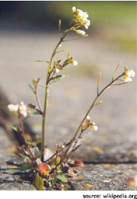
Figure 4: Arabidopsis thaliana is a small flowering plant; it was the first plant genome to be sequenced, and its roughly 27,000 genes and 35,000 proteins have been actively studied. Here we consider a data set based on Affymetrix GeneChip microarrays with sample size $n=118$, for which $d=40$ genes have been selected for analysis.

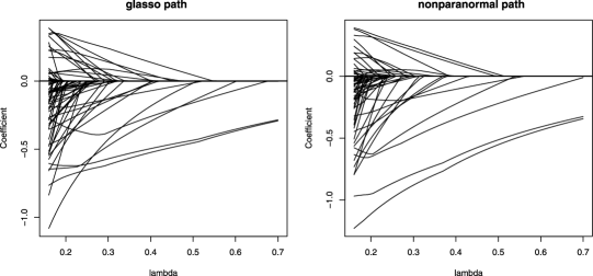
Figure 5: Regularization paths of both methods on the microarray data set. Although the paths for the two methods look similar, there are some subtle differences.

In theory the bandwidths are chosen as in (43) and (44), assuming $\beta$ is known. In our experiments presented below, the bandwidth $h_{k}$ for the 2-dimensional kernel density estimator is chosen according to the Normal reference rule

$$h_{k} = 1.06\cdot\min\biggl{\{}\widehat{\sigma}_{k},\frac{\widehat{q}_{k,0.75}-\widehat{q}_{k,0.25}}{1.34}\biggr{\}}$$

$${}\cdot n^{-1/(2\beta+2)},$$

where $\widehat{\sigma}_{k}$ is the sample standard deviation of $\{X^{(s)}_{k}\}_{s\in\mathcal{D}_{1}}$, and $\widehat{q}_{k,0.75}$, $\widehat{q}_{k,0.25}$ are the $75\%$ and $25\%$ sample quantiles of $\{X^{(s)}_{k}\}_{s\in\mathcal{D}_{1}}$, with $\beta=2$. See Wasserman (2006) for a discussion of this choice of bandwidth.

5 Examples

5.1 Gene–Gene Interaction Graphs

The nonparanormal and Gaussian graphical model can construct very different graphs. Here we consider a data set based on Affymetrix GeneChip microarrays for the plant Arabidopsis thaliana (Wille et al., 2004) (see Figure 4). The sample size is $n=118$. The expression levels for each chip are pre-processed by log-transformation and standardization. A subset of 40 genes from the isoprenoid pathway is chosen for analysis.

While these data are often treated as multivariate Gaussian, the nonparanormal and the glasso give very different graphs over a wide range of regularization parameters, suggesting that the nonparametric method could lead to different biological conclusions.

The regularization paths of the two methods are compared in Figure 5. To generate the paths, we select 50 regularization parameters on an evenly spaced grid in the interval $[0.16,1.2]$. Although the paths for the two methods look similar, there are some subtle differences. In particular, variables become nonzero in a different order.

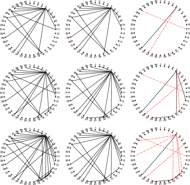
Figure 6: The nonparanormal estimated graph for three values of $\lambda=0.2448,0.2661,0.30857$ (left column), the closest glasso estimated graph from the full path (middle) and the symmetric difference graph (right).

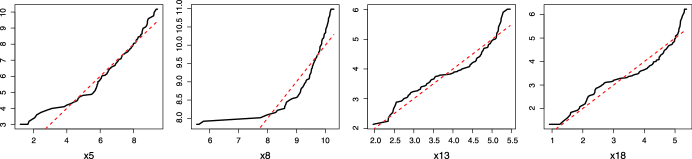
Figure 7: Estimated transformation functions for four genes in the microarray data set, indicating non-Gaussian marginals. The corresponding genes are among the nodes appearing in the symmetric difference graphs above.

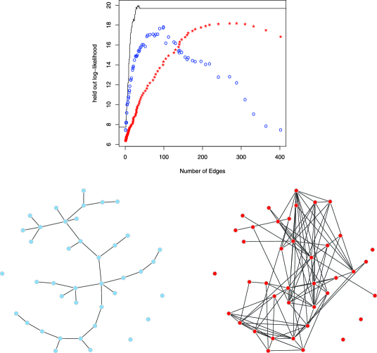
Figure 8: Results on microarray data. Top: held-out log-likelihood of the forest density estimator (black step function), glasso (red stars) and refit glasso (blue circles). Bottom: estimated graphs using the forest-based estimator (left) and the glasso (right), using the same node layout.

Figure 6 compares the estimated graphs for the two methods at several values of the regularization parameter $\lambda$ in the range $[0.16,0.37]$. For each $\lambda$, we show the estimated graph from the nonparanormal in the first column. In the second column we show the graph obtained by scanning the full regularization path of the glasso fit and finding the graph having the smallest symmetric difference with the nonparanormal graph. The symmetric difference graph is shown in the third column. The closest glasso fit is different, with edges selected by the glasso not selected by the nonparanormal, and vice-versa. The estimated transformation functions for several genes are shown Figure 7, which show non-Gaussian behavior.

Since the graphical lasso typically results in a large parameter bias as a consequence of the $\ell_{1}$ regularization, it sometimes make sense to use the refit glasso, which is a two-step procedure—in the first step, a sparse inverse covariance matrix is obtained by the graphical lasso; in the second step, a Gaussian model is refit without $\ell_{1}$ regularization, but enforcing the sparsity pattern obtained in the first step.

Figure 8 compares forest density estimation to the graphical lasso and refit glasso. It can be seen that the forest-based kernel density estimator has better generalization performance. This is not surprising, given that the true distribution of the data is not Gaussian. (Note that since we do not directly compute the marginal univariate densities in the nonparanormal, we are unable to compute likelihoods under this model.) The held-out log-likelihood curve for forest density estimation achieves a maximum when there are only 35 edges in the model. In contrast, the held-out log-likelihood curves of the glasso and refit glasso achieve maxima when there are around 280 edges and 100 edges respectively, while their predictive estimates are still inferior to those of the forest-based kernel density estimator. Figure 8 also shows the estimated graphs for the forest-based kernel density estimator and the graphical lasso. The graphs are automatically selected based on held-out log-likelihood, and are clearly different.

Target Corp. (Consumer Discr.) Big Lots, Inc. (Consumer Discr.) Costco Co. (Consumer Staples) Family Dollar Stores (Consumer Discr.) Kohl’s Corp. (Consumer Discr.) Lowe’s Cos. (Consumer Discr.) Macy’s Inc. (Consumer Discr.) Wal-Mart Stores (Consumer Staples)

Yahoo Inc. (Information Tech.) Amazon.com Inc. (Consumer Discr.) eBay Inc. (Information Tech.) NetApp (Information Tech.)

Figure 9: Example neighborhoods in a forest graph for two stocks, Yahoo Inc. and Target Corp. The corresponding GICS industries are shown in parentheses. (Consumer Discr. is short for Consumer Discretionary, and Information Tech. is short for Information Technology.)

5.2 Graphs for Equities Data

For the examples in this section we collected stock price data from Yahoo! Finance (finance.yahoo.com). The daily closing prices were obtained for 452 stocks that consistently were in the S&P 500 index between January 1, 2003 through January 1, 2011. This gave us altogether 2015 data points, each data point corresponds to the vector of closing prices on a trading day. With $S_{t,j}$ denoting the closing price of stock $j$ on day $t$, we consider the variables $X_{tj}=\log(S_{t,j}/S_{t-1,j})$ and build graphs over the indices $j$. We simply treat the instances $X_{t}$ as independent replicates, even though they form a time series. The data contain many outliers; the reasons for these outliers include splits in a stock, which increases the number of shares. We Winsorize (or truncate) every stock so that its data points are within three times the mean absolute deviation from the sample average. The importance of this Winsorization is shown below; see the “snake graph” in Figure 10. For the following results we use the subset of the data between January 1, 2003 to January 1, 2008, before the onset of the “financial crisis.” It is interesting to compare to results that include data after 2008, but we omit these for brevity.

The 452 stocks are categorized into 10 Global Industry Classification Standard (GICS) sectors, including Consumer Discretionary (70 stocks),Consumer Staples (35 stocks), Energy (37 stocks), Financials (74 stocks), Health Care (46 stocks), Industrials (59 stocks), Information Tech-nology (64 stocks), Materials (29 stocks), Telecommunications Services (6 stocks), and Utilities (32 stocks). In the graphs shown below, the nodes are colored according to the GICS sector of the corresponding stock. It is expected that stocks from the same GICS sectors should tend to be clustered together, since stocks from the same GICS sector tend to interact more with each other. This is indeed this case; for example, Figure 9 shows examples of the neighbors of two stocks, Yahoo Inc. and Target Corp., in the forest density graph.

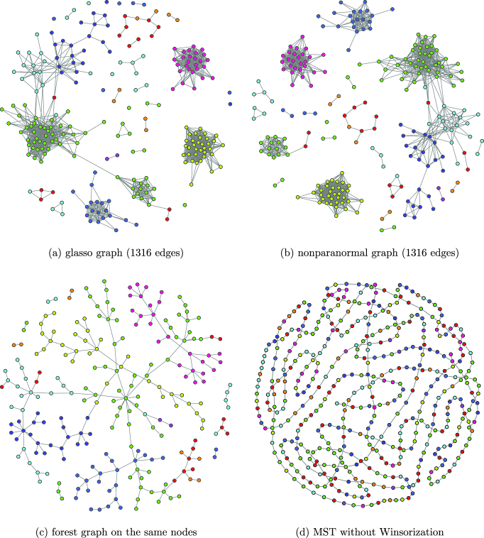
Figure 10: Graphs build on S&P 500 stock data from Jan. 1, 2003 to Jan. 1, 2008. The graphs are estimated using (a) the glasso, (b) the nonparanormal and (c) forest density estimation. The nodes are colored according to their GICS sector categories. Nodes are not shown that have zero neighbors in both the glasso and nonparanormal graphs. Figure (d) shows the maximum weight spanning tree that results if the data are not Winsorized to trim outliers.

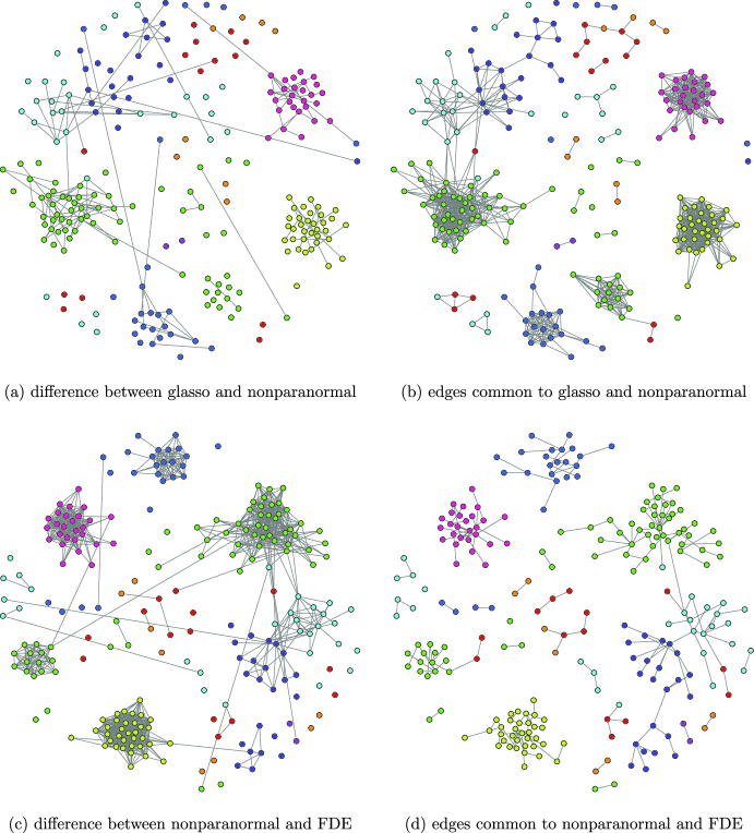
Figure 11: Visualizations of the differences and similarities between the estimated graphs. The symmetric difference between the glasso and nonparanormal graphs is shown in (a), and the edges common to the graphs are shown in (b). Similarly, the symmetric difference between the nonparanormal and forest density estimate is shown in (c), and the common edges are shown in (d).

Figures 10(a)–(c) show graphs estimated using the glasso, nonparanormal, and forest density estimator on the data from January 1, 2003 to January 1, 2008. There are altogether $n=1257$ data points and $d=452$ dimensions. To estimate the glasso graph, we somewhat arbitrarily set the regularization parameter to $\lambda=0.55$, which results in a graph that has 1316 edges, about 3 neighbors per node, and good clustering structure. The resulting graph is shown in Figure 10(a). The corresponding nonparanormal graph is shown in Figure 10(b). The regularization is chosen so that it too has 1316 edges. Only nodes that have neighbors in one of the graphs are shown; the remaining nodes are disconnected.

Since our dataset contains $n=1257$ data points, we directly apply the forest density estimator on the whole dataset to obtain a full spanning tree of $d-1=451$ edges. This estimator turns out to be very sensitive to outliers, since it exploits kernel density estimates as building blocks. In Figure 10(d) we show the estimated forest density graph on the stock data when outliers are not trimmed by Winsorization. In this case the graph is anomolous, with a snake-like character that weaves in and out of the 10 GICS industries. Intuitively, the outliers make the two-dimensional densities appear like thin “pancakes,” and densities with similar orientations are clustered together. To address this, we trim the outliers by Winsorizing at 3 MADs, as described above. Figure 10(c) shows the estimated forest graph, restricted to the same stocks shown for the graphs in (a) and (b). The resulting graph has good clustering with respect to the GICS sectors.

Figures 11(a)–(c) display the differences and edges common to the glasso, nonparanormal and forest graphs. Figure 11(a) shows the symmetric difference between the estimated glasso and nonparanormal graphs, and Figure 11(b) shows the common edges. Figure 11(c) shows the symmetric difference between the nonparanormal and forest graphs, and Figure 11(d) shows the common edges.

We refrain from drawing any hard conclusionsabout the effectiveness of the different methods based on these plots—how these graphs are used will depend on the application. These results serve mainly to highlight how very different inferences about the independence relations can arise from moving from a Gaussian model to a semiparametric model to a fully nonparametric model with restricted graphs.

6 Related Work

There is surprisingly little work on structure learning of nonparametric graphical models in high dimensions. One piece of related work is sparse log-density smoothing spline ANOVA models, introduced by Jeon and Lin (2006). In such a model the log-density function is decomposed as the sum of a constant term, one-dimensional functions (main effects), two-dimensional functions (two-way interactions) and so on.

$$\hskip 18.0pt\log p(x) = f(x)$$

$$\equiv c+\sum_{j=1}^{d}f_{j}(x_{j})+\sum_{j<k}f_{jk}(x_{j},x_{k})+\cdots.$$

The component functions satisfy certain constraints so that the model is identifiable. In high dimensions, the model is truncated up to second order interactions so that the computation is still tractable. There is a close connection between the log-density ANOVA model and undirected graphical models. For a model with only main effects and two-way interactions, we define a graph $G=(V,E)$ such that $(i,j)\in E$ if and only if $f_{ij}\neq 0$. It can be seen that $p(x)$ is Markov to $G$. Jeon and Lin (2006) assume that these component functions belong to certain reproducing kernel Hilbert spaces (RKHSs) equipped with a RKHS norm $\|\cdot\|_{K}$. To obtain a sparse estimation of the component functions $f(x)$, they propose a penalized M-estimator,

$$\widehat{f} = \operatorname{arg\,max}\limits_{f}\Biggl{\{}\frac{1}{n}\sum_{i=1}^{n}\exp\bigl{(}f\bigl{(}X^{(i)}\bigr{)}\bigr{)}$$

$$\hskip 40.0pt{}+\int f(x)\rho(x)\,dx+\lambda J(f)\Biggr{\}},$$

where $\rho(x)$ is some pre-defined positive density, and $J(f)$ is a sparsity-inducing penalty that takes the form

$$J(f)=\sum_{j=1}^{d}\|f_{j}\|_{K}+\sum_{j<k}\|f_{jk}\|_{K}.$$ (59)

Solving (6) only requires one-dimensional integrals which can be efficiently computed. However, the optimization in (6) exploits a surrogate loss instead of the log-likelihood loss, and is more difficult to analyze theoretically.

Another related idea is to conduct structure learning using nonparametric decomposable graphicalmodels ((Schwaighofer et al., 2007)). A distribution is a decomposable graphical model if it is Markov to a graph $G=(V,E)$ which has a junction tree representation, which can be viewed as an extension of tree-based graphical models. A junction tree yields a factorized form

$$p(x)=\frac{\prod_{C\in V_{T}}p(x_{C})}{\prod_{S\in E_{T}}p(x_{S})},$$ (60)

where $V_{T}$ denotes the set of cliques in $V$, and $E_{T}$ is the set of separators, that is, the intersection of two neighboring cliques in the junction tree. Exact search for the junction tree structure that maximizes the likelihood is usually computationally expensive. Schwaighofer et al. (2007) propose a forward–backward strategy for nonparametric structure learning. However, such a greedy procedure does not guarantee that the global optimal solution is found, and makes theoretical analysis challenging.

7 Discussion

This paper has considered undirected graphical models for continuous data, where the general densities take the form

$$p(x)\propto\exp\biggl{(}\sum_{C\in\mathrm{Cliques}(G)}f_{C}(x_{C})\biggr{)}.$$ (61)

Such a general family is at least as difficult as the general high-dimensional nonparametric regression model. But, as for regression, simplifying assumptions can lead to tractable and useful models. We have considered two approaches that make very different tradeoffs between statistical generality and computational efficiency. The nonparanormal relies on estimating one-dimensional functions, in a manner that is similar to the way additive models estimate one-dimensional regression functions. This allows arbitrary graphs, but the distribution is semiparametric, via the Gaussian copula. At the other extreme, when we restrict to acyclic graphs we can have fully nonparametric bivariate and univariate marginals. This leverages classical techniques for low-dimensional density estimation, together with approximation algorithms for constructing the graph. Clearly these are just two among many possibilities for nonparametric graphical modeling. We conclude, then, with a brief description of a few potential directions for future work.

As we saw with the nonparanormal, if only the graph is of interest, it may not be important to estimate the functions accurately. More generally, to estimate the graph it is not necessary to estimate the density. One of the most effective and theoretically well-supported methods for estimating Gaussian graphs is due to Meinshausen and Bühlmann (2006). In this approach, we regress each variable $X_{j}$ onto all other variables $(X_{k})_{k\neq j}$ using the lasso. This directly estimates the set of neighbors ${\mathcal{N}}(j)=\{k|(j,k)\in E\}$ for each node $j$ in the graph, but the covariance matrix is not directly estimated. Lasso theory gives conditions and guarantees on these variable selection problems. This approach was adapted to the discrete case by Ravikumar, Wainwright and Lafferty (2010), where the normalizing constant and thus the density can’t be efficiently computed. This general strategy may be attractive for graph selection in nonparametric graphical models. In particular, each variable could be regressed on the others using a nonparametric regression method that performs variable selection; one such method with theoretical guarantees is due to Lafferty and Wasserman (2008).

A different framework for nonparametricity involves conditioning on a collection of observed explanatory variables $Z$. Liu et al. (2010) develop a nonparametric procedure called Graph-optimized CART, or Go-CART, to estimate the graph conditionally under a Gaussian model. The main idea is to build a tree partition on the $Z$ space just as in CART (classification and regression trees), but to estimate a graph at each leaf using the glasso. Oracle inequalities on risk minimization and model selection consistency were established for Go-CART by Liu et al. (2010). When $Z$ is time, graph-valued regression reduces to the time-varying graph estimation problem ((Chen et al., 2010); (Kolar et al., 2010); Zhou, Lafferty and Wasserman, 2010).

Another fruitful direction is the introduction of latent variables. Even though the graphical model of the observed variables $X$ may be complex, when conditioned on some latent explanatory variables $Z$, the graph may be simplified. One straightforward approach is to build mixtures of the models we consider here. A mixture of nonparanormals will require new methods, to compute the derivatives $f^{\prime}_{j}(x_{j})$. A mixture of forests could be implemented using a kind of nonparametric EM algorithm, with kernel density estimates over weighted data in the M-step. But it is not easy to read off a graph from a mixture model.

In parametric settings, Chandrasekaran, Parrilo and Willsky (2010) and Choi et al. (2010) develop algorithms and theory for learning graphical models with latent variables. The first paper assumes the joint distribution of the observed and latent variables is a Gaussian graphical model, and the second paper assumes the joint distribution is discrete and factors according to a forest. Since the nonparanormal and forest density estimator are nonparametric versions of the Gaussian and forest graphical models for discrete data, we expect similar techniques to those of Chandrasekaran, Parrilo and Willsky (2010), Choi et al. (2010) can be used to extend our methods to handle latent variables. It would also be of interest to formulate nonparametric extensions of low rank plus sparse covariance matrices.

No matter how the methodology develops, nonparametric graphical models will at best be approximations to the true distribution in many applications. Yet, there is plenty of experience to show how incorrect models can be useful. An ongoing challenge in nonparametric graphical modeling will be to better understand how the structure can be accurately estimated even when the model is wrong.

References

- Banerjee, El Ghaoui and d’Aspremont (2008) {barticle}[mr] \bauthor\bsnmBanerjee, \bfnmOnureena\binitsO., \bauthor\bsnmEl Ghaoui, \bfnmLaurent\binitsL. and \bauthor\bsnmd’Aspremont, \bfnmAlexandre\binitsA. (\byear2008). \btitleModel selection through sparse maximum likelihood estimation for multivariate Gaussian or binary data. \bjournalJ. Mach. Learn. Res. \bvolume9 \bpages485–516. \bidissn=1532-4435, mr=2417243 \bptokimsref \endbibitem
- Chandrasekaran, Parrilo and Willsky (2010) {bmisc}[auto:STB—2012/06/07—11:40:19] \bauthor\bsnmChandrasekaran, \bfnmV.\binitsV., \bauthor\bsnmParrilo, \bfnmP. A.\binitsP. A. and \bauthor\bsnmWillsky, \bfnmA. S.\binitsA. S. (\byear2010). \bhowpublishedLatent variable graphical model selection via convex optimization. Available at http://arxiv.org/abs/ 1008.1290. \bptokimsref \endbibitem
- Chen et al. (2010) {bincollection}[auto:STB—2012/06/07—11:40:19] \bauthor\bsnmChen, \bfnmX.\binitsX., \bauthor\bsnmLiu, \bfnmY.\binitsY., \bauthor\bsnmLiu, \bfnmH.\binitsH. and \bauthor\bsnmCarbonell, \bfnmJ. G.\binitsJ. G. (\byear2010). \btitleLearning spatial–temporal varying graphs with applications to climate data analysis. In \bbooktitleAAAI-10: Twenty-Fourth Conference on Artificial Intelligence (AAAI) \bpublisherAAAI Press, \baddressMenlo Park, CA. \bptokimsref \endbibitem
- Choi et al. (2010) {bmisc}[mr] \bauthor\bsnmChoi, \bfnmM. J.\binitsM. J., \bauthor\bsnmTan, \bfnmV. Y.\binitsV. Y., \bauthor\bsnmAnandkumar, \bfnmA.\binitsA. and \bauthor\bsnmWillsky, \bfnmA. S.\binitsA. S. (\byear2010). \bhowpublishedLearning latent tree graphical models. Available at http://arxiv.org/abs/1009.2722. \bptokimsref \endbibitem
- Chow and Liu (1968) {barticle}[auto:STB—2012/06/07—11:40:19] \bauthor\bsnmChow, \bfnmC.\binitsC. and \bauthor\bsnmLiu, \bfnmC.\binitsC. (\byear1968). \btitleApproximating discrete probability distributions with dependence trees. \bjournalIEEE Transactions on Information Theory \bvolume14 \bpages462–467. \bptokimsref \endbibitem
- Friedman, Hastie and Tibshirani (2007) {barticle}[auto:STB—2012/06/07—11:40:19] \bauthor\bsnmFriedman, \bfnmJ. H.\binitsJ. H., \bauthor\bsnmHastie, \bfnmT.\binitsT. and \bauthor\bsnmTibshirani, \bfnmR.\binitsR. (\byear2007). \btitleSparse inverse covariance estimation with the graphical lasso. \bjournalBiostatistics \bvolume9 \bpages432–441. \bptokimsref \endbibitem
- Giné and Guillou (2002) {barticle}[mr] \bauthor\bsnmGiné, \bfnmEvarist\binitsE. and \bauthor\bsnmGuillou, \bfnmArmelle\binitsA. (\byear2002). \btitleRates of strong uniform consistency for multivariate kernel density estimators. \bjournalAnn. Inst. H. Poincaré Probab. Stat. \bvolume38 \bpages907–921. \biddoi=10.1016/S0246-0203(02)01128-7, issn=0246-0203, mr=1955344 \bptokimsref \endbibitem
- Jeon and Lin (2006) {barticle}[mr] \bauthor\bsnmJeon, \bfnmYongho\binitsY. and \bauthor\bsnmLin, \bfnmYi\binitsY. (\byear2006). \btitleAn effective method for high-dimensional log-density ANOVA estimation, with application to nonparametric graphical model building. \bjournalStatist. Sinica \bvolume16 \bpages353–374. \bidissn=1017-0405, mr=2267239 \bptokimsref \endbibitem
- Kolar et al. (2010) {barticle}[mr] \bauthor\bsnmKolar, \bfnmMladen\binitsM., \bauthor\bsnmSong, \bfnmLe\binitsL., \bauthor\bsnmAhmed, \bfnmAmr\binitsA. and \bauthor\bsnmXing, \bfnmEric P.\binitsE. P. (\byear2010). \btitleEstimating time-varying networks. \bjournalAnn. Appl. Stat. \bvolume4 \bpages94–123. \biddoi=10.1214/09-AOAS308, issn=1932-6157, mr=2758086 \bptnotecheck year\bptokimsref \endbibitem
- Kruskal (1956) {barticle}[mr] \bauthor\bsnmKruskal, \bfnmJoseph B.\binitsJ. B. \bsuffixJr. (\byear1956). \btitleOn the shortest spanning subtree of a graph and the traveling salesman problem. \bjournalProc. Amer. Math. Soc. \bvolume7 \bpages48–50. \bidissn=0002-9939, mr=0078686 \bptokimsref \endbibitem
- Lafferty and Wasserman (2008) {barticle}[mr] \bauthor\bsnmLafferty, \bfnmJohn\binitsJ. and \bauthor\bsnmWasserman, \bfnmLarry\binitsL. (\byear2008). \btitleRodeo: Sparse, greedy nonparametric regression. \bjournalAnn. Statist. \bvolume36 \bpages28–63. \biddoi=10.1214/009053607000000811, issn=0090-5364, mr=2387963 \bptokimsref \endbibitem
- Liu, Lafferty and Wasserman (2009) {barticle}[mr] \bauthor\bsnmLiu, \bfnmHan\binitsH., \bauthor\bsnmLafferty, \bfnmJohn\binitsJ. and \bauthor\bsnmWasserman, \bfnmLarry\binitsL. (\byear2009). \btitleThe nonparanormal: Semiparametric estimation of high dimensional undirected graphs. \bjournalJ. Mach. Learn. Res. \bvolume10 \bpages2295–2328. \bidissn=1532-4435, mr=2563983 \bptokimsref \endbibitem
- Liu et al. (2010) {bincollection}[auto:STB—2012/06/07—11:40:19] \bauthor\bsnmLiu, \bfnmH.\binitsH., \bauthor\bsnmChen, \bfnmX.\binitsX., \bauthor\bsnmLafferty, \bfnmJ.\binitsJ. and \bauthor\bsnmWasserman, \bfnmL.\binitsL. (\byear2010). \btitleGraph-valued regression. In \bbooktitleProceedings of the Twenty-Third Annual Conference on Neural Information Processing Systems (NIPS). \bptokimsref \endbibitem
- Liu et al. (2011) {barticle}[mr] \bauthor\bsnmLiu, \bfnmHan\binitsH., \bauthor\bsnmXu, \bfnmMin\binitsM., \bauthor\bsnmGu, \bfnmHaijie\binitsH., \bauthor\bsnmGupta, \bfnmAnupam\binitsA., \bauthor\bsnmLafferty, \bfnmJohn\binitsJ. and \bauthor\bsnmWasserman, \bfnmLarry\binitsL. (\byear2011). \btitleForest density estimation. \bjournalJ. Mach. Learn. Res. \bvolume12 \bpages907–951. \biddoi=10.1016/j.micres.2009.11.010, issn=1532-4435, mr=2786914 \bptokimsref \endbibitem
- Liu et al. (2012) {binproceedings}[author] \bauthor\bsnmLiu, \bfnmHan\binitsH., \bauthor\bsnmHan, \bfnmFang\binitsF., \bauthor\bsnmYuan, \bfnmMing\binitsM., \bauthor\bsnmLafferty, \bfnmJohn\binitsJ. and \bauthor\bsnmWasserman, \bfnmLarry\binitsL. (\byear2012). \btitleHigh dimensional semiparametric Gaussian copula graphical models. In \bbooktitleProceedings of the 29th International Conference on Machine Learning (ICML-12). \bpublisherACM, \baddressNew York. \bptokimsref \endbibitem
- Mallows (1990) {bbook}[mr] \beditor\bsnmMallows, \bfnmColin L.\binitsC. L., ed. (\byear1990). \btitleThe Collected Works of John W. Tukey. Vol. VI: More Mathematical: 1938–1984. \bpublisherWadsworth & Brooks/Cole Advanced Books & Software, \baddressPacific Grove, CA. \bidmr=1057793 \bptnotecheck related\bptokimsref \endbibitem
- Meinshausen and Bühlmann (2006) {barticle}[mr] \bauthor\bsnmMeinshausen, \bfnmNicolai\binitsN. and \bauthor\bsnmBühlmann, \bfnmPeter\binitsP. (\byear2006). \btitleHigh-dimensional graphs and variable selection with the lasso. \bjournalAnn. Statist. \bvolume34 \bpages1436–1462. \biddoi=10.1214/009053606000000281, issn=0090-5364, mr=2278363 \bptokimsref \endbibitem
- Ravikumar, Wainwright and Lafferty (2010) {barticle}[mr] \bauthor\bsnmRavikumar, \bfnmPradeep\binitsP., \bauthor\bsnmWainwright, \bfnmMartin J.\binitsM. J. and \bauthor\bsnmLafferty, \bfnmJohn D.\binitsJ. D. (\byear2010). \btitleHigh-dimensional Ising model selection using -regularized logistic regression. \bjournalAnn. Statist. \bvolume38 \bpages1287–1319. \biddoi=10.1214/09-AOS691, issn=0090-5364, mr=2662343 \bptokimsref \endbibitem
- Ravikumar et al. (2009) {bincollection}[auto:STB—2012/06/07—11:40:19] \bauthor\bsnmRavikumar, \bfnmP.\binitsP., \bauthor\bsnmWainwright, \bfnmM.\binitsM., \bauthor\bsnmRaskutti, \bfnmG.\binitsG. and \bauthor\bsnmYu, \bfnmB.\binitsB. (\byear2009). \btitleModel selection in Gaussian graphical models: High-dimensional consistency of -regularized MLE. In \bbooktitleAdvances in Neural Information Processing Systems, \bvolume22 \bpublisherMIT Press, \baddressCambridge, MA. \bptokimsref \endbibitem
- Rothman et al. (2008) {barticle}[mr] \bauthor\bsnmRothman, \bfnmAdam J.\binitsA. J., \bauthor\bsnmBickel, \bfnmPeter J.\binitsP. J., \bauthor\bsnmLevina, \bfnmElizaveta\binitsE. and \bauthor\bsnmZhu, \bfnmJi\binitsJ. (\byear2008). \btitleSparse permutation invariant covariance estimation. \bjournalElectron. J. Stat. \bvolume2 \bpages494–515. \biddoi=10.1214/08-EJS176, issn=1935-7524, mr=2417391 \bptokimsref \endbibitem
- Schwaighofer et al. (2007) {bincollection}[auto:STB—2012/06/07—11:40:19] \bauthor\bsnmSchwaighofer, \bfnmA.\binitsA., \bauthor\bsnmDejori, \bfnmM.\binitsM., \bauthor\bsnmTresp, \bfnmV.\binitsV. and \bauthor\bsnmStetter, \bfnmM.\binitsM. (\byear2007). \btitleStructure learning with nonparametric decomposable models. In \bbooktitleProceedings of the 17th International Conference on Artificial Neural Networks. ICANN’07. \bpublisherElsevier, \baddressNew York. \bptokimsref \endbibitem
- Sklar (1959) {barticle}[mr] \bauthor\bsnmSklar, \bfnmM.\binitsM. (\byear1959). \btitleFonctions de répartition à dimensions et leurs marges. \bjournalPubl. Inst. Statist. Univ. Paris \bvolume8 \bpages229–231. \bidmr=0125600 \bptokimsref \endbibitem
- Wasserman (2006) {bbook}[mr] \bauthor\bsnmWasserman, \bfnmLarry\binitsL. (\byear2006). \btitleAll of Nonparametric Statistics. \bpublisherSpringer, \baddressNew York. \bidmr=2172729 \bptokimsref \endbibitem
- Wille et al. (2004) {barticle}[auto:STB—2012/06/07—11:40:19] \bauthor\bsnmWille, \bfnmA.\binitsA., \bauthor\bsnmZimmermann, \bfnmP.\binitsP., \bauthor\bsnmVranová, \bfnmE.\binitsE., \bauthor\bsnmFürholz, \bfnmA.\binitsA., \bauthor\bsnmLaule, \bfnmO.\binitsO., \bauthor\bsnmBleuler, \bfnmS.\binitsS., \bauthor\bsnmHennig, \bfnmL.\binitsL., \bauthor\bsnmPrelić, \bfnmA.\binitsA., \bauthor\bparticlevon \bsnmRohr, \bfnmP.\binitsP., \bauthor\bsnmThiele, \bfnmL.\binitsL., \bauthor\bsnmZitzler, \bfnmE.\binitsE., \bauthor\bsnmGruissem, \bfnmW.\binitsW. and \bauthor\bsnmBühlmann, \bfnmP.\binitsP. (\byear2004). \btitleSparse Gaussian graphical modelling of the isoprenoid gene network in Arabidopsis thaliana. \bjournalGenome Biology \bvolume5 \bpagesR92. \bptokimsref \endbibitem
- Yuan and Lin (2007) {barticle}[mr] \bauthor\bsnmYuan, \bfnmMing\binitsM. and \bauthor\bsnmLin, \bfnmYi\binitsY. (\byear2007). \btitleModel selection and estimation in the Gaussian graphical model. \bjournalBiometrika \bvolume94 \bpages19–35. \biddoi=10.1093/biomet/asm018, issn=0006-3444, mr=2367824 \bptokimsref \endbibitem
- Zhou, Lafferty and Wasserman (2010) {barticle}[auto:STB—2012/06/07—11:40:19] \bauthor\bsnmZhou, \bfnmS.\binitsS., \bauthor\bsnmLafferty, \bfnmJ.\binitsJ. and \bauthor\bsnmWasserman, \bfnmL.\binitsL. (\byear2010). \btitleTime varying undirected graphs. \bjournalMach. Learn. \bvolume80 \bpages295–329. \bptokimsref \endbibitem