The Hunt for Exomoons with Kepler (HEK):
I. Description of a New Observational Project

Abstract

Two decades ago, empirical evidence concerning the existence and frequency of planets around stars, other than our own, was absent. Since this time, the detection of extrasolar planets from Jupiter-sized to most recently Earth-sized worlds has blossomed and we are finally able to shed light on the plurality of Earth-like, habitable planets in the cosmos. Extrasolar moons may also be frequent habitable worlds but their detection or even systematic pursuit remains lacking in the current literature. Here, we present a description of the first systematic search for extrasolar moons as part of a new observational project called “The Hunt for Exomoons with Kepler” (HEK). The HEK project distills the entire list of known transiting planet candidates found by Kepler (2326 at the time of writing) down to the most promising candidates for hosting a moon. Selected targets are fitted using a multimodal nested sampling algorithm coupled with a planet-with-moon light curve modelling routine. By comparing the Bayesian evidence of a planet-only model to that of a planet-with-moon, the detection process is handled in a Bayesian framework. In the case of null detections, upper limits derived from posteriors marginalised over the entire prior volume will be provided to inform the frequency of large moons around viable planetary hosts, $\eta_{\leftmoon}$. After discussing our methodologies for target selection, modelling, fitting and vetting, we provide two example analyses.

1. INTRODUCTION

Extrasolar moons represent an outstanding challenge in modern observational astronomy. Their detection and study would yield a revolution in the understanding of planet/moon formation and evolution, but perhaps most provocatively they could be frequent seats for life in the Galaxy (Williams et al., 1997). Their existence is widely speculated both from a Copernican perspective and simulations of planet synthesis (Elser et al., 2011), and yet their detection has remained elusive.

In truth, very little effort has been spent on the search for moons relative to their planetary counterparts, presumably due to the known difficulty such a feat represents. Indeed, there has never been a systematic search for exomoons and just a handful of papers have attempted to detect their presence in several transiting planet systems (Brown et al., 2001; Kipping & Bakos, 2011a, b) (Lewis 2011 provide a extensive discussion regarding non-transiting moons around pulsar planets). With Kepler now boasting 2326 candidate transiting planets (Batalha et al., 2012), we can consider this candidate list to be comparable to target list of stars used in radial velocity surveys, for example. Further, Kepler is specifically designed to detect Earth-sized transiting objects and thus has the capability to find large moons (Kipping et al., 2009). In light of this, the time is ripe for the first systematic program to search for the satellites of extrasolar planets and so in this paper we describe our new observational project: “The Hunt for Exomoons with Kepler” (HEK).

The objective of the HEK project is to inspect the most viable planetary candidates for evidence of an exomoon, using publicly available Kepler photometry. In cases of a null-detection, and when conditions permit, the obtained constraints will be used to inform a new statistic in exoplanetary science: the frequency of large moons, $\eta_{\leftmoon}$.

The structure of the paper is as follows. In §2, we will present an overview of the current literature regarding the existence of exomoons, which will inform our search. In a similar vein, §3 presents an overview of the current literature on the observational consequences of exomoons. In §4, the multi-pronged HEK target selection process will be described, which greatly aids in refining the search to only the most favourable objects. §5 discusses the detection, modelling and fitting strategy of the HEK project, with particular focus on the use of Bayesian evidence and the application of a multimodal nested sampling algorithm, MultiNest, in combination with our exomoon-modelling code, LUNA. In §6, we explore the process of vetting exomoon candidates against false-positives, such as perturbing planets. §7 presents two examples of the MultiNest algorithm with LUNA on synthetic data, illustrating the use of Bayesian evidence for detections. Finally, we summarise the project’s goals and methods in §8. A list of acronyms used throughout this work is available in the Appendix, Table LABEL:tab:acros. Similarly, a list of mathematical symbols and notation used in this work is found in Table LABEL:tab:parameters.

2. EXOMOONS

2.1. Definition

An extrasolar moon, or exomoon, is a natural satellite of a extrasolar planet. Our project will focus on the detection of satellites which are gravitationally bound to be within the Hill sphere of their host planet, as opposed to quasi-satellites which can reside outside.

For a planet with a single large moon, it is possible that a more appropriate description would be a binary-planet. The blurry line between a binary-planet and a true planet-moon pair can be drawn by the point at which the centre of mass of two bodies lies outside the radius of both bodies. This distinction is merely a taxonomical issue though and in principle the HEK project can also detect binary planets, should they exist.

2.2. Observational Effects of an Exomoon

A detailed discussion of how we will search for exomoons is presented in §3. However, for the purposes of providing some context in the subsequent sections, we will briefly outline the observational consequences of an exomoon. The HEK project will search for moons around transiting extrasolar planets and thus primarily make use of photometry (specifically photometry obtained by Kepler). For an overview of alternative exomoon detection techniques, see Kipping (2011b). For transiting planet systems, a companion moon can reveal itself through two categories of observational effects:

• Dynamical variations of the host planet.

• Eclipse features induced by the moon.

Dynamical effects are measured as perturbations of the motion of the host planet away from a simple Keplerian orbit. It is thought that the most observable dynamical effects will be transit timing and duration variations (TTV and TDV respectively) (Sartoretti & Schneider, 1999; Szabó et al., 2006; Kipping, 2009a, b). Dynamical effects primarily reveal information about the exomoon mass.

Eclipse features are caused by the moon either occulting the stellar light directly or inducing so-called “mutual events” (Ragozzine & Holman, 2010) by occulting the planet during a planet-star eclipse. In either case, such events primarily reveal information about the exomoon radius.

2.3. Feasibly Detectable Systems

Kipping et al. (2009) conducted a feasibility study of Kepler’s sensitivity to a habitable-zone gas giant with a single moon, based upon dynamical effects only (i.e. TTV & TDV). The study assumed moons were on coplanar, circular orbits around their host planet. They found that Kepler should be sensitive to exomoons of masses $\gtrsim 0.2$ $M_{\oplus}$, in the most favourable circumstances. Even in this optimistic case, this is an order-of-magnitude more massive than the most massive moon in our Solar System, specifically Ganymede at $0.025$ $M_{\oplus}$. Consequently, it must be understood that HEK is searching for moons in a mass regime which do not exist within our own Solar System. We dub these moons as “large moons” and place a definition of such a moon as being $\gtrsim 10^{-1}$ $M_{\oplus}$. Again, this is an arbitrary distinction but is useful for the HEK project.

We point out that HEK will be more sensitive than the limits in Kipping et al. (2009) due to the fact that we will also search for eclipses caused by the moon. This additional information means that we must be at least as sensitive as using dynamics alone, but should become significantly more sensitive by including this extra information. An in-depth analysis of our sensitivity to exomoons is beyond the scope of this work. We consider such an analysis unnecessary in light of the fact that each system studied will have upper limits derived and so the detectability of moons will become apparent as the project develops. At this time, we consider a far more useful application of our efforts to be in actually conducting the search.

2.4. Plausible Origin of Large Moons

Given that no large moons ($M_{S}\gtrsim 10^{-1}$ $M_{\oplus}$) exist in the Solar System, how likely is it that such an object exists? The first important point to make is that two classes of moons exist: regular satellites and irregular satellites. In discussing the plausibility of a large moon around a planet, there are two issues to consider: i) origin ii) evolution. In other words, the moon must have some initial plausible formation/origin scenario and second it must survive long enough to be detected. We here discuss the former issue.

Regular satellites are those which are believed to have formed in-situ around the host planet as it accumulates gas and rock-ice solids from solar orbit. Canup & Ward (2006) predict that the cumulative moon mass is constrained via $\sum M_{S,i}\lesssim 2\times 10^{-4}$ $M_{P}$, where $M_{P}$ is the mass of the planet host. This limit is caused by a balance of two competing processes; the supply of inflowing material to the satellites, and satellite loss through orbital decay driven by the gas. Thus, for Jupiter-like masses, large moons should not form. Although brown-dwarfs could harbour Earth-mass moons, the mass ratio remains too small for TTV/TDV methods to feasibly infer their presence. Therefore, we argue it is unlikely HEK will detect any regular satellites if the Canup & Ward (2006) scaling law holds.

Irregular satellites are those which are obtained from a non-local origin such as capture (e.g. Triton; Agnor & Hamilton 2006) or impact scenarios (e.g. the Moon; Taylor 1992). Such moons could reach large masses so long as they are dynamically stable. This means that Earth-mass moons (or even larger) are plausible and HEK would be sensitive to such objects. Unlike regular satellites, irregular moons may frequently reside in retrograde orbits too (Porter & Grundy, 2011).

In order for a planet to capture a large moon, an essentially terrestrial-mass object must be dynamically captured by a larger body. The probability of such an event occurring is a topic of active theoretical research and HEK will elevate it to a topic of active observational research too. Several plausible capture mechanisms have been proposed. From a case study of Triton, Agnor & Hamilton (2006) propose that this moon was originally a member of a binary which encountered Neptune during its migration through the proto-Kuiper belt. Upon encountering Neptune, a momentum-exchange reaction occurred ejecting one member and bounding the other as a satellite. One difficulty with this mechanism is that a binary terrestrial planet pair is required to endow an Earth-mass moon around a gas giant and the abundance of such binaries is unclear.

Another possible capture process is via atmospheric tunneling, where a terrestrial mass object encounters the atmosphere of the gas giant, inducing strong drag effects leading to large changes in momentum (Williams et al., 2011). The obvious extreme limit of this scenario is an impact between two rocky cores, where the smaller mass body is broken up and later reforms in a close-in orbit, as is proposed for the Moon’s origin (Taylor, 1992). Impacts do seem to be a feasible way of forming moons with Elser et al. (2011) recently simulating the interaction of planetesimals and finding that Earth-Moon pairs should be common.

For planets which do not migrate through a proto-Kuiper belt or under the assumption that such objects will never reach sufficient mass to qualify as large moons, an alternative source of terrestrial mass objects is required. This object could be an inner terrestrial planet encountered during the gas giant’s inward migration or even a large, unstable Trojan which librates too close to the planet. Indeed, Eberle et al. (2010) have shown that a gas giant planet (in their case HD 23079b) can capture an Earth-mass Trojan into a stable satellite orbit, occurring in 1 out of the 37 simulations they ran.

Any capture process (as opposed to an impact) will tend to produce very loosely-bound initial orbits, leading us to question how many of these captured bodies may ultimately survive. Porter & Grundy (2011) have investigated this issue and found that captured moons have encouraging survival rates, with a survival probability of order 50% for various planet-moon-star configurations.

Finally, true binary planets are in principle also plausible. Podsiadlowski et al. (2010) showed that one viable scattering history in the formation of a planetary system is the tidal capture of two planets forming a binary. Indeed, a Jupiter-Earth pair could be considered as an extreme binary, much like Pluto-Charon.

2.5. Plausible Evolution of Large Moons

With several plausible avenues for a large moon to become bound to a planet, the next requirement is that the moon can survive long enough to be observed. Porter & Grundy (2011) show that captured moons tend to start in eccentric, inclined orbits and rapidly circularise and relax into a coplanar orbit. With a moon on a circular, coplanar orbit within the Hill sphere, the moon evolves by either spinning-in or out through tidal effects. If the rotational period of the planet is shorter than the moon’s orbital period, the tides cause the moon to spin-out over time. The opposite process occurs if this ratio is reversed (Barnes & O’Brien, 2002).

Regardless as to whether the moon moves inwards or outwards, the spatial boundary conditions must be given by the moon being in contact with the planet (minimum spatial separation) to being outside the sphere of gravitational influence of the planet (the maximum stable separation). The time to move between these two limits is insensitive to the direction of the moon’s migration (Barnes & O’Brien, 2002). A fortuitous moon could in principle reverse the direction of its migration just before hitting one of these spatial limits (due to braking of the planet’s rotation for example) and thus essentially double its maximum allowed lifetime. However, we do not consider such a scenario to be likely. Since the tidal dissipation depends upon the mass of the moon, one can write the maximum allowed exomoon mass as a function of the moon’s lifetime (expression taken from Barnes & O’Brien 2002). This yields

$$M_{S,\mathrm{max}} =\frac{2}{13}\Bigg{(}\frac{\mathfrak{D}_{\mathrm{max}}^{3}a_{B*}^{3}}{3M_{*}}\Bigg{)}^{13/6}\frac{M_{P}^{8/3}Q_{P}}{3k_{2p}\mathbb{T}R_{P}^{5}\sqrt{G}},$$ (1)

where $M_{*}$ is the stellar mass, $M_{P}$ is the planetary mass, $Q_{P}$ is the tidal quality factor of the planet, $k_{2p}$ is the Love number of the planet, $G$ is the gravitational constant, $R_{P}$ is the planetary radius, $a_{B*}$ is the orbital semi-major axis of the planet-moon barycentre around the host star and $\mathbb{T}$ is the lifetime of the moon. Equation 1 suggests that Earth-like (i.e. habitable-zone) moons are plausible around Jupiters for billions of years around stars of mass $M_{*}>0.4$ $M_{\odot}$ (Barnes & O’Brien, 2002).

In Equation 1, $\mathfrak{D}_{\mathrm{max}}$ represents the maximum stable semi-major axis for the moon, in units of the Hill radius. One may naively expect this should be equal to unity but in reality three-body perturbations tend to disrupt a moon before it reaches the Hill radius. Through detailed numerical integrations, Domingos et al. (2006) have shown that $\mathfrak{D}_{\mathrm{max}}=0.4895$ for prograde satellites and $\mathfrak{D}_{\mathrm{max}}=0.9309$ for retrograde satellites (assuming circular orbits).

Finally, a planet which migrates inwards will eventually lose its moon(s) due to the shrinking Hill sphere. The Hill radius is given by

$$R_{H} =a_{B*}\Bigg{(}\frac{M_{P}}{3M_{*}}\Bigg{)}^{1/3}.$$ (2)

One can therefore see that the Hill radius decreases linearly with the orbital semi-major axis of the host planet. Namouni (2010) showed that since planetary migration occurs much faster than moon migration, a moon initially well-inside the Hill radius can quickly find itself outside. Namouni (2010) estimate moons tend to be lost by this process for $a_{B*}\lesssim 0.1$ AU.

The planetary parameters clearly have a significant impact on the survivability of a large moon. Since in general the planetary parameters may be reasonably estimated based upon the transit light curve, it is possible to create a list of the most favourable planetary candidates for exomoon inspection. More details on this target selection procedure are given in §4.

2.6. Objectives of HEK

The existence of large moons is hypothetically plausible, but currently we have no empirical evidence to test this hypothesis. For this reason, the objectives of the HEK project will be as follows:

1. The primary objective of HEK is to search for signatures of extrasolar moons in transiting systems.

2. The secondary objective of HEK will be to derive posterior distributions, marginalised over the entire prior volume, for a putative exomoon’s mass and radius, which may be used to place upper limits on such terms (where conditions permit such a deduction).

3. The tertiary objective of HEK is to determine $\eta_{\leftmoon}$- the frequency of large moons bound to the Kepler planetary candidates which could feasibly host such an object (in an analogous manner to $\eta_{\oplus}$ - the frequency of Earth-like planets).

For the primary objective, the issue of upper limits or detection biases is irrelevant and in many ways this is the simplest task to execute on candidate systems. In contrast, the secondary objective requires more care due to the inter-parameter correlations. For example, Kipping & Bakos (2011b) show how the excluded 3-$\sigma$ limit on a putative moon around TrES-2b is strongly correlated to the assumed semi-major axis and inclination of the moon. For this reason, any upper limits must relate a posterior marginalised over the entire prior volume (more details on this are given in §5.3). Additionally, in some cases it may not be possible to provide a mass or radius upper limit if, for example, a strong eclipse signal is found but ultimately deemed to be a false positive. Finally, the tertiary objective is challenging in light of the numerous detection biases which plague any survey such as this. For example, two problematic biases come from the fact we preferentially select systems with short-cadence data (see §4.6) and visual anomalies (see §4.3) in the light curve.

In the case of a definitive signal, we require a detection significance threshold. Currently, 2326 planetary candidates are known (Batalha et al., 2012), but this number is constantly increasing. We may conservatively set our false-alarm-probability threshold to be 1 in 10,000 or 3.89-$\sigma$. This is rounded up to 4-$\sigma$ for our nominal detection threshold. Statistically, this implies that 1 in every 15,787 claimed detections will be false, although in reality the false-positive-rate is a function of how carefully we vet our candidate signals rather than merely the number of sigmas the signal is detected to. Acknowledging this, we will follow the set of detection criteria defined in Kipping (2011b). Most relevant of these, the exomoon targets must be physically feasible solutions (criterion C3). Details on our vetting process, which will undoubtedly evolve as the HEK project develops, are given in §6.

In the case of a null-detection, the objective of HEK will be determine the exomoon mass and radius which can be excluded, which will aid in the determination of $\eta_{\leftmoon}$. As already mentioned, these upper limits will be based on a posterior marginalised over the entire prior volume. Using a 4-$\sigma$ upper limit is usually not very informative since they allow for “hidden moons”, for example a moon which is behind the planet in every transit epoch (e.g. see §7.1). In such a case, the radius limit is essentially unbound. We therefore choose to give the lower constraint of 90% confidence upper limits. Although less stringent, these limits are more useful in a population-sample of exomoon candidates. Further, all null-detections will have the posterior distributions made publicly available on the project website (www.cfa.harvard.edu/HEK/) so that the community may investigate $\eta_{\leftmoon}$ using our results.

2.7. Why HEK is Possible

HEK is feasible for two reasons. Firstly, as already discussed, Kepler has yielded extraordinary success with 2326 transiting candidates down to Earth-sized objects (Batalha et al., 2012). Secondly, recent advancements in the theoretical development of exomoon-search methods make a search feasible with modern computational resources. Specifically, the LUNA algorithm (Kipping, 2011a) offers a completely analytic and exact solution for the planet-moon light curve including dynamics, non-linear limb darkening and the modelling of mutual events. Methods based upon even partial numerical implementation (such as pixelating the star) dramatically impinge our ability to run light curve fits, given the large number of parameters and prior volume which must be explored in any given fit. Thus, Kepler and LUNA are both critical to the feasibility of HEK.

3. OBSERVATIONAL EFFECTS

3.1. Dynamical Variations

As discussed in §2.2, there exists two broad categories of observational consequences of an exomoon in the transit light curve: dynamical variations and eclipse features. In this section, we will overview these techniques, each of which is a key tool to the HEK project. We begin our discussion with dynamical variations, of which there are several flavours.

3.1.1 Transit timing variations (TTV)

The first conceived effect was transit timing variations (TTV), by Sartoretti & Schneider (1999), which is conceptually analogous to the astrometric technique of finding planets around stars. The motion of the planet around the planet-moon barycentre causes a planet to transit periodically early and late. For co-aligned, circular orbits, Sartoretti & Schneider (1999) showed that the maximum deviation in the time between two transits would be

$$\Delta t \sim\frac{\mathfrak{D}M_{S}P_{B*}}{3^{1/3}\pi M_{P}^{2/3}M_{*}^{1/3}}$$

$$=36.0\,\mathfrak{D}\,\Big{(}\frac{M_{S}}{M_{\oplus}}\Big{)}\,\Big{(}\frac{P_{B*}}{\mathrm{years}}\Big{)}\Big{(}\frac{M_{J}}{M_{P}}\Big{)}^{2/3}\Big{(}\frac{M_{\odot}}{M_{*}}\Big{)}^{1/3}\,\mathrm{mins}.$$ (3)

where $P_{B*}$ is the orbital period of the planet-moon baycentre around the star (the “B” subscript will be used to refer to the planet-moon barycentre throughout). Encouragingly, planets on orbital periods of $\sim~{}1$ year could generate very significant TTV amplitudes. However, Kipping (2009a) pointed out two critical hurdles with the technique. Firstly, many other effects can cause TTVs aside from moons, notably perturbing planets (Agol et al., 2005; Holman & Murray, 2005), and there seemed to be no obvious way to discriminate between the physical source of the measured TTV. Secondly, the satellite’s period around the barycentre ($P_{SB}$) is less than the planet’s orbital period for all bound orbits. Specifically, Kipping (2009a) have shown that

$$P_{SB} =P_{B*}\sqrt{\frac{\mathfrak{D}^{3}}{3}},$$ (4)

since $\mathfrak{D}<1$ for all bound exomoons, the period of the exomoon will always be less than 60% of the planet’s period. This means the TTV waveform is undersampled since one can only measure a timing deviation once per transit. This undersampling means that one cannot reliably infer the period of the exomoon signal (only a set of harmonic solutions) and instead one can only reliably measure the RMS amplitude (i.e. the scatter) which scales as $\sim a_{SB}M_{S}$. Whilst knowing $a_{SB}M_{S}$ is useful, clearly knowledge of each component would be more powerful in understanding an exomoon.

Kipping (2011b) generalized the original Sartoretti & Schneider (1999) equation for the amplitude of the TTV effect, to account for longitude of the ascending node, inclinations, eccentricities and position of pericentres (see Kipping 2011b for definitions of the various terms). The root-mean-square (RMS) amplitude of the full TTV effect is given by

$$\delta_{\mathrm{TTV}} =\frac{a_{SB}M_{S}P_{B*}}{a_{B*}M_{P}}\frac{(1-e_{SB}^{2})\sqrt{1-e_{B*}^{2}}}{(1+e_{B*}\sin\omega_{B*})}\sqrt{\frac{\Phi_{\mathrm{TTV}}}{2\pi}},$$ (5)

where the $\Phi$ term contains information on the eccentricity and can be found in Kipping (2011b). The associated waveform is given by

$$\mathrm{TTV} \simeq\Bigg{[}\frac{a_{SB}\sqrt{1-e_{B*}^{2}}(1-e_{SB}^{2})M_{S}P_{B*}}{2\pi a_{B*}M_{P}(1+e_{B*}\sin\omega_{B*})}\Bigg{]}\Lambda_{\mathrm{TTV}},$$ (6)

where

$$\Lambda_{\mathrm{TTV}} =[1+e_{SB}\cos\nu_{SB}]^{-1}[\cos\varpi_{SB}\cos(\nu_{SB}+\omega_{SB})$$

$$-\sin i_{SB}\sin\varpi_{SB}\sin(\nu_{SB}+\omega_{SB})].$$ (7)

where $\nu_{SB}$ is the true anomaly of the satellite around the planet-moon barycentre.

3.1.2 Velocity induced transit duration variations (TDV-V)

TDV-V was conceived of a decade after TTV by Kipping (2009a). Kipping (2009a) showed that the same motion responsible for changes in position causing TTV should also cause changes in velocity. Since the planet’s velocity is inversely proportional to the duration of the transit, TDV-V must be another observational consequence of extrasolar moons. Whereas TTV scales as $a_{SB}M_{S}$, thus favouring the detection of moons at large separation, TDV-V scales as $a_{SB}^{-1/2}M_{S}$ and so favours the detection of close-in moons. TDV-V is conceptually analogous to the radial velocity method of finding planets (except really it is tangential velocity).

Besides from the complementarity of their parameter space coverage, TTV and TDV-V could also yield a unique solution for $M_{S}$ and $a_{SB}$, if both effects were detected . This therefore solves the undersampling issue presented by only detecting one of the two effects, as discussed earlier for TTV. Further more, for coplanar, circular moons, the two effects exhibit a phase difference of $\pi/2$ radians since the dynamics is essentially projected simple harmonic motion. This phase difference offers a method to distinguish an exomoon TTV from, say, a perturbing planet induced TTV. Therefore, detecting both TTV and TDV-V solves the issue of solution uniqueness (assuming the moon is coplanar and circular) and mass determination. Defining the $\tilde{T}_{B}$ as the duration for the planet-moon barycentre to enter then exit the stellar disc, the TDV-V waveform may be described via (Kipping, 2011b) to be

$$\mathrm{TDV-V} =\tilde{T}_{B}\Bigg{(}\frac{a_{SB}M_{S}P_{B*}}{a_{B*}M_{P}P_{SB}}\Bigg{)}$$

$$\times\Bigg{(}\frac{\sqrt{1-e_{B*}^{2}}}{\sqrt{1-e_{SB}^{2}}(1+e_{B*}\sin\omega_{B*})}\Bigg{)}\Lambda_{\mathrm{TDV-V}},$$ (8)

where

$$\Lambda_{\mathrm{TDV-V}} =\cos\varpi_{SB}[e_{SB}\sin\omega_{SB}+\sin(\nu_{SB}+\omega_{SB})]$$

$$+\sin i_{SB}\sin\varpi_{SB}[e_{SB}\cos\omega_{SB}+\cos(\nu_{SB}+\omega_{SB})].$$ (9)

The correponding RMS amplitude may be found through integration over $\nu_{SB}$ (see Kipping 2011b for details) and yields

$$\delta_{\mathrm{TDV-V}} =\tilde{T}_{B}\Bigg{(}\frac{a_{SB}M_{S}P_{B*}}{a_{B*}M_{P}P_{SB}}\Bigg{)}$$

$$\times\Bigg{(}\frac{\sqrt{1-e_{B*}^{2}}}{\sqrt{1-e_{SB}^{2}}(1+e_{B*}\sin\omega_{B*})}\Bigg{)}\sqrt{\frac{\Phi_{\mathrm{TDV-V}}}{2\pi}},$$ (10)

where the $\Phi$ term again contains information on the eccentricity and can be found in Kipping (2011b).

3.2. Transit impact parameter induced transit duration variations (TDV-TIP)

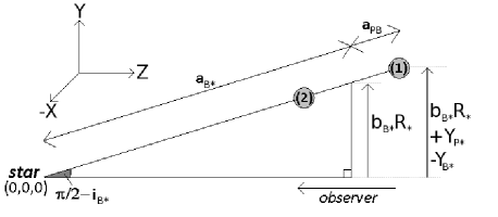
Figure 1.— Cartoon of the TDV-TIP effect. Here, the moon is relaxed into the same orbital plane as the planet’s orbit and causes the planet to experience reflex motion illustrated by the two positions of the planet, (1) and (2). This motion can be seen to cause a change in the apparent impact parameter, which causes a change in the transit duration.

Later, Kipping (2009b) showed that a second transit duration variation (TDV) effect exists, dubbed TDV-TIP, standing for transit-impact-parameter induced TDV. The physical origin of this effect is that if the planet-moon orbital plane is not precisely normal to the sky (which is practically always true), then the planet’s reflex motion must yield a component orthogonal to both the observer’s line-of-sight and the tangent to the planetary motion. This motion leads to periodic variations in the apparent transit impact parameter. Since the transit duration is a strong function of the impact parameter (Seager & Mallén-Ornelas, 2003), then duration variations must follow. The TDV-TIP effect is typically much smaller than the TDV-V (velocity) effect but is strongly enhanced for near-grazing transits. Intrigueingly, TDV-TIP allows one to determine the sense of orbital motion of the moon (i.e. prograde or retrograde) and thus could be a key tool in understanding the origin of the satellite (although such cases require high signal-to-noise). The phase of TDV-TIP is constructive to TDV-V for prograde orbits and destructive for retrograde. The TDV-TIP waveform is shown in Kipping (2011b) to be

$$\mathrm{TDV-TIP} =\tilde{T}_{B}\Bigg{(}\frac{b_{B*}}{1-b_{B*}^{2}}\Bigg{)}\Bigg{(}\frac{a_{SB}M_{S}(1-e_{SB}^{2})}{R_{*}M_{P}}\Bigg{)}\Lambda_{\mathrm{TDV-TIP}},$$ (11)

where

$$\Lambda_{\mathrm{TDV-TIP}} =(1+e_{SB}\cos\nu_{SB})^{-1}\Bigg{[}\sin(\nu_{SB}+\omega_{SB})$$

$$\times[-\cos i_{SB}\sin i_{B*}+\sin i_{SB}\cos i_{B*}\cos\varpi_{SB}]$$

$$+\cos i_{B*}\sin\varpi_{SB}\cos(\omega_{SB}+\nu_{SB})\Bigg{]}.$$ (12)

And the corresponding RMS amplitude is given by

$$\delta_{\mathrm{TDV-TIP}} =\tilde{T}_{B}\Bigg{(}\frac{b_{B*}}{1-b_{B*}^{2}}\Bigg{)}$$

$$\times\Bigg{(}\frac{a_{SB}M_{S}(1-e_{SB}^{2})}{R_{*}M_{P}}\Bigg{)}\sqrt{\frac{\Phi_{\mathrm{TDV-TIP}}}{2\pi}},$$ (13)

where the $\Phi$ term again contains information on the eccentricity and can be found in Kipping (2011b).

It should noted that due to the undersampling issue discussed in regard to TTV, TDV-V and TDV-TIP are simply observed as a global TDV effect. Thus we have two timing observables, TTV and TDV.

3.3. Eclipses Features

A second class of observational effect we can search for is the eclipse of the moon. This eclipse can be either in-front of the star or in-front/behind the planet during the planet-star transit. The former, which we refer to as “auxiliary transits”, is more likely to be detected for moons on wide orbits. The latter, sometimes dubbed “mutual events” (Ragozzine & Holman, 2010; Pál, 2011), is geometrically more probable for moons on close-in orbits. We show examples of each of these types in Figure 2.

Figure 2.— Left panel: transit light curves of a planet with a moon on a wide separation, demonstrating auxiliary transits. Right panel: transit light curves of a planet with a close-in moon, demonstrating mutual events. See Kipping (2011a) for details of the parameters used in these simulations (Figures 7&6 respectively).

Critically, unlike TTV and TDV effects, eclipses are sensitive to the exomoon radius (and not the mass). This presents the opportunity of determining the density of the moon. Further, in an analogous manner to how transiting planets may yield the mean stellar density, $\rho_{*}$, (Seager & Mallén-Ornelas, 2003), transiting moons allow one to measure the mean planetary density directly, $\rho_{P}$, as first shown in Kipping (2010c). Armed with both $\rho_{*}$ and $\rho_{P}$ plus the ratio of the $R_{P}/R_{*}$, one can determine $M_{P}/M_{*}$ (Kipping, 2010c). This powerful trick means that even if no TTV or TDV signal is detected, the eclipses of the moon alone allow one to measure the mass of the exoplanet (assuming $M_{*}$ is known). If radial velocities exist for the system, $M_{*}$ can be measured directly through this technique (Kipping, 2010c). Additionally, the dynamically determined $M_{P}/M_{*}$ can be compared to the RV solution using a-priori value of $M_{*}$ (say from spectroscopy) to ensure consistency.

The ability to weigh planets using moons plays a key role in the HEK project. Candidates with unphysical properties can be quickly rejected as plausible exomoon signals.

4. TARGET SELECTION

4.1. Candidate vs Planet

At the timing of writing, 2326 Kepler transiting candidate planets have been announced (Batalha et al., 2012). However, the public candidate list is only 1235 at the time of writing (Borucki et al., 2011). HEK will employ the most up-to-date list during the development of the project. It should also be noted that included within the candidate list are several candidates which have already been confirmed as bona-fide planets to a high degree of confidence e.g. the Kepler-9 system (Torres et al., 2011).

Despite the progress made in confirming these objects through novel techniques, such as BLENDER (Torres et al., 2004), the vast majority of the planetary candidates remain unconfirmed.

One possible approach might therefore be to only inspect the confirmed planets for exomoons. However, such a strategy is unnecessarily restrictive. The detection of an exomoon would in fact allow one to measure the mass and radius of the planet, as well as the moon (Kipping, 2010c). By modelling these systems, one essentially obtains the same information which is normally provided by radial velocity (RV) or multi-planet transit timing variations (TTV) - the masses. Therefore, exomoon detection is a planetary confirmation tool, in addition to the RV and TTV techniques. Consequently, there is no need to limit ourselves to confirmed planets only and the HEK project will consider all planetary candidates as possible exomoon hosts.

4.2. Target Selection (TS) Overview

Equipped with the capacity of exomoons to confirm planetary candidates, analyzing all of the hundreds of planetary candidates for evidence of exomoons would be the most comprehensive way to proceed. However, practical limitations, such as man-power and computational constraints, make such a task unrealistic. Therefore, we must conduct a target selection (TS) phase. Target selection works by taking the full list of planetary candidates (in our case the KOIs presented in Borucki et al. 2011) and identifying those targets which are of highest priority for more intensive investigation. We have three strategies for target selection, which have some overlap:

1. Visual inspection a subset of planetary candidates for exomoon-like eclipse features (TSV).

2. Automatic filtering of the planetary candidates, based upon system parameters (TSA).

3. Targets of opportunity (TSO).

In some cases, a planetary candidate may fall into more than one category. The identified candidates are then further prioritized by hand. This final stage, which we call target selection prioritization (TSP), is typically done by experience of what constitutes a feasible candidate (see §4.6 for more information).

4.3. Visual Target Selection (TSV) Overview

Visual Target Selection (TSV) is typically conducted by first selecting sub-sample of planetary candidates. This subset is typically selected from some simple parameter constraints such as planet size and semi-major axis. The aim is to allow this subset to have only a weak theoretical prejudice for where to expect a moon. The subset sample size may range from dozens to hundreds of light curves. The light curves are then inspected for features resembling exomoon-like signals, notably:

• Mutual events, preferably with a flat-top (to discriminate from a starspot crossing) e.g. right-panel of Figure 2.

• Auxiliary transits (a second distinct transit feature offset from the primary) e.g. left-panel of Figure 2.

• Repeating anomalies in the light curve of any morphology.

The visual inspection of Kepler photometry has been already been shown to be a useful technique for finding transiting planet candidates (Fischer et al., 2012; Lintott et al., 2012) and here we extend such inspections to hunting for moons too. Whereas TSA relies heavily on the derived parameters of the system (plus an assumed mass-radius relation), TSV is far more ignorant of these values. The benefit of this is that we are able to catch interesting systems which would go missed by TSA due to potential errors in the assumed system parameters (for example from the Kepler Input Catalogue, KIC) or even our theoretical understanding of where moons may reside. TSV systems are later scrutinized to see whether the signal is sufficiently high signal-to-noise, in particular relative to any time correlated noise in the photometry, but this forms part of our final prioritization stage, TSP (see §4.6 for more information).

4.4. Automatic Target Selection (TSA) Overview

TSA works by applying a set of filters which reduce the total planetary candidate list to to a more manageable size. There are several considerations affecting the target selection:

• Availability - Systems for which there exists available photometry.

• Reliability - Systems for which we have reasonable parameters.

• Capability - Systems which are capable of hosting large moons.

• Detectability - Systems which are capable of presenting a detectable moon signal.

TSA leans heavily on the system parameters. Notably, the planetary mass must be essentially guessed based upon the radius. Details on this procedure are presented in §4.4.2.

Stellar parameters of the planetary candidates have been estimated by the Kepler team as part of the Kepler Input Catalogue (KIC), a photometric survey of stars in the Kepler field-of-view designed to identify bright dwarfs as targets for the mission. Brown et al. (2011) describes the estimation of physical parameters, whereby the synthetic spectra of Castelli & Kurucz (2004) are forward-modelled with effective temperature, $T_{\mathrm{eff}}$, surface gravity, log(g), and metallicity, log(Z), as free parameters to match the photometric measurements in the KIC. A relation between luminosity, effective temperature and surface gravity, derived from the stellar evolutionary models computed by Girardi et al. (2000), is used to estimate the stellar masses, which, when combined with log(g), estimates the radii.

Brown et al. (2011) state that the KIC effective temperature and radius estimations are reliable for Sun-like stars, but are “untrustworthy” for stars with $T_{\mathrm{eff}}<3750$ K. To accommodate this possible weakness, TSA is run on both the KIC-only catalogue and a catalogue of KIC plus that of Muirhead et al. (2011), who use near-infrared spectroscopy. These cases will be flagged appropriately. By repeating for both catalogues, we make no decision about which catalogue is the correct one and ensure we do not miss any interesting objects. Any other catalogues which appear will be treated in a similar manner.

4.4.1 Availability

At the time of writing, the only publicly available photometry from Kepler comes from quarters 0, 1, 2 & 3 (Q0, Q1, Q2 & Q3). In all cases, Q1 (33.5d), Q2 (88.7d) and Q3 (89.3d) photometry exists and naturally this will continue to expand as time goes on. Only in some cases is Q0 (9.3d) photometry available. This is because Q0 was technically “calibration” data and originally not expected to be useful scientifically. As a result, the number of sources observed was only 52,496 in Q0 but expanded to 156,097 for Q1. Whilst some sources were dropped from the target list, the majority were kept and thus roughly a third of all sources have Q0 photometry available, in addition to the other quarters.

In most instances, photometry data is currently available in long-cadence (LC) mode only, whereas SC is preferable for our search for reasons described in §4.6. There are three possible exceptions to this rule:

1. A planetary candidate was detected very early on and thus the data was able to be switched to short-cadence (SC) for subsequent observations.

2. The star already had a known exoplanet and thus was observed in SC from the outset.

3. The star was coincidentally pre-selected for asteroseismology and thus was observed in SC for one or more of the three available quarters.

Case 3) is not very useful to us because the subset is rather small. Case 2) is also not useful because the known exoplanets, HAT-P-7b, HAT-11-b and TrES-2b, are all short-period hot-Jupiters which are unlikely to be good exomoon hosts. Case 1) does not guarantee SC data because only 512 targets can be observed in this mode at any one time and the number of planetary candidates exceeds this value significantly (2326; Batalha et al. 2012).

In conclusion, it is generally unlikely that a potentially interesting target (for exomoon hunting) will have any useful SC data available at the start of the HEK project and this represents a major limitation on our capabilities. Those that do are highly valuable to HEK, during this stage of the project, given that SC data strongly enhances our capability to detect exomoons. As we mentioned before though, more quarters are becoming public over time, including potentially much more SC data, and thus the effectiveness of our program is likely to improve significantly over time.

To look for exomoons, we require systems where at least three transits have been observed. This is because three transits represents the minimum number for timing deviations to be inferred. Two transits only introduces a total degeneracy between the orbital period of the planet and the transit timing variation (TTV) amplitude. Let us denote the total baseline of data as $B$ days and assume optimistically that Q0 exists. In order to “guarantee” three transits have been recorded, we set the maximum allowed orbital period to be $P_{P}\leq B/4$, which is our first filter.

4.4.2 Reliability

Kepler measures the ratio-of-radii of planetary candidates, rather than their absolute radii. From photometric measurements discussed in Brown et al. (2011), the Kepler input catalogue (KIC) contains estimated masses and radii for all of the host stars. Therefore, the planetary radii can be determined to a reasonable degree of reliability.

However, one of the key parameters in both predicting the feasibility of a moon around a planet and the detectability is the mass of the host planet, $M_{P}$ (particularly for computing the Hill sphere). Kepler cannot measure the masses of these objects, except in some extreme cases where ellipsoidal variations (Mislis et al., 2011) or TTVs exist (Agol et al., 2005).

The maximum allowed exomoon mass around a planet scales as $M_{S,\mathrm{max}}\sim M_{P}^{8/3}$ (see Equation 1). If we overestimate this value, we will waste time looking at systems where moons cannot exist. If we underestimate this value, we will miss some potentially interesting candidates. However, the number of candidates is large and we can afford to miss some objects for the sake of focussing on the very best candidates. Therefore, we choose to provide a minimum estimate of $M_{P}$.

Planets are frequently broken up into three regimes: i) Super-Earths ii) Neptunes iii) Jupiters. For a Super-Earth, the mass-scaling relationship is arguably the most predictable relative to the other two regimes, due to the known properties of rock under pressure. The precise location of the boundary between a gas/ice giant and a rocky Super-Earth, and the conditions under which such a boundary varies, is empirically a subject in its infancy. However, models of the growth of a protoplanet’s envelope suggest a critical mass of $M_{P}\sim 20$ $M_{\oplus}$ (see review article D’Angelo et al. 2010), whereafter the envelope growth timescale rapidly diminishes by orders of magnitude. This suggests that the maximum radius of a rocky planet is $R_{P}\sim 2$ $R_{\oplus}$, using the scaling relation of Valencia et al. (2006). This boundary is consistent with that adopted in other works, such as Borucki et al. (2011). Therefore, if a planet has $R_{P}\lesssim 2\,R_{\oplus}$, we consider it more likely to be icy/rocky rather than gaseous. The assumed mass of the Super-Earth is calculated using the Valencia et al. (2006) relation $(R_{P}/R_{\oplus})\sim(M_{P}/M_{\oplus})^{0.27}$. We stress that this assumption is only used for target selection and is not adopted in the actual fits or system analyses.

The definition of a Neptune is somewhat more tenuous but we use the same definition as that of Borucki et al. (2011) - planets which satisfy $2\,R_{\oplus}<R_{P}<6\,R_{\oplus}$. Transiting “Neptunes” are in short supply in the exoplanet literature, especially those with well-determined densities (SNR$>3$). Figure 3 shows bulk density versus the radius of the six exoplanets which satisfy this criteria. Systems parameters are taken from Gillon et al. (2011), Kundurthy et al. (2011), Fossey et al. (2012), Bakos et al. (2009), Henry et al. (2011) and Cochran et al. (2011) for 55-Cnc-e, GJ 1214b, GJ 436b, HAT-P-11b, HD 97658b and Kepler-18c respectively.

From these, four out of the six settle around an approximately common density close to that of Neptune and Uranus of $\bar{\rho}_{P}=1.7\pm 0.3$ g cm^-3 (where the uncertainty is the standard deviation of these four). The median of all six is 1.5 g cm^-3. 55-Cnc-e has a much higher density of $4.0_{-0.3}^{+0.5}$ g cm^-3, possibly due to its close proximity (in radius) to the Super-Earth/Neptune boundary ($R_{P}=2.17\pm 0.10$ $R_{\oplus}$) and is ostensibly not a typical member of the $2\rightarrow 6$ $R_{\oplus}$ category. Similarly, Kepler-18c is the largest radii planet ($R_{P}=5.5\pm 0.3$,$R_{\oplus}$) close to the Neptune/Jupiter boundary of 6 $R_{\oplus}$ and exhibits a much lower density of $0.6\pm 0.1$ g cm^-3, and thus may not be typical either.

We therefore decide to settle on an assumed density of $1.7$ g cm^-3 to get an assumed planetary mass in TSA. The function of this assumed mass will be primarily in computing the maximum allowed exomoon mass and a generous margin will be assigned to this calculation to account for the fact we have made such a broad approximation (as will be discussed later). As before, this again only used for TSA and not employed in the final analyses.

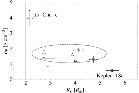
Figure 3.— Bulk densities of all known transiting exoplanets in the “Neptune” regime. We only show planets with densities determined with SNR$>3$. Triangles mark the position of Neptune and Uranus for context. Vertical grid lines mark the Super-Earth and Jupiter boundaries, as defined by Borucki et al. (2011). We mark the location of the somewhat anomalous 55-Cnc-e and Kepler-18c. The gray ellipse represents a 2-$\sigma$ bound of the bulk of points yielding an approximately uniform density of $1.7\pm 0.3$ g cm^-3.

Planets above the $6\,R_{\oplus}$ boundary show much greater variation in density, going from extrema of $0.122_{-0.042}^{+0.072}$ g cm^-3 for WASP-17b (Anderson et al., 2010) to $26.4\pm 5.6$ g cm^-3 for CoRoT-3b (Deleuil et al., 2008). At this point, we consider the reliability of any mass-radius relation to be untenable and thus we add the filter than any planet of radius $R_{P}>6$ $R_{\oplus}$ are not considered. This also helps in the exomoon detection too, since smaller planets present larger mutual events with a putative companion (Kipping, 2011a).

It is important to stress that in all cases that the assumed masses are only used for target selection purposes and will not be adopted as final values in the actual system analyses.

4.4.3 Capability

For each Kepler candidate, we need to know the capability of the planet to host a moon. The maximum allowed exomoon mass from Equation 1 (Barnes & O’Brien, 2002) offers a useful way of accomplishing this. We assume a retrograde moon so that the maximum allowed semi-major axis of the moon’s orbit is 93.09% of the Hill radius (i.e. $\mathfrak{D}_{\mathrm{max}}=0.9309$).

To compute the maximum allowed moon mass, we use the system parameters presented in Borucki et al. (2011) or more recent results where available. As discussed earlier, the planetary mass is assumed following some simple scaling rules. Finally, we assume the same Jovian-like tidal dissipation parameters as that used by Barnes & O’Brien (2002): specifically $Q_{P}=10^{5}$ and $k_{2p}=0.51$. The $k_{2p}$ value is that for a $n=1$ polytrope (Hubbard, 1984) and the $Q_{P}$ factor is consistent with estimates for Jupiter (Goldreich & Soter, 1966). This then allows us to compute the maximum allowed exomoon mass, assuming $\mathbb{T}=5$ Gyr, using Equation 1, taken from Barnes & O’Brien (2002).

It is important to realize this calculation is intended to only point the way towards potentially interesting targets. It is not intended to be the final determination of this value, which is simply not possible with the current information available.

Accordingly, we exclude all candidates for which the maximum moon mass is below $10$ $M_{\oplus}$. This high limit is deliberately an overestimate to allow for the number of assumptions and approximations made thus far. We further exclude planets with $a_{B*}<0.1$ AU based upon the arguments given in §2.5 and (Namouni, 2010).

4.4.4 Detectability

In order to make an exomoon detection, we require a mass and radius. The timing amplitudes, which yield the exomoon mass, depend upon the configuration of the system but the eclipse amplitude, yielding the exomoon radius, has a far weaker correlation to these terms. The eclipse amplitude is approximately given by $(R_{S}/R_{*})^{2}$ and thus for any given target we should be able to easily estimate the eclipse signal of an Earth-sized moon i.e. $(R_{\oplus}/R_{*})^{2}$.

We may also estimate the SNR over a 6.5-hour integration time by simply dividing the exomoon eclipse depth by the CDPP values presented in Borucki et al. (2011). We filter all out results where SNR$<1$ for a single event.

4.5. Opportunity Target Selection (TSO) Overview

Additionally, we will consider “targets of opportunity” for special objects of interest. We envision these will typically be confirmed, published Kepler exoplanets. These targets offer numerous advantages in that the entire photometric time series used in the discovery paper is usually available (i.e. many more quarters than normal), SC data is often available, the planet is known to be genuine and frequently follow-up information such as spectroscopy, radial velocities or even asteroseismology are usually available too. We envision that these TSO targets would be typically selected for HEK analysis because they have special significance (e.g. are in the habitable-zone).

4.6. Target Selection Prioritization (TSP) Overview

The prioritization stage is the process of selecting just a few targets out of the candidates found by the TSA, TSV and TSO stages. TSP is typically done using detailed light curve inspection, experience of what constitutes a viable signal and other factors.

For example the availability of short-cadence (SC) data is a key TSP factor, due to the improved sensitivity relative to long-cadence (LC) data. This is because many of the exomoon features induced on the light curve can occur on timescales shorter than 30 minutes and thus would be lost in the LC data. Further, SC data yields higher resolution of the ingress/egress of the planetary transit which thus yields a tighter determination of the planetary parameters (Kipping, 2010b). With lower uncertainty on the planetary signal, we are naturally able to more easily distinguish exomoon signals. Therefore, targets with even partial SC data are strongly preferred to those with exclusively LC photometry.

5. FITTING

5.1. Modelling Strategy: LUNA

Modelling the eclipses of planet-moon systems is non-trivial, if one wishes to retain analytic expressions. The advantages of an analytic model are manifold, allowing CPU intensive fitting techniques (e.g. Monte Carlo methods) to fully explore the complex parameter space. The requirement for an analytic algorithm excludes the methods presented in Simon et al. (2009), Sato & Asada (2009), Deeg (2009), and Tusnski & Valio (2011).

The most significant challenge, in terms of analytic modelling, is when the planet, moon and star all partially overlap. The analytic solution for the area of overlap of three circles was only recently found by Fewell (2006) and this discovery allowed for the first time an exomoon code which could be totally analytic in nature.

Kipping (2011a) presented an algorithm to this end, dubbed LUNA, which dynamically models the planet-moon motion and utilizes the Fewell (2006) solution (plus numerous new solutions derived in Kipping 2011a) to produce simulated light curves for moons. The code uses quadratic limb darkening and runs almost as fast as generating a planet signal by itself (i.e. the code of Mandel & Agol 2002). As a result, LUNA is easily implemented with Monte Carlo based fitting techniques. Further, the dynamical component of LUNA means that effects such as TTV, TDV-TIP and TDV-V are all inherently accounted for, plus other previously unconsidered effects such as ingress/egress asymmetry. LUNA is a potent weapon in exomoon detection.

We note that another analytic algorithm capable of modelling exomoon eclipses has appeared recently in Pál (2011). However, the HEK project will make use of LUNA alone, since this already satisfies all of our requirements.

LUNA also features several other light curve analysis techniques developed recently, such as accounting for the finite integration time using selective resampling (Kipping, 2010b) and accounting for blended/third-light using the methodology of Kipping & Tinetti (2010).

5.2. Detection Strategy: Bayesian Model Selection

The process of making a detection of any physical phenomenon is essentially an exercise in model selection. In our case, this is most simply described by comparing how well the data are explained by a planet-only model (the null hypothesis) versus a planet-with-moon model.

The Bayesian framework is a very powerful basis for these model comparisons, allowing the observer to incorporate prior knowledge (such as the allowed physical bounds of various parameters) and naturally include “Occam’s razor” as a way of penalizing overly-complicated models. Whilst various information criterion have been proposed for performing model selection, the use of Bayesian evidence has emerged as the metric of choice to perform model comparisons (Liddle et al., 2007).

Bayesian inference methods provide a consistent approach to the estimation of a set parameters $\mathbf{\Theta}$ in a model $\mathcal{M}$ for the data $\mathbf{D}$. Bayes’ theorem states that

$$\mathrm{Pr}(\mathbf{\Theta}|\mathbf{D},\mathcal{M}) =\frac{\mathrm{Pr}(\mathbf{D}|\mathbf{\Theta},\mathcal{M})\mathrm{Pr}(\mathbf{\Theta}|\mathcal{M})}{\mathrm{Pr}(\mathbf{D}|\mathcal{M})},$$ (14)

where $\mathrm{Pr}(\mathbf{\Theta}|\mathbf{D},\mathcal{M})=\mathcal{P}(\mathbf{\Theta})$ is the posterior probability distribution of the parameters, $\mathrm{Pr}(\mathbf{D}|\mathbf{\Theta},\mathcal{M})=\mathcal{L}(\mathbf{\Theta})$ is the likelihood, $\mathrm{Pr}(\mathbf{\Theta}|\mathcal{M})=\pi(\mathbf{\Theta})$ is the prior, and $\mathrm{Pr}(\mathbf{D}|\mathcal{M})=\mathcal{Z}$ is the Bayesian evidence.

The evidence can be understood to be simply the factor required to normalize the posterior over $\mathbf{\Theta}$, so that

$$\mathcal{Z} =\int\mathcal{L}(\mathbf{\Theta})\pi(\mathbf{\Theta})\,\mathrm{d}^{D}\mathbf{\Theta},$$ (15)

where $D$ is the dimensionality of the parameter space. Since the evidence is the average of the likelihood over the prior, Occam’s razor is inherently included. Therefore, a simpler theory with more compact parameter space will yield a larger evidence than a more intricate theory. Model selection between two competing theories, $\mathcal{M}_{0}$ and $\mathcal{M}_{1}$ can be decided by comparing their respective posterior probabilities, for the given data, via

$$\frac{\mathrm{Pr}(\mathcal{M}_{1}|\mathbf{D})}{\mathrm{Pr}(\mathcal{M}_{0}|\mathbf{D})} =\frac{\mathcal{Z}_{1}}{\mathcal{Z}_{0}}\frac{\mathrm{Pr}(\mathcal{M}_{1})}{\mathrm{Pr}(\mathcal{M}_{0})},$$ (16)

where $\mathrm{Pr}(\mathcal{M}_{1})/\mathrm{Pr}(\mathcal{M}_{0})$ is the a-priori probability ratio for the two models, typically set to unity but occasionally requires more thought. In this way, the odds ratio of a planet-with-moon model can be assessed, relative to a planet-only model. Defining the Bayes’ factor as $\mathcal{B}=\mathcal{Z}_{1}/\mathcal{Z}_{0}$, $|\log\mathcal{B}|>6$ indicates a $>3$ $\sigma$ detection, $|\log\mathcal{B}|>10$ indicates $>4$ $\sigma$ and $|\log\mathcal{B}|>15$ indicates $>5$ $\sigma$.

5.3. Fitting Strategy: MultiNest

In the exoplanet literature, Markov Chain Monte Carlo (MCMC) techniques have emerged as the favoured tool for fitting transit light curves. However, the technique is primarily for parameter estimation and does not natively yield the Bayesian evidence. Whilst techniques such as thermodynamic integration (e.g. see Ó Ruanaidh & Fitzgerald 2011) can get round this problem, it comes at the cost of great computational expense.

5.3.1 Nested sampling

Nested sampling (Skilling, 2004) is a Monte Carlo method which puts the calculation of the Bayesian evidence in a central role, but also produces posterior inferences as a by-product. Nested sampling is generally considerably more efficient than MCMC methods. For example, in cosmological applications, Mukherjee et al. (2006) showed that their implementation of the method requires a factor of $\sim 100$ fewer posterior evaluations than thermodynamic integration.

A full discussion of nested sampling is given in Skilling (2004) and Feroz et al. (2009a). We here provide a brief description, following the notation of Feroz et al. (2009a), for the purposes of conceptually illustrating the technique.

Nested sampling takes advantage of the relationship between the likelihood and the prior volume to transform the multidimensional evidence integral (Equation 15) into a more manageable one-dimensional integral. The “prior volume” X is defined by $\mathrm{d}X=\pi(\Theta)\mathrm{d}^{D}\Theta$, such that

$$X(\lambda)=\int_{\mathcal{L}(\mathbf{\Theta})>\lambda}\pi(\mathbf{\Theta})\,\,\mathrm{d}^{D}\mathbf{\Theta},$$ (17)

where the integral extends over the region(s) of parameter space contained within the iso-likelihood contour $\mathcal{L}(\mathbf{\Theta})=\lambda$. One may then re-write the evidence integral of Equation 15 in the form

$$\mathcal{Z}=\int_{0}^{1}\mathcal{L}(X)\,\,\mathrm{d}X,$$ (18)

where $\mathcal{L}(X)$, which is the inverse of Equation 17, is a monotonically decreasing and continuous function of $X$. Consequently, if one can evaluate a series of $M$ likelihoods via $\mathcal{L}_{i}=\mathcal{L}(X_{i})$, where $X_{i}$ is a sequence of decreasing volumes from unity ($X_{0}$) to zero ($X_{M}$) as shown schematically in Figure 4, then the evidence may be approximated numerically as a weighted sum using

$$\mathcal{Z}=\sum_{i=1}^{M}\mathcal{L}_{i}w_{i}.$$ (19)

The weights may be computed using the trapezium rule, $w_{i}=\frac{1}{2}(X_{i-1}-X_{i+1})$. The algorithm works by casting a net of $N$ “active” points across the initial prior space. The active point with the lowest likelihood is removed (made “inactive”) and a new replacement point is generated such that its likelihood is higher than this rejected value. As the algorithm progresses, it travels through nested shells of likelihood as the prior volume is reduced. The routine is terminated once the evidence is computed to some tolerance precision, typically 0.5 in log-evidence. Upon termination, parameter posteriors may also be computed using the active and inactive points.

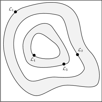
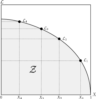
Figure 4.— Cartoon illustrating (a) the posterior of a two dimensional problem; and (b) the transformed $\mathcal{L}(X)$ function where the prior volumes $X_{i}$ are associated with each likelihood $\mathcal{L}_{i}$.

5.3.2 Multimodal nested sampling

Multimodal nested sampling is an implementation of nested sampling to both account for multiple modes and achieve efficient sampling via the use of the “simultaneous ellipsoidal sampling” method, described in Feroz et al. (2007). A publicly available version of the algorithm, dubbed MultiNest, is available. We direct the reader to Feroz et al. (2009a) for a description of the algorithm and its use (including several toy examples).

To date, applications of the technique have been mostly limited to cosmology, gravitational wave detection and particle physics (e.g. see Vegetti et al. 2010, Feroz et al. 2009b and Abdussalam et al. 2010 respectively). Recently however, Feroz et al. (2011) demonstrated the first application of the technique to radial velocity data for detecting extrasolar planets. Here, we briefly discuss our application of MultiNest to transit light curve fitting (we note that a detailed study of MultiNest for fitting transits is currently in preparation by Balan et al., personal communication).

5.3.3 Combining MultiNest and LUNA

Nested sampling allows one to compute the Bayesian evidence of a model fit at a much lower computational cost than using thermodynamic integration with MCMC techniques. However, there are many other advantages of employing MultiNest with LUNA, rather than an MCMC.

The most simple and common flavour of MCMC is the Metropolis-Hastings algorithm, widely used in the recent exoplanet literature. With a unimodal likelihood function, this technique is effective and robust, capable of identifying the single minimum even when the initial starting point of the chain is widely separated from this minimum. However, multimodal distributions are extremely problematic. If the spacing between two modes is much greater than the width of the proposal distribution, then the MCMC will take an inordinate amount of time to cross over and practically speaking the MCMC is stuck in a local minimum. For a planet-only model, a unimodal likelihood distribution is generally expected but a planet-with-moon model exhibits many modes, especially due to harmonic power in the TTVs and TDVs (Kipping, 2009a).

MultiNest comprehensively searches the entire prior volume identifying all minima and thus is not affected by this problem. We point out, however, that more elaborate flavours of MCMC can still find the global minimum but at further computational cost. Techniques such as parallel tempering (Geyer, 1991), differential evolution (Ter Braak, 2006) and genetic crossovers (Gregory, 2009) can be appended into the MCMC methodology.

To implement LUNA with MultiNest, we simply need to define a likelihood function. MultiNest calls LUNA for each active point and LUNA returns a likelihood value of the point. It is only at this point where communication between the two algorithms occurs and so is the only outstanding problem in implementing a combination of MultiNest with LUNA. For quiet stars, the noise properties of the photometry is nearly perfectly Gaussian (Kipping & Bakos, 2011b). For Gaussian uncorrelated noise, the likelihood function may be simply defined as

$$\mathcal{L}(\mathbf{\Theta}) =\prod_{i=1}^{N}\frac{1}{\sqrt{2\pi\sigma_{i}^{2}}}\exp\Big{[}-\frac{(f_{\mathrm{obs},i}-f_{\mathrm{mod},i}(\mathbf{\Theta}))^{2}}{2\sigma_{i}^{2}}\Big{]},$$ (20)

where $f_{\mathrm{obs},i}$ is the observed flux, $f_{\mathrm{mod},i}(\mathbf{\Theta})$ is the model flux returned by LUNA, and $\sigma_{i}$ is the photometric uncertainty.

In cases where correlated noise constitutes a significant component of the noise budget, then the likelihood function may be modified accordingly. For example, Carter et al. (2008) present a wavelet-based likelihood function to compensate for time-correlated noise.

5.4. Choosing the Parameters

The parameter set for the fitting procedure should be physically-motivated so that well-defined boundary conditions may be imposed, have a uniform prior and exhibit as small as possible mutual correlations with the other fitting terms. Unless the algorithm is imposed with non-uniform priors, the choice of parameters often defines the choice of priors too.

5.4.1 Planet parameters

The choice of the parameter set for fitting a planet-only model is a subject which has been investigated in numerous papers in the exoplanet literature (e.g. see Carter et al. 2008 and Kipping 2010a). The transit of a spherical planet on a circular orbit across a uniformly bright, spherical star is described by just four parameters, which is expected given the near-trapezoidal nature of the light curve. These parameters are $\{\tau_{B*},p,(a_{B*}/R_{*}),b_{B*}\}$, where $\tau_{B*}$ is the time of the transit minimum of the planet’s barycentre across the star, $p$ is the ratio-of-radii (i.e. $R_{P}/R_{*}$), $(a_{B*}/R_{*})$ is the orbital semi-major axis of the planet’s barycentre around the star in units of the stellar radius and $b_{B*}=(a_{B*}/R_{*})\cos i_{B*}$ (where $i_{B*}$ is the orbital inclination of the planet’s barycentre around the star). Multiple transits allows one to fit for the orbital period, $P_{B*}$, as well. Of these terms, only $(a_{B*}/R_{*})$ and $b_{B*}$ are problematic, due to their very strong mutual correlation. Further, whilst $b_{B*}$ is bound to be $0<b_{B*}<1$ for fully transiting planets, $(a_{B*}/R_{*})$ lies within the range $0<(a_{B*}/R_{*})<\infty$ and is therefore not appropriate for a uniformly distributed prior.

Carter et al. (2008) have suggested using transit duration related replacements for $(a_{B*}/R_{*})$ and $b_{B*}$ to reduce the mutual correlation, but these also have essentially unbounded upper limits. Kipping et al. (2012) have suggested replacing $(a_{B*}/R_{*})$ with $[\rho_{*}^{\mathrm{circ}}]^{2/3}$ (the mean stellar density of a spherical star assuming a circular orbit, to the power of two-thirds). Besides from reducing the correlation to $b_{B*}$, the bounded limits are far better known if we assume the planet is orbiting a main-sequence star and impose an upper limit on the eccentricity. Further, the posteriors may be used directly to conduct multibody asteroseismology profiling (MAP) analysis, which is useful in constraining eccentricity in multiple systems (Kipping et al., 2012). Thus, we choose to use $\{\tau_{B*},p,[\rho_{*}^{\mathrm{circ}}]^{2/3},b_{B*},P_{B*}\}$, and adopt

$$\rho_{*}^{\mathrm{circ}} \simeq\frac{3\pi[(a_{B*}/R_{*})^{\mathrm{circ}}]^{3}}{GP_{B*}^{2}},$$ (21)

where we have assumed $M_{P}\ll M_{*}$ to simplify the expression. To allow for non-circular orbits, we fit for $\sqrt{e_{B*}}\sin\omega_{B*}$ and $\sqrt{e_{B*}}\cos\omega_{B*}$, which maintain uniform priors in $e_{B*}$ and $\omega_{B*}$ but generally exhibit lower mutual correlations than fitting for $e$ and $\omega$ directly. Limb darkening may be included by adopting a quadratic limb darkening law characterized by $u_{1}$ and $u_{2}$ limb darkening coefficients. These are constrained to lie within the range $0<u_{1}+u_{2}<1$ and $u_{1}>0$ (Carter et al., 2009). An upper bound on $u_{1}$ may be estimated by inspection of a typical set of coefficients from stellar atmopshere models. For example, Claret (2000) have a maximum $u_{1}$ coefficient of 1.4336 across all listed $T_{\mathrm{eff}}$, $\log g$, etc values and across all bandpasses. We use $u_{1}<2$ as a conservative upper limit.

Finally, we allow each transit epoch to have its own unique out-of-transit baseline normalization factor, OOT. These OOT values are represented by the vector OOT are typically not presented in final results tables, but are available upon request.

5.4.2 Moon parameters

For a planet-with-moon model, a similar set of parameter arises, but with subtle differences. For example, the inclination of the moon around the planet-moon barycentre, $i_{SB}$, can be redefined in terms of an impact parameter as before (e.g. $b_{SB}=(a_{SB}/R_{*})\cos i_{SB}$), but the $0<b_{SB}<1$ bound no longer applies, rather we have $-\infty<b_{SB}<\infty$. Inclination follows $0<i_{SB}<\pi$ for prograde moons and $\pi<i_{SB}<2\pi$ for retrograde moons. Since neither $\arcsin$ nor $\arccos$ are unique over the range $0$ to $2\pi$ and the light curve is not symmetric at any boundary, then neither is appropriate for exomoons. Instead, we simply use $i_{SB}$. We may also use the full range of $0$ to $2\pi$ for the bounds to allow both prograde and retrograde solutions to be sought. The same is true for the longitude of the ascending node, $\Omega_{SB}$, which is bound by $-\pi/2<\Omega_{SB}<\pi/2$. Allowing for inclined moons is important since an exoplanet’s obliquity is not expected to tidally decay except for orbits relatively close to the star (Heller et al., 2011).

Eccentricity terms such as $e_{SB}$ and $\omega_{SB}$ may be fitted either directly or using the replacements $\sqrt{e_{SB}}\sin\omega_{SB}$ and $\sqrt{e_{SB}}\cos\omega_{SB}$ (which still maintains a uniform prior in both terms). The latter option tends to be less correlated and thus preferable.

$P_{SB}$ may be fitted either directly or fitting for $\log P_{SB}$ to impose a Jeffrey’s prior. In either case, the parameter may range from a moon grazing the planetary surface ($\sim$ hours timescale) to being at exactly one Hill radius, occurring at $P_{SB}\simeq P_{B*}/\sqrt{3}$ (Kipping, 2009a). The phase angle of the moon, $\phi_{SB}$, is simply fitted directly within the range of $0$ to $2\pi$. $(a_{SB}/R_{*})$ raises similar problems as was encountered with facing $(a_{B*}/R_{*})$. However, we may again make use of the same density trick; namely, through Kepler’s Third Law we have

$$\rho_{P} \simeq\frac{3\pi(a_{SB}/R_{*})^{3}}{GP_{SB}^{2}p^{3}},$$ (22)

where we have assumed $M_{S}\ll M_{P}$ to simplify the expression. Physically motivated and sensible bounds on $\rho_{P}$ may be easily estimated, in addition to $P_{SB}$ and $p$. It is convenient to fit for the mass and radius ratios directly using $M_{S}/M_{P}$ and $R_{S}/R_{P}$, since the boundary conditions are given by zero to unity in both cases. Since the mass and radii ratios are related to the density ratio, we choose to keep the planetary density analogous to the stellar density by putting to the power of two-thirds again i.e. we fit for $\rho_{P}^{2/3}$. Table 1 summarizes the priors used.

Table 1Planet-moon parameters used in light curve fits and their associated priors.

Parameter	Prior
Planet Parameters
$p$	$\mathcal{U}\{0,0.25\}$
$[\rho_{*}^{\mathrm{circ}}]^{2/3}$  [$\mathrm{kg}^{2/3}$ $\mathrm{m}^{-2}$]	$\mathcal{U}\{[\rho_{*}^{\mathrm{circ,min}}]^{2/3},[\rho_{*}^{\mathrm{circ,max}}]^{2/3}\}$
$b_{B*}$	$\mathcal{U}\{0,1\}$
$P_{B*}$  $[\mathrm{days}]$	$\mathcal{U}\{P_{B*}^{\mathrm{min}},P_{B*}^{\mathrm{max}}\}$
$\tau_{B*}$  [BJDTDB]	$\mathcal{U}\{\tau_{B*}^{\mathrm{min}},\tau_{B*}^{\mathrm{max}}\}$
$\sqrt{e_{B*}}\cos\omega_{B*}$	$\mathcal{U}\{-1,1\}$
$\sqrt{e_{B*}}\sin\omega_{B*}$	$\mathcal{U}\{-1,1\}$
$(u_{1}+u_{2})$	$\mathcal{U}\{0,1\}$
$u_{1}$	$\mathcal{U}\{0,2\}$
OOT	$\mathcal{U}\{0.95,1.05\}$
Moon Parameters
$R_{S}/R_{P}$	$\mathcal{U}\{0,1\}$
$M_{S}/M_{P}$	$\mathcal{U}\{0,1\}$
$[\rho_{P}]^{2/3}$  [$\mathrm{kg}^{2/3}$ $\mathrm{m}^{-2}$]	$\mathcal{U}\{[\rho_{P}^{\mathrm{min}}]^{2/3},[\rho_{P}^{\mathrm{max}}]^{2/3}\}$
$i_{SB}$  [rads]	$\mathcal{U}\{0,2\pi\}$
$\Omega_{SB}$  [rads]	$\mathcal{U}\{-\pi/2,\pi/2\}$
$P_{SB}$  $[\mathrm{days}]$	$\mathcal{U}\{0.083,P_{B*}/\sqrt{3}\}$
$\phi_{SB}$  [rads]	$\mathcal{U}\{0,2\pi\}$
$\sqrt{e_{SB}}\cos\omega_{SB}$	$\mathcal{U}\{-1,1\}$
$\sqrt{e_{SB}}\sin\omega_{SB}$	$\mathcal{U}\{-1,1\}$

6. VETTING

There are two principal signals we are trying to detect: timing variations and eclipse effects. Timing variations which could mimic moons can be induced by other perturbing bodies or even stellar activity. Similarly, light curve distortions similar in morphology to mutual events can be induced by star spot crossings. However, it should be noted that out-of-transit companion eclipses are much harder to mimic.

Nevertheless, there is clearly a need to vet exomoon signals as being genuine or not, in the same way candidate planets must be vetted. There are numerous tools at our disposal to aid in this procedure. Most generally, we follow the six detection criteria of Kipping (2011b) (see Chapter 1, §4 for details):

• Statistically significant

• Systematic errors dealt with

• Physically plausible claim

• Not a suspicious period(s)

• Consistent instrumentation

• Avoid large systematics (e.g. highly active stars)

Vetting is essentially the act of proposing alternative models which can perhaps equally well, or even better, explain the observations. Thus we are considering additional models $\mathcal{M}_{2},\mathcal{M}_{3},\mathcal{M}_{4}$, etc and computing their evidences relative to that of $\mathcal{M}_{1}$, the planet-with-moon model. However, we note that in some cases, formally computing the evidence of an alternative model may not be necessary since it may immediately obvious that the observations cannot be caused by the alternative model in question.

6.1. Weighing Tools

The most powerful tool at our disposal for vetting will be the derived densities from the light curve fits. As stated in §3.3 & 4.1, exomoon systems allow one to measure the bulk density of the star, planet and moon all through photometry alone (Kipping, 2010c). If one also has some radial velocity data, then the absolute dimensions of all three bodies can be determined using Kepler’s Third Law.

If the moon is not genuine, but caused by some false-positive or even just residual noise in the data, then it is highly improbable that these values will come out to be remotely physical. Thus, by bounding the prior volume to only physically plausible values (as discussed in §5.4), we forcibly exclude the vast majority of false positives.

In most cases, we will not have a determination of the radial velocity semi-amplitude, $K_{*}$, at our disposal due to the faintness of the Kepler targets (although we may have an upper limit). Even without $K_{*}$, we still directly measure $\rho_{*}$, $\rho_{P}$ and $\rho_{S}$. Using the some reasonable estimate for $M_{*}$ and $R_{*}$, allows for the dimensions of all three bodies to be determined.

6.2. Starspot Crossings

Starspot crossings can mimic exomoon-like mutual events. There are several ways in which they differ though. First of all, a starspot crossing tends to be V-shaped (e.g. see Sanchis-Ojeda & Winn 2011) due to the fact that the spots are typically greater than or approximately equal to the size of the transiting planet. In contrast, exomoon signatures should usually be flat-topped, but can in some more non-aligned geometries be V-shaped. Nevertheless, a flat-topped mutual event would be a strong indicator that the event was due to a moon rather than starspot crossing.

Secondly, starspots have chromatic variations whereas a mutual event should not. Thus there is the possibility of conducting follow-up observations from the ground to interrogate this hypothesis. Thirdly, starspots should track across the stellar surface with a speed determined by the rotational period of the host star, $P_{*,\mathrm{rot}}$. This term is usually determinable from the photometry alone, should the star be sufficiently active.

Since an auxiliary transit outside of the main transit event is much more difficult to mimic through stellar activity, these events will undoubtedly be more easily detected. These events tend to be associated with moons on large separations such as a wide-captured retrograde moon and thus we anticipate that HEK may have a detection bias in this regard.

However, starspots are unlikely to be both well-modelled by an exomoon-fit and produce physically plausible densities for the star, planet and moon. This is because starspots tend to produce very strong eclipse features but only weak timing artifacts. For example, HAT-P-11b transits a heavily spotted star exhibiting eclipse features of up to 1-2 mmag in depth (Sanchis-Ojeda & Winn, 2011) but timing deviations of $\lesssim 30$ seconds (Deming et al., 2011). The absence of significant timing variations would cause the planet-with-moon fit to favour an implausibly low density moon. Thus, the weighing tools will be a most common test for the presence of spots.

6.3. Transit Timing Analysis

Transit timing variations (TTVs) are induced in both resonant (Agol et al., 2005; Holman & Murray, 2005) and non-resonant systems (Nesvorný & Beaugé, 2010). One possible model to explain a candidate moon system would be a transiting planet influenced by an unseen perturbing planet, $\mathcal{M}_{2}$. The evidence of this model may be computed by allowing each transit epoch to have its own unique time of transit minimum, $\tau_{B*,i}$, and proceeding as before with the planet-only fit.

Aside from producing an evidence value more favourable than the planet-with-moon fit, model $\mathcal{M}_{2}$ must correspond to a physically plausible scenario. To investigate this, we will use the TTV-inversion code developed by Nesvorný & Beaugé (2010), ttvim.f, to explore the range of plausible perturbers. If no plausible perturbers can fit the transit times, then model $\mathcal{M}_{2}$ will have a negligible prior probability i.e. $\mathrm{Pr}(\mathcal{M}_{2})\rightarrow 0$. Such an instance would thus favour the planet-with-moon model over the perturber model. If the perturber is both feasible and of comparable evidence to the moon-model, then one may search the photometric time series for transits of the other planet directly.

The same process may be repeated for other sources of TTVs too, such as the model of a Trojan perturber (Ford & Holman, 2007), model $\mathcal{M}_{3}$. For such scenarios, transits of the Trojan(s) can also be sought (e.g. Kipping & Bakos 2011a).

6.4. Radial Velocities

Whenever possible, the HEK project will seek to obtain radial velocities of the target systems to confirm both the planetary and lunar nature of the candidates. Since TSA targets only sub-Jupiters on moderate-to-long periods, the expected RV amplitudes will be typically $\lesssim 10$ m/s. Detecting this signal would allow us to both confirm the candidate and determine the absolute dimensions of the system. However, excluding RV amplitudes above a certain threshold is also useful in eliminating false positives.

Aside from dynamically weighing the system, we anticipate precise radial velocities will be very useful in locating the correct orbital period of the moon. As discussed earlier and in Kipping (2009a), the timing signals can be fitted by a forest of harmonic orbital periods due to the undersampled nature of our observations. A very strong eclipse signal can remove this degeneracy, as can enforcing coplanarity, but if either of these is not possible, we are left with a forest of harmonics. Each period yields a unique $\rho_{P}$ and thus unique light curve derived $M_{P}/M_{*}$. For example, a synthetic example shown later in §7.2 finds two harmonic modes with derived $\rho_{P}$ values differing by more than a factor of two. If precision radial velocities can infer $M_{P}/M_{*}$ independently, then the correct harmonic is empirically determined. Thus, systems with indistinguishable harmonic modes will be prioritized for radial velocity follow-up.

7. Worked Examples

7.1. Null Example: HZ Neptune around an M2 star

As a null example, we use a synthetic planet-only light curve model from Kipping (2011a). The synthetic data consists of six SC transits of a habitable-zone (HZ) Neptune around an M2-star, observed with Kepler-class photometry (specifically we used Gaussian noise of 250 ppm per minute). Details of the model can be found in §4.6 of Kipping (2011a).

We fit the data with two models: $\mathcal{M}_{0}$, a planet-only model and $\mathcal{M}_{1}$, a planet-with-moon model. In both cases we assume circular orbits for simplicity. The adopted priors are the same as that given in Table 1. We used $[\rho_{P}^{\mathrm{min}}]^{2/3}=18.4982$ kg^2/3 m^-2, corresponding to the lower limit on the lowest density exoplanet presently known (WASP-17b; Anderson et al. 2010), and $[\rho_{P}^{\mathrm{max}}]^{2/3}=920.976$ kg^2/3 m^-2, corresponding to a iron-rich Super-Earth (Valencia et al., 2006). For the stellar density, we use the range provided in Cox (2000) for main-sequence stars of spectral type M5 to F0. $P_{B*}$ and $\tau_{B*}$ are given priors of $\pm 1$ d around the known solution. The solution for these terms is always easily inferred from simple inspection of a photometric time series.

The Bayesian evidence for the two models was found to be $\log(\mathcal{Z}_{0})=23377.36\pm 0.21$ and $\log(\mathcal{Z}_{1})=23374.76\pm 0.22$, thus giving $|\Delta[\log\mathcal{B}]|=2.60\pm 0.30$ in favour of the planet-only model. This occurs despite the fact the planet-with-moon model yields a lower $\chi^{2}$ of 8921.57, versus 8930.96 for the planet-only model, thus demonstrating the built-in Occam’s razor of Bayesian evidence.

Despite the Bayesian evidence clearly favouring the planet-only model, as expected, the posteriors from the planet-with-moon model may be used to place upper limits on the allowed mass and radius of the exomoon. The posteriors, shown in Figure 6, exclude $M_{S}/M_{P}>0.018$ and $R_{S}/R_{P}>0.44$ to 90% confidence (the 4-$\sigma$ constraints are of limited use; $M_{S}/M_{P}>0.369$ and $R_{S}/R_{P}>0.999$).

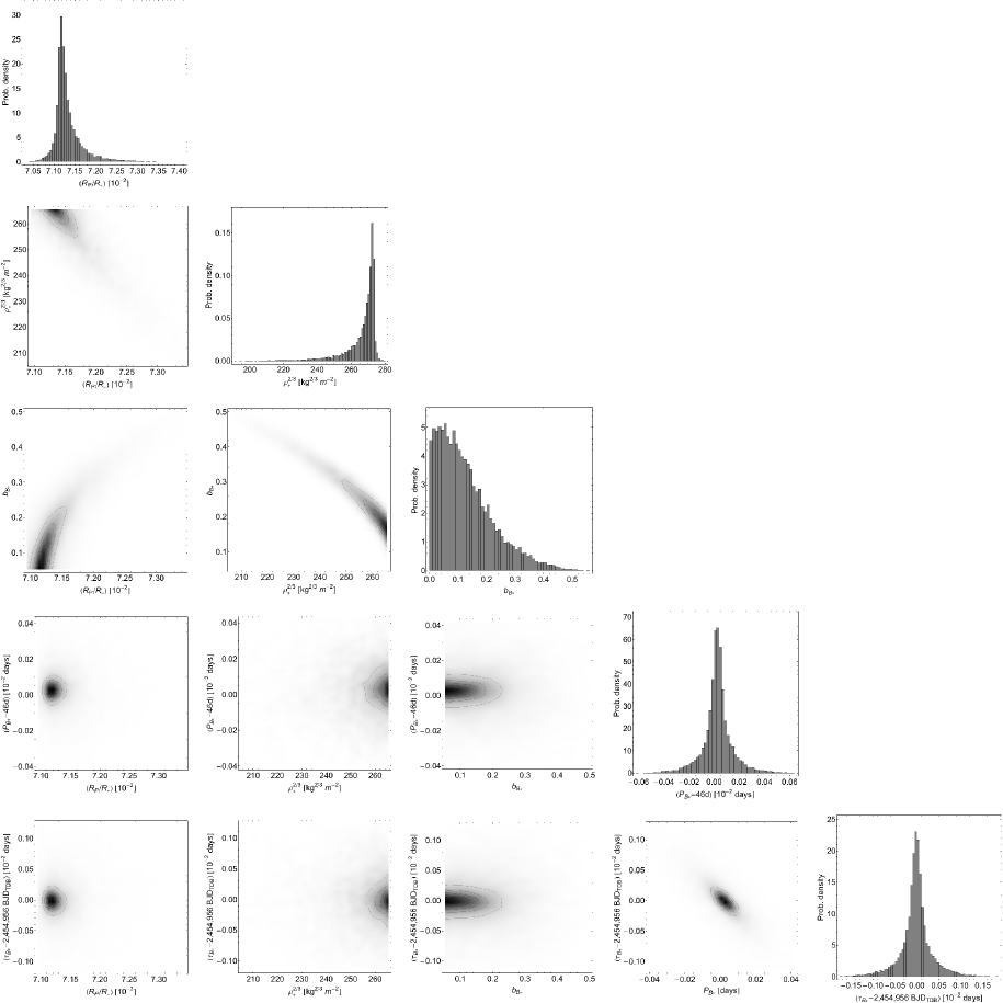
Figure 5.— Marginalised posteriors from MultiNest when fitting a synthetic example of a planet-only data set using a planet-only model from LUNA.

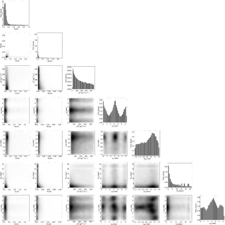
Figure 6.— Marginalised posteriors from MultiNest when fitting a synthetic example of a planet-only data set using a planet-with-moon model from LUNA. We here only show the exomoon-related parameters for brevity.

7.2. Moon Example: HZ Neptune around an M2 star with a Widely Separated Earth-like Moon

As a moon example, we use a synthetic planet-with-moon light curve model from Kipping (2011a). The synthetic data consists of six SC transits of a habitable-zone (HZ) Neptune around an M2-star (as before), observed with Kepler-class photometry (same noise as before). The moon is set to an Earth-mass/radius object at the edge of the Hill sphere on a retrograde orbit. Details of the model can be found in §4.5 of Kipping (2011a) and the de-noised model is shown in the left panel of Figure 2.

Fitting the data using MultiNest with a planet-only model yields a Bayesian evidence of $\log\mathcal{Z}_{0}=22104.55\pm 0.21$, whereas the planet-with-moon model reaps $\log\mathcal{Z}_{1}=23552.75\pm 0.27$. The corresponding posteriors of both models are shown in Figures 7&8. The change in evidence corresponds to a $54$-$\sigma$ detection, which is close to the 50-$\sigma$ detection found using a simple F-test in Kipping (2011a). However, MultiNest reveals that three distinct modes exist in the data, which are reported in Table 2. Modes 1 & 3 correspond the correct exomoon orbital period of $23.995$ d, but mode 2 is located at $P_{SB}=15.775$ d. This corresponds to a harmonic, as originally predicted in Kipping (2009a). This is confirmed by evaluating the expected position of the first harmonic using $[(1/P_{SB})+(1/P_{B*})]^{-1}=15.769$ d.

Modes 1 and 3 both locate the true period and both exhibit a significantly improved evidence value. In fact, mode 2 is disfavoured at the $>$7-$\sigma$ level over modes 1 and 3. Between modes 1 and 3, the difference is that mode 3 occurs at the correct retrograde solution whereas mode 1 is prograde. The evidence difference between these modes is $|\Delta(\log\mathcal{Z})=1.2\pm 0.6$ i.e. insignificant. In a blind analysis, there would be no way of reliably distinguishing the correct solution based upon the available data, but more transits should help since the TDV-TIP effect is asymmetric with respect to the orbital sense of motion.

Despite the presence of three modes, MultiNest provides an appropriately weighted global posterior as well as the local posteriors. Using this weighted posterior heavily deweights mode 2 and the leads to accurate values for the key terms such as mass, radius and density (see last column of Table 2. Orbital angles such as inclination become unconstrained due to mixing the prograde and retrograde solutions together, but this is an accurate representation of our ignorance of this term.

Table 2Comparison of exomoon parameter estimates from three modes found in the MultiNest fits of synthetic data. Data generated for a Neptune with a distant moon around an M2 star. The global evidence of the planet-with-moon model (all three modes) is $\log\mathcal{=}$. Mode 3 is the most accurate mode but the local evidence values between modes 1 and 3 are sufficiently close that distinguishing these modes blindly would not be possible (mode 2, however, can be discounted).

Parameter	Truth	Mode 1	Mode 2	Mode 3	Global
$\log\mathcal{Z}$	-	$23552.49\pm 0.36$	$23523.81\pm 0.99$	$23551.27\pm 0.45$	$23552.75\pm 0.27$
Moon params.
$R_{S}/R_{P}$	$0.2570$	$0.2587_{-0.0069}^{+0.0053}$	$0.2559_{-0.0065}^{+0.0051}$	$0.2587_{-0.0070}^{+0.0052}$	$0.2585_{-0.0069}^{+0.0053}$
$M_{S}/M_{P}$	$0.0583$	$0.0620_{-0.0058}^{+0.0086}$	$0.0672_{-0.0073}^{+0.0072}$	$0.0622_{-0.055}^{+0.0096}$	$0.0624_{-0.0059}^{+0.0092}$
$[\rho_{P}]^{2/3}$ [kg2/3 m-2]	$139.0$	$134.5_{-4.7}^{+5.8}$	$229.4_{-8.9}^{+10.2}$	$134.7_{-4.4}^{+6.6}$	$134.9_{-4.5}^{+11.0}$
$i_{SB}$ [∘]	$267.06$	$90.1_{-1.5}^{+1.4}$	$270.20_{-0.70}^{+1.20}$	$270.1_{-1.2}^{+1.3}$	$90_{-3}^{+180}$
$\Omega_{SB}$ [∘]	$5$	$37_{-72}^{+24}$	$25_{-71}^{+18}$	$16_{-69}^{+24}$	$28_{-73}^{+23}$
$P_{SB}$ [days]	$23.995$	$23.990_{-0.047}^{+0.020}$	$15.755_{-0.014}^{+0.010}$	$23.989_{-0.053}^{+0.019}$	$23.987_{-0.081}^{+0.021}$
$\phi_{SB}$ [∘]	$40$	$173_{-72}^{+25}$	$23_{-18}^{+70}$	$31_{-24}^{+69}$	$112_{-95}^{+75}$

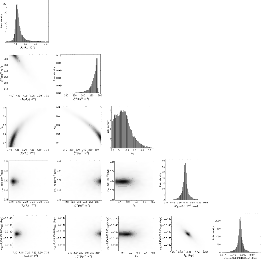
Figure 7.— Marginalised posteriors from MultiNest when fitting a synthetic example of a planet-with-moon data set using a planet-only model from LUNA.

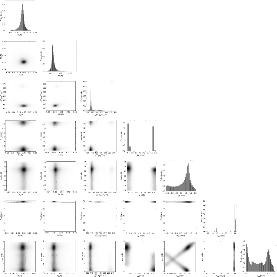
Figure 8.— Marginalised posteriors from MultiNest when fitting a synthetic example of a planet-with-moon data set using a planet-with-moon model from LUNA. We here only show the exomoon-related parameters for brevity.

8. SUMMARY

In this work, we have presented a description of the objectives and methods of our new observational project, “The Hunt for Exomoons with Kepler” (HEK). The HEK project will seek to infer the presence of extrasolar moons around transiting exoplanet candidates observed by the Kepler Mission. In cases of null detections, upper limits will be reported and the full set of parameter posteriors will be made available on the project website (www.cfa.harvard.edu/HEK/). These statistics may be used to deduce the frequency of large moons around viable exoplanet hosts, $\eta_{\leftmoon}$.

We have described, in §4, how the list of all Kepler Objects of Interest (KOIs) will be distilled into a subset of the most promising candidates, for the purposes of exomoon detection, via a three-prong target selection (TS) strategy. This includes visual identification (TSV), automatic filtering (TSA) and targets-of-opportunity (TSO) with a final stage of target prioritization (TSP).

Selected targets will be interrogated for evidence of an exomoon by comparing the Bayesian evidence, $\mathcal{Z}$ of a planet-only model and a planet-with-moon model (see discussion in §5.2). In addition to presenting a $>4$-$\sigma$ preference for the planet-with-moon model, putative candidates must demonstrate physically plausible solutions.

In fitting the data, we require both a forward-model and a fitting algorithm. The former task is handled by the LUNA algorithm, developed by Kipping (2011a), which is designed to analytically model the transit light curve of a planet-with-moon system including limb darkening, dynamical motion and mutual events. Due to the highly complex parameter space, featuring multiple modes due to aliased harmonic power, and the need for an highly efficient computation of the Bayesian evidence, a sophisticated fitting algorithm is required. To this end, we have presented the application of MultiNest (Feroz et al., 2007) with LUNA. MultiNest is a multimodal nested sampling algorithm widely used in the cosmology and particle physics communities. §5.3 describes our implementation and the choice of priors, parameterization and likelihood function.

Strategies for vetting potential candidates are discussed in §6 before we present two examples of LUNA+MultiNest on synthetic data in §7. The example fits demonstrate not only the multimodal nature of looking for exomoons but also how Bayesian evidence may be used to detect such systems.

We are currently analyzing a subset of preferred candidates and will be reporting on these findings in the near-future (Kipping et al. 2012, in prep.). As the HEK project progresses, we hope to answer the question as to whether large moons, possibly even Earth-like habitable moons, are common in the Galaxy or not. Enabled by the exquisite photometry of Kepler, exomoons may soon move from theoretical musings to objects of empricial investigation.

Appendix

Table 3List of important acromyms used in this paper.

Acromyn	Definition
HEK	Hunt for Exomoons with Kepler project
SC	short-cadence
LC	long-cadence
KIC	Kepler Input Catalogue
TTV	Transit timing variations
TDV	Transit duration variations
TDV-V	Velocity induced TDV
TDV-TIP	Transit impact parameter induced TDV
TS	Target selection
TSA	Automatic target selection
TSV	Visual target selection
TSP	Prioritization target selection

Table 4List of important parameters used in this paper.

Parameter	Definition
$S_{B*}$	Sky-projected separation between the planet-moon barycentre and the host star, in units of $R_{*}$
$\nu_{SB}$	True anomaly of the satellite around the planet-moon barycentre
$e_{B*}$	Orbital eccentricity of the barycentre of the planet (+ any satellites) around the host star
$e_{SB}$	Orbital eccentricity of the satellite around the planet-moon barycentre
$\omega_{B*}$	Argument of periapsis of the barycentre of the planet (+ any satellites) around the host star
$\omega_{SB}$	Argument of periapsis of the satellite around the planet-moon barycentre
$i_{B*}$	Orbital inclination of the barycentre of the planet (+ any satellites) around the host star
$i_{SB}$	Orbital inclination of the satellite around the planet-moon barycentre
$\Omega_{SB}$	Longitude of the ascending node of a satellite, relative to the orbital plane of the planet
$R_{*}$	Radius of the host star
$R_{P}$	Radius of the planet
$R_{S}$	Radius of the satellite
$a$	Semi-major axis of an object around its primary
$a_{B*}$	Semi-major axis of the planet-moon barycentre around the host star
$a_{SB}$	Semi-major axis of the satellite around the planet-moon barycentre
$P_{B*}$	Orbital period of the barycentre of the planet (+ any satellites) around the host star
$P_{SB}$	Orbital period of the satellite around the planet-moon barycentre
$M_{*}$	Mass of the star
$M_{P}$	Mass of the planet
$M_{S}$	Mass of the satellite
$\rho_{*}$	Mean density of the star
$\rho_{P}$	Mean density of the planet
$\rho_{S}$	Mean density of the satellite
$p$	Ratio of the planet’s radius to the stellar radius ($R_{P}/R_{*}$)
$s$	Ratio of the satellite’s radius to the stellar radius ($R_{S}/R_{*}$)
$\delta$	Defined as $p^{2}$
$\tau_{B*}$	Instant when $\mathrm{d}S_{B*}/\mathrm{d}t=0$ near inferior conjunction
$b_{B*}$	Impact parameter of the barycentre of the planet (+ any satellites)
$\tilde{T}$	Time between the planet’s centre crossing the stellar limb to exiting under the same condition
$\delta_{\mathrm{TTV}}$	RMS amplitude of TTV signal
$\delta_{\mathrm{TDV-V}}$	RMS amplitude of TDV-V signal
$\delta_{\mathrm{TDV-TIP}}$	RMS amplitude of TDV-TIP signal
$\Lambda_{\mathrm{TTV}}$	Waveform of TTV signal
$\Lambda_{\mathrm{TDV-V}}$	Waveform of TDV-V signal
$\Lambda_{\mathrm{TDV-TIP}}$	Waveform of TDV-TIP signal
$\Phi_{\mathrm{TTV}}$	Enhancement factor of TTV signal
$\Phi_{\mathrm{TDV-V}}$	Enhancement factor of TDV-V signal
$\Phi_{\mathrm{TDV-TIP}}$	Enhancement factor of TDV-TIP signal
$Q_{P}$	Tidal quality factor of the planet
$k_{2p}$	Love number of the planet
$\mathbb{T}$	Lifetime of the moon

References

- Abdussalam et al. (2010) Abdussalam, S. S., Allanach, B. C., Quevedo, F., Feroz, F. & Hobson, M., 2010, Phys. Rev., D81, 035017
- Agnor & Hamilton (2006) Agnor, C. B. & Hamilton, D. P., 2006, Nature, 441, 192
- Agol et al. (2005) Agol, E., Steffen, J., Sari, R. & Clarkson, W., 2005, MNRAS, 359, 567
- Anderson et al. (2010) Anderson, D. R. et al., 2010, ApJ, 709, 159
- Bakos et al. (2009) Bakos, G. A. et al., 2009, ApJ, 710, 1724
- Barnes & O’Brien (2002) Barnes, J. W. & O’Brien, D. P., 2002, ApJ, 575, 1087
- Batalha et al. (2012) Batalha, N. et al., 2012, in prep.
- Borucki et al. (2011) Borucki, W. J. et al., 2011, ApJ, 736, 19
- Ter Braak (2006) Ter Braak, C. J. F., 2006, Stat. Comput. 16, 239
- Brown et al. (2001) Brown, T. M., Charbonneau, D., Gilliland, R. L., Noyes, R. W. & Burrows, A., 2001, ApJ, 552, 699
- Brown et al. (2011) Brown, T. M., Latham, D. W., Everett, M. E. & Esquerdo, G. A., 2011, AJ, 142, 112
- Canup & Ward (2006) Canup, R. M. & Ward, W. R., 2006, Nature, 441, 834
- Carter et al. (2008) Carter, J. A., Yee, J. C., Eastman, J., Gaudi, B. S. & Winn, J. N., 2008, ApJ, 689, 499
- Carter et al. (2009) Carter, J. A., Winn, J. N., Gilliland, R. & Holman, M. J., 2009, ApJ, 696, 241
- Cassidy et al. (2009) Cassidy, T. A., Mendez, R., Arras, P., Johnson, R. E. & Skrutskie, M. F., 2009, ApJ, 704, 1341
- Castelli & Kurucz (2004) Castelli, F. & Kurucz, R. L., 2004, astro-ph:0405087
- Cochran et al. (2011) Cochran, W. D. et al., 2011, ApJS, 197, 7
- Claret (2000) Claret A., 2000, A&A, 363, 1081
- Cox (2000) Cox, A. N. (ed.), Allen’s Astrophysical Quantities (4th edition) (Springer, Heidelberg), 2000.
- D’Angelo et al. (2010) D’Angelo G., Durisen R. H. & Lissauer J. J., 2010, Exoplanets, ed. S. Seager, University of Arizona Press, p. 319
- Deeg (2009) Deeg, H. 2009, IAU Symp., 253, 388
- Deleuil et al. (2008) Deleuil, M. et al., 2008, A&A, 491, 889
- Deming et al. (2011) Deming, D. et al., 2011, ApJ, 740, 33
- Domingos et al. (2006) Domingos, R. C., Winter, O. C. & Yokoyama, T., 2006, MNRAS, 373, 1227
- Eberle et al. (2010) Eberle, J. Cuntz, M., Quarles, B. & Musielak, Z. E., 2011, Int. Jour. Astrobiology, 10, 325
- Elser et al. (2011) Elser, S., Moore, B., Stadel, J. & Morishima, R., 2011, Icarus, 214, 357
- Feroz et al. (2007) Feroz, F. & Hobson, M. P., 2007, MNRAS, 384, 449
- Feroz et al. (2009a) Feroz, F., Hobson, M. P. & Bridges, M., 2009a, MNRAS, 398, 1601
- Feroz et al. (2009b) Feroz, F., Gair, J. R., Hobson, M. P. & Porter, E. K., 2009b, CQG, 26, 215003
- Feroz et al. (2011) Feroz, F., Balan, S. T. & Hobson, M. P., 2011, MNRAS, 416, L104
- Fewell (2006) Fewell, M., “Area of Common Overlap of Three Circles”, Tech. Rep. DSTO-TN-0722, 2006. [Online]. Available: http://hdl.handle.net/1947/4551
- Fischer et al. (2012) Fischer, D. A. et al., 2012, MNRAS, 419, 2900
- Ford & Holman (2007) Ford, E. B. & Holman, M. J., 2007, ApJ, 664, 51
- Fossey et al. (2012) Fossey, S. J., Kipping, D. M. et al., 2012, in prep.
- Geyer (1991) Geyer, C. J., 1991, in “Computing Science and Statistics: 23rd symposium on the interface”, American Statistical Association, New York, p. 156
- Gillon et al. (2011) Gillon, M. et al., 2012, A&A, 539, 28
- Girardi et al. (2000) Girardi, L., Bressan, A., Bertelli, G., & Chiosi, C., 2000, A&AS, 141, 371
- Goldreich & Soter (1966) Goldreich, P. & Soter, S. 1966, Icarus, 5, 375
- Gregory (2009) Gregory, P. C., 2009, in “Bayesian Inference and Maximum Entropy Methods in Science and Engineering: 27th International Workshop”, Saratoga Springs, eds. K. H. Knuth, A. Caticha, J. L. Center, A,G ̵̇ iffin, C. C. Rodrguez, AIP Conference Proceedings, 954, 307
- Heller et al. (2011) Heller, R. Leconte, J. & Barnes, R., 2011, A&A, 528, 27
- Henry et al. (2011) Henry, G. W., Howard, A. W., Marcy, G. W., Fischer, D. A. & Johnson, J. A., 2011, ApJ, submitted (astro-ph:1109.2549)
- Holman & Murray (2005) Holman, M. J. & Murray, N. W., 2005, Science, 307, 1288
- Hubbard (1984) Hubard W. B., 1984, Planetary Interiors (New York: Van Nostrand Reinhold)
- Kipping (2009a) Kipping, D. M., 2009a, MNRAS, 392, 181
- Kipping (2009b) Kipping, D. M., 2009b, MNRAS, 396, 1797
- Kipping et al. (2009) Kipping, D. M., Fossey, S. J. & Campanella, G., 2009, MNRAS, 400, 398
- Kipping (2010a) Kipping, D. M., 2010a, MNRAS, 407, 301
- Kipping (2010b) Kipping, D. M., 2010b, MNRAS, 408, 1758
- Kipping (2010c) Kipping, D. M., 2010c, MNRAS, 409, L119
- Kipping & Bakos (2011a) Kipping, D. M. & Bakos, G. A., 2011a, ApJ, 730, 50
- Kipping & Bakos (2011b) Kipping, D. M. & Bakos, G. A., 2011b, ApJ, 733, 36
- Kipping & Tinetti (2010) Kipping, D. M. & Tinetti, G., 2010, MNRAS, 407, 2589
- Kipping (2011a) Kipping, D. M., 2011a, MNRAS, 416, 689
- Kipping (2011b) Kipping, D. M., 2011b, PhD thesis, University College London (astro-ph:1105.3189)
- Kipping et al. (2012) Kipping, D. M., Dunn, W., Jasinski, J. & Manthri, V. M., 2012, MNRAS, accepted (astro-ph:1112.2700)
- Kundurthy et al. (2011) Kundurthy, P., Agol, E., Becker, A. C., Barnes, R., Williams, B & Mukadam, A., 2011, ApJ, 731, 123
- Lewis (2011) Lewis, K. M. 2011, PhD thesis, Monash Univ., Australia (astro-ph:1109.5332)
- Liddle et al. (2007) Liddle, A. R., 2007, MNRAS, 377, L74
- Lintott et al. (2012) Lintott, C. et al., 2012, AJ, submitted (astro-ph:1202.6007)
- Mandel & Agol (2002) Mandel, K. & Agol, E., 2002, ApJ, 580, 171
- Mislis et al. (2011) Mislis, D., Heller, R., Schmitt, J. H. M. M. & Hodgkin, S. 2011, astro-ph:1112.2008
- Muirhead et al. (2011) Muirhead, P., Hamren, K., Schlawin, E., Rojas-Ayala, B., Covey, K. R. & Lloyd, J. P., 2011, ApJL, submitted (astro-ph:1109.1819)
- Mukherjee et al. (2006) Mukherjee P., Parkinson D. & Liddle A. R., 2006, ApJ, 638, L51
- Namouni (2010) Namouni, F., 2010, ApJ, 719, 145
- Nesvorný & Beaugé (2010) Nesvorný, D. & Beaugé, C., 2010, ApJ, 709, 44
- Ó Ruanaidh & Fitzgerald (2011) Ó Ruanaidh J. & Fitzgerald W., 1996, Numerical Bayesian Methods Applied to Signal Processing. Springer Verlag:New York
- Pál (2011) Pál, A., 2011, MNRAS, 420, 1630
- Podsiadlowski et al. (2010) Podsiadlowski, P., Rappaport, S., Fregeau, J. M. & Mardling, R. A., 2010, ApJ, submitted (astro-ph:1007.1418)
- Porter & Grundy (2011) Porter, S. B. & Grundy, W. M., 2011, ApJ, 736, 14
- Ragozzine & Holman (2010) Ragozzine, D. & Holman, M. J., 2010, astro-ph:1006.3727
- Sanchis-Ojeda & Winn (2011) Sanchis-Ojeda, R. & Winn, J. N., 2011, ApJ, 743, 61
- Sartoretti & Schneider (1999) Sartoretti, P. & Schneider, J., 1999, A&AS, 14, 550
- Sato & Asada (2009) Sato, M. & Asada, H., 2009, PASJ, 61, 29
- Seager & Mallén-Ornelas (2003) Seager, S., & Mallén-Ornelas, G., 2003, ApJ, 585, 1038
- Simon et al. (2009) Simon, A. E., Szabó, Gy. M. & Szatmáry, K., 2009, EM&P, 105, 385
- Skilling (2004) Skilling, J. 2004, in Fischer R., Preuss R., Toussaint U. V., eds, American Institute of Physics Conference Series Nested Sampling. pp 395–405
- Szabó et al. (2006) Szabó, Gy. M., Szatmáry, K., Divéki, Zs. & Simon, A., 2006, A&A, 2006, 450, 395
- Taylor (1992) Taylor, S. R., 1992, “Solar system evolution: a new perspective. an inquiry into the chemical composition, origin, and evolution of the solar system”, Cambridge University Press, Cambridge, UK
- Torres et al. (2004) Torres, G. Konacki, M., Sasselov, D. D. & Jha, S., 2004, ApJ, 614, 979
- Torres (2007) Torres, G. et al., 2007, ApJ, 671, 65
- Torres et al. (2011) Torres, G. et al., 2011, ApJ, 727, 24
- Tusnski & Valio (2011) Tusnski, L. R. M. & Valio, A., 2011, ApJ, 743, 97
- Valencia et al. (2006) Valencia, D., Sasselov, D. D. & O’Connell, R. J., 2006, Icarus, 181, 545
- Vegetti et al. (2010) Vegetti, S., Koopmans, L. V. E., Bolton, A., Treu, T. & Gavazzi, R., 2010, MNRAS, 408, 1969
- Williams et al. (1997) Williams, D. M., Kasting, J. F. & Wade, R. A., 1997, Nature, 385, 234
- Williams et al. (2011) Williams, D. M., 2011, Oral Presentation, Kepler Science Conference, NASA Ames, California