Band-gaps in electrostatically controlled dielectric laminates subjected to incremental shear motions

Abstract.

The thickness vibrations of a finitely deformed infinite periodic laminate made out of two layers of dielectric elastomers is studied. The laminate is pre-stretched by inducing a bias electric field perpendicular the the layers. Incremental time-harmonic fields superimposed on the initial finite deformation are considered next. Utilizing the Bloch-Floquet theorem along with the transfer matrix method we determine the dispersion relation which relates the incremental fields frequency and the phase velocity.

Ranges of frequencies at which waves cannot propagate are identified whenever the Bloch-parameter is complex. These band-gaps depend on the phases properties, their volume fraction, and most importantly on the electric bias field. Our analysis reveals how these band-gaps can be shifted and their width can be modified by changing the bias electric field. This implies that by controlling the electrostatic bias field desired frequencies can be filtered out. Representative examples of laminates with different combinations of commercially available dielectric elastomers are examined.

Keywords: dielectric elastomers; wave propagation; finite deformations; thickness vibrations; non-linear electroelasticity, band-gap, composite, Bloch-Floquet analysis.

^†Department of Mechanical Engineering

Ben-Gurion University

Beer-Sheva, 84105

Israel

^‡Department of Biomedical Engineering

Ben-Gurion University

Beer-Sheva, 84105

Israel

1. Introduction

Band-gaps corresponding to ranges of frequencies at which waves cannot propagate earned the interest of the scientific community (e.g., Ziegler, 1977; Wang and Auld, 1985; Kushwaha et al., 1994; Gei et al., 2004, 2009, to name a few). These band-gaps (BGs) or stop-bands can be utilized for various applications such as filtering elastic waves, enhancing performance of ultrasonic transducers, supplying a vibrationless ambient when needed for industrial and biomedical applications, and more. Several techniques are available for investigating wave propagation in composites, (e.g., for the plane-wave method in periodic composites Kushwaha et al., 1993; Tanaka and Tamura, 1998; Sigalas and Economou, 1996) and the effective medium methods (e.g., Sabina and Willis, 1988, for composites with random microstructre). As in this work we are interested in the appearance of BGs in infinite periodic laminates, we find it convenient to use the transfer matrix method (Wang and Auld, 1986), along with the Bloch-Floquet theorem (Kohn et al., 1972). Specifically, we consider waves superposed on a pre-deformed state due to bias electric field acting on an infinite periodic laminate with a repeating sequence of of dielectric elastomers (DEs) layers. The motivation for the choice of DEs as the composite constituents stems from their ability to undergo large deformations (Pelrine et al., 2000), and to change their mechanical and dielectric properties when subjected to electrostatic fields (Kofod, 2008), thus effecting the way in which electroelastic waves propagate in the matter (Shmuel et al., 2011; Gei et al., 2011). As will be shown in the sequel, by properly tuning the bias electrostatic field different ranges of frequencies can be filtered out.

The structure of this paper is as follows. Following the works of Dorfmann and Ogden (2005); deBotton et al. (2007); Dorfmann and Ogden (2010); Bertoldi and Gei (2011); Rudykh and deBotton (2011); Ponte Castañeda and Siboni (2011) and Tian et al. (2012), the background required for describing the static and dynamic responses of elastic dielectric laminates is revisited in section 2. Particularly, the governing equations for small fields superimposed on large deformations of electroactive elastomers are summarized. In this section we also introduce an adequate extension of the transfer matrix method and the Bloch-Floquet theorem required for treating the propagation of incremental electroelastic waves superimposed on finitely deformed DE laminates. Section 3 deals with the response an infinite periodic laminate with alternating layers, whose behaviors are governed by the incompressible dielectric neo-Hookean model (DH), to a fixed electric displacement field normal to the layers plane. Subsequently, the response to small harmonic perturbations superimposed on the finitely deformed laminate is analyzed. The end result is given in terms of a dispersion relation relating the incremental fields frequency and phase velocity to the Bloch-parameter. Several examples are considered in section 4, where the influence of the morphology of the laminate, the contrast between the phases properties, and the bias electric field on the dispersion relation is examined. Finally, realizable tunable isolators are studied by considering combinations of commercially available DEs such as VHB 4910, fluorosilicone 730 and ELASTOSIL RT-625.

2. Theoretical background

Consider a heterogeneous body occupying a volume region $\Omega_{0}\subset\mathbb{R}^{3}$ made out of $N$ perfectly bonded different homogeneous phases. The external boundary of the body $\partial\Omega_{0}$ separates it from the surrounding space $\mathbb{R}^{3}\backslash\Omega_{0}$, assumed to be vacuum. Each phase occupies a volume region $\Omega_{0}^{\left(r\right)}\left(r=1,2,...,N\right)$ and its boundary is $\partial\Omega_{0}^{\left(r\right)}$. Let $\boldsymbol{\chi}:\Omega_{0}\times\mathcal{I}\rightarrow\mathbb{R}^{3}$ describe a continuous and twice-differentiable mapping of a material point $\mathbf{X}$ from the reference configuration of the body to its current configuration $\Omega$ with boundary $\partial\Omega$ by $\mathbf{x}=\boldsymbol{\chi}\left(\mathbf{X},t\right)$. The corresponding velocity and acceleration are denoted, respectively, by $\mathbf{v}=\boldsymbol{\chi}_{,t}$ and $\mathbf{a}=\boldsymbol{\chi}_{,tt},$ and the deformation gradient is $\mathbf{F}=\nabla_{\mathbf{X}}\boldsymbol{\chi}.$ Vectors in the neighborhood of $\mathbf{X}$ are transformed into vectors in the current configuration via $\mathrm{d}\mathbf{x}=\mathbf{F}\mathrm{d}\mathbf{X}$. The volume change of a referential volume element $\mathrm{d}V$ is given by $\mathrm{d}v=J\mathrm{d}V$, where $\mathrm{d}v$ is the corresponding volume element in the current configuration, and $J\equiv\det\left(\mathbf{F}\right)>0$ due to material impenetrability. The conservation of mass implies that $\rho_{L}=J\rho$, where $\rho_{L}$ and $\rho$ are the material mass densities in the reference and the deformed configurations, respectively. An area element $\mathrm{d}A$ with the unit normal $\mathbf{N}$ in the reference configuration is transformed to a deformed area $\mathrm{d}a$ with the unit normal $\mathbf{n}$ in the current configuration according to Nanson’s formula $\mathbf{N}\mathrm{d}A=\frac{1}{J}\mathbf{F}^{\mathrm{T}}\mathbf{n}\mathrm{d}a$. The right and left Cauchy-Green strain tensors are $\mathbf{C}=\mathbf{F}^{\mathrm{T}}\mathbf{F}$ and $\mathbf{b}=\mathbf{F}\mathbf{F}^{\mathrm{T}}$.

The electric field in the current configuration, denoted by $\mathbf{e}$, is given in terms of a gradient of a scalar field, termed the electrostatic potential. In free space an induced electric displacement field $\mathbf{d}$ is related to the electric field via the vacuum permittivity $\epsilon_{0}$, such that $\mathbf{d}=\epsilon_{0}\mathbf{e}$. In dielectric bodies the connection between the fields is specified by an adequate constitutive relation.

In terms of a ’total’ stress tensor $\boldsymbol{\sigma}$ the equations of motion read

$$\nabla\cdot\boldsymbol{\sigma}=\rho\mathbf{a},$$ (1)

where in order to satisfy the balance of angular momentum symmetry of $\boldsymbol{\sigma}$ is required. The terminology ’total’ stress is used to indicate that $\boldsymbol{\sigma}$ accounts for both mechanical and electrical contributions. Thus, the traction $\mathbf{t}$ on a deformed area element with a unit normal $\mathbf{n}$ is given by

$$\boldsymbol{\sigma}\mathbf{n}=\mathbf{t}.$$ (2)

When ideal dielectrics are considered no free body charge is present, and Gauss’s law takes the form

$$\nabla\cdot\mathbf{d}=0.$$ (3)

Faraday’s law is

$$\nabla\times\mathbf{e}=\mathbf{0},$$ (4)

when a quasi-electrostatic approximation is considered. A full description of the system should consider interactions with fields outside the body, henceforth denoted by a star superscript. Specifically, these are

$$\mathbf{d}^{\star} = \epsilon_{0}\mathbf{e}^{\star},$$ (5)

$$\boldsymbol{\sigma}^{\star} = \epsilon_{0}\left[\mathbf{e}^{\star}\otimes\mathbf{e}^{\star}-\frac{1}{2}\left(\mathbf{e}^{\star}\cdot\mathbf{e}^{\star}\right)\mathbf{I}\right],$$ (6)

where $\mathbf{I}$ is the identity tensor. In vacuum the governing Eqs. (3)-(4) for $\mathbf{d}^{\star}$ and $\mathbf{e}^{\star}$ are equivalent to Laplace’s equation for the electrostatic potential. As a consequence, $\boldsymbol{\sigma}^{\star}$ known as the Maxwell stress, is divergence-free. Across the outer boundary $\partial\Omega$, the electric jump conditions are

$$\left(\mathbf{d}-\mathbf{d}^{\star}\right)\cdot\mathbf{n}=-w_{e}, \left(\mathbf{e}-\mathbf{e}^{\star}\right)\times\mathbf{n}=\mathbf{0},$$ (7)

where $w_{e}$ is the surface charge density. In order to formulate the jump in the stress we postulate a separation of the traction into a sum of a prescribed mechanical traction $\mathbf{t}_{m}$, and an electric traction $\mathbf{t}_{e}$ induced by the external stress such that $\mathbf{t}_{e}=\boldsymbol{\sigma}^{\star}\mathbf{n}$. Hence, the stress boundary condition is

$$\left(\boldsymbol{\sigma}-\boldsymbol{\sigma}^{\star}\right)\mathbf{n}=\mathbf{t}_{m}.$$ (8)

The jump conditions across a charge-free internal boundary between two adjacent phases $m$ and $f$ are

$$\left[\left[\boldsymbol{\sigma}\right]\right]\mathbf{n}=\mathbf{0}, \left[\left[\mathbf{d}\right]\right]\cdot\mathbf{n}=0, \left[\left[\mathbf{e}\right]\right]\times\mathbf{n}=\mathbf{0},$$ (9)

where $\left[\left[\bullet\right]\right]\equiv\left(\bullet\right)^{\left(b\right)}-\left(\bullet\right)^{\left(a\right)}$ denotes the jump of fields between the two phases.

A Lagrangian formulation of the governing equations and jump conditions is feasible by a pull-back of the Eulerian fields

$$\mathbf{P}=J\boldsymbol{\sigma}\mathbf{F}^{\mathrm{-T}}, \mathbf{D}=J\mathbf{F}^{-1}\mathbf{d}, \mathbf{E}=\mathbf{F}^{\mathrm{T}}\mathbf{e},$$ (10)

for the ’total’ first Piola-Kirchhoff stress, Lagrangian electric displacement and electric field, respectively. Thus, the governing Eqs. (1), (3) and (4) transform, respectively, to

$$\nabla_{\mathbf{X}}\cdot\mathbf{P}=\rho_{L}\mathbf{a}, \nabla_{\mathbf{X}}\cdot\mathbf{D}=0, \nabla_{\mathbf{X}}\times\mathbf{E}=\mathbf{0}.$$ (11)

The corresponding referential jump conditions across the external boundary $\partial\Omega_{0}$ are

$$\left(\mathbf{P}-\mathbf{P}^{\star}\right)\mathbf{N}=\mathbf{t}_{M}, \left(\mathbf{D}-\mathbf{D}^{\star}\right)\cdot\mathbf{N}=-w_{E}, \left(\mathbf{E}-\mathbf{E}^{\star}\right)\times\mathbf{N}=\mathbf{0},$$ (12)

where $\mathbf{t}_{M}\mathrm{d}A=\mathbf{t}_{m}\mathrm{d}a$ and $w_{E}\mathrm{d}A=w_{e}\mathrm{d}a$. Across the referential interfaces Eqs. (9) become

$$\left[\left[\mathbf{P}\right]\right]\mathbf{N}=0, \quad\left[\left[\mathbf{D}\right]\right]\cdot\mathbf{N}=0, \quad\left[\left[\mathbf{E}\right]\right]\times\mathbf{N}=\mathbf{0}.$$ (13)

Following Dorfmann and Ogden (2005), the constitutive relation is expressed in terms of an augmented energy density function (AEDF) $\Psi$ with the independent variables $\mathbf{F}$ and $\mathbf{D}$, such that the total first Piola-Kirchhoff stress and the Lagrangian electric field are derived via

$$\mathbf{P}=\frac{\partial\Psi}{\partial\mathbf{F}},\quad\mathbf{E}=\frac{\partial\Psi}{\partial\mathbf{D}}.$$ (14)

The first of Eq. (14) should be modified when considering incompressible materials, as the kinematic constraint yields an additional workless part of stress. The latter is accounted by introducing a Lagrange multiplier $p_{0}$ which can determined only from the equilibrium equations together with the boundary conditions. Thus, the total first Piola-Kirchhoff is

$$\mathbf{P}=\frac{\partial\Psi}{\partial\mathbf{F}}-p_{0}\mathbf{F}^{\mathrm{-T}}.$$ (15)

Based on the framework developed in Dorfmann and Ogden (2010), we superimpose an infinitesimal time-dependent elastic and electric displacements $\dot{\mathbf{x}}=\dot{\boldsymbol{\chi}}\left(\mathbf{X},t\right)$ and $\dot{\mathbf{D}}\left(\mathbf{X},t\right)$, on the pre-deformed configuration. Herein, and in the sequel, we use a superposed dot to denote incremental quantities. Let the Eulerian quantities $\boldsymbol{\Sigma},\check{\mathbf{d}},\ \mathrm{and}\ \check{\mathbf{e}}$ denote the push-forwards of increments in the first Piola-Kirchhoff stress, the Lagrangian electric displacement and electric fields, respectively, namely

$$\boldsymbol{\Sigma}=\frac{1}{J}\dot{\mathbf{P}}\mathbf{F}^{T},\quad\check{\mathbf{d}}=\frac{1}{J}\mathbf{F}\dot{\mathbf{D}},\quad\check{\mathbf{e}}=\mathbf{F}^{-T}\dot{\mathbf{E}}.$$ (16)

In terms of these variables, the incremental governing equations read

$$\nabla\cdot\boldsymbol{\Sigma}=\rho\dot{\mathbf{x}}_{,tt}, \quad\nabla\cdot\check{\mathbf{d}}=0, \quad\nabla\times\check{\mathbf{e}}=0.$$ (17)

For an incompressible material the incremental constraint is

$$\nabla\cdot\dot{\mathbf{x}}\equiv\mathrm{tr}\left(\mathbf{h}\right)=0,$$ (18)

where $\mathbf{h}=\nabla\dot{\mathbf{x}}$ is the displacement gradient. Linearization of the incompressible material constitutive equations in the increments yields

$$\boldsymbol{\Sigma} = \boldsymbol{\mathcal{C}}\mathbf{h}+p_{0}\mathbf{h}^{\mathrm{T}}-\dot{p}_{0}\mathbf{I}+\boldsymbol{\mathcal{B}}\check{\mathbf{d}},$$ (19)

$$\check{\mathbf{e}} = \boldsymbol{\mathcal{B}}^{\mathrm{T}}\mathbf{h}+\boldsymbol{\mathcal{A}}\check{\mathbf{d}},$$ (20)

where $\left(\boldsymbol{\mathcal{B}}^{\mathrm{T}}\mathbf{h}\right)_{k}=\mathcal{B}_{ijk}h_{ij}$. The quantities $\boldsymbol{\mathcal{A}},\boldsymbol{\mathcal{B}}$ and $\boldsymbol{\mathcal{C}}$ are the push-forwards of the referential reciprocal dielectric tensor, electroelastic coupling tensor, and elasticity tensor, respectively. In components form

$$\mathcal{A}_{ij}=JF_{\alpha i}^{-1}\mathcal{A}_{0\alpha\beta}F_{\beta j}^{-1}, \mathcal{B}_{ijk}=F_{j\alpha}\mathcal{B}_{0i\alpha\beta}F_{\beta k}^{-1}, \mathcal{C}_{ijkl}=\frac{1}{J}F_{j\alpha}\mathcal{C}_{0i\alpha k\beta}F_{l\beta},$$ (21)

where

$$\mathcal{A}_{0\alpha\beta}=\frac{\partial^{2}\Psi}{\partial D_{\alpha}\partial D_{\beta}},\quad\mathcal{B}_{0i\alpha\beta}=\frac{\partial^{2}\Psi}{\partial F_{i\alpha}\partial D_{\beta}},\quad\mathcal{C}_{0i\alpha k\beta}=\frac{\partial^{2}\Psi}{\partial F_{i\alpha}\partial F_{k\beta}}.$$ (22)

The incremental outer fields are given by

$$\dot{\mathbf{d}^{\star}} = \epsilon_{0}\dot{\mathbf{e}^{\star}},$$ (23)

$$\dot{\boldsymbol{\sigma}^{\star}} = \epsilon_{0}\left[\dot{\mathbf{e}^{\star}}\otimes\mathbf{e}^{\star}+\mathbf{e}^{\star}\otimes\dot{\mathbf{e}^{\star}}-\left(\mathbf{e}^{\star}\cdot\dot{\mathbf{e}^{\star}}\right)\mathbf{I}\right].$$ (24)

Here again $\dot{\mathbf{d}^{\star}}$ and $\dot{\mathbf{e}^{\star}}$ are to satisfy Eqs. (3)-(4), where subsequently $\nabla\cdot\dot{\boldsymbol{\sigma}^{\star}}=\mathbf{0}$.

The push-forward of the increments of Eqs. (12) gives the following incremental jump conditions across the external boundary in the current configuration

$$\left[\boldsymbol{\Sigma}-\dot{\boldsymbol{\sigma}^{\star}}+\boldsymbol{\sigma}^{\star}\mathbf{h}^{\mathrm{T}}-\left(\nabla\cdot\dot{\mathbf{x}}\right)\boldsymbol{\sigma}^{\star}\right]\mathbf{n} = \check{\mathbf{t}}_{m},$$ (25)

$$\left[\check{\mathbf{d}}-\dot{\mathbf{d}^{\star}}-\left(\nabla\cdot\dot{\mathbf{x}}\right)\mathbf{d}^{\star}+\mathbf{h}\mathbf{d}^{\star}\right]\cdot\mathbf{n} = -\check{w}_{e},$$ (26)

$$\left[\mathrm{\check{\mathbf{e}}}-\dot{\mathbf{e}^{\star}}-\mathbf{h}^{\mathrm{T}}\mathbf{e}^{\star}\right]\times\mathbf{n} = \mathbf{0},$$ (27)

where $\check{\mathbf{t}}_{m}\mathrm{d}a=\dot{\mathbf{t}}_{M}\mathrm{d}A$ and $\check{w}_{e}\mathrm{d}a=\dot{w}_{E}\mathrm{d}A$. Similarly, the push forward of the increments of Eqs. (13) results in the following jumps across the internal boundaries

$$\left[\left[\boldsymbol{\Sigma}\right]\right]\mathbf{n}=\mathbf{0}, \left[\left[\check{\mathbf{d}}\right]\right]\cdot\mathbf{n}=0 \left[\left[\mathrm{\check{\mathbf{e}}}\right]\right]\times\mathbf{n}=\mathbf{0}.$$ (28)

Several techniques are available in the literature for tackling the problem of wave propagation in periodic composites. In layered structures it is convenient to utilize the transfer-matrix method in conjunction with the Bloch-Floquet theorem (Adler, 1990). Herein we formulate an adequate adjustment for treating the propagation of incremental electroelastic waves superimposed on a finitely deformed multiphase DE laminates.

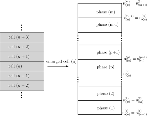
Figure 1. An illustration of an infinite laminate composed of periodic $m$-layers unit-cells.

Consider a finitely deformed infinite DE-laminate made out of $m$-phase periodic unit-cells subjected to incremental perturbations harmonic in time and normal to the layers plane. A schematic illustration of the laminate is shown in Fig. 1. Let $\mathbf{s}_{n}^{\left(p\right)}$, $p=1,..,m$, denote an incremental state vector in the $p$-phase of the $n^{th}$ cell consisting quantities which are continuous across the interface between the two adjacent layers. In view of the linearity of the incremental problem it can be shown that the state vector at the top of the $p$-phase $\mathbf{s}_{t(n)}^{\left(p\right)}$ and the state vector at the bottom of the $p$-phase $\mathbf{s}_{b(n)}^{\left(p\right)}$ (see Fig. 1) are related via a unique non-singular transfer matrix $\mathbf{T}^{\left(p\right)}$ such that

$$\mathbf{s}_{t(n)}^{\left(p\right)}=\mathbf{T}^{\left(p\right)}\mathbf{s}_{b(n)}^{\left(p\right)}.$$ (29)

In terms of the state vectors, the continuity conditions across the interface are

$$\mathbf{s}_{t(n)}^{\left(p\right)}=\mathbf{s}_{b(n)}^{\left(p+1\right)}.$$ (30)

Utilizing Eqs. (29)-(30) recursively the relation between $\mathbf{s}_{t}^{\left(m\right)}$ and $\mathbf{s}_{b}^{\left(1\right)}$ is

$$\mathbf{s}_{t(n)}^{\left(b\right)}=\mathbf{T}^{\left(b\right)}\mathbf{s}_{b(n)}^{\left(b\right)}=\mathbf{T}^{\left(b\right)}\mathbf{s}_{t(n)}^{\left(m-1\right)}=\mathbf{T}^{\left(b\right)}\mathbf{T}^{\left(m-1\right)}\mathbf{s}_{b(n)}^{\left(m-1\right)}=...=\mathbf{T}\mathbf{s}_{b}^{\left(1\right)},$$ (31)

where $\mathbf{T}\equiv\prod_{p=1}^{m}\mathbf{T}^{\left(p\right)}$ is the total transfer matrix.

At one hand the continuity conditions across the interface between two successive cells $n$ and $n+1$ are

$$\mathbf{s}_{b\left(n+1\right)}^{\left(1\right)}=\mathbf{s}_{tn}^{\left(m\right)}.$$ (32)

At the other, the Bloch-Floquet’s theorem states that the state-vectors of the same phase in adjacent cells are identical up to a phase shift in the form

$$\mathbf{s}_{b\left(n+1\right)}^{\left(p\right)}=e^{-ik_{B}h}\mathbf{s}_{b\left(n\right)}^{\left(p\right)},$$ (33)

where $0\leq k_{B}<\pi/h$ is the Bloch-Floquet wavenumber in first irreducible Brillouin zone, representing the smallest region where wave propagation is unique (Kittel, 2005). Substitution of Eq. (31) in (32), followed by employing the latter with Eq. (33), yields the eigenvalue problem

$$\det\left|\mathrm{T}-e^{-ik_{B}h}\mathrm{I}\right|=0,$$ (34)

where $\mathrm{I}$ is an identity matrix with the dimension of the total transfer matrix. The solution of Eq. (34) provides the dispersion relation describing the manner by which waves propagate in the laminate.

3. Thickness vibrations of an infinite periodic two-phase dielectric laminate

Henceforth we restrict our attention to isotropic phases. Consequently, the phases AEDFs can be written in terms of the six invariants (Dorfmann and Ogden, 2005)

$$I_{1}=\mathrm{tr}\left(\mathbf{C}\right)=\mathbf{C}:\mathbf{I}, I_{2}=\frac{1}{2}\left(I_{1}^{2}-\mathbf{C}:\mathbf{C}\right), I_{3}=\det\left(\mathbf{C}\right)=J^{2},$$ (35)

$$I_{4e}=\mathbf{D}\cdot\mathbf{D}, I_{5e}=\mathbf{D}\cdot\mathbf{C}\mathbf{D}, I_{6e}=\mathbf{D}\cdot\mathbf{C}^{2}\mathbf{D}.$$ (36)

Specifically, we consider phases which are characterized by incompressible dielectric neo-Hookean (DH) model

$$\Psi_{DH}^{\left(p\right)}\left(I_{1},I_{5e}\right)=\frac{\mu^{\left(p\right)}}{2}\left(I_{1}-3\right)+\frac{1}{2\epsilon^{\left(p\right)}}I_{5e},$$ (37)

where $\mu^{\left(p\right)}$ and $\epsilon^{\left(p\right)}=\epsilon_{0}\epsilon_{r}^{\left(p\right)}$ denote the phases shear moduli and dielectric constants, respectively, and $\epsilon_{r}^{\left(p\right)}$ being the phases relative dielectric constant. The corresponding total stress is

$$\boldsymbol{\sigma}^{\left(p\right)}=\mu^{\left(p\right)}\mathbf{b}+\frac{1}{\epsilon^{\left(p\right)}}\mathbf{d}\otimes\mathbf{d}-p_{0}^{\left(p\right)}\mathbf{I},$$ (38)

and the current displacement and electric field are related via the isotropic linear relation

$$\mathbf{d}=\epsilon^{\left(p\right)}\mathbf{e}.$$ (39)

Calculation of the associated constitutive tensors $\boldsymbol{\mathcal{A}}^{\left(p\right)},\boldsymbol{\mathcal{B}}^{\left(p\right)},\ \mathrm{and\ }\boldsymbol{\mathcal{C}}^{\left(p\right)}$ yields, in components form,

$$\mathcal{A}_{ij}^{\left(p\right)}=\frac{1}{\epsilon^{\left(p\right)}}\delta_{ij},\quad\mathcal{B}_{ijk}^{\left(p\right)}=\frac{1}{\epsilon^{\left(p\right)}}\left(\delta_{ik}d_{j}+\frac{d_{i}}{\epsilon^{\left(p\right)}}\delta_{jk}\right),\quad\mathcal{C}_{ijkl}^{\left(p\right)}=\mu^{\left(p\right)}\delta_{ik}b_{jl}+\frac{1}{\epsilon^{\left(p\right)}}\delta_{ik}d_{j}d_{l},$$ (40)

where $\delta_{ij}$ are the components of the Kronecker delta.

Consider a Cartesian coordinate system with unit vectors $\mathbf{i_{1},i_{2}}$ and $\mathbf{i_{3}}$ along $x_{1},x_{2}$ and $x_{3}$, respectively. Let a DE laminate be composed of periodic two-phase unit-cells with thickness $H$ along the the $x_{2}$ direction, infinite along the $x_{1}$ and $x_{3}$ directions as illustrated in Fig. 2. For convenience we denote the phases $a$ and $b$. The sum of the phases thicknesses equals the unit-cell thickness $H=H^{\left(a\right)}+H^{\left(b\right)}$, such that $v^{\left(a\right)}=H^{\left(a\right)}/H$ and $v^{\left(b\right)}=H^{\left(b\right)}/H$ are the volume fractions of phase $a$ and phase $b$, respectively. We assume that the composite is allowed to expand freely in the $x_{1}$ and $x_{3}$ directions. Of interest is the composite response when subjected to an overall electric displacement field $\bar{\mathbf{d}}=d_{2}\mathbf{i_{2}}$, where $d_{2}\equiv v^{\left(a\right)}d_{2}^{\left(a\right)}+v^{\left(b\right)}d_{2}^{\left(b\right)}$.

In each phase we assume displacement fields compatible with the homogeneous uni-modular (on account of incompressibility) diagonal deformation gradients

$$\left[\mathrm{F}\right]^{\left(p\right)}=\mathrm{diag}\left[\lambda_{1}^{\left(p\right)},\lambda_{2}^{\left(p\right)},\left(\lambda_{1}^{\left(p\right)}\lambda_{2}^{\left(p\right)}\right)^{-1}\right],$$ (41)

where henceforth $p=a,b$. In virtue of the perfect bonding between the phases, the stretch ratios in the $x_{1}$ and $x_{3}$ directions in the phases are the same, i.e.,

$$\lambda_{1}^{\left(b\right)}=\lambda_{1}^{\left(a\right)}, \left(\lambda_{1}^{\left(b\right)}\lambda_{2}^{\left(b\right)}\right)^{-1}=\left(\lambda_{1}^{\left(a\right)}\lambda_{2}^{\left(a\right)}\right)^{-1}.$$ (42)

Eqs. (42) imply that $\lambda_{2}^{\left(b\right)}=\lambda_{2}^{\left(a\right)}$, and henceforth we define $\lambda\equiv\lambda_{1}^{\left(a\right)}$. From the symmetry of the problem in the $x_{1}-x_{3}$ it follows that $\lambda_{2}^{\left(p\right)}=\lambda^{-2}$. The corresponding stresses in each phase are

$$\sigma_{11}^{\left(p\right)}=\sigma_{33}^{\left(p\right)}=\mu^{\left(p\right)}\lambda^{2}-p_{0}^{\left(p\right)}, \quad\sigma_{22}^{\left(p\right)}=\frac{\mu^{\left(p\right)}}{\lambda^{4}}+\frac{1}{\epsilon^{\left(p\right)}}(d_{2}^{(p)})^{2}-p_{0}^{\left(p\right)}.$$ (43)

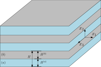
Figure 2. An illustration of an infinite periodic laminate, composed of alternating $a$ and $b$ phases, with initial thicknesses $H^{(a)}$ and $H^{(b)}$, respectively. The electric bias field is along the $x_{2}$ direction.

We assume mechanical traction-free boundary conditions at infinity. Utilizing the jump conditions in the first of (7) and (8), along with the traction-free boundary conditions we have that

$$d_{2}^{\left(b\right)}=d_{2}^{\left(a\right)}=d_{2}, \sigma_{22}^{\left(b\right)}=\sigma_{22}^{\left(a\right)}=0.$$ (44)

From the latter together with the second of Eq. (43) the expressions for the pressure in the phases are

$$p_{0}^{\left(p\right)}=\frac{\mu^{\left(p\right)}}{\lambda^{4}}+\frac{d_{2}^{2}}{\epsilon^{\left(p\right)}}.$$ (45)

Substitution of Eq. (45) into the first of Eq. (43) leads to a relation between the applied Lagrangian electric displacement field $\mathbf{D}=\lambda^{2}\mathbf{d}$ and the resultant stretch ratio, namely

$$\lambda=\left(1+D_{2}^{2}\frac{\breve{\epsilon}}{\bar{\mu}}\right)^{1/6},$$ (46)

where $\breve{\epsilon}=v^{\left(a\right)}/\epsilon^{\left(a\right)}+v^{\left(b\right)}/\epsilon^{\left(b\right)}$ and $\bar{\mu}=\mu^{\left(a\right)}v^{\left(a\right)}+\mu^{\left(b\right)}v^{\left(b\right)}$. The latter appropriately reduces to the corresponding relation for a homogeneous specimen. In terms of the dimensionless quantities $\alpha=\mu^{\left(a\right)}/\mu^{\left(b\right)}$, $\beta=\epsilon^{\left(a\right)}/\epsilon^{\left(b\right)}$, and $\hat{D}=D_{2}/\sqrt{\mu^{\left(b\right)}\epsilon^{\left(b\right)}}$, denoting the shear contrast, permittivity contrast, and normalized Lagrangian electric displacement field, respectively, the stretch ratio is

$$\lambda = \left(1+\hat{D}^{2}\frac{v^{\left(b\right)}+v^{\left(a\right)}\beta^{-1}}{v^{\left(b\right)}+v^{\left(a\right)}\alpha}\right)^{1/6}.$$ (47)

For the above choice of constitutive relation, we also have that Eq. (40) reduces to

$$\mathcal{A}_{11}^{\left(p\right)} = \mathcal{A}_{22}^{\left(p\right)}=\mathcal{A}_{33}^{\left(p\right)}=\frac{1}{\epsilon^{\left(p\right)}},$$ (48)

$$\mathcal{B}_{121}^{\left(p\right)} = \mathcal{B}_{211}^{\left(p\right)}=\mathcal{B}_{323}^{\left(p\right)}=\mathcal{B}_{233}^{\left(p\right)}=\frac{1}{2}\mathcal{B}_{222}^{\left(p\right)}=\frac{1}{\epsilon^{\left(p\right)}}d_{2}^{\left(p\right)},$$ (49)

$$\mathcal{C}_{1111}^{\left(p\right)} = \mathcal{C}_{2121}^{\left(p\right)}=\mathcal{C}_{2323}^{\left(p\right)}=\mathcal{C}_{1313}^{\left(p\right)}=\mathcal{C}_{3333}^{\left(p\right)}=\mu^{\left(p\right)}\lambda^{2},$$ (50)

$$\mathcal{C}_{1212}^{\left(p\right)} = \mathcal{C}_{2222}^{\left(p\right)}=\mathcal{C}_{3232}^{\left(p\right)}=\mu^{\left(p\right)}/\lambda^{4}+\frac{1}{\epsilon^{\left(p\right)}}d_{2}^{\left(p\right)2}.$$ (51)

The response of the laminate to a harmonic excitation superimposed on the aforementioned finite deformation is addressed next. Let $\dot{x}^{\left(p\right)}_{i}$ and $\varphi^{\left(p\right)}$ denote, respectively, the components of the incremental displacement and the incremental electric potential in the phases, such that $\mathrm{\check{\mathbf{e}}}^{\left(p\right)}=-\nabla\varphi^{\left(p\right)}$. The fields sought are to satisfy the incremental equations of motion along with Gauss equation (17) and the incompressibility constraint (18). Following Tiersten (1963), we consider fields that are functions of $x_{2}$ and time alone, independent of $x_{1}$ and $x_{3}$, compatible with the simple-thickness mode (Mindlin, 1955). Consequently, in each phase the governing equations (17) and (18) simplify to

$$\tilde{\mu}^{\left(p\right)}h_{12,2}^{\left(p\right)} =\rho^{\left(p\right)}\dot{x}_{1,tt}^{\left(p\right)},$$ (52a)

$$\left(\tilde{\mu}^{\left(p\right)}-\frac{3}{\epsilon^{\left(p\right)}}d_{2}^{2}+p_{0}^{\left(p\right)}\right)h_{22,2}^{\left(p\right)}-\dot{p}_{0,2}^{\left(p\right)}-2d_{2}\varphi_{,22}^{\left(p\right)} =\rho^{\left(p\right)}\dot{x}_{2,tt}^{\left(p\right)},$$ (52b)

$$\tilde{\mu}^{\left(p\right)}h_{32,2}^{\left(p\right)} =\rho^{\left(p\right)}\dot{x}_{3,tt}^{\left(p\right)},$$ (52c)

and

$$\check{d}_{2,2}^{\left(p\right)} =0,$$ (53a)

$$h_{22}^{\left(p\right)} =0,$$ (53b)

respectively, where $\tilde{\mu}^{\left(p\right)}=\mu^{\left(p\right)}/\lambda^{4}$, $\check{d}_{2}^{\left(p\right)}=-\epsilon^{\left(p\right)}\left(d_{2}\varphi_{,2}^{\left(p\right)}+\frac{2}{\epsilon^{\left(p\right)}}d_{2}h_{22}^{\left(p\right)}\right)$. Substitution of Eq. (53b) into Eq. (53a) reveals that $\varphi_{,22}^{\left(p\right)}=0$, hence the incremental electric potential is linear in $x_{2}$, say $\varphi^{\left(p\right)}=L_{1}^{\left(p\right)}+x_{2}^{\left(p\right)}L_{2}^{\left(p\right)}$, where $L_{1}^{\left(p\right)}$ and $L_{2}^{\left(p\right)}$ are integration constants. More significantly, it implies that the incremental electrical and mechanical fields are not coupled, as Eq. (52b) remains a function of $\mathbf{h}^{\left(p\right)}$ alone, independent of $\varphi^{\left(p\right)}$, together with Eq. (53a) which remains a function of $\varphi^{\left(p\right)}$ alone, independent of $\mathbf{h}^{\left(p\right)}$. Eq. (53b) states that along the thickness the incremental displacement is spatially constant. Together with Eqs. (52a) and (52c) the solution for the incremental problem is

$$\dot{x}^{\left(p\right)}_{1} = \left(U^{\left(p\right)}_{1}\sin k^{\left(p\right)}x_{2}+U^{\left(p\right)}_{2}\cos k^{\left(p\right)}x_{2}\right)e^{-i\omega t},$$

$$\dot{x}^{\left(p\right)}_{2} = U^{\left(p\right)}_{3}e^{-i\omega t},$$ (54)

$$\dot{x}^{\left(p\right)}_{3} = \left(U^{\left(p\right)}_{4}\sin k^{\left(p\right)}x_{2}+U^{\left(p\right)}_{5}\cos k^{\left(p\right)}x_{2}\right)e^{-i\omega t},$$

where $k^{\left(p\right)}=\omega/\bar{c}^{\left(p\right)}$, $\bar{c}^{\left(p\right)}=\tilde{\mu}^{\left(p\right)}/\rho^{\left(p\right)}$, $\omega$ is the angular excitation frequency, and ${U^{\left(p\right)}_{r}}\left(r=1,2,\ldots,5\right)$ are integration constants. Without loss of generality the constants $U^{\left(p\right)}_{3}$ can be set to be zero. The motion described by the solution Eq. (54) corresponds to displacement gradients which retain only shear components. For completeness, the solution for the incremental pressure emerges from Eq. (52b), which reduces to $-\dot{p}_{0,2}^{\left(p\right)}=\rho^{\left(p\right)}\dot{x}_{2,tt}^{\left(p\right)},$ and implies that $\dot{p}_{0}^{\left(p\right)}=P^{\left(p\right)}e^{-i\omega t}$, where $P^{\left(p\right)}$ are integration constants. The incremental state vector of the $n^{th}$ cell takes the form

$$\mathrm{s}_{(n)}^{\left(p\right)}=\left\{\dot{x}^{\left(p\right)}_{n1},\dot{x}^{\left(p\right)}_{n3},\Sigma_{n12}^{\left(p\right)},\Sigma_{n22}^{\left(p\right)},\Sigma_{n32}^{\left(p\right)},\varphi_{n}^{\left(p\right)},\check{d}_{n2}^{\left(p\right)}\right\}{}^{\mathrm{T}}.$$ (55)

The components of transfer matrix $\mathbf{T}_{(n)}^{\left(p\right)}$ relating the top $\mathbf{s}_{t\left(n\right)}^{\left(p\right)}$ and bottom $\mathbf{s}_{b\left(n\right)}^{\left(p\right)}$ state vectors are given in the Appendix. Note that the continuity conditions for $\dot{x}^{\left(p\right)}_{n2}$ is identically satisfied when we set $U^{\left(p\right)}_{3}$ to zero. The corresponding solution of the eigenvalue problem Eq. (34) resulting from the Bloch-Floquet theorem can be expressed in terms of the trigonometric expression

$$k_{B}=\frac{1}{h}\arccos\eta,$$ (56)

where

$$\eta=\frac{1}{2h}\left[\cos k^{\left(b\right)}h^{\left(b\right)}\cos k^{\left(a\right)}h^{\left(a\right)}-\frac{1}{2}\left(k^{\left(b\right)}/k^{\left(a\right)}+k^{\left(a\right)}/k^{\left(b\right)}\right)\sin k^{\left(b\right)}h^{\left(b\right)}\sin k^{\left(a\right)}h^{\left(a\right)}\right],$$ (57)

with $h^{\left(p\right)}=H^{\left(p\right)}/\lambda^{2}$ and $h=h^{\left(a\right)}+h^{\left(b\right)}$. Eq. (56) is an extension of the solution given in Wang et al. (1986) to the class of finitely deformed infinite periodic DE laminates. The dependency on the bias field becomes evident when $\eta$ is rephrased in terms of the electric bias field, the referential geometry and the frequency, namely

$$\eta = \frac{1}{2H}\left(1+D_{2}^{2}\frac{\breve{\epsilon}}{\bar{\mu}}\right)^{1/3}\bigg{[}\cos\frac{\omega\rho^{\left(b\right)}H^{\left(b\right)}}{\mu^{\left(b\right)}\left(1+D_{2}^{2}\frac{\breve{\epsilon}}{\bar{\mu}}\right)^{1/3}}\cos\frac{\omega\rho^{\left(a\right)}H^{\left(a\right)}}{\mu^{\left(a\right)}\left(1+D_{2}^{2}\frac{\breve{\epsilon}}{\bar{\mu}}\right)^{1/3}}$$ (58)

$$-\frac{1}{2}\left(\frac{\alpha\rho^{\left(b\right)}}{\rho^{\left(a\right)}}+\frac{\rho^{\left(a\right)}}{\alpha\rho^{\left(b\right)}}\right)\sin\frac{\omega\rho^{\left(b\right)}H^{\left(b\right)}}{\mu^{\left(b\right)}\left(1+D_{2}^{2}\frac{\breve{\epsilon}}{\bar{\mu}}\right)^{1/3}}\sin\frac{\omega\rho^{\left(a\right)}H^{\left(a\right)}}{\mu^{\left(a\right)}\left(1+D_{2}^{2}\frac{\breve{\epsilon}}{\bar{\mu}}\right)^{1/3}}\bigg{]}.$$

In virtue of the uncoupled nature of the incremental problem, the incremental electric quantities indeed do not appear in Eq. (58). We conclude this section noting that waves of certain frequencies cannot propagate when the pertained solution of $k_{B}$ is complex. These cases will be examined in the following section.

4. Numerical examples

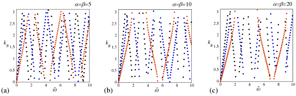
Figure 3. Variations of the Bloch wavenumber $k_{B}$ as functions of the normalized frequency $\hat{\omega}=\omega H/\bar{c}$, for (a) $\alpha=\beta=5$, (b) $\alpha=\beta=10$ and (c) $\alpha=\beta=20$. The red, blue and black curves correspond to $v^{\left(b\right)}=0.2,\ 0.5$ and 0.8, respectively.

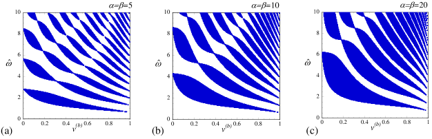
Figure 4. Prohibited frequencies as functions of $v^{\left(b\right)}$ at $\hat{D}=3$, for (a) $\alpha=\beta=5$ and (b) $\alpha=\beta=10$ and (c) $\alpha=\beta=20$.

With the help of a few examples we explore the dispersion relation characterizing the dynamic response of the composite. We examine its dependency on the phases volume fractions and the contrast between the phases shear and dielectric moduli. In particular we are interested in the influence of the electric bias field on the dynamic response of the composite. To this end we make the following choice for the properties of phase $b$

$$\rho^{\left(b\right)}=1000\left[\frac{kg}{m^{3}}\right], \mu^{\left(b\right)}=200\left[KPa\right], \epsilon_{r}^{\left(b\right)}=2,$$ (59)

and determine dispersion diagrams for various choices of phase $a$ properties and volume fractions at different values of the dimensionless bias field $\hat{D}$. In all the forthcoming examples $\rho^{\left(a\right)}=\rho^{\left(b\right)}$ is assumed.

Fig. 3 shows variations of the Bloch wavenumber $k_{B}$ as functions of the normalized frequency $\hat{\omega}=\omega H/\bar{c}$ where $\bar{c}=\sqrt{\bar{\mu}/\bar{\rho}}$, $\bar{\rho}=\rho^{\left(a\right)}v^{\left(a\right)}+\rho^{\left(b\right)}v^{\left(b\right)}$, for a representative value of the bias field $\hat{D}=3$. Figs. 3a, b and c correspond to $\alpha=\beta=5,10$ and 20, respectively. The red, blue and black curves correspond to $v^{\left(b\right)}=0.2,0.5$ and 0.8, respectively. The period of the dispersion curves becomes smaller with an increase of the softer phase volume fraction. An inverse effect is revealed when the contrast is enhanced, that is longer periods for higher values of $\alpha$ and $\beta$.

Fig. 4 displays the regions of prohibited normalized frequencies $\hat{\omega}$ as functions of the matrix volume fraction at a fixed value of the bias field $\hat{D}=3$. Figs. 4a, b and c correspond to $\alpha=\beta=5$, $10$ and $20$, respectively. Herein and henceforth the band-gaps are the blue regions in the plots. We observe how an increase of the softer phase volume fraction results in appearance of additional thinner bands. Conversely, when the contrasts are increased, that is higher values of $\alpha$ and $\beta$, there are fewer thicker bands. The latter is evident in Fig. 5 which displays the prohibited frequencies as functions of $\alpha$ for $v^{\left(b\right)}=0.5$ and $\hat{D}=3$, with different values of $\beta$. Specifically, Fig. 5a corresponds to $\beta=0.1$ and Fig. 5b corresponds to $\beta=10$. Similar trends are observed when the dielectric contrast is investigated. Fig. 6 displays the prohibited frequencies $\hat{\omega}$ as functions of $\beta$ for $v^{\left(b\right)}=0.5$, with different values of $\alpha$. Fig. 6a corresponds to $\alpha=0.1$ and Fig. 6b to $\alpha=10$. Figs. 5 and 6 reveal that whenever the phases have non-monotonous ratios of shear moduli and dielectric contrasts, i.e. $\alpha>1$ and $\beta>1$ or $\alpha<1$ and $\beta>1$, the band gaps become thiner and denser.

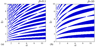
Figure 5. Prohibited frequencies as functions of $\alpha$ at $\hat{D}=3$ and $v^{\left(b\right)}=0.5$, for (a) $\beta=0.1$ and (b) $\beta=10$.

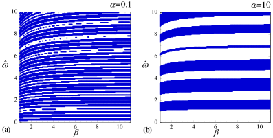
Figure 6. Prohibited frequencies as functions of $\beta$ at $\hat{D}=3$ and $v^{\left(b\right)}=0.5$, for (a) $\alpha=0.1$ and (b) $\alpha=10$.

Fig. 7 illustrates the influence of the bias field by examining the variations of the BGs as functions of the normalized parameter $\hat{D}$. Values of $v^{\left(b\right)}=0.8$ and $\alpha=\beta=5$ were chosen in Fig. 7a, $v^{\left(b\right)}=0.5$ and $\alpha=\beta=10$ in Fig. 7b, and $v^{\left(b\right)}=0.2$ and $\alpha=\beta=20$ in Fig. 7c. The influence of the electric field is evident as the BGs are shifted toward lower frequencies when the field is increased. This phenomena suggests that control of BGs and filtering of desired frequencies are feasible by activating DE laminates with adequate bias electric fields.

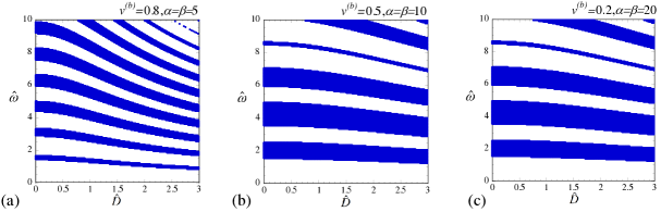
Figure 7. Prohibited frequencies as functions of $\hat{D}$ for (a) $v^{\left(b\right)}=0.8,\alpha=\beta=5$, (b) $v^{\left(b\right)}=0.5,\alpha=\beta=10$ and (c) $v^{\left(b\right)}=0.2,\alpha=\beta=20$.

Finally, we consider realizable laminates made out of commercially available DEs. We examine three materials: VHB-4910 by 3M, ELASTOSIL RT-625 by Wacker, and fluorosilicone 730 by Dow Corning. Approximate physical properties of these elastomers, as reported in the literature (e.g., Kofod and Sommer-Larsen, 2005; Kornbluh and Pelrine, 2008), are summarized in table 1. We investigate different combinations of the two-phase laminate and assume that $v^{\left(b\right)}=v^{\left(a\right)}$.

Table 1. Physical properties of commercially available DEs.

Material	density $\left[\rm{kg}/{m^{3}}\right]$	shear modulus $\left[\rm kPa\right]$	relative dielectric
			constant
VHB-4910	960	406	4.7
ELASTOSIL RT-625	1020	342	2.7
Fluorosilicone 730	1400	167	6.9

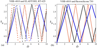
Figure 8. Variations of the Bloch wavenumber $k_{B}$ as functions of the normalized frequency $\hat{\omega}=\omega H/\bar{c}$ for combinations of VHB-4910 with (a) ELASTOSIL RT-625, and with (b) fluorosilicone 730.

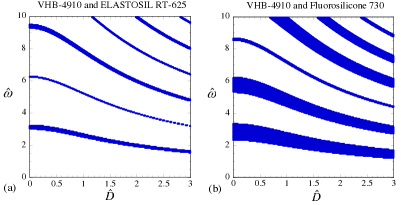
Figure 9. Prohibited frequencies as functions of $\hat{D}$ for combinations of VHB-4910 with (a) ELASTOSIL RT-625, and (b) fluorosilicone 730.

Fig. 8 displays the dispersion relation in terms of Bloch wavenumber $k_{B}$ as a function of the normalized frequency $\hat{\omega}$. Fig. 8a corresponds to a combination of VHB-4910 and ELASTOSIL RT-625, while Fig. 8b to VHB-4910 and fluorosilicone 730. In terms of the dimensionless parameters in Fig. 8a $\alpha=1.19$ and $\beta=1.74$, and in Fig. 8b $\alpha=2.44$ and $\beta=0.68$. The blue, black and red curves correspond to $\hat{D}=0.5,1$ and 1.5, respectively.

Fig. 9 shows the prohibited frequencies as functions of the bias field in terms of the dimensionless bias field $\hat{D}$. Again, Fig. 9a corresponds to the combination of VHB-4910 and ELASTOSIL RT-625, and Fig.9b c to VHB-4910 and fluorosilicone 730. Wider bands are depicted in Fig. 9b in comparison with Fig. 9a, since the latter corresponds to a laminate with higher shear contrast between the phases.

5. Concluding remarks

Motivated by the ability of DEs to undergo large deformations and change their mechanical and electrical properties when electrostatically excited, the feasibility of inducing and controlling BGs by the electrical bias field is explored. To this end we first considered the static response of an infinite periodic laminate to a bias electric displacement field. Subsequently, the propagation of small waves superposed on the pre-strained composite is addressed. Applications of the transfer matrix method along with the Bloch-Floquet theorem resulted in a dispersion relation between the waves frequencies, the phase velocities, and the Bloch-parameter. Numerical analysis of these relations was conducted for specific two-phase laminates in order to examine how the stop-bands, associated with complex Bloch-parameter, vary as functions of the geometrical, mechanical and electric properties of the laminate. Most importantly, this analysis reveals the influence of the electrostatic bias fields on the BGs. Our findings demonstrate how when the concentration of the softer phase in increased, the bands become thinner and additional band gaps the appear. An inverse effect is observed when the contrast between the phases properties is increased (larger values of $\alpha$ and $\beta$). The primary conclusion of our analysis is depicted in Fig. 7, demonstrating how variations in the bias electric displacement field lead to modifications in the width and shifts in the range of the prohibited frequencies. We note that for lower values of $\alpha$ and $\beta$ the effect of the bias electric field becomes more evident in the sense that the shift in the BGs range is larger. From practical viewpoint point, while stopping larger bands of frequencies is feasible by choosing a higher contrast, lower contrasts will allow to actively adjust the desired band at a higher precision. The analysis was concluded with two examples in which we chose phases properties to be identical to those of commercially available DEs. The results show how tunable stop-bands are achievable by properly adjusting the electrostatic bias field.

Appendix A The transfer matrix

The components of the transfer matrices $\mathrm{T}^{\left(p\right)}_{(n)}$ appearing in section 3:

$$T_{11}^{\left(p\right)}=T_{22}^{\left(p\right)}=T_{33}^{\left(p\right)}=T_{55}^{\left(p\right)}=\cos k^{\left(p\right)}h^{\left(p\right)},$$ (60)

$$T_{13}^{\left(p\right)}=T_{52}^{\left(p\right)}=\sin k^{\left(p\right)}h^{\left(p\right)}/\bar{\mu}k^{\left(p\right)},$$ (61)

$$T_{31}^{\left(p\right)}=T_{13}^{\left(p\right)}=T_{52}^{\left(p\right)}=-\bar{\mu}k^{\left(p\right)}\sin k^{\left(p\right)}h^{\left(p\right)},$$ (62)

$$T_{66}^{\left(p\right)}=-h^{\left(p\right)}/d\epsilon^{\left(p\right)},$$ (63)

$$T_{44}^{\left(p\right)}=T_{66}^{\left(p\right)}=1,$$ (64)

with all the remaining components being zero.

References

• (1)
• Adler (1990) Adler, E. L. (1990). Matrix methods applied to acoustic waves in multilayers, Ultrasonics, Ferroelectrics and Frequency Control, IEEE Transactions on 37: 485–490.
• Bertoldi and Gei (2011) Bertoldi, K. and Gei, M. (2011). Instabilities in multilayered soft dielectrics, J. Mech. Phys. Solids 59: 18–42.
• deBotton et al. (2007) deBotton, G., Tevet-Deree, L. and Socolsky, E. A. (2007). Electroactive heterogeneous polymers: analysis and applications to laminated composites, Mechanics of Advanced Materials and Structures 14: 13–22.
• Dorfmann and Ogden (2005) Dorfmann, A. and Ogden, R. W. (2005). Nonlinear electroelasticity, Acta. Mech. 174: 167–183.
• Dorfmann and Ogden (2010) Dorfmann, A. and Ogden, R. W. (2010). Electroelastic waves in a finitely deformed electroactive material, IMA J Appl Math 75: 603–636.
• Gei et al. (2004) Gei, M., Bigoni, D. and Franceschini, G. (2004). Thermoelastic small-amplitude wave propagation in nonlinear elastic multilayers, Mathematics and Mechanics of Solids 9: 555–568.
• Gei et al. (2009) Gei, M., Movchan, A. B. and Bigoni, D. (2009). Band-gap shift and defect-induced annihilation in prestressed elastic structures, Journal of Applied Physics 105: 063507.
• Gei et al. (2011) Gei, M., Roccabianca, S. and Bacca, M. (2011). Controlling band gap in electroactive polymer-based structures, IEEE-ASME Transactions on Mechatronics 16: 102–107.
• Kittel (2005) Kittel, C. (2005). Introduction to Solid State Physics, John Wiley & Sons, Inc., Hoboken, NJ.
• Kofod (2008) Kofod, G. (2008). The static actuation of dielectric elastomer actuators: how does pre-stretch improve actuation?, J. Phys. D-Appl. Phys. 41: 215405.
• Kofod and Sommer-Larsen (2005) Kofod, G. and Sommer-Larsen, P. (2005). Silicone dielectric elastomer actuators: Finite-elasticity model of actuation, Sensors and Actuators A: Physical 122: 273–283.
• Kohn et al. (1972) Kohn, W., Krumhansl, J. A. and Lee, E. H. (1972). Variational methods for dispersion relations and elastic properties of composite materials, J. Appl. Mech., Trans. ASME 39(2): 327–336.
• Kornbluh and Pelrine (2008) Kornbluh, R. and Pelrine, R. (2008). High-performance acrylic and silicone elastomers, in F. Carpi, D. De Rossi, R. Kornbluh, R. Pelrine and P. Sommer-Larsen (eds), Dielectric Elastomers as Electromechanical Transducers, Elsevier, Oxford, UK, chapter 4, pp. 33–42.
• Kushwaha et al. (1993) Kushwaha, M. S., Halevi, P., Dobrzynski, L. and Djafari-Rouhani, B. (1993). Acoustic band structure of periodic elastic composites, Phys. Rev. Lett. 71: 2022–2025.
• Kushwaha et al. (1994) Kushwaha, M. S., Halevi, P., Martínez, G., Dobrzynski, L. and Djafari-Rouhani, B. (1994). Theory of acoustic band structure of periodic elastic composites, Phys. Rev. B 49(4): 2313–2322.
• Mindlin (1955) Mindlin, R. D. (1955). An Introduction to the Mathematical Theory of Vibrations of Elastic Plates, U.S. Army Signal Corps Engineering Laboratories, Fort Monmouth, NJ.
• Pelrine et al. (2000) Pelrine, R., Kornbluh, R., Pei, Q.-B. and Joseph, J. (2000). High-speed electrically actuated elastomers with strain greater than 100%, Science 287: 836–839.
• Ponte Castañeda and Siboni (2011) Ponte Castañeda, P. and Siboni, M. H. (2011). A finite-strain constitutive theory for electro-active polymer composites via homogenization, Int. J. Nonlinear Mech. p. (10.1016/j.ijnonlinmec.2011.06.012).
• Rudykh and deBotton (2011) Rudykh, S. and deBotton, G. (2011). Stability of anisotropic electroactive polymers with application to layered media, Z. angew. Math. Phys. (ZAMP) pp. (10.1007/s00033–011–0136–1).
• Sabina and Willis (1988) Sabina, F. J. and Willis, J. R. (1988). A simple self-consistent analysis of wave propagation in particulate composites, Wave Motion 10: 127–142.
• Shmuel et al. (2011) Shmuel, G., Gei, M. and deBotton, G. (2011). The rayleigh-lamb wave propagation in dielectric elastomer layers subjected to large deformations, Int. J. Nonlinear Mech. p. (doi:10.1016/j.ijnonlinmec.2011.06.013).
• Sigalas and Economou (1996) Sigalas, M. M. and Economou, E. N. (1996). Attenuation of multiple scattered sound, Europhysics Letters 36: 241–246.
• Tanaka and Tamura (1998) Tanaka, Y. and Tamura, S. (1998). Surface acoustic waves in two-dimensional periodic elastic structures, Phys. Rev. B 58: 7958–7965.
• Tian et al. (2012) Tian, L., Tevet-Deree, L., deBotton, G. and Bhattacharya, K. (2012). Dielectric elastomer composites, J. Mech. Phys. Solids 60: 181–198.
• Tiersten (1963) Tiersten, H. F. (1963). Thickness vibrations of piezoelectric plates, J. Acoust. Soc. Am. 35: 53–58.
• Wang and Auld (1985) Wang, Y. and Auld, B. A. (1985). Acoustic wave propagation in one-dimensional periodic composites, in B. R. McAvoy (ed.), IEEE 1985 Ultrasonics Symposium, pp. 637–641.
• Wang and Auld (1986) Wang, Y. and Auld, B. A. (1986). Numerical analysis of bloch theory for acoustic wave propagation in one-dimensional periodic composites, Applications of Ferroelectrics. 1986 Sixth IEEE International Symposium on, pp. 261–264.
• Wang et al. (1986) Wang, Y., Schmidt, E. and Auld, B. A. (1986). Acoustic wave transmission through one-dimensional PZT-epoxy composites, in B. R. McAvoy (ed.), IEEE 1986 Ultrasonics Symposium, pp. 685–690.
• Ziegler (1977) Ziegler, F. (1977). Wave propagation in periodic and disordered layered composite elastic materials, Int. J. Solids Struct. 13: 293–305.