Newton trees for ideals in two variables and applications

Abstract.

We introduce an efficient way, called Newton algorithm, to study arbitrary ideals in ${\mathbb{C}}[[x,y]]$, using a finite succession of Newton polygons. We codify most of the data of the algorithm in a useful combinatorial object, the Newton tree. For instance when the ideal is of finite codimension, invariants like integral closure and Hilbert-Samuel multiplicity were already combinatorially determined in the very special cases of monomial or non degenerate ideals, using the Newton polygon of the ideal. With our approach, we can generalize these results to arbitrary ideals. In particular the Rees valuations of the ideal will correspond to the so-called dicritical vertices of the tree, and its Hilbert-Samuel multiplicity has a nice and easily computable description in terms of the tree.

1. Introduction

Let ${\mathcal{I}}$ be an ideal in ${\mathbb{C}}[[x,y]]$, given by a system of generators ${\mathcal{I}}=(f_{1},\cdots,f_{r})$. How to compute its integral closure $\overline{{\mathcal{I}}}$, its Hilbert-Samuel multiplicity $e({\mathcal{I}})$ (when $I$ is of finite codimension) and so on?

The simplest case already studied is the case of monomial ideals, which means ideals generated by monomials. In this case, the results are expressed in terms of the Newton polygon of the ideal. If $f=\sum c_{{\alpha},{\beta}}x^{{\alpha}}y^{{\beta}}\in{\mathbb{C}}[[x,y]]$, denote ${\operatorname{Supp}}f=\{({\alpha},{\beta})\in{\mathbb{N}}\times{\mathbb{N}}\mid c_{{\alpha},{\beta}}\neq 0\}.$ The Newton polygon $\mathcal{N}({\mathcal{I}})$ is the union of the $1$-dimensional compact faces of the convex hull $\Delta({\mathcal{I}})$ of $\cup_{i}{\operatorname{Supp}}f_{i}$. In particular the Zariski decomposition of $\overline{{\mathcal{I}}}$ takes the easy form

(1.1) $$\overline{{\mathcal{I}}}=x^{k}y^{l}\prod_{S\in\mathcal{N}({\mathcal{I}})}{\mathcal{I}}_{(p_{S},q_{S})}^{\delta_{S}},$$

where $S$ is a face of $\mathcal{N}({\mathcal{I}})$ with equation $p_{S}{\alpha}+q_{S}{\beta}=N_{S}$, with $(p_{S},q_{S})=1$ and $\delta_{S}=N_{S}/(p_{S}q_{S})$, and ${\mathcal{I}}_{(p_{S},q_{S})}$ is the integrally closed simple ideal such that its Newton polygon has a unique face with equation $p_{S}{\alpha}+q_{S}{\beta}=N_{S}/\delta_{S}$. Moreover, if ${\mathcal{I}}$ has finite codimension, we have

$$e({\mathcal{I}})=\sum_{S\in\mathcal{N}({\mathcal{I}})}N_{S}\delta_{S},$$

which is twice the area of the region ${\mathbb{R}}^{2}_{+}\setminus\Delta({\mathcal{I}})$ delimited by the coordinate axes and the Newton polygon. Such results have been generalized in the case of non degenerate ideals of finite codimension.

In this article we prove for instance that such results can be generalized to any ideal, if we use a finite number of Newton polygons instead of one. The method we use is inspired by Newton’s method to find roots of $f\in{\mathbb{C}}[[x,y]]$. We call it Newton algorithm. We codify the algorithm in two ways: the Newton tree which keeps the information of the successive Newton polygons we encounter in the algorithm, and the Newton process which keeps the information of all the Newton maps we use in the algorithm. From the Newton process, we can recover the Newton tree but not the other way around. We prove that the Newton process characterizes the integral closure of the ideal and allows to give its Zariski decomposition, whereas the Newton tree suffices to compute the Hilbert-Samuel multiplicity.

It should be noted that the Newton algorithm has been very efficient in the proof of the monodromy conjecture for quasiordinary power series, see [1][2].

The paper is organized as follows. In the next section we introduce the Newton algorithm, as a composition of Newton maps, that transforms an arbitrary ideal ${\mathcal{I}}$ of ${\mathbb{C}}[[x,y]]$ into a principal ‘monomial-like’ ideal. We associate a notion of depth to ${\mathcal{I}}$, being roughly the length of this algorithm, and we say that ${\mathcal{I}}$ is non degenerate if the depth of ${\mathcal{I}}$ is at most one. In the cases where ${\mathcal{I}}$ is principal or of finite codimension, this is consistent with usual notions of non degeneracy. In section 3 we describe the Newton tree and its combinatorial properties. In particular we compare the Newton tree of a non-principal ideal with the Newton tree of a generic curve of that ideal. The Newton process is treated in section 4, where we show that an ideal has the same Newton process as its integral closure. In section 5 we then study several invariants of an ideal ${\mathcal{I}}$ of ${\mathbb{C}}[[x,y]]$ in terms of its Newton tree or process. First we identify the Rees valuations of ${\mathcal{I}}$ with certain elements in the Newton tree/process. This leads to the proof of the fact that two ideals have the same Newton process if and only if they have the same integral closure, using a result of Rees and Sharp. Further we interpret Zariski’s decomposition of ${\mathcal{I}}$, as a product of principal and simple integrally closed ideals of finite codimension, in terms of the Newton process, generalizing (1.1). Finally we compute, when ${\mathcal{I}}$ has finite codimension, its multiplicity, its Łojasiewicz exponent and its Hilbert-Samuel multiplicity $e({\mathcal{I}})$ from the Newton tree, and we show an alternative formula for $e({\mathcal{I}})$ in terms of the area defined by the successive Newton polygons encountered in the Newton algorithm.

2. Newton Algorithm for an ideal

2.1. Newton polygon

For any set $E\subset{\mathbb{N}}\times{\mathbb{N}}$, denote by $\Delta(E)$ the smallest convex set containing $E+{\mathbb{R}}_{+}^{2}=\{a+b\mid a\in E,b\in{\mathbb{R}}_{+}^{2}\}$. A set $\Delta\subset{\mathbb{R}}^{2}$ is a Newton diagram if there exists a set $E\subset{\mathbb{N}}\times{\mathbb{N}}$ such that $\Delta=\Delta(E)$. The smallest set $E_{0}\subset{\mathbb{N}}\times{\mathbb{N}}$ such that $\Delta=\Delta(E_{0})$ is called the set of vertices of a Newton diagram $\Delta$; it is a finite set. Let $E_{0}=\{v_{0},\cdots,v_{m}\}$, with $v_{i}=({\alpha}_{i},{\beta}_{i})\in{\mathbb{N}}\times{\mathbb{N}}$ for $i=0,\cdots,m$, and ${\alpha}_{i-1}<{\alpha}_{i}$, ${\beta}_{i-1}>{\beta}_{i}$ for $i=1,\cdots,m$. For $i\in\{1,\cdots,m\}$, denote $S_{i}=[v_{i-1},v_{i}]$ and by $l_{S_{i}}$ the line supporting the segment $S_{i}$. We call ${\mathcal{N}}({\Delta})=\cup_{1\leq i\leq m}S_{i}$ the Newton polygon of ${\Delta}$ and the $S_{i}$ its faces. The Newton polygon ${\mathcal{N}}({\Delta})$ is empty if and only if $E_{0}=\{v_{0}=({\alpha}_{0},{\beta}_{0})\}$. The integer $h({\Delta})={\beta}_{0}-{\beta}_{m}$ is called the height of ${\Delta}$. Let

$$f(x,y)=\sum_{({\alpha},{\beta})\in{\mathbb{N}}\times{\mathbb{N}}}c_{{\alpha},{\beta}}x^{{\alpha}}y^{{\beta}}\in{\mathbb{C}}[[x,y]].$$

We define the support of $f$ as

$${\operatorname{Supp}}f=\{({\alpha},{\beta})\in{\mathbb{N}}\times{\mathbb{N}}\mid c_{{\alpha},{\beta}}\neq 0\}.$$

We denote $\Delta(f)=\Delta({\operatorname{Supp}}f)$ and ${\mathcal{N}}(f)={\mathcal{N}}({\Delta}(f))$. Let $l$ be a line in ${\mathbb{R}}^{2}$. We define the initial part of $f$ with respect to $l$ as

$${\operatorname{in}}(f,l)=\sum_{({\alpha},{\beta})\in l}c_{{\alpha},{\beta}}x^{{\alpha}}y^{{\beta}}.$$

If the line $l$ has equation $p{\alpha}+q{\beta}=N$, with $(p,q)\in({\mathbb{N}}^{*})^{2}$ and $\gcd(p,q)=1$, then ${\operatorname{in}}(f,l)$ is zero or a monomial or, if $l=l_{S}$ for some segment $S$ of ${\mathcal{N}}({\Delta})$, of the form

$${\operatorname{in}}(f,l)=x^{a_{l}}y^{b_{l}}F_{S}(x^{q},y^{p}),$$

where $(a_{l},b_{l})\in{\mathbb{N}}^{2}$ and

$$F_{S}(x,y)=c\prod_{1\leq i\leq n}(y-{\mu}_{i}x)^{\nu_{i}},$$

with $c\in{\mathbb{C}}^{*}$, $n\in{\mathbb{N}}^{*}$, ${\mu}_{i}\in{\mathbb{C}}^{*}$ (all different) and $\nu_{i}\in{\mathbb{N}}^{*}$.

For example if $f(x,y)=(x^{2}+y^{3})^{2}+\sum_{i\geq 1}x^{i}y^{5i}$, then ${\mathcal{N}}(f)=\{S\}$, where $l_{S}$ has equation $3\alpha+2\beta=12$ and ${\operatorname{in}}(f,l_{S})=(x^{2}+y^{3})^{2}$.

Now let ${\mathcal{I}}=(f_{1},\cdots,f_{r})$ be a non-trivial ideal in ${\mathbb{C}}[[x,y]]$. We define

$${\Delta}({\mathcal{I}})={\Delta}(\cup_{1\leq i\leq r}{\operatorname{Supp}}f_{i})\quad\text{and}\quad{\mathcal{N}}({\mathcal{I}})={\mathcal{N}}({\Delta}({\mathcal{I}})).$$

When ${\mathcal{I}}=(f)$ we simply write ${\Delta}(f)$ and ${\mathcal{N}}(f)$. For a segment $S$ of ${\mathcal{N}}({\mathcal{I}})$ we denote by ${\operatorname{in}}({\mathcal{I}},S)$ the ideal generated by the ${\operatorname{in}}(f_{i},l_{S}),1\leq i\leq r$, and call it the initial ideal of ${\mathcal{I}}$ with respect to $S$.

Lemma 2.1.

The sets ${\Delta}({\mathcal{I}})$ and ${\mathcal{N}}({\mathcal{I}})$ and the ideals ${\operatorname{in}}({\mathcal{I}},S)$ depend only on ${\mathcal{I}}$, not on a system of generators of ${\mathcal{I}}$.

Proof.

If ${\mathcal{I}}=(f_{1},\cdots,f_{m})=(g_{1},\cdots,g_{s})$, then we have for $j=1,\cdots,s$ that

$$g_{j}(x,y)=\sum_{i}h_{ij}(x,y)f_{i}(x,y),$$

where the $h_{ij}\in{\mathbb{C}}[[x,y]]$. Then

$${\operatorname{Supp}}\,g_{j}\subset\cup_{i}{\operatorname{Supp}}f_{i}+{\mathbb{R}}_{+}^{2}$$

for all $j$, and hence

$$\cup_{j}{\operatorname{Supp}}\,g_{j}+{\mathbb{R}}_{+}^{2}\subset\cup_{i}{\operatorname{Supp}}f_{i}+{\mathbb{R}}_{+}^{2}.$$

By symmetry we can conclude that indeed

$$\cup_{j}{\operatorname{Supp}}\,g_{j}+{\mathbb{R}}_{+}^{2}=\cup_{i}{\operatorname{Supp}}f_{i}+{\mathbb{R}}_{+}^{2}.$$

Moreover, since any such segment $S$ is a face of ${\mathcal{N}}({\mathcal{I}})$, we have for $j=1,\cdots,s$ that

$${\operatorname{in}}(g_{j},l_{S})=\sum_{i}h_{ij}(0,0)\,{\operatorname{in}}(f_{i},l_{S}),$$

and we can conclude analogously. ∎

Remark 2.2.

The proof of the lemma shows that ${\Delta}({\mathcal{I}})={\Delta}(\cup_{f\in{\mathcal{I}}}{\operatorname{Supp}}f)$.

Remark 2.3.

The Newton polygon of an ideal is empty if and only if the ideal is principal, generated by a monomial.

Let $S$ be a face of ${\mathcal{N}}({\mathcal{I}})$ and $p_{S}{\alpha}+q_{S}{\beta}=N_{S}$ be the equation of $l_{S}$, with $\gcd(p_{S},q_{S})=1$ as before. Then ${\operatorname{in}}({\mathcal{I}},S)$ is of the form

(2.1) $${\operatorname{in}}({\mathcal{I}},S)=\left(x^{a_{S}}y^{b_{S}}F_{{\mathcal{I}},S}(x^{q_{S}},y^{p_{S}})\right)$$

or

(2.2) $${\operatorname{in}}({\mathcal{I}},S)=x^{a_{S}}y^{b_{S}}F_{{\mathcal{I}},S}(x^{q_{S}},y^{p_{S}})\big{(}k_{1}(x^{q_{S}},y^{p_{S}}),\cdots,k_{s}(x^{q_{S}},y^{p_{S}})\big{)}$$

with $s\geq 2$, where $F_{{\mathcal{I}},S},k_{1},\cdots,k_{s}$ are homogeneous polynomials, $F_{{\mathcal{I}},S}$ is not divisible by $x$ or $y$ and $k_{1},\cdots,k_{s}$ are coprime and of the same degree $d_{S}$. In the first case we put $d_{S}=0$. The polynomial $F_{{\mathcal{I}},S}$, monic in $y$, is called the face polynomial (it can be identically one). A face $S$ is called a dicritical face if ${\operatorname{in}}({\mathcal{I}},S)$ is not a principal ideal. Thus it is dicritical if and only if $d_{S}\geq 1$.

The following equality is an immediate consequence of the definitions.

Lemma 2.4.

Let ${\mathcal{I}}$ be a non-trivial ideal in ${\mathbb{C}}[[x,y]]$. Write the face polynomial of each face $S$ of its Newton polygon ${\mathcal{N}}({\mathcal{I}})$ in the form

$$F_{{\mathcal{I}},S}(x,y)=\prod_{1\leq i\leq n_{S}}(y-{\mu}_{S,i}x)^{\nu_{S,i}},$$

where $n_{S}\in{\mathbb{N}}$, ${\mu}_{S,i}\in{\mathbb{C}}^{*}$ (all different) and $\nu_{S,i}\in{\mathbb{N}}^{*}$. Then the height $h$ of ${\Delta}({\mathcal{I}})$ satisfies

(2.3) $$h=\sum_{S}p_{S}\left(d_{S}+\sum_{1\leq i\leq n_{S}}\nu_{S,i}\right).$$

2.2. Newton maps

Definition 2.5.

Let $(p,q)\in({\mathbb{N}}^{*})^{2}$ with $\gcd(p,q)=1$. Take $(p^{\prime},q^{\prime})\in{\mathbb{N}}^{2}$ such that $pp^{\prime}-qq^{\prime}=1$. Let $\mu\in{\mathbb{C}}^{*}$. Define

$$\begin{matrix}&{\sigma}_{(p,q,\mu)}&:&{\mathbb{C}}[[x,y]]&\longrightarrow&{\mathbb{C}}[[x_{1},y_{1}]]\\ &&&f(x,y)&\mapsto&f(\mu^{q^{\prime}}x_{1}^{p},x_{1}^{q}(y_{1}+\mu^{p^{\prime}})).\end{matrix}$$

We say that the map ${\sigma}_{(p,q,\mu)}$ is a Newton map.

Remark 2.6.

(1) The numbers $(p^{\prime},q^{\prime})$ are introduced only to avoid taking roots of complex numbers.

(2) Let $(p^{\prime},q^{\prime})$ be such that $pp^{\prime}-qq^{\prime}=1$. For $i\in{\mathbb{N}}$, we have

$$f\left(\mu^{q^{\prime}+ip}x_{1}^{p},x_{1}^{q}(y_{1}+\mu^{p^{\prime}+iq})\right)=f\left(\mu^{q^{\prime}}(\mu^{i}x_{1})^{p},(\mu^{i}x_{1})^{q}((\mu^{-iq}y_{1})+\mu^{p^{\prime}})\right),$$

which shows that the change of $(p^{\prime},q^{\prime})$ into $(p^{\prime}+iq,q^{\prime}+ip)$ corresponds to the change of coordinates $(x_{1},y_{1})\mapsto(\mu^{i}x_{1},\mu^{-iq}y_{1})$.

In the sequel we will always assume that $p^{\prime}\leq q$ and $q^{\prime}<p$. This will make procedures canonical.

Lemma 2.7.

Let $f(x,y)\in{\mathbb{C}}[[x,y]]$, $f\neq 0$ and ${\sigma}_{(p,q,\mu)}(f)(x_{1},y_{1})=f_{1}(x_{1},y_{1})\in{\mathbb{C}}[[x_{1},y_{1}]]$.

1. If there does not exist a face $S$ of ${\mathcal{N}}(f)$ whose supporting line has equation $p{\alpha}+q{\beta}=k$ with $k\in{\mathbb{N}}$, then

   $$f_{1}(x_{1},y_{1})=x_{1}^{m}u(x_{1},y_{1})$$

   with $m\in{\mathbb{N}}$, $u(x_{1},y_{1})\in{\mathbb{C}}[[x_{1},y_{1}]]$ and $u(0,0)\neq 0$.

2. If there exists a face $S$ of ${\mathcal{N}}(f)$ whose supporting line has equation $p{\alpha}+q{\beta}=k_{0}$ for some $k_{0}\in{\mathbb{N}}$, and if $F_{S}(1,\mu)\neq 0$, then

   $$f_{1}(x_{1},y_{1})=x_{1}^{k_{0}}u(x_{1},y_{1})$$

   with $u(x_{1},y_{1})\in{\mathbb{C}}[[x_{1},y_{1}]]$ and $u(0,0)\neq 0$.

3. If there exists a face $S$ of ${\mathcal{N}}(f)$ whose supporting line has equation $p{\alpha}+q{\beta}=k_{0}$ for some $k_{0}\in{\mathbb{N}}$, and if $F_{S}(1,\mu)=0$, then

   $$f_{1}(x_{1},y_{1})=x_{1}^{k_{0}}g_{1}(x_{1},y_{1})$$

   with $g_{1}(x_{1},y_{1})\in{\mathbb{C}}[[x_{1},y_{1}]]$ and $g_{1}(0,0)=0,g_{1}(0,y_{1})\neq 0$.

Proof.

Let

$$f(x,y)=\sum_{({\alpha},{\beta})\in{\mathbb{N}}^{2}}c_{{\alpha},{\beta}}x^{{\alpha}}y^{{\beta}}\in{\mathbb{C}}[[x,y]];$$

we write

$$f(x,y)=\sum_{k\in{\mathbb{N}}}\sum_{p{\alpha}+q{\beta}=k}c_{{\alpha},{\beta}}x^{{\alpha}}y^{{\beta}}.$$

We have for all $k\in{\mathbb{N}}$ that

$$\sum_{p{\alpha}+q{\beta}=k}c_{{\alpha},{\beta}}(\mu^{q^{\prime}}x_{1}^{p})^{{\alpha}}(x_{1}^{q}(y_{1}+\mu^{p^{\prime}}))^{{\beta}}=x_{1}^{k}\sum_{p{\alpha}+q{\beta}=k}c_{{\alpha},{\beta}}\mu^{q^{\prime}{\alpha}}(y_{1}+\mu^{p^{\prime}})^{{\beta}}.$$

If $k_{0}$ is the smallest $k$ such that $\sum_{p{\alpha}+q{\beta}=k}c_{{\alpha},{\beta}}x^{{\alpha}}y^{{\beta}}\neq 0$ (that is, such that at least one $c_{{\alpha},{\beta}}$ is nonzero), then

$$f_{1}(x_{1},y_{1})=x_{1}^{k_{0}}\left(\sum_{k\geq k_{0}}x_{1}^{k-k_{0}}\sum_{p{\alpha}+q{\beta}=k}c_{{\alpha},{\beta}}\mu^{q^{\prime}{\alpha}}(y_{1}+\mu^{p^{\prime}})^{{\beta}}\right).$$

If there does not exist a face of ${\mathcal{N}}(f)$ whose supporting line has equation $p{\alpha}+q{\beta}=k_{0}$, then for $k=k_{0}$ there is only one nonzero $c_{{\alpha},{\beta}}$ in the sum above, hence

$$f_{1}(x_{1},y_{1})=c_{{\alpha},{\beta}}x_{1}^{k_{0}}\mu^{q^{\prime}{\alpha}}(y_{1}+\mu^{p^{\prime}})^{{\beta}}+x_{1}^{k_{0}+1}(\cdots)$$

and, since $\mu\neq 0$, we see that $f_{1}(x_{1},y_{1})=x_{1}^{k_{0}}u(x_{1},y_{1})$ with $u(0,0)\neq 0$.

If there exists a face $S$ of ${\mathcal{N}}(f)$ whose supporting line has equation $p{\alpha}+q{\beta}=k_{0}$, we write ${\operatorname{in}}(f,l_{S})=x^{a}y^{b}F_{S}(x^{q},y^{p})$ as above and $F_{S}(x,y)=c\prod_{i}(y-\mu_{i}x)^{\nu_{i}}$. Then $f_{1}(x_{1},y_{1})$ is of the form

$$f_{1}(x_{1},y_{1})=x_{1}^{k_{0}}\left(c\mu^{q^{\prime}a}(y_{1}+\mu^{p^{\prime}})^{b}F_{S}(\mu^{qq^{\prime}},(y_{1}+\mu^{p^{\prime}})^{p})+\sum_{k>k_{0}}x_{1}^{k-k_{0}}\sum_{p{\alpha}+q{\beta}=k}c_{{\alpha},{\beta}}\mu^{q^{\prime}{\alpha}}(y_{1}+\mu^{p^{\prime}})^{{\beta}})\right),$$

where

$$F_{S}(\mu^{qq^{\prime}},(y_{1}+\mu^{p^{\prime}})^{p})=\prod_{i}((y_{1}+\mu^{p^{\prime}})^{p}-\mu_{i}\mu^{qq^{\prime}})^{\nu_{i}}=F_{S}(1,\mu)\mu^{qq^{\prime}\sum_{i}\nu_{i}}+y_{1}G_{S}(y_{1})$$

with $G_{S}(y_{1})\in{\mathbb{C}}[y_{1}]$ and $G_{S}(y_{1})\neq 0$. So, if $F_{S}(1,\mu)\neq 0$, then $f_{1}(x_{1},y_{1})=x_{1}^{k_{0}}u(x_{1},y_{1})$ with $u(0,0)\neq 0$, and if $F_{S}(1,\mu)=0$, then $f_{1}(x_{1},y_{1})=x_{1}^{k_{0}}g_{1}(x_{1},y_{1})$ with $g_{1}(0,0)=0$.

Note that $F_{S}(1,\mu)=0$ if and only if $\mu=\mu_{i}$ for some $i$ and $g_{1}(0,y_{1})=y_{1}^{\nu_{i}}+\cdots$, where $\cdots$ means higher degree terms in $y_{1}$. ∎

Remark 2.8.

In the first and second case of Lemma 2.7, the Newton polygon of $f_{1}$ is empty. In the third case, the height of the Newton diagram of $f_{1}$ is less than or equal to the multiplicity of $\mu$ as root of $F_{S}(1,X)$.

Let ${\mathcal{I}}=(f_{1},\cdots,f_{r})$ be a non-trivial ideal in ${\mathbb{C}}[[x,y]]$. Let ${\sigma}_{(p,q,\mu)}$ be a Newton map. We denote by ${\sigma}_{(p,q,\mu)}({\mathcal{I}})$ the ideal in ${\mathbb{C}}[[x_{1},y_{1}]]$ generated by the ${\sigma}_{(p,q,\mu)}(f_{i})$ for $i=1,\cdots,r$. Since a Newton map is a ring homomorphism, this ideal does not depend on the choice of the generators of ${\mathcal{I}}$.

Lemma 2.9.

Let ${\mathcal{I}}$ be a non-trivial ideal in ${\mathbb{C}}[[x,y]]$ and ${\sigma}_{(p,q,\mu)}({\mathcal{I}})={\mathcal{I}}_{1}$.

1. If there does not exist a face $S$ of ${\mathcal{N}}({\mathcal{I}})$ whose supporting line has equation $p{\alpha}+q{\beta}=N$ with $N\in{\mathbb{N}}$, then the ideal ${\mathcal{I}}_{1}$ is principal, generated by a power of $x_{1}$.

2. If there exists a face $S$ of ${\mathcal{N}}({\mathcal{I}})$ whose supporting line has equation $p{\alpha}+q{\beta}=N_{0}$ for some $N_{0}\in{\mathbb{N}}$, and if $F_{{\mathcal{I}},S}(1,\mu)\neq 0$, then ${\mathcal{I}}_{1}=(x_{1}^{N_{0}})$.

3. If there exists a face $S$ of ${\mathcal{N}}({\mathcal{I}})$ whose supporting line has equation $p{\alpha}+q{\beta}=N_{0}$ for some $N_{0}\in{\mathbb{N}}$, and if $F_{{\mathcal{I}},S}(1,\mu)=0$, then ${\mathcal{I}}_{1}=(x_{1}^{N_{0}}){\mathcal{I}}_{1}^{\prime}$ and the height of the Newton polygon of ${\mathcal{I}}_{1}$ is less than or equal to the multiplicity of $\mu$ as root of $F_{{\mathcal{I}},S}(1,X)$,

Proof.

The two first assertions are consequences of the previous lemma. We prove the third one. Let $S$ be the face of the Newton polygon of ${\mathcal{I}}$ with equation $p{\alpha}+q{\beta}=N_{0}$. We denote

$${\operatorname{in}}({\mathcal{I}},S)=x^{a_{S}}y^{b_{S}}F_{{\mathcal{I}},S}(x^{q},y^{p})\left(k_{1}(x^{q},y^{p}),\cdots,k_{s}(x^{q},y^{p})\right)$$

as in (2.1) or (2.2) with $\deg k_{i}=d_{S}\geq 0$. We consider ${\sigma}_{(p,q,\mu)}$ with $\mu$ a root of $F_{{\mathcal{I}},S}$ of multiplicity $\nu$. We may assume that

$${\operatorname{in}}(f_{i},S)=x^{a_{S}}y^{b_{S}}F_{{\mathcal{I}},S}(x^{q},y^{p})k_{i}(x^{q},y^{p})$$

with $\deg k_{i}=d_{S}$ if $i=1,\cdots,s$ and $k_{i}=0$ if $i>s$.

If $i\in\{1,\cdots,s\}$ we have

$$f_{i,1}(x_{1},y_{1})=x_{1}^{N_{0}}g_{i}(x_{1},y_{1}),\ \text{where}\ g_{i}(0,y_{1})=y_{1}^{\nu_{i}}+...$$

and $\nu_{i}$ is the multiplicity of $\mu$ in $F_{{\mathcal{I}},S}(1,X)k_{i}(1,X)$. Hence $\nu_{i}\geq\nu$. Since the greatest common divisor of the $k_{i}$ is one, there exists $i\in\{1,\cdots,s\}$ such that $\nu_{i}=\nu$.

If $i>s$, we consider a line parallel to $l_{S}$ which hits the Newton polygon of $f_{i}$, and

$$f_{i,1}(x_{1},y_{1})=x_{1}^{n_{i}}g_{i}(x_{1},y_{1})$$

with $n_{i}>N_{0}$. We conclude that the Newton polygon of ${\mathcal{I}}_{1}$ has height less than or equal to $\nu$. ∎

2.3. Newton algorithm

Given an ideal ${\mathcal{I}}$ in ${\mathbb{C}}[[x,y]]$ and a Newton map ${\sigma}_{(p,q,\mu)}$, we denote by ${\mathcal{I}}_{{\sigma}}$ the ideal ${\sigma}_{(p,q,\mu)}({\mathcal{I}})$. Consider a sequence ${\Sigma}_{n}=({\sigma}_{1},\cdots,{\sigma}_{n})$ of length $n$ of Newton maps. We define ${\mathcal{I}}_{{\Sigma}_{n}}$ by induction:

$${\mathcal{I}}_{{\Sigma}_{1}}={\mathcal{I}}_{{\sigma}_{1}},\cdots,{\mathcal{I}}_{{\Sigma}_{i}}=({\mathcal{I}}_{{\Sigma}_{i-1}})_{{\sigma}_{i}},\cdots,{\mathcal{I}}_{{\Sigma}_{n}}=({\mathcal{I}}_{{\Sigma}_{n-1}})_{{\sigma}_{n}}.$$

Theorem 2.10.

Let ${\mathcal{I}}$ be a non-trivial ideal in ${\mathbb{C}}[[x,y]]$. There exists an integer $n_{0}$ such that, for any sequence ${\Sigma}_{n}=({\sigma}_{1},\cdots,{\sigma}_{n})$ of Newton maps of length at least $n_{0}$, the ideal ${\mathcal{I}}_{{\Sigma}_{n}}$ is principal, generated by $x^{k}(y+h(x))^{\nu}$ with $h\in x{\mathbb{C}}[[x]]$ and $(k,\nu)\in{\mathbb{N}}\times{\mathbb{N}}$.

Proof.

If $\mathcal{N}({\mathcal{I}})$ is empty, then ${\mathcal{I}}$ is principal and generated by a monomial. We can take $n_{0}=0$.

Assume that $\mathcal{N}({\mathcal{I}})$ is not empty and has height $h>0$. For all the Newton maps ${\sigma}_{(p,q,\mu)}$ such that $p{\alpha}+q{\beta}=N$ is not an equation of a face of the Newton polygon or $\mu$ is not a root of the face polynomial, the ideal ${\mathcal{I}}_{{\sigma}}$ is principal, generated by a monomial. If there is a face whose supporting line has equation $p{\alpha}+q{\beta}=N$ and $\mu$ is a root of its face polynomial, then the Newton polygon of ${\mathcal{I}}_{{\sigma}}$ has height less than or equal to $h$. Then either we end with a principal ideal generated by a monomial or the heights of the Newton polygons stabilize to a constant positive value. We study the case where the height remains constant in the following lemma’s, what will finish the proof. ∎

The first lemma is straightforward.

Lemma 2.11.

The height of ${\mathcal{I}}_{{\sigma}}$ is equal to the height of ${\mathcal{I}}$ if and only if the Newton polygon of ${\mathcal{I}}$ has a unique face $S$ with

$${\operatorname{in}}({\mathcal{I}},S)=\left(x^{k}y^{l}(y-\mu x^{q})^{\nu}\right)$$

and ${\sigma}={\sigma}_{(1,q,\mu)}$.

When the height of the Newton polygon stabilizes in the Newton algorithm, we say that the Newton algorithm stabilizes.

Lemma 2.12.

Let ${\mathcal{I}}$ be a principal ideal whose Newton algorithm stabilizes. Then

$${\mathcal{I}}=(x^{k}y^{l}(y+h(x))^{\nu})$$

with $h(x)\in x{\mathbb{C}}[[x]]$.

Proof.

It is a consequence of Newton’s method to find roots of $f(x,y)\in{\mathbb{C}}[[x,y]]$. See for example Theorem 2.1.1. in Wall’s book [18]. ∎

Lemma 2.13.

Let ${\mathcal{I}}=(f_{1},\cdots,f_{r})$ be an ideal whose Newton algorithm stabilizes. Then

$${\mathcal{I}}=(f){\mathcal{I}}_{1},$$

where the Newton algorithm of $f$ stabilizes and $\mathcal{N}(f)$ has height at least $1$.

Proof.

We may assume that $\mathcal{N}({\mathcal{I}})$ has a unique face $S$ and

$${\operatorname{in}}({\mathcal{I}},S)=\left(x^{k}y^{l}(y-\mu x^{q})^{\nu}\right).$$

Then there exists $i\in\{1,\cdots,r\}$ such that ${\operatorname{in}}(f_{i},S)=c_{i}x^{k}y^{l}(y-\mu x^{q})^{\nu}$ with $c_{i}\in{\mathbb{C}}^{*}$. Let

$$I=\{i\in\{1,\cdots,r\}\mid{\operatorname{in}}(f_{i},S)=c_{i}x^{k}y^{l}(y-\mu x^{q})^{\nu}\ \text{for some}\ c_{i}\in{\mathbb{C}}^{*}\}$$

If $i\notin I$ then ${\operatorname{in}}(f_{i},S)=0$.

Let ${\sigma}={\sigma}_{(1,q,\mu)}$. For $i\in I$, we have $f_{i}(x_{1},y_{1})=x_{1}^{k+ql+q\nu}g_{i}(x_{1},y_{1})$ with $g_{i}(0,y_{1})=y_{1}^{\nu}+\cdots$. Then, as the Newton algorithm of ${\mathcal{I}}$ stabilizes, for all $i\in I$ the Newton algorithm of $f_{i}$ stabilizes and

$$f_{i}(x,y)=x^{k}y^{l}(y+h(x))^{\nu}u_{i}(x,y),$$

where $u_{i}(x,y)$ is a unit in ${\mathbb{C}}[[x,y]]$.

For $i\notin I$, consider the parallel line $l_{i}$ to $S$ which hits the Newton polygon of $f_{i}$. The initial part ${\operatorname{in}}(f_{i},l_{i})=x^{a_{i}}y^{b_{i}}F_{i}(x^{q},y)$, where $F_{i}$ can be a constant. If $F_{i}$ is a constant or is not divisible by $(y-\mu x^{q})$, then

$$f_{i}(x_{1},y_{1})=x^{n_{i}}u_{i}(x_{1},y_{1})$$

where $u_{i}$ is a unit and $n_{i}>k+ql+q\nu$. But if there exists $i\notin I$ such that $f_{i}(x_{1},y_{1})=x^{n_{i}}u_{i}(x_{1},y_{1})$ with $n_{i}>k+ql+q\nu$, then after a finite number of steps we have a dicritical face and the algorithm does not stabilize further. We conclude that $F_{i}(x^{q},y)$ is divisible by $(y-\mu x^{q})$ for all $i\notin I$. Consequently ${\sigma}$ belongs to the Newton algorithm of $f_{i}$ for all $i\in\{1,\cdots,r\}$.

We showed that the Newton algorithm of $y+h(x)$ appears in the Newton algorithm of $f_{i}$ for all $i\in\{1,\cdots,r\}$. Therefore the $f_{i}$ have a common factor with height at least one with a single root $y+h(x)$, and indeed ${\mathcal{I}}$ is of the form ${\mathcal{I}}=(f){\mathcal{I}}_{1}$ as stated. ∎

Lemma 2.14.

If the Newton algorithm of ${\mathcal{I}}$ stabilizes, then

$${\mathcal{I}}=\left(x^{k}y^{l}(y+h(x))^{\nu}\right)$$

Proof.

We use induction on the height and the previous lemma. ∎

Example 1. We consider in ${\mathbb{C}}[[x,y]]$ the ideal

$${\mathcal{I}}=\left(y^{4}(y+x)(y^{2}-3x),((y+x)^{3}+x^{8})(y^{2}-3x)\right).$$

Its Newton polygon is given in Figure 1.

Figure 1.

The faces $S_{1}$ and $S_{2}$ have supporting lines with equations $2\alpha+\beta=5$ and $\alpha+\beta=4$, respectively. The initial ideals of ${\mathcal{I}}$ with respect to these segments are

$${\operatorname{in}}({\mathcal{I}},S_{1})=\left(y^{3}(y^{2}-3x)\right)\qquad\text{and}\qquad{\operatorname{in}}({\mathcal{I}},S_{2})=\left(x(y+x)^{3}\right).$$

Both segments are not dicritical; their face polynomials are $F_{{\mathcal{I}},S_{1}}=y^{2}-3x$ and $F_{{\mathcal{I}},S_{2}}=(y+x)^{3}$, respectively. We first consider the Newton map ${\sigma}_{(p,q,\mu)}={\sigma}_{(2,1,3)}$ associated to $S_{1}$ and $\mu=3$. It is given by the substitution

$$x=3x_{1}^{2},\qquad\qquad y=x_{1}(y_{1}+3).$$

The image ideal ${\mathcal{I}}_{1}$ is given by

$${\mathcal{I}}_{1} =\left(x_{1}^{4}(y_{1}+3)^{4}(x_{1}y_{1}+3x_{1}+3x_{1}^{2})(x_{1}^{2}(y_{1}+3)^{2}-9x_{1}^{2})\right.,$$

$$\qquad\qquad\qquad\qquad\qquad\qquad\left.((x_{1}y_{1}+3x_{1}+3x_{1}^{2})^{3}+3^{8}x_{1}^{16})(x_{1}^{2}(y_{1}+3)^{2}-9x_{1}^{2})\right)$$

$$=\left(x_{1}^{7}(y_{1}^{2}+6y_{1}),x_{1}^{5}(y_{1}^{2}+6y_{1})\right)$$

$$=(x_{1}^{5}y_{1}).$$

It is a monomial ideal, hence we stop the procedure for $S_{1}$.

Next we consider the Newton map ${\sigma}_{(p,q,\mu)}={\sigma}_{(1,1,-1)}$ associated to $S_{2}$ and $\mu=-1$. It is given by the substitution

$$x=x_{1},\qquad\qquad y=x_{1}(y_{1}-1).$$

The image ideal ${\mathcal{I}}_{1}$ is given by

$${\mathcal{I}}_{1} =\left(x_{1}^{4}(y_{1}-1)^{4}x_{1}y_{1}(x_{1}^{2}(y_{1}-1)^{2}-3x_{1}),(x_{1}^{3}y_{1}^{3}+x_{1}^{8})(x_{1}^{2}(y_{1}-1)^{2}-3x_{1})\right)$$

$$=\left(x_{1}^{6}y_{1},x_{1}^{4}(y_{1}^{3}+x_{1}^{5})\right)$$

$$=x_{1}^{4}(x_{1}^{2}y_{1},y_{1}^{3}+x_{1}^{5}).$$

Its Newton polygon is given in Figure 2.

Figure 2.

The faces $S^{\prime}_{1}$ and $S^{\prime}_{2}$ have supporting lines with equations $\alpha+\beta=7$ and $\alpha+3\beta=9$, respectively. The initial ideals of ${\mathcal{I}}_{1}$ with respect to these segments are

$${\operatorname{in}}({\mathcal{I}}_{1},S^{\prime}_{1})=x_{1}^{4}y_{1}(x_{1}^{2},y_{1}^{2})\qquad\text{and}\qquad{\operatorname{in}}({\mathcal{I}}_{1},S^{\prime}_{2})=x_{1}^{6}(y_{1},x_{1}^{3}).$$

Both segments are dicritical and have constant face polynomial; their degrees are $d_{S^{\prime}_{1}}=2$ and $d_{S^{\prime}_{2}}=1$.

We continue with the Newton map ${\sigma}_{(p,q,\mu)}={\sigma}_{(1,1,\mu)}$ associated to $S^{\prime}_{1}$ and $\mu\in{\mathbb{C}}^{*}$. It is given by the substitution

$$x_{1}=x_{2},\qquad\qquad y_{1}=x_{2}(y_{2}+\mu).$$

The image ideal ${\mathcal{I}}_{2}$ is given by

$${\mathcal{I}}_{2}=x_{2}^{4}\left(x_{2}^{3},x_{2}^{3}(y_{2}+\mu)^{3}+x_{2}^{5}\right)=(x_{2}^{7}).$$

Analogously we consider the Newton map ${\sigma}_{(p,q,\mu)}={\sigma}_{(1,3,\mu)}$ associated to $S^{\prime}_{2}$ and $\mu\in{\mathbb{C}}^{*}$. It is given by the substitution

$$x_{1}=x_{2},\qquad\qquad y_{1}=x_{2}^{3}(y_{2}+\mu).$$

The image ideal ${\mathcal{I}}_{2}$ is given by

$${\mathcal{I}}_{2}=x_{2}^{4}\left(x_{2}^{5},x_{2}^{9}(y_{2}+\mu)^{3}+x_{2}^{5}\right)=(x_{2}^{9}).$$

Both ideals are monomial, hence we stop also the procedure for $S_{2}$.

It should be clear that, when a face of a Newton polygon is dicritical with constant face polynomial, the associated Newton map ${\sigma}_{(p,q,\mu)}$ induces a monomial ideal for any $\mu\in{\mathbb{C}}^{*}$. More generally, when a face $S$ of a Newton polygon is dicritical, the associated Newton map ${\sigma}_{(p,q,\mu)}$ induces a monomial ideal for all $\mu\in{\mathbb{C}}^{*}$ that are not roots of the face polynomial $F_{{\mathcal{I}},S}$. We performed explicitly the last two Newton maps in the previous example to illustrate this fact. In later examples such Newton maps will not be computed anymore.

Definition 2.15.

Let ${\mathcal{I}}$ be a non-trivial ideal in ${\mathbb{C}}[[x,y]]$. We define the depth of ${\mathcal{I}}$, denoted by $d({\mathcal{I}})$, by induction. If ${\mathcal{I}}$ is principal, generated by $x^{k}(y+h(x))^{\nu}$ with $h\in x{\mathbb{C}}[[x]]$ and $(k,\nu)\in{\mathbb{N}}\times{\mathbb{N}}$, we say that its depth is $0$. Otherwise, we define

$$d({\mathcal{I}})=\max d({\mathcal{I}}_{{\sigma}})+1,$$

where the maximum is taken over all possible Newton maps.

2.4. Non degenerate ideals

Definition 2.16.

Let ${\mathcal{I}}$ be a non-trivial ideal in ${\mathbb{C}}[[x,y]]$. We say that ${\mathcal{I}}$ is non degenerate if it is of depth at most $1$.

One easily verifies that monomials ideals are non degenerate. But there are many other ones, for instance Example 2 below (taken from [16]). On the other hand, the ideal in Example 1 above has depth $2$ and hence it is degenerate.

Example 2. We consider in ${\mathbb{C}}[[x,y]]$ the ideal

$${\mathcal{I}}=(x^{3}y,x^{6}+y^{4}).$$

Its Newton polygon is given in Figure 3.

Figure 3.

It has two faces $S_{1}$ and $S_{2}$ whose supporting lines have equation $\alpha+\beta=4$ and $\alpha+3\beta=6$, respectively. The initial ideals of ${\mathcal{I}}$ with respect to these segments are

$${\operatorname{in}}({\mathcal{I}},S_{1})=y(x^{3},y^{3})\qquad\text{and}\qquad{\operatorname{in}}({\mathcal{I}},S_{2})=x^{3}(y,x^{3}).$$

Both faces are dicritical (of degree $d_{S_{1}}=3$ and $d_{S_{2}}=1$) and have constant face polynomials. Hence all possible Newton maps will turn ${\mathcal{I}}$ into a monomial ideal, and consequently its depth is $1$.

We now show that for the ‘extremal’ cases, principal ideals or ideals of finite codimension, our notion of non degeneracy corresponds to familiar notions.

Proposition 2.17.

Let ${\mathcal{I}}=(f)$ be a principal ideal in ${\mathbb{C}}[[x,y]]$. Then ${\mathcal{I}}$ is non degenerate if and only if the reduced curve associated to $f$ is non degenerate (in the usual sense).

Proof.

Denote $g:=f_{\operatorname{red}}$ and assume that the curve associated to $g$ is non degenerate. That means that for all faces $S$ of ${\mathcal{N}}(g)$, if $(y^{p}-\mu x^{q})^{\nu}$ (with $\mu\in{\mathbb{C}}^{*}$) divides ${\operatorname{in}}(g,{l_{S}})$, then $\nu=1$. Then after the corresponding Newton map $\sigma_{(p,q,\mu)}$, the height of the Newton polygon is $0$ or $1$ and the ideal $(g_{\sigma})$ is generated by an element of the form $x_{1}^{k}(y_{1}+h(x_{1}))$.

Reciprocally, if the depth of ${\mathcal{I}}=(f)$ is $0$ or $1$, after any Newton map ${\sigma}$ we obtain $f_{{\sigma}}(x_{1},y_{1})=x_{1}^{N}(y_{1}+h(x_{1}))^{\nu}u_{1}(x_{1},y_{1})$ with $u_{1}(0,0)\neq 0$, implying that $g_{{\sigma}}(x_{1},y_{1})=x_{1}^{N^{\prime}}(y_{1}+h(x_{1}))u_{1}(x_{1},y_{1})$. Consequently, the power of any $(y^{p}-\mu x^{q})$ (with $\mu\in{\mathbb{C}}^{*}$) which divides ${\operatorname{in}}(g,{l_{S}})$ is at most one, yielding that $g$ is non degenerate. ∎

In the sequel we often treat non-trivial ideals in ${\mathbb{C}}[[x,y]]$ of finite codimension. This property is equivalent to being $(x,y)$-primary and equivalent to having support $\{0\}$.

Proposition 2.18.

Let ${\mathcal{I}}=(f_{1},\cdots,f_{r})$ be an ideal in ${\mathbb{C}}[[x,y]]$ of finite codimension. Then ${\mathcal{I}}$ is non degenerate if and only if, for all faces $S$ of ${\mathcal{N}}({\mathcal{I}})$, there is no $\mu\in{\mathbb{C}}^{*}$ such that $(y^{p}-\mu x^{q})$ divides ${\operatorname{in}}(f_{i},l_{S})$ for all $i=1,\cdots,r$.

Proof.

The condition of the proposition means that, for all faces $S$ of ${\mathcal{N}}({\mathcal{I}})$, the face polynomial $F_{{\mathcal{I}},S}=1$. This is equivalent to the fact that the depth is $1$. (Note that if there does exist a $\mu$ as above, then after applying the Newton map $\sigma_{p,q,\mu}$ we do not obtain a monomial ideal.) ∎

Note that the condition in the above proposition does not depend on the choice of the generators of the ideal. We have already seen that, if ${\mathcal{I}}=(f_{1},\cdots,f_{r})=(g_{1},\cdots,g_{s})$, then we have for all $j=1,\cdots,s$ that ${\operatorname{in}}(g_{j},l_{S})$ is a ${\mathbb{C}}$-linear combination of the ${\operatorname{in}}(f_{i},l_{S})$. Then, if $y^{p}-\mu x^{q}$ divides ${\operatorname{in}}(f_{i},l_{S})$ for all $i$, it divides ${\operatorname{in}}(g_{j},l_{S})$ for $j=1,\cdots,s$ and reciprocally.

Remark 2.19.

(1) For an ideal ${\mathcal{I}}=(f_{1},\cdots,f_{r})$ as in the previous proposition, being non degenerate corresponds to the (local) notion strongly non degenerate for the mapping $(f_{1},\cdots,f_{r})$, as introduced in [17].

(2) In [4] the notion of Newton non degeneracy for ideals in ${\mathbb{C}}[[x_{1},\cdots,x_{n}]]$ of finite codimension is defined. For two variables it coincides with our definition.

Proposition 2.20.

Write the non-trivial ideal ${\mathcal{I}}$ in ${\mathbb{C}}[[x,y]]$ as ${\mathcal{I}}=(f){\mathcal{I}}^{\prime}$, where the ideal ${\mathcal{I}}^{\prime}$ is of finite codimension. Then the ideal ${\mathcal{I}}$ is non degenerate if and only if the ideal $(f)$ and the ideal ${\mathcal{I}}^{\prime}$ are both non degenerate.

Proof.

The ideal ${\mathcal{I}}$ being non degenerate means that, for all $(p,q,\mu)$,

$${\mathcal{I}}_{{\sigma}_{(p,q,\mu)}}=\big{(}x_{1}^{N}(y_{1}+h(x_{1}))^{m}\big{)}.$$

This is equivalent to both

$$f_{{\sigma}_{(p,q,\mu)}}(x_{1},y_{1})=x_{1}^{M}(y_{1}+h(x_{1}))^{m}f_{1}(x_{1},y_{1})$$

with $f_{1}(0,0)\neq 0$, and

$${\mathcal{I}}^{\prime}_{{\sigma}_{(p,q,\mu)}}=(x_{1}^{M^{\prime}}).$$

And these statements for all $(p,q,\mu)$ mean that $(f)$ and ${\mathcal{I}}^{\prime}$ are both non degenerate. ∎

3. Newton tree associated with an ideal

We collect the information of the Newton algorithm of an ideal in two different ways. The first one is the Newton tree. It keeps the tree shape of the algorithm, and the information on the successive Newton polygons. The second one, called the Newton process, will be treated in the next section. It keeps all the information of the Newton maps; the tree shape is not given explicitly but can be recovered from the data.

3.1. Graph associated with a Newton diagram.

A graph associated with a Newton diagram is a vertical linear graph with vertices, edges connecting vertices and two arrows at the top and the bottom.

If the Newton polygon is empty, that is, ${\Delta}=(N,M)+{\mathbb{R}}_{+}^{2}$, the graph is in Figure 4. It has one edge connecting two arrows decorated by $N$ and $M$ at the top and the bottom, respectively.

Figure 4.

If the Newton polygon is $\cup_{1\leq i\leq m}S_{i}$, the graph has $m$ vertices $v_{1},\cdots,v_{m}$ representing the faces $S_{1},\cdots,S_{m}$. They are connected by edges when the faces intersect. We add one edge at $v_{1}$ and at $v_{m}$ ended by an arrow.

Figure 5.

We decorate the vertices and the extremities of the edges near the vertices using the following rule. Let $v$ be a vertex and $S$ be the corresponding face whose supporting line has equation $p{\alpha}+q{\beta}=N$, where $(p,q)\in({\mathbb{N}}^{*})^{2}$ and $\gcd(p,q)=1$. We decorate the vertex by $(N)$. Further we decorate the extremity of the edge above the vertex with $q$ and the extremity of the edge under the vertex by $p$; we say that the decorations near $v$ are $(q,p)$. The arrows represent the non-compact faces with supporting lines $\{x={\alpha}_{0}\}$ and $\{y={\beta}_{m}\}$; they are decorated with $({\alpha}_{0})$ at the top and $({\beta}_{m})$ at the bottom.

3.2. Newton tree of an ideal

We build the Newton tree of ${\mathcal{I}}$ by induction on the depth. If the depth is zero, the ideal is generated by a ‘monomial’ $x^{k}(y+h(x))^{\nu}$; we define its Newton tree to be the graph as in Figure 6.

Figure 6.

Let ${\mathcal{I}}$ be an ideal of depth $d({\mathcal{I}})$ greater than or equal to one. We assume that we have constructed the Newton trees of ideals of depths $d<d({\mathcal{I}})$.

On one hand we have the graph of the Newton polygon of the ideal ${\mathcal{I}}$. Consider a vertex $v$ on this graph. It is associated with a face $S$ of the Newton polygon of ${\mathcal{I}}$ with equation $p_{S}{\alpha}+q_{S}{\beta}=N_{S}$ and

$${\operatorname{in}}({\mathcal{I}},S)=x^{a_{S}}y^{b_{S}}F_{{\mathcal{I}},S}(x^{q_{S}},y^{p_{S}})\big{(}k_{1}(x^{q_{S}},y^{p_{S}}),\cdots,k_{s}(x^{q_{S}},y^{p_{S}})\big{)}$$

with $\deg k_{i}=d_{S}\geq 0$. We decorate the vertex $v$ with the pair $(N_{S},d_{S})\in{\mathbb{N}}^{2}$.

Now we apply the Newton maps $\sigma={\sigma}_{(p_{S},q_{S},\mu_{i})}$ for each root $\mu_{i}$ of the face polynomial. (If the face is dicritical we already know that the maps ${\sigma}_{(p_{S},q_{S},\mu)}$ for $\mu$ generic give a monomial ideal of the form $(x^{N_{S}})$ and we don’t need to perform those Newton maps.) The transformed ideal ${\mathcal{I}}_{{\sigma}}$ has depth less than $d({\mathcal{I}})$. Then from the induction hypothesis we can construct the Newton tree of ${\mathcal{I}}_{{\sigma}}$. It has a top arrow decorated with $N_{S}$. We delete this arrow and glue the edge on the vertex $v$. The edge which is glued on the vertex $v$ is a horizontal edge. Horizontal edges join vertices corresponding to different Newton polygons and vertical edges join vertices corresponding to the same Newton polygon. Note that the ‘width’ of the Newton tree of ${\mathcal{I}}$ is precisely its depth $d({\mathcal{I}})$.

We explain now how we decorate the Newton tree. Let $v$ be a vertex on the Newton tree of ${\mathcal{I}}$. If $v$ corresponds to a face of the Newton polygon of ${\mathcal{I}}$, we say that $v$ has no preceding vertex and we define ${\mathcal{S}}(v)=\{v\}$. If $v$ does not correspond to a face of the Newton polygon of ${\mathcal{I}}$, it corresponds to a face of the Newton polygon of some ${\mathcal{I}}_{{\Sigma}}$. The Newton tree of ${\mathcal{I}}_{{\Sigma}}$ has been glued on a vertex $v_{1}$ which is called the preceding vertex of $v$. We note that the path between one vertex and its preceding vertex contains exactly one horizontal edge but may contain some vertical edges, for example as in Figure 7.

Figure 7.

If $v_{1}$ does not correspond to a face of the polygon of ${\mathcal{I}}$, we can consider its preceding vertex, and so on. We define ${\mathcal{S}}(v)=\{v_{i},\cdots,v_{2},v_{1},v\}$ where $v_{j},2\leq j\leq i,$ is the preceding vertex of $v_{j-1}$, and $v_{i}$ corresponds to a face of the Newton polygon of ${\mathcal{I}}$. The final Newton tree is decorated in the following way. Let $v$ be a vertex on the Newton tree of ${\mathcal{I}}$. If ${\mathcal{S}}(v)=\{v\}$, the decorations near $v$ are not changed. If ${\mathcal{S}}(v)=\{v_{i},\cdots,v_{2},v_{1},v\}$ and if the decorations near $v$ on the Newton tree where ${\mathcal{S}}(v)=\{v_{i-1},\cdots,v_{2},v_{1},v\}$ are $(m,p)$, then after the gluing on $v_{i}$ they become $(m+p_{i}q_{i}p_{i-1}^{2}\cdots p_{1}^{2}p,p)$. The decorations of the arrows are not changed. We will see later why these decorations are useful.

The vertices decorated with $(N,d)$ with $d>0$ (corresponding to dicritical faces) are called dicritical vertices. We denote by $\mathcal{D}_{{\mathcal{I}}}$ the set of dicritical vertices of ${\mathcal{I}}$.

Note that if the ideal is principal, its Newton tree has all vertices decorated with $(N,0)$. In this case we decorate them simply with $(N)$.

Usually we do not write the decoration of arrows decorated with $(1)$.

Example 1 (continued). In Figure 8 we draw the graphs associated with the occurring Newton diagrams, and the resulting Newton tree.

Figure 8.

Example 3. We consider in ${\mathbb{C}}[[x,y]]$ the ideal

$${\mathcal{I}}=\left(y^{2}((x^{2}+y^{3})^{2}+xy^{5})(x^{2}-y^{3}),x^{8}y+x^{12}\right).$$

Its Newton polygon is given in Figure 9.

Figure 9.

The faces $S_{1}$, $S_{2}$ and $S_{3}$ have supporting lines with equations $3\alpha+2\beta=22$, $\alpha+2\beta=10$ and $\alpha+4\beta=12$, respectively. The initial ideals of ${\mathcal{I}}$ with respect to these segments are

$${\operatorname{in}}({\mathcal{I}},S_{1})=\left(y^{2}(x^{2}+y^{3})^{2}(x^{2}-y^{3})\right),\ \ {\operatorname{in}}({\mathcal{I}},S_{2})=x^{6}y(y,x^{2})\quad\text{and}\quad{\operatorname{in}}({\mathcal{I}},S_{3})=\left(x^{8}(y+x^{4})\right).$$

Only $S_{2}$ is dicritical. The face polynomials of $S_{1}$ and $S_{3}$ are $F_{{\mathcal{I}},S_{1}}=(x+y)^{2}(y-x)$ and $F_{{\mathcal{I}},S_{3}}=y+x$.

First we consider the Newton map ${\sigma}_{(p,q,\mu)}={\sigma}_{(3,2,1)}$ associated with $S_{1}$ and $\mu=1$. It is given by the substitution

$$x=x_{1}^{3},\qquad\qquad y=x_{1}^{2}(y_{1}+1).$$

The image ideal ${\mathcal{I}}_{1}$ is given by

$${\mathcal{I}}_{1} =\left(x_{1}^{4}((x_{1}^{6}+x_{1}^{6}(y_{1}+1)^{3})^{2}+x_{1}^{13}(y_{1}+1)^{5})(x_{1}^{6}-x_{1}^{6}(y_{1}+1)^{3}),x_{1}^{24}(x_{1}^{2}(y_{1}+1)+x_{1}^{12})\right)$$

$$=x_{1}^{22}(y_{1},x_{1}^{4}).$$

Its Newton polygon has one face with equation ${\alpha}+4{\beta}=26$ which is dicritical (of degree $1$) and has constant face polynomial. Hence we stop this part of the procedure.

Next we consider the Newton map ${\sigma}_{(p,q,\mu)}={\sigma}_{(3,2,-1)}$ associated with the same face $S_{1}$ but for $\mu=-1$. It is given by the substitution

$$x=-x_{1}^{3},\qquad\qquad y=x_{1}^{2}(y_{1}-1).$$

The image ideal ${\mathcal{I}}_{1}$ is given by

$${\mathcal{I}}_{1} =\left(x_{1}^{4}((x_{1}^{6}+x_{1}^{6}(y_{1}-1)^{3})^{2}-x_{1}^{13}(y_{1}-1)^{5})(x_{1}^{6}-x_{1}^{6}(y_{1}-1)^{3}),x_{1}^{24}(x_{1}^{2}(y_{1}-1)+x_{1}^{12})\right)$$

$$=\left(x_{1}^{22}((y_{1}^{3}-3y_{1}^{2}+3y_{1})^{2}-x_{1}(y_{1}-1)^{5}),x_{1}^{26}\right)$$

$$=x_{1}^{22}(9y_{1}^{2}+x_{1}+\dots,x_{1}^{4}),$$

Its Newton polygon has a unique face $S^{\prime}$ with equation $2{\alpha}+{\beta}=46$. It has initial ideal ${\operatorname{in}}({\mathcal{I}},S^{\prime})=(9y_{1}^{2}+x_{1})$. Hence it is not dicritical, and has face polynomial $F_{{\mathcal{I}},S^{\prime}}=y+\frac{1}{9}x$.

We continue with the Newton map ${\sigma}_{(p,q,\mu)}={\sigma}_{(2,1,-\frac{1}{9})}$ associated with $S^{\prime}$ and $\mu=-\frac{1}{9}$. It is given by the substitution

$$x_{1}=-\frac{1}{9}x_{2}^{2},\qquad\qquad y_{1}=x_{2}(y_{2}-\frac{1}{9}).$$

The image ideal ${\mathcal{I}}_{2}$ is given by

$${\mathcal{I}}_{2}=x_{2}^{44}\left(9x_{2}^{2}(y_{2}-\frac{1}{9})^{2}-\frac{1}{9}x_{2}^{2}+\dots,x_{2}^{8}\right)=x_{2}^{46}(54y_{2}+x_{2}+\dots,x_{2}^{6}).$$

Its Newton polygon has only one face with equation ${\alpha}+{\beta}=47$ which is not dicritical. We perform the following Newton maps:

$$x_{2}=x_{3},\qquad\qquad y_{2}=x_{3}(y_{3}-1/54),$$

$$x_{3}=x_{4},\qquad\qquad y_{3}=x_{4}(y_{4}-55/17496),$$

$$x_{4}=x_{5},\qquad\qquad y_{4}=x_{5}(y_{5}-10/19683),$$

$$x_{5}=x_{6},\qquad\qquad y_{5}=x_{6}(y_{6}-7/93312),$$

$$x_{6}=x_{7},\qquad\qquad y_{6}=x_{7}(y_{7}-91/9565938),$$

and we arrive at a dicritical face of degree 1.

Since the face $S_{2}$ is dicritical (of degree $1$) with constant face polynomial we do not handle it further. Finally we consider the Newton map ${\sigma}_{(p,q,\mu)}={\sigma}_{(1,4,-1)}$ associated with $S_{3}$ and $\mu=-1$. It is given by the substitution

$$x=x_{1},\qquad\qquad y=x_{1}^{4}(y_{1}-1).$$

The image ideal ${\mathcal{I}}_{1}$ is given by

$${\mathcal{I}}_{1} =\left(x_{1}^{8}((x_{1}^{2}+x_{1}^{12}(y_{1}-1)^{3})^{2}+x_{1}^{21}(y_{1}-1)^{5})(x_{1}^{2}-x_{1}^{12}(y_{1}-1)^{3}),x_{1}^{8}(x_{1}^{4}y_{1})\right)$$

$$=(x_{1}^{14},x_{1}^{12}y_{1})$$

$$=x_{1}^{12}(x_{1}^{2},y_{1}).$$

Its Newton polygon has only one face with equation ${\alpha}+2{\beta}=14$ which is dicritical (of degree $1$) and has constant face polynomial. Hence we stop the procedure. The depth of ${\mathcal{I}}$ is $8$; its Newton tree is given in Figure 10.

Figure 10.

Example 4. We consider in ${\mathbb{C}}[[x,y]]$ the ideal

$${\mathcal{I}}=\left((x-y)^{2}x^{3},(x-y)^{2}y^{3},(x-y)x^{6}\right).$$

Its Newton polygon has one face $S$ whose supporting line has equation $\alpha+\beta=5$, and with initial ideal

$${\operatorname{in}}({\mathcal{I}},S)=\left((x-y)^{2}x^{3},(x-y)^{2}y^{3}\right).$$

Hence it is dicritical (of degree $3$) and its face polynomial is $(x-y)^{2}$.

We consider the Newton map ${\sigma}_{(p,q,\mu)}={\sigma}_{(1,1,1)}$ associated with $S_{1}$ and $\mu=1$. It is given by the substitution

$$x=x_{1},\qquad\qquad y=x_{1}(y_{1}+1).$$

The image ideal ${\mathcal{I}}_{1}$ is given by

$${\mathcal{I}}_{1} =\left(x_{1}^{5}y_{1}^{2},x_{1}^{5}y_{1}^{2}(y_{1}+1)^{3},x_{1}^{7}y_{1}\right)$$

$$=x_{1}^{5}y_{1}(y_{1},x_{1}^{2}).$$

Its Newton polygon has one face with equation ${\alpha}+2{\beta}=9$ which is is dicritical (of degree $1$) and has constant face polynomial. Hence we stop the procedure. The depth of ${\mathcal{I}}$ is $2$; its Newton tree is given in Figure 11.

Figure 11.

3.3. Combinatorial properties of Newton trees

Proposition 3.1.

Consider a Newton tree of an ideal. If $v_{0}$ is the preceding vertex of $v$, decorated respectively by $(q_{0},p_{0})$ and $(q,p)$, we have

$$q=p_{0}q_{0}p+\tilde{m},$$

where ($\tilde{m},p)$ are the decorations of $v$ on the Newton tree where $\mathcal{S}(v)=\{v\}$.

Proof.

We work by induction on the number of elements of $\mathcal{S}(v)$. If $\mathcal{S}(v)=\{v_{0},v\}$, then $q=p_{0}q_{0}p+\tilde{m}$ is the definition of $q$. Assume that $\mathcal{S}(v)=\{v_{i},v_{i-1},\cdots,v_{0},v\}$, and that on the Newton tree where $\mathcal{S}(v)=\{v_{i-1},\cdots,v_{0},v\}$, the decorations $(\tilde{q}_{0},p_{0})$ of $v_{0}$ and $(\tilde{q},p)$ of $v$ satisfy $\tilde{q}=p_{0}\tilde{q}_{0}p+\tilde{m}$.

We have (by definition)

$$q_{0}=p_{i}q_{i}p_{i-1}^{2}\cdots p_{1}^{2}p_{0}+\tilde{q}_{0},$$

$$q=p_{i}q_{i}p_{i-1}^{2}\cdots p_{1}^{2}p_{0}^{2}p+\tilde{q},$$

and hence

$$q=p_{i}q_{i}p_{i-1}^{2}\cdots p_{1}^{2}p_{0}^{2}p+p_{0}\tilde{q}_{0}p+\tilde{m}=p_{0}p(p_{i}q_{i}p_{i-1}^{2}\cdots p_{1}^{2}p_{0}+\tilde{q}_{0})+\tilde{m}=p_{0}pq_{0}+\tilde{m}.$$

∎

Definition 3.2.

Consider a path on a Newton tree. We say that a number is adjacent to this path if it is a decoration near a vertex $v$ on the path, on an edge issued from the vertex $v$, not belonging to the path.

If $v$ and $w$ are vertices and $f$ an arrow on a Newton tree, we denote by $\rho_{v,w}$ (resp. $\rho_{v,f}$) the product of the numbers adjacent to the path between the vertices $v$ and $w$ (resp. the path between the vertex $v$ and the arrow $f$).

Proposition 3.3.

The decoration $(N_{v})$ of a vertex $v$ on a Newton tree of an ideal ${\mathcal{I}}$ is equal to

$$N_{v}=\sum_{f\in\mathcal{F}}\rho_{v,f}m(f)+\sum_{w\in\mathcal{D}_{{\mathcal{I}}}}\rho_{v,w}d_{w},$$

where $\mathcal{F}$ denotes the set of arrows of the Newton tree, and $m(f)$ the decoration of the arrow $f$.

Proof.

If we consider an arrow $f$ on a tree, it is attached to a vertex $w$. We will denote $\mathcal{S}(f)=\mathcal{S}(w)$. Let $S$ be a face of some Newton polygon. We denote by $|S|_{1}$ the width of $S$ and by $|S|_{2}$ its height. To prove the proposition we use the following lemma.

Lemma 3.4.

Let $v$ be a vertex on the Newton tree of an ideal ${\mathcal{I}}$ and $S_{v}$ the corresponding face of some Newton polygon. We have

$$|S_{v}|_{2}=\frac{1}{q}\left(\sum_{f\in\mathcal{F}|v\in S(f)}\rho_{v,f}m(f)+\sum_{w\in\mathcal{D}_{{\mathcal{I}}}|v\in\mathcal{S}(w)}\rho_{v,w}d_{w}\right),$$

where $(q,p)$ are the decorations near $v$.

First we prove the lemma.

Proof.

We use induction on the depth. Let ${\mathcal{I}}$ be an ideal with $d({\mathcal{I}})=1$. Let $S$ be a face of its Newton polygon corresponding to a vertex $v$ on the (in this case vertical) Newton tree of ${\mathcal{I}}$ with

$${\operatorname{in}}({\mathcal{I}},S)=\big{(}x^{a_{S}}y^{b_{S}}F_{{\mathcal{I}},S}(x^{q_{S}},y^{p_{S}})\big{)}$$

or

$${\operatorname{in}}({\mathcal{I}},S)=x^{a_{S}}y^{b_{S}}F_{{\mathcal{I}},S}(x^{q_{S}},y^{p_{S}})\left(k_{1}(x^{q_{S}},y^{p_{S}}),\cdots,k_{s}(x^{q_{S}},y^{p_{S}})\right)$$

as in (2.1) or (2.2), with $F_{{\mathcal{I}},S}(x,y)=\prod_{i}(y-{\mu}_{S,i}x)^{\nu_{S,i}}$. Then

$$|S|_{2}=p_{S}\,(d_{S}+\sum_{i}\nu_{S,i}).$$

For each arrow $f_{i}$ of multiplicity $m(f_{i})=\nu_{S,i}$ we have $\rho_{v,f_{i}}=q_{S}p_{S}=\rho_{v,v}$. Hence

$$|S|_{2}=\frac{1}{q_{S}}\left(\rho_{v,v}d_{S}+\sum_{i}\rho_{v,f_{i}}m(f_{i})\right).$$

Now we assume that ${\mathcal{I}}$ is an ideal of depth $d({\mathcal{I}})>1$ and that the lemma is true for depth $d<d({\mathcal{I}})$. Let $S$ be a face of the Newton polygon of ${\mathcal{I}}$ corresponding to a vertex $v$ on the Newton tree. We have again

$$|S|_{2}=p_{S}\,(d_{S}+\sum_{i}\nu_{S,i}),$$

but now $\nu_{S,i}=h_{i}+l_{i}$, where $h_{i}$ is the height of the Newton polygon of the ideal ${\mathcal{I}}_{{\sigma}_{i}}={\mathcal{I}}_{{\sigma}_{(p_{S},q_{S},\mu_{i})}}$ and $l_{i}$ the maximal power of $y_{1}$ which divides ${\mathcal{I}}_{{\sigma}_{i}}$. Denote by $\tilde{f}_{i}$ the branch corresponding to $y_{1}^{l_{i}}$. We have $\rho_{v,\tilde{f}_{i}}=p_{S}q_{S}=\rho_{v,v}$. Now we apply the induction hypothesis to the faces of the Newton polygon of the ${\mathcal{I}}_{{\sigma}_{i}}$ and a simple computation on the $\rho$’s yields the formula. ∎

We prove the proposition by induction on the number of elements of $\mathcal{S}(v)$. If $\mathcal{S}(v)=\{v\}$, then $v$ is on the first Newton polygon. Let $S$ be the face of the Newton polygon corresponding to $v$, with $p\alpha+q\beta=N_{v}$ the equation of the supporting line and $(\alpha^{\prime},\beta^{\prime})$ the origin of $S$. We have

$$\alpha^{\prime}=\alpha_{0}+\sum_{i}|S_{i}|_{1},\qquad\beta^{\prime}=|S|_{2}+\sum_{j}|S_{j}|_{2}+\beta_{m},$$

where $i$ ranges over the indices of faces before $S$, and $j$ over the indices of faces after $S$. Since $N_{v}=p\alpha^{\prime}+q\beta^{\prime}$ the property for $\mathcal{S}_{v}=\{v\}$ follows from Lemma 3.4, applied to all faces of the first Newton polygon, and the fact that $|S_{i}|_{1}=\frac{q_{i}}{p_{i}}|S_{i}|_{2}$. (Remember that a positive value of $\alpha_{0}$ or $\beta_{m}$ corresponds to a decoration of an arrow.)

Now let $\mathcal{S}_{v}=\{v_{k},\cdots,v_{1},v_{0},v\}$ and hence $\mathcal{S}_{v_{0}}=\{v_{k},\cdots,v_{1},v_{0}\}$. We apply the induction hypothesis to $v_{0}$ and write the decoration $(N_{0})$ of $v_{0}$ as the sum of the contributions of all arrows and dicriticals ‘on the right’ of $v_{0}$ and the sum $N_{0}^{1}$ of all other contributions. More precisely

$$N_{0}=\tilde{h}(\Delta)p_{0}q_{0}+N_{0}^{1},$$

where $\Delta$ is the Newton polygon to which belongs the face $S$ corresponding to $v$ and

$$\tilde{h}(\Delta)=\sum_{i}|S_{i}|_{2}+|S|_{2}+\sum_{j}|S_{j}|_{2}+\beta^{\prime}_{m}.$$

Here we use again Lemma 3.4, $i$ and $j$ are as before and $\beta^{\prime}_{m}$ is the decoration of the bottom arrow in the diagram of $\Delta$. Using the equation $p\alpha+\tilde{m}\beta=N$ of the line supporting $S$, we have

$$N =p\left(N_{0}+\sum_{i}|S_{i}|_{1})+\tilde{m}(|S|_{2}+\sum_{j}|S_{j}|_{2}+\beta^{\prime}_{m}\right)$$

$$=p\left(N_{0}^{1}+\tilde{h}(\Delta)p_{0}q_{0}\right)+p\sum_{i}|S_{i}|_{1}+\tilde{m}\left(|S|_{2}+\sum_{j}|S_{j}|_{2}+\beta^{\prime}_{m}\right)$$

$$=pN_{0}^{1}+(\tilde{m}+p_{0}q_{0}p)\left(|S|_{2}+\sum_{j}|S_{j}|_{2}+\beta^{\prime}_{m}\right)+p\left(\sum_{i}\frac{|S_{i}|_{2}}{p_{i}}(\tilde{m_{i}}+p_{0}q_{0}p_{i})\right),$$

where $p_{i}\alpha+\tilde{m}_{i}\beta=N_{i}$ is the equation of the line supporting $S_{i}$. Using Lemma 3.4 and the fact that $\tilde{m}+p_{0}q_{0}p=q$ and $\tilde{m}_{i}+p_{0}q_{0}p_{i}=q_{i}$, we obtain the result. ∎

Remark 3.5.

From this proposition we see that when the tree is constructed, the only decorations of the vertices which are needed are the $d_{v}$, because the $N_{v}$ can be computed from the $d_{v}$. But, anyway, we have to keep in mind that we know the $N_{v}$ when $v$ is constructed.

3.4. Comparison of the Newton tree of an ideal and the Newton tree of a generic curve of the ideal

In the sequel we will consider a generic curve of a non-principal ideal, given by a ${\mathbb{C}}$-linear combination with generic coefficients of the generators of the ideal. This notion depends in fact on the chosen generators of the ideal, but its properties with respect to Newton trees are independent of that choice.

Proposition 3.6.

Let ${\mathcal{I}}=(f_{1},\cdots,f_{r})$ be a non-principal ideal in ${\mathbb{C}}[[x,y]]$. The Newton tree of a generic curve of ${\mathcal{I}}$ is obtained from the Newton tree of ${\mathcal{I}}$ by adding to each dicritical vertex $v$ exactly $d_{v}$ arrows with multiplicity one. The decorations of the edges and the decorations $N$ of the vertices are the same.

Proof.

Let $f={\lambda}_{1}f_{1}+\cdots+{\lambda}_{r}f_{r}\in{\mathbb{C}}[{\lambda}_{1},\cdots,{\lambda}_{r}][[x,y]]$. For generic values of $\lambda_{1},\cdots,\lambda_{r}$ we have ${\operatorname{Supp}}f={\operatorname{Supp}}\,{\mathcal{I}}$ and then ${\mathcal{N}}(f)={\mathcal{N}}({\mathcal{I}})$.

Consider a face $S$ of the Newton polygon ${\mathcal{N}}({\mathcal{I}})$.

• If the corresponding vertex is not a dicritical vertex, then there is a non-constant polynomial $h$ such that

  $${\operatorname{in}}({\mathcal{I}},S)=(h)$$

  and

  $${\operatorname{in}}(f,S)=({\lambda}_{1}u_{1}+\cdots+{\lambda}_{s}u_{s})h$$

  with $u_{i}\in{\mathbb{C}}$ for all $i\in\{1,\cdots,s\}$ and $u_{i}\neq 0$ for at least one $i$.

• If the corresponding vertex is a dicritical vertex, then ${\operatorname{in}}({\mathcal{I}},S)$ is of the form

  $${\operatorname{in}}({\mathcal{I}},S)=(h)\big{(}k_{1}(x^{q},y^{p}),\cdots,k_{s}(x^{q},y^{p})\big{)}$$

  with $s\geq 2$, where $k_{1},\cdots,k_{s}$ are homogeneous polynomials, coprime and of the same degree $d_{v}\geq 1$. In this case

  $${\operatorname{in}}(f,S)=h\big{(}\lambda_{1}k_{1}(x^{q},y^{p})+\cdots+\lambda_{s}k_{s}(x^{q},y^{p})\big{)}.$$

  The polynomial $\lambda_{1}k_{1}(x,y)+\cdots+\lambda_{s}k_{s}(x,y)$ is homogeneous of degree $d_{v}$, and factorizes in $d_{v}$ factors of multiplicity $1$ for generic $({\lambda}_{1},\cdots,{\lambda}_{s})\in{\mathbb{C}}^{s}$. Hence, when $v$ is a dicritical vertex of the Newton tree of ${\mathcal{I}}$, there are $d_{v}$ arrows connected to $v$ on the Newton tree of the generic curve.

At any stage of the Newton algorithm for ${\mathcal{I}}$ we have the same two cases. If $v$ is a dicritical vertex of the Newton tree of ${\mathcal{I}}$ and $(h)=\left(x^{k}(y+h(x))^{\nu}\right)$, the algorithm stops and $v$ is an end of the Newton tree of ${\mathcal{I}}$ with an arrow of multiplicity $\nu$. Otherwise we perform a Newton map and we go on.

The assertion on the decorations is immediate from the definition of the decorations.

∎

Examples 3 and 4 (continued).

The Newton tree of the generic curves are given in Figure 12 and 13, respectively.

Figure 12.

Figure 13.

4. Newton process of an ideal

4.1. Description of the Newton process

The Newton process of an ideal is a set of pairs $({\Sigma};Z)$, where ${\Sigma}$ is an ordered sequence of Newton maps (maybe empty) of length $n_{{\Sigma}}\leq d({\mathcal{I}})$ and either $Z\in{\mathbb{N}}^{*}$ or $Z=(y+h(x))^{\nu}$, with $h(x)\in x{\mathbb{C}}[[x]]$ and $\nu\in{\mathbb{N}}^{*}$.

Let ${\mathcal{I}}$ be a non-trivial ideal in ${\mathbb{C}}[[x,y]]$. We assume that ${\mathcal{I}}$ is not divisible by a power of $x$ (otherwise we just remember the factor $(x^{k})$).

If $d({\mathcal{I}})=0$, then ${\mathcal{I}}=(y+h(x))^{\nu}$ with $h(x)\in x{\mathbb{C}}[[x]]$ and $\nu\in{\mathbb{N}}^{*}$. By definition the Newton process of ${\mathcal{I}}$ is $\{\big{(}\emptyset;(y+h(x))^{\nu}\big{)}\}$.

If $d({\mathcal{I}})>0$, we say that a vertex on the Newton tree of ${\mathcal{I}}$ is final if either it is dicritical or it has an arrow with positive multiplicity attached (both can happen simultaneously). In the case of depth $1$ all vertices are final. In the case of a principal ideal all final vertices have at least one arrow attached.

Let $v$ be a final vertex of its Newton tree. We have $\mathcal{S}(v)=\{v_{j},\cdots,v_{1},v\}$, where $v_{j}$ is the preceding vertex of $v_{j-1}$, …, and $v_{1}$ is the preceding vertex of $v$. We denote by ${\sigma}_{j}$ the Newton map which produces $v_{j-1}$ from $v_{j}$, …, and by ${\sigma}_{1}$ the Newton map which produces $v$ from $v_{1}$. Now $v$ corresponds to a face $S$ of the Newton polygon of some ideal ${\mathcal{I}}_{\Sigma}$. Let the equation of the line supporting $S$ be $p_{S}{\alpha}+q_{S}{\beta}=N_{S}$ and

$${\operatorname{in}}({\mathcal{I}},S)=x^{a_{S}}y^{b_{S}}F_{{\mathcal{I}},S}(x^{q_{S}},y^{p_{S}})\big{(}k_{1}(x^{q_{S}},y^{p_{S}}),\cdots,k_{s}(x^{q_{S}},y^{p_{S}})\big{)}$$

with $\deg k_{i}=d_{S}\geq 0$ as in (2.1) or (2.2). We denote

$$\tilde{{\Sigma}}_{v}=\{({\sigma}_{j},\cdots,{\sigma}_{1},{\sigma}_{(p_{S},q_{S},\mu)};d_{S})\}\cup\{\big{(}{\sigma}_{j},\cdots,{\sigma}_{1},{\sigma}_{(p_{S},q_{S},\mu_{i})};(y+h_{i}(x))^{\nu_{i}}\big{)}\mid i\in I\},$$

where $\mu\in{\mathbb{C}}^{*}$ is generic, $\{\mu_{i}\mid i\in I\}$ are the roots of the face polynomial of $S$ and ${\mathcal{I}}_{{\sigma}_{(p_{S},q_{S},\mu_{i})}}=\left(x^{k_{i}}(y+h_{i}(x))^{\nu_{i}}\right)$ (here we keep using the coordinates $x,y$ after any Newton map).

We then define the Newton process of ${\mathcal{I}}$ to be the set

$$\cup_{v}\tilde{{\Sigma}}_{v}\cup\{(\emptyset;y^{\beta_{m}})\},$$

where $v$ runs through the final vertices of ${\mathcal{I}}$ (we forget about the last term when ${\mathcal{I}}$ is not divisible by a power of $y$.)

Example 1 (continued). There are three final vertices: the vertex $v_{1}$ decorated with $(5,0)$ and

$$\tilde{{\Sigma}}_{v_{1}}=\{({\sigma}_{(2,1,3)};y)\},$$

the vertex $v_{2}$ decorated with $(7,2)$ and

$$\tilde{{\Sigma}}_{v_{2}}=\{({\sigma}_{(1,1,-1)},{\sigma}_{(1,1,\mu)};2)\},$$

and the vertex $v_{3}$ decorated with $(9,1)$ and

$$\tilde{{\Sigma}}_{v_{3}}=\{({\sigma}_{(1,1,-1)},{\sigma}_{(1,3,\mu)};1)\}.$$

Finally the Newton process of ${\mathcal{I}}$ is

$$\{({\sigma}_{(2,1,3)};y),({\sigma}_{(1,1,-1)},{\sigma}_{(1,1,\mu)};2),({\sigma}_{(1,1,-1)},{\sigma}_{(1,3,\mu)};1)\}.$$

Example 3 (continued). The Newton process is

$$\{({\sigma}_{(3,2,1)},{\sigma}_{(1,4,\mu)};1),$$

$$({\sigma}_{(3,2,-1)},{\sigma}_{(2,1,-1/9)},{\sigma}_{(1,1,-1/54)},{\sigma}_{(1,1,-55/17496)}, {\sigma}_{(1,1,-10/19683)},$$

$${\sigma}_{(1,1,-7/93312)},{\sigma}_{(1,1,-91/9565938)},{\sigma}_{(1,1,\mu)};1),$$

$$({\sigma}_{(1,2,\mu)};1),({\sigma}_{(1,4,-1)},{\sigma}_{(1,2,\mu)};1)\}.$$

Example 4 (continued). The two vertices are final. The Newton process is

$$\{({\sigma}_{(1,1,\mu)};3),({\sigma}_{(1,1,1)},{\sigma}_{(1,2,\mu)};1),({\sigma}_{(1,1,1)};y)\}.$$

Proposition 4.1.

Let ${\mathcal{I}}={\mathcal{I}}_{1}{\mathcal{I}}_{2}$ be a non-trivial ideal in ${\mathbb{C}}[[x,y]]$. One can find the Newton process of ${\mathcal{I}}$ from the Newton process of ${\mathcal{I}}_{1}$ and the Newton process of ${\mathcal{I}}_{2}$. One applies the following rule to each element of the union of the Newton processes of ${\mathcal{I}}_{1}$ and ${\mathcal{I}}_{2}$.

1. Let

   $$A_{1}=({\sigma}_{(p_{1},q_{1},\mu_{1})},\cdots,{\sigma}_{(p_{n},q_{n},\mu_{n})};(y+h(x))^{\nu_{1}})$$

   be an element of the Newton process of ${\mathcal{I}}_{1}$. If there is no element

   $$A_{2}=({\sigma}_{(p_{1},q_{1},\mu_{1})},\cdots,{\sigma}_{(p_{n},q_{n},\mu_{n})};(y+h(x))^{\nu_{2}})$$

   in the Newton process of ${\mathcal{I}}_{2}$, then $A_{1}$ is in the Newton process of ${\mathcal{I}}$. If there is such an element, then

   $$A=({\sigma}_{(p_{1},q_{1},\mu_{1})},\cdots,{\sigma}_{(p_{n},q_{n},\mu_{n})};(y+h(x))^{\nu_{1}+\nu_{2}})$$

   is in the Newton process of ${\mathcal{I}}$.

2. Let

   $$B_{1}=({\sigma}_{(p_{1},q_{1},\mu_{1})},\cdots,{\sigma}_{(p_{n},q_{n},\mu)};k_{1})$$

   be an element of the Newton process of ${\mathcal{I}}_{1}$. If there is no element

   $$B_{2}=({\sigma}_{(p_{1},q_{1},\mu_{1})},\cdots,{\sigma}_{(p_{n},q_{n},\mu)};k_{2})$$

   in the Newton process of ${\mathcal{I}}_{2}$, then $B_{1}$ is in the Newton process of ${\mathcal{I}}$. If there is such an element, then

   $$B=({\sigma}_{(p_{1},q_{1},\mu_{1})},\cdots,{\sigma}_{(p_{n},q_{n},\mu)};k_{1}+k_{2})$$

   is in the Newton process of ${\mathcal{I}}$.

There are no other elements in the Newton process of ${\mathcal{I}}$.

Proof.

Let $(p,q)$ be a pair of positive natural numbers prime to each other, and $l$ a line with equation $p{\alpha}+q{\beta}=N$ which hits the Newton polygon of ${\mathcal{I}}$. The initial ideal of ${\mathcal{I}}$ with respect to $l$ is the ideal generated by the ${\operatorname{in}}(g,l)$, where $g$ runs through a set of generators of ${\mathcal{I}}$.

Certainly ${\operatorname{in}}({\mathcal{I}},l)\neq(0)$ and ${\operatorname{in}}({\mathcal{I}},l)={\operatorname{in}}({\mathcal{I}}_{1},l_{1}){\operatorname{in}}({\mathcal{I}}_{2},l_{2})$, where $l_{1}$ and $l_{2}$ are lines parallel to $l$ which hit respectively the Newton polygon of ${\mathcal{I}}_{1}$ and the Newton polygon of ${\mathcal{I}}_{2}$. The line $l$ does not support a face of the Newton polygon of ${\mathcal{I}}$ if and only if ${\operatorname{in}}({\mathcal{I}},l)$ is a monomial, which is equivalent to the fact that ${\operatorname{in}}({\mathcal{I}}_{1},l_{1})$ and ${\operatorname{in}}({\mathcal{I}}_{2},l_{2})$ are monomials and hence to the fact that $l_{1}$ and $l_{2}$ do not support faces of the Newton polygon of ${\mathcal{I}}_{1}$ and ${\mathcal{I}}_{2}$, respectively.

On the other hand the line $l$ supports a face $S$ of the Newton polygon of ${\mathcal{I}}$ if and only if $l_{1}$ supports a face $S_{1}$ of the Newton polygon of ${\mathcal{I}}_{1}$ and/or $l_{2}$ supports a face $S_{2}$ of the Newton polygon of ${\mathcal{I}}_{2}$. Denote the (non-monomial) ideal ${\operatorname{in}}({\mathcal{I}},S)$ as usual as

$${\operatorname{in}}({\mathcal{I}},S)=x^{a}y^{b}F_{{\mathcal{I}},S}(x^{q},y^{p}){\mathcal{I}}^{\prime},$$

where ${\mathcal{I}}^{\prime}$ has finite codimension. Then ${\operatorname{in}}({\mathcal{I}}_{1},l_{1})$ and ${\operatorname{in}}({\mathcal{I}}_{2},l_{2})$ are of the form

$${\operatorname{in}}({\mathcal{I}}_{1},l_{1})=x^{a_{1}}y^{b_{1}}F_{{\mathcal{I}}_{1},l_{1}}(x^{q},y^{p}){\mathcal{I}}_{1}^{\prime}$$

and

$${\operatorname{in}}({\mathcal{I}}_{2},l_{2})=x^{a_{2}}y^{b_{2}}F_{{\mathcal{I}}_{2},l_{2}}(x^{q},y^{p}){\mathcal{I}}_{2}^{\prime},$$

where $F_{{\mathcal{I}}_{1},l_{1}},F_{{\mathcal{I}}_{2},l_{2}}$ are polynomials and ${\mathcal{I}}_{1}^{\prime},{\mathcal{I}}_{2}^{\prime}$ ideals of finite codimension satisfying $F_{{\mathcal{I}},S}=F_{{\mathcal{I}}_{1},l_{1}}F_{{\mathcal{I}}_{2},l_{2}}$, and ${\mathcal{I}}^{\prime}={\mathcal{I}}_{1}^{\prime}{\mathcal{I}}_{2}^{\prime}$.

If $S$ is a dicritical face, then $S_{1}$ and/or $S_{2}$ is a dicritical face and $d_{S}=d_{S_{1}}+d_{S_{2}}$. A complex number $\mu$ is a root of $F_{{\mathcal{I}},S}$ if and only if it is a root of $F_{{\mathcal{I}}_{1},l_{1}}$ and/or $F_{{\mathcal{I}}_{2},l_{2}}$, and the multiplicity of $\mu$ in $F_{{\mathcal{I}},S}$ is the sum of the multiplicities of $\mu$ in $F_{{\mathcal{I}}_{1},l_{1}}$ and in $F_{{\mathcal{I}}_{2},l_{2}}$.

Moreover we have

$${\sigma}_{(p,q,\mu)}({\mathcal{I}})={\sigma}_{(p,q,\mu)}({\mathcal{I}}_{1}){\sigma}_{(p,q,\mu)}({\mathcal{I}}_{2}).$$

We conclude by induction on the depth. ∎

Corollary 4.2.

Let ${\mathcal{I}}=(f){\mathcal{I}}_{1}$ be an ideal in ${\mathbb{C}}[[x,y]]$, with ${\mathcal{I}}_{1}$ an ideal of finite codimension. Then the Newton process of ${\mathcal{I}}$ is the union of the Newton process of $(f)$ and the Newton process of ${\mathcal{I}}_{1}$.

4.2. Newton process versus Newton tree

We explain how to recover the Newton tree from the Newton process. If we have only one element in the Newton process of the form

$$({\sigma}_{(p_{1},q_{1},\mu_{1})},\cdots,{\sigma}_{(p_{n},\tilde{m}_{n},\mu_{n})},{\sigma}_{(p_{n+1},\tilde{m}_{n+1},\mu)};k),$$

then the Newton tree is as in Figure 14.

Figure 14.

Here $q_{2}=p_{1}q_{1}p_{2}+\tilde{m}_{2},\cdots,q_{n+1}=p_{n}q_{n}p_{n+1}+\tilde{m}_{n+1}$. We did not write the decorations of the vertices. We can compute $N$ from Proposition 3.3, and the only vertex with $d>0$ is the last one on the right where $d=k$.

If the unique element in the Newton process is of the form

$$\big{(}{\sigma}_{(p_{1},q_{1},\mu_{1})},\cdots,{\sigma}_{(p_{n},\tilde{m}_{n},\mu_{n})},{\sigma}_{(p_{n+1},\tilde{m}_{n+1},\mu)};(y+h(x))^{\nu}\big{)},$$

the Newton tree is as in Figure 15.

Figure 15.

The computation of the $q_{i}$’s and $N$’s is the same as before, and each vertex has $d=0$.

Now consider two elements in the Newton process:

$$({\sigma}_{(p_{1},q_{1},\mu_{1})},\cdots,{\sigma}_{(p_{n},\tilde{m}_{n},\mu_{n})},{\sigma}_{(p_{n+1},\tilde{m}_{n+1},\mu)};k),$$

$$({\sigma}_{(p^{\prime}_{1},q^{\prime}_{1},\mu^{\prime}_{1})},\cdots,{\sigma}_{(p^{\prime}_{n^{\prime}},\tilde{m^{\prime}}_{n^{\prime}},\mu^{\prime}_{n^{\prime}})},{\sigma}_{(p^{\prime}_{n^{\prime}+1},\tilde{m^{\prime}}_{n^{\prime}+1},\mu)};k^{\prime}).$$

Suppose there is a first integer $j$ such that $p_{i}/q_{i}=p^{\prime}_{i}/q^{\prime}_{i}$ for $i\leq j$, $\mu_{i}=\mu^{\prime}_{i}$ for $i<j$ and $\mu_{j}\neq\mu^{\prime}_{j}$. Then the Newton tree of the Newton process with these two elements is as in Figure 16.

Figure 16.

Otherwise there is a first integer $j$ such that $p_{i}/q_{i}=p^{\prime}_{i}/q^{\prime}_{i}$ and $\mu_{i}=\mu^{\prime}_{i}$ for $i<j$ and $p_{j}/q_{j}>p^{\prime}_{j}/q^{\prime}_{j}$. Then the Newton tree is as in Figure 17.

Figure 17.

We can compute the decorations of the vertices using Proposition 3.3. In the case of branches the construction is the same except that we have arrows at the final vertices.

Remark 4.3.

(1) The Newton process allows us to recover the Newton tree, but we cannot write the Newton process from the Newton tree since there we don’t keep track of the $\mu_{i}$’s and the expressions $y+h(x)$.

(2) In the case of a principal ideal $(f)$ the Newton process is similar to the Puiseux expansion of the branches of $f$, and the Newton tree to the construction of splice diagrams from Puiseux expansions given by Eisenbud and Neumann in [6].

Example 5. In this example we consider two ideals with the same Newton tree, but different Newton process. Let

$${\mathcal{I}}_{1}=(2x^{4}-x^{2}y^{3}+x^{5},xy^{5}+x^{2}y^{6},y^{7}+xy^{6})$$

and

$${\mathcal{I}}_{2}=(3x^{4}-x^{2}y^{3},x^{3}y^{2},y^{7}).$$

Their Newton tree is given in Figure 18.

Figure 18.

The Newton process of ${\mathcal{I}}_{1}$ is

$$\{({\sigma}_{(3,2,2)},{\sigma}_{(1,1,\mu)};1),({\sigma}_{(2,1,\mu)};2)\}$$

and the Newton process of ${\mathcal{I}}_{2}$ is

$$\{({\sigma}_{(3,2,3)},{\sigma}_{(1,1,\mu)};1),({\sigma}_{(2,1,\mu)};2)\}.$$

4.3. Newton process of the integral closure of an ideal

In this paragraph we compare the Newton process of an ideal and the Newton process of its integral closure. Denote by $\overline{{\mathcal{I}}}$ the integral closure of an ideal ${\mathcal{I}}$.

The following result was proved in [4] for ideals of finite codimension. The general case follows easily from that case.

Lemma 4.4.

Let ${\mathcal{I}}$ be an ideal in ${\mathbb{C}}[[x,y]]$. We have

$${\Delta}(\overline{{\mathcal{I}}})={\Delta}({\mathcal{I}}).$$

Proposition 4.5.

Let ${\mathcal{I}}$ be a non-trivial ideal in ${\mathbb{C}}[[x,y]]$. The Newton process of the integral closure of ${\mathcal{I}}$ is the same as the Newton process of ${\mathcal{I}}$.

Proof.

Let ${\sigma}$ be a Newton map. Since it is a ring homomorphism, we have ${\sigma}(\overline{{\mathcal{I}}})\subset\overline{{\sigma}({\mathcal{I}})}$. Then we have

$${\Delta}({\sigma}({\mathcal{I}}))\subset{\Delta}({\sigma}(\overline{{\mathcal{I}}}))\subset{\Delta}(\overline{{\sigma}\ ({\mathcal{I}})})$$

and hence we conclude, by Lemma 4.4, that

$${\Delta}({\sigma}({\mathcal{I}}))={\Delta}({\sigma}(\overline{{\mathcal{I}}})).$$

In order to show now that ${\mathcal{I}}$ and $\overline{{\mathcal{I}}}$ have the same Newton process, we may restrict to the case when ${\mathcal{I}}$ is of finite codimension. (Indeed, we have that $\overline{(f){\mathcal{I}}_{1}}=(f)\overline{{\mathcal{I}}_{1}}$ for $f\in{\mathbb{C}}[[x,y]]$ and ${\mathcal{I}}_{1}$ an ideal in ${\mathbb{C}}[[x,y]]$, see [14].)

Let $S$ be a face of the Newton polygon of ${\mathcal{I}}$ (and $\overline{{\mathcal{I}}}$), with equation $p_{S}{\alpha}+q_{S}{\beta}=N$, and

$${\operatorname{in}}({\mathcal{I}},S)=x^{a_{S}}y^{b_{S}}F_{{\mathcal{I}},S}(x^{q_{S}},y^{p_{S}})\big{(}k_{1}(x^{q_{S}},y^{p_{S}}),\cdots,k_{s}(x^{q_{S}},y^{p_{S}})\big{)}$$

or

$${\operatorname{in}}(\overline{{\mathcal{I}}},S)=x^{a_{S}}y^{b_{S}}G_{\overline{{\mathcal{I}}},S}(x^{q_{S}},y^{p_{S}})\big{(}h_{1}(x^{q_{S}},y^{p_{S}}),\cdots,h_{t}(x^{q_{S}},y^{p_{S}})\big{)}$$

as in (2.1) or (2.2). If $F_{{\mathcal{I}},S}$ is constant, then the face is dicritical and after a Newton map $\sigma={\sigma}_{(p_{S},q_{S},\mu)}$ with $\mu$ generic we have a Newton diagram of the form $(N,0)+{\mathbb{R}}^{2}$ (Figure 19).

Figure 19.

If $F_{{\mathcal{I}},S}$ is not constant, let $\mu$ be one of its roots with multiplicity $\nu$. After the Newton map $\sigma={\sigma}_{(p_{S},q_{S},\mu)}$ the Newton polygon is either empty with Newton diagram $(N,\nu)+{\mathbb{R}}^{2}$ or is not empty with $(N,\nu)$ at the origin of the first face of the Newton polygon (Figure 20).

Figure 20.

Since ${\sigma}({\mathcal{I}})$ and ${\sigma}(\overline{{\mathcal{I}}})$ have the same Newton polygon for all $\sigma$, we must have $F_{{\mathcal{I}},S}=G_{\overline{{\mathcal{I}}},S}$ and $\deg(k_{i})=\deg(h_{j})$. Repeating the argument we conclude that ${\mathcal{I}}$ and $\overline{{\mathcal{I}}}$ have the same Newton process. ∎

5. Computations of some invariants of the ideal using the Newton tree

Recall that we denote by ${\mathcal{D}}({\mathcal{I}})$ the set of dicritical vertices of the Newton tree of the ideal ${\mathcal{I}}$ in ${\mathbb{C}}[[x,y]]$.

5.1. Vertices on Newton trees and valuations

Let ${\mathcal{I}}$ be an ideal in ${\mathbb{C}}[[x,y]]$ and $f\in{\mathbb{C}}[[x,y]]$. Let $v$ be a vertex on the Newton tree of ${\mathcal{I}}$. It corresponds to a face $S_{v}$ of a Newton polygon of some ${\mathcal{I}}_{{\Sigma}}$, where ${\Sigma}$ is a sequence of Newton maps. The face $S_{v}$ has equation $p{\alpha}+\tilde{m}{\beta}=N_{v}$. We denote by ${\sigma}_{v}$ the Newton map ${\sigma}_{(p,\tilde{m},\mu)}$ for a generic $\mu$.

Define $N_{v}(f)$ via

$${\sigma}_{v}(f_{{\Sigma}})(x,y)=x^{N_{v}(f)}f_{1}(x,y)$$

with $f_{1}(x,y)\in{\mathbb{C}}[[x,y]],f_{1}(0,y)\neq 0$. The map

$$\begin{matrix}&\nu_{v}&:&{\mathbb{C}}[[x,y]]&\longrightarrow&{\mathbb{N}}\\ &&&f&\mapsto&N_{v}(f)\\ \end{matrix}$$

is a valuation on ${\mathbb{C}}[[x,y]]$.

Using Proposition 4.1, we can identify the Newton tree of ${\mathcal{I}}$ and the Newton tree of $f$ with subgraphs of the Newton tree of $(f){\mathcal{I}}$.

Remark 5.1.

The integer $N_{v}(f)$ is the intersection multiplicity of $f$ with an irreducible element in ${\mathbb{C}}[[x,y]]$ with Newton process $\{({\Sigma},{\sigma}_{v};y)\}$.

Indeed, as mentioned in Remark 4.3, that Newton process corresponds to the Puiseux expansion of that irreducible element.

Corollary 5.2.

Let $g\in{\mathbb{C}}[[x,y]]$ and let ${\mathcal{I}}$ be a non-trivial ideal in ${\mathbb{C}}[[x,y]]$ with generic curve $f$. The intersection multiplicity $(g,f)_{0}$ of $g$ with $f$ is equal to

$$\sum_{v\in\mathcal{D}_{{\mathcal{I}}}}N_{v}(g)d_{v}.$$

The next proposition shows that we can compute the valuation of any element of ${\mathbb{C}}[[x,y]]$ using the Newton tree.

Proposition 5.3.

We have for all vertices $v$ on the Newton tree of ${\mathcal{I}}$ that

$$N_{v}(f)=\sum_{g\in\mathcal{F}_{f}}\rho_{v,g}m(g),$$

where $\mathcal{F}_{f}$ denotes the set of arrows representing $f$ on the Newton tree of $(f){\mathcal{I}}$, and $m(g)$ the multiplicity of the arrow $g$ in the Newton tree of $f$.

Proof.

It is enough to prove the proposition in the case where $f$ is irreducible; then there is only one arrow with multiplicity $1$. Let $w$ be the vertex where $f$ is attached on the Newton tree of $(f){\mathcal{I}}$. We write $\mathcal{S}(v)=\{v_{1},\cdots,v_{i},v_{i+1},\cdots,v\}$ and $\mathcal{S}(w)=\{v_{1},\cdots,v_{i},w_{i+1},\cdots,w\}$, with $v_{i+1}\neq w_{i+1}$. We use induction on $i$.

Assume first that $i=0$, meaning that $w_{1}\neq v_{1}$. Let $(q_{1},p_{1})$ be the decorations near $v_{1}$ and let $(q^{\prime}_{1},p^{\prime}_{1})$ be the decorations near $w_{1}$. Assume that $p^{\prime}_{1}q_{1}-p_{1}q^{\prime}_{1}>0$ (Figure 21).

Figure 21.

We can write

$$f(x,y)=(y^{p^{\prime}_{1}}-\mu^{\prime}x^{q^{\prime}_{1}})^{K}+\cdots,$$

where $\cdots$ means monomials with exponents above the face $S_{w_{1}}$. By Lemma 3.4 we have $p^{\prime}_{1}K=\rho_{w_{1}w}/q^{\prime}_{1}$ and consequently $K=\rho_{w_{2}w}/q^{\prime}_{2}$. The first Newton map associated with $v$ is ${\sigma}_{(p_{1},q_{1},\mu)}$ for some $\mu\in{\mathbb{C}}^{*}$ and

$$f\big{(}\mu^{a_{1}}x^{p_{1}},x^{q_{1}}(y+\mu^{b_{1}})\big{)}=(x^{q_{1}p^{\prime}_{1}}(y+\mu^{b_{1}})^{p^{\prime}_{1}}-\mu^{\prime}\mu^{a_{1}q^{\prime}_{1}}x^{p_{1}q^{\prime}_{1}})^{K}+\cdots=x^{p_{1}q_{1}^{\prime}K}f_{1}(x,y),$$

where $f_{1}(0,y)\neq 0$. Now we apply the composition of Newton maps which give rise to the vertices $v_{2},\cdots,v$ and we get

$$N_{v}(f)=p_{1}q_{1}^{\prime}Kp_{2}p_{3}\cdots p=p_{1}q_{1}^{\prime}K\rho_{v_{2},v}/q_{2}=\rho_{v,w}.$$

Assume next that $i=1$ (Figure 22).

Figure 22.

We can write

$$f(x,y)=(y^{p_{1}}-\mu^{\prime}x^{q_{1}})^{K}+\cdots,$$

where $\cdots$ means monomials with exponents above the face $S_{v_{1}}$. The first Newton map associated with $v$ is ${\sigma}_{(p_{1},q_{1},\mu)}$ for some $\mu\in{\mathbb{C}}^{*}$ with $\mu\neq\mu^{\prime}$ (because $i=1$). Hence

$$f\big{(}\mu^{a_{1}}x^{p_{1}},x^{q_{1}}(y+\mu^{b_{1}})\big{)}=(x^{q_{1}p_{1}}(y+\mu^{b_{1}})^{p_{1}}-\mu^{\prime}\mu^{a_{1}q_{1}}x^{p_{1}q_{1}})^{K}+\cdots=x^{p_{1}q_{1}K}f_{1}(x,y),$$

where $f_{1}(0,y)\neq 0$, and

$$N_{v}(f)=p_{1}q_{1}K\rho_{v_{2},v}/q_{2}=\rho_{v,w}.$$

Now we assume that $i=i_{0}>1$. We write again $f(x,y)=(y^{p_{1}}-\mu^{\prime}x^{q_{1}})^{K}+\cdots$, where $\cdots$ means monomials with exponents above the face $S_{v_{1}}$. We consider

$${\sigma}_{(p_{1},q_{1},\mu)}(f)(x,y)=x^{p_{1}q_{1}K}f_{1}(x,y).$$

Note that $\mathcal{S}(w)$ on the Newton tree of ${\sigma}_{(p_{1},q_{1},\mu)}((f){\mathcal{I}})$ has strictly less than $i_{0}$ vertices in common with $\mathcal{S}(v)$. We apply the induction hypothesis to this Newton tree. We have (using Lemma 3.4)

$$N_{v}(f_{1})=\tilde{q}_{i_{0}}p_{i_{0}}p_{i_{0}+1}\cdots pK/(p_{2}\cdots p_{i_{0}}),$$

where $(\tilde{q}_{i_{0}},p_{i_{0}})$ are the decorations near $v_{i_{0}}$ on the Newton tree of ${\sigma}_{(p_{1},q_{1},\mu)}((f){\mathcal{I}})$.

Then we have

$$N_{v}(f) =p_{1}q_{1}Kp_{2}\cdots p_{i_{0}}\cdots p+\tilde{q}_{i_{0}}p_{i_{0}}p_{i_{0}+1}\cdots pK/(p_{2}\cdots p_{i_{0}})$$

$$=p_{i_{0}}Kp_{i_{0}+1}\cdots p\,(p_{1}q_{1}p_{2}^{2}\cdots p_{i_{0}-1}^{2}p_{i_{0}}+\tilde{q}_{i_{0}})/(p_{2}\cdots p_{i_{0}})$$

$$=p_{i_{0}}q_{i_{0}}p_{i_{0}+1}\cdots pK/(p_{2}\cdots p_{i_{0}}),$$

which, again by Lemma 3.4, proves the proposition. ∎

Corollary 5.4.

Let ${\mathcal{I}}$ be a non-trivial ideal in ${\mathbb{C}}[[x,y]]$ and $f$ a generic curve of ${\mathcal{I}}$. For all vertices $v$ of the Newton tree of ${\mathcal{I}}$ we have

$$N_{v}(f)=N_{v}.$$

Proof.

Combine Proposition 5.3 and Proposition 3.3. ∎

5.2. Multiplicity of an ideal

Definition 5.5.

Let ${\mathcal{I}}$ be a non-trivial ideal in ${\mathbb{C}}[[x,y]]$ of finite codimension. We denote by $m({\mathcal{I}})$ the largest $k\in{\mathbb{N}}$ such that ${\mathcal{I}}\subset{\mathcal{M}}^{k}$.

Remark 5.6.

We have $m({\mathcal{I}})=m(f)$, where $m(f)$ is the multiplicity (at the origin) of a generic curve $f$ of ${\mathcal{I}}$.

Definition 5.7.

Let $v$ be a vertex on a Newton tree, and ${\mathcal{S}}(v)=\{v_{i},\cdots,v_{1},v\}$. We define

$${\rho}(v)=\min\{p_{i}p_{i-1}\cdots p_{1}p,q_{i}p_{i-1}\cdots p_{1}p\}.$$

Remark 5.8.

Note that ${\rho}(v)={\rho}_{v_{0},v}$, where $v_{0}$ is the vertex on the Newton tree with near decorations $(1,1)$. If the vertex $v_{0}$ does not appear on the Newton tree of ${\mathcal{I}}$ one considers $(x+y){\mathcal{I}}$ and the vertex $v_{0}$ is a vertex of the Newton tree of this ideal.

Proposition 5.9.

Let ${\mathcal{I}}$ be a non-trivial ideal in ${\mathbb{C}}[[x,y]]$ of finite codimension. We have

$$m({\mathcal{I}})=\sum_{v\in{\mathcal{D}}({\mathcal{I}})}{\rho}(v)d_{v}.$$

Proof.

We use Proposition 5.3 and the previous remarks, and the fact that $m(f)=N_{v_{0}}(f)$. ∎

5.3. Degree function of an ideal. Dicritical vertices and Rees valuations

Definition 5.10.

Let $(R,\mathcal{M})$ be a local noetherian ring of (Krull) dimension $n$. If ${\mathcal{I}}$ is an $\mathcal{M}$-primary ideal in $R$, one defines its Hilbert-Samuel multiplicity $e({\mathcal{I}})$ as

$$e({\mathcal{I}})=\lim_{k\to\infty}\frac{n}{k^{n}}\lambda(R/{\mathcal{I}}^{k}),$$

where $\lambda$ is the length.

Following Rees [5][12], we define the degree function $d_{{\mathcal{I}}}(f)$ of an element $f\in\mathcal{M}\setminus\{0\}$ with respect to the ideal ${\mathcal{I}}$ as

$$d_{{\mathcal{I}}}(f)=e\left(\frac{{\mathcal{I}}+fR}{fR}\right).$$

To every prime divisor $\nu$ of $R$ one can assign a nonnegative integer $d({\mathcal{I}},\nu)$, satisfying $d({\mathcal{I}},\nu)=0$ for all but a finite number of $\nu$, such that

$$d_{{\mathcal{I}}}(f)=\sum_{\nu\in\mathcal{P}}d({\mathcal{I}},\nu)\nu(f)$$

for all $f\in\mathcal{M}\setminus\{0\}$, where $\mathcal{P}$ denotes the set of prime divisors of $R$. Moreover, Rees and Sharp [13] proved that the numbers $d({\mathcal{I}},\nu)$ are uniquely determined by this condition, that is, if

$$\sum_{\nu\in\mathcal{P}}d({\mathcal{I}},\nu)\nu(f)=\sum_{\nu\in\mathcal{P}}d^{\prime}({\mathcal{I}},\nu)\nu(f)$$

for all nonzero $f\in\mathcal{M}$, then for all $\nu\in\mathcal{P}$ we have $d({\mathcal{I}},\nu)=d^{\prime}({\mathcal{I}},\nu)$.

The valuations $\nu$ such that $d({\mathcal{I}},\nu)\neq 0$ are called the Rees valuations of ${\mathcal{I}}$.

Proposition 5.11.

Let ${\mathcal{I}}$ be a non-trivial ideal of finite codimension in ${\mathbb{C}}[[x,y]]$ and $f\in(x,y),f\neq 0$. Then

$$d_{{\mathcal{I}}}(f)=\sum_{v\in\mathcal{D}_{{\mathcal{I}}}}N_{v}(f)d_{v}.$$

Proof.

We have $d_{{\mathcal{I}}}(f)=e_{1}((f)|{\mathcal{I}})$ [5], where $e_{1}({\mathcal{I}}|\mathcal{J})$ is the mixed multiplicity of the ideals ${\mathcal{I}}$ and $\mathcal{J}$. Rees [3][12] proved that for sufficiently generic elements $g_{{\mathcal{I}}}$ and $g_{\mathcal{J}}$ of ${\mathcal{I}}$ and $\mathcal{J}$, we have $e_{1}({\mathcal{I}}|\mathcal{J})=e((g_{{\mathcal{I}}},g_{\mathcal{J}}))$. Moreover $e((g_{{\mathcal{I}}},g_{\mathcal{J}}))=(g_{{\mathcal{I}}},g_{\mathcal{J}})_{0}$, the intersection multiplicity of $g_{{\mathcal{I}}}$ and $g_{\mathcal{J}}$ in ${\mathbb{C}}[[x,y]]$. The result then follows from Corollary 5.2. ∎

Proposition 5.12.

The set of valuations $\nu_{v},v\in\mathcal{D}_{{\mathcal{I}}},$ is the set of Rees valuations of ${\mathcal{I}}$, and for each $v\in\mathcal{D}_{{\mathcal{I}}}$ we have $d({\mathcal{I}},\nu)=d_{v}$.

Proof.

Combine Proposition 5.11 with the above mentioned result of Rees and Sharp. ∎

Another (particular case of a) result of Rees and Sharp [13, Corollary 5.3] is that, if ${\mathcal{I}}$ and $\mathcal{J}$ are two ideals in ${\mathbb{C}}[[x,y]]$ of finite codimension, then the following statements are equivalent:

1. $\overline{{\mathcal{I}}}=\overline{\mathcal{J}}$,

2. $d({\mathcal{I}},\nu)=d(\mathcal{J},\nu)$ for all $\nu\in\mathcal{P}$.

Theorem 5.13.

Two non-trivial ideals in ${\mathbb{C}}[[x,y]]$ have the same Newton process if and only if they have the same integral closure.

Proof.

Let ${\mathcal{I}}_{1}$ and ${\mathcal{I}}_{2}$ be two ideals in ${\mathbb{C}}[[x,y]]$. Assume they have the same integral closure. Since (by Proposition 4.5) the Newton process of the integral closure is equal to the Newton process of the ideal, they have the same Newton process.

Assume they have the same Newton process. We can write ${\mathcal{I}}_{1}=(f){\mathcal{I}}^{\prime}_{1}$ with ${\mathcal{I}}^{\prime}_{1}$ of finite codimension, and ${\mathcal{I}}_{2}=(f){\mathcal{I}}^{\prime}_{2}$ with ${\mathcal{I}}^{\prime}_{2}$ of finite codimension, and then ${\mathcal{I}}^{\prime}_{1}$ and ${\mathcal{I}}^{\prime}_{2}$ have the same Newton process. Proposition 5.12 and the second result of Rees and Sharp imply that $\overline{{\mathcal{I}}^{\prime}_{1}}=\overline{{\mathcal{I}}^{\prime}_{2}}$ and consequently $\overline{{\mathcal{I}}_{1}}=\overline{{\mathcal{I}}_{2}}$. ∎

Example 6. Consider the two ideals

$${\mathcal{I}}_{1}=(x^{2},xy^{4},y^{5})\qquad\text{and}\qquad{\mathcal{I}}_{2}=(x^{2},xy^{3},y^{5}).$$

They have the same Newton process $\{({\sigma}_{(5,2,\mu)};1)\}$, therefore they have the same integral closure.

Remark 5.14.

Assume that the ideal ${\mathcal{I}}$ in ${\mathbb{C}}[[x,y]]$ is non degenerate. Let ${\mathcal{I}}_{0}$ be the monomial ideal generated by the elements $x^{{\alpha}}y^{{\beta}}$, where $({\alpha},{\beta})$ are all the vertices of the Newton polygon of ${\mathcal{I}}$. Then ${\mathcal{I}}$ and ${\mathcal{I}}_{0}$ have the same Newton process, hence the same integral closure. But the integral closure of a monomial ideal is a monomial ideal. Thus if ${\mathcal{I}}$ is non degenerate, its integral closure is a monomial ideal. This result has already been proved in [15]. Reciprocally, if the integral closure of ${\mathcal{I}}$ is a monomial ideal, then it is non degenerate and ${\mathcal{I}}$ itself is non degenerate.

5.4. Factorization of the integral closure of an ideal

Recall the following result of Zariski.

Theorem 5.15.

Every non-zero integrally closed ideal ${\mathcal{I}}$ in ${\mathbb{C}}[[x,y]]$ can be written uniquely (except for ordering of the factors) as

$${\mathcal{I}}=f_{1}^{l_{1}}\cdots f_{m}^{l_{m}}{\mathcal{I}}_{1}^{k_{1}}\cdots{\mathcal{I}}_{n}^{k_{n}},$$

where ${\mathcal{I}}_{1},\cdots,{\mathcal{I}}_{n}$ are simple integrally closed ideals of finite codimension, $f_{1},\cdots,f_{m}$ are irreducible elements in ${\mathbb{C}}[[x,y]]$ and $l_{1},\cdots,l_{m},k_{1},\cdots,k_{n}$ are positive integers.

Such a decomposition can be obtained using the Newton process. The ideals ${\mathcal{I}}_{j}$ are the integrally closed ideals with Newton process $\{({\Sigma};1)\}$ such that $({\Sigma};k_{j})$ belongs to the Newton process of ${\mathcal{I}}$. The irreducible elements $f_{i}$ are the irreducible elements with Newton process $\{\big{(}{\Sigma};(y+h_{i}(x))\big{)}\}$ such that $\big{(}{\Sigma};(y+h_{i}(x))^{l_{i}}\big{)}$ belongs to the Newton process of ${\mathcal{I}}$.

Example 2 (continued). The Newton process of ${\mathcal{I}}$ is

$$\{({\sigma}_{(1,1,\mu)};3),({\sigma}_{(1,3,\mu)};1)\}.$$

Then

$$\overline{{\mathcal{I}}}={\mathcal{I}}_{1}^{3}{\mathcal{I}}_{2},$$

where ${\mathcal{I}}_{1}$ is the integrally closed ideal with Newton process $\{({\sigma}_{(1,1,\mu)};1)\}$, that is $(x,y)$, and ${\mathcal{I}}_{2}$ is the integrally closed ideal with Newton process $\{({\sigma}_{(1,3,\mu)};1)\}$, that is $(x^{3},y)$. Hence

$$\overline{{\mathcal{I}}}=(x,y)^{3}(x^{3},y).$$

Example 3 (continued). The Newton process of ${\mathcal{I}}$ is

$$\{({\sigma}_{(3,2,1)},{\sigma}_{(1,4,\mu)};1),$$

$$({\sigma}_{(3,2,-1)},{\sigma}_{(2,1,-1/9)},{\sigma}_{(1,1,-1/54)},{\sigma}_{(1,1,-55/17496)}, {\sigma}_{(1,1,-10/19683)},$$

$${\sigma}_{(1,1,-7/93312)},{\sigma}_{(1,1,-91/9565938)},{\sigma}_{(1,1,\mu)};1),$$

$$({\sigma}_{(1,2,\mu)};1),({\sigma}_{(1,4,-1)},{\sigma}_{(1,2,\mu)};1)\}.$$

Then $\overline{{\mathcal{I}}}$ is the product of four simple integrally closed ideals:

$$\overline{{\mathcal{I}}}={\mathcal{I}}_{1}{\mathcal{I}}_{2}{\mathcal{I}}_{3}{\mathcal{I}}_{4}.$$

To find generators of these ideals, we use the following result in [13, Theorem 4.3]: $x\in\overline{{\mathcal{I}}}$ if and only if $v(x)\geq v({\mathcal{I}})$ for all Rees valuations $v$ of $\overline{{\mathcal{I}}}$.

Let ${\Sigma}_{1}=\{({\sigma}_{(3,2,1)},{\sigma}_{(1,4,\mu)};1)\}$. We claim that the simple integrally closed ideal with Newton process ${\Sigma}_{1}$ is

$${\mathcal{I}}_{1}=(x^{2}-y^{3},x^{2}y^{2},x^{3}y).$$

It is easy to verify that this ideal has indeed ${\Sigma}_{1}$ as Newton process; we must show that it is integrally closed.

We know that $X\in\overline{{\mathcal{I}}_{1}}$ if and only if $v(X)\geq v({\mathcal{I}}_{1})=10$, where $v$ is the unique Rees valuation involved. Hence all monomials $x^{{\alpha}}y^{{\beta}}$ with $3{\alpha}+2{\beta}\geq 10$ belong to $\overline{{\mathcal{I}}_{1}}$. Moreover, one can compute that $X=\sum_{3{\alpha}+2{\beta}<10}c_{{\alpha},{\beta}}x^{{\alpha}}y^{{\beta}}$ belongs to $\overline{{\mathcal{I}}_{1}}$ if and only if $X\in(x^{2}-y^{3})$. Finally one verifies immediately that $x^{2}-y^{3}$, $x^{2}y^{2}$ and $x^{3}y$ generate the other monomials $x^{{\alpha}}y^{{\beta}}$ with $3{\alpha}+2{\beta}\geq 10$, being $x^{4}$, $xy^{4}$ and $y^{5}$.

Let

$${\Sigma}_{2}=\{({\sigma}_{(3,2,-1)},{\sigma}_{(2,1,-1/9)},{\sigma}_{(1,1,-1/54)},$$

$${\sigma}_{(1,1,-55/17496)},{\sigma}_{(1,1,-10/19683)},{\sigma}_{(1,1,-7/93312)},{\sigma}_{(1,1,-91/9565938)},{\sigma}_{(1,1,\mu)};1)\}.$$

We claim that

$${\mathcal{I}}_{2}=((x^{2}+y^{3})^{2}+xy^{5},x(x^{2}+y^{3})^{2},x^{4}y^{2},y^{8},x^{5}y)$$

is the simple integrally closed ideal with Newton process ${\Sigma}_{2}$. It is straightforward to verify that ${\mathcal{I}}_{2}$ has ${\Sigma}_{2}$ as Newton process; we must show that it is integrally closed.

Now $X\in\overline{{\mathcal{I}}_{2}}$ if and only if $v(X)\geq v({\mathcal{I}}_{2})=32$, where $v$ is the unique Rees valuation involved. Hence all monomials $x^{{\alpha}}y^{{\beta}}$ with $3{\alpha}+2{\beta}\geq 16$ are in $\overline{{\mathcal{I}}_{2}}$. Also, a more tedious calculation shows that $X=\sum_{3{\alpha}+2{\beta}<16}c_{{\alpha},{\beta}}x^{{\alpha}}y^{{\beta}}$ belongs to $\overline{{\mathcal{I}}_{2}}$ if and only if $X\in((x^{2}+y^{3})^{2}+xy^{5},x(x^{2}+y^{3})^{2})$. Since $(x^{2}+y^{3})^{2}+xy^{5}$ and $x(x^{2}+y^{3})^{2}$ belong to ${\mathcal{I}}_{2}$, also $x^{2}y^{5}\in{\mathcal{I}}_{2}$. Next $x^{2}y^{5},x^{4}y^{2},y^{8},y^{2}((x^{2}+y^{3})^{2}+xy^{5})\in{\mathcal{I}}_{2}$ implies that $xy^{7}\in{\mathcal{I}}_{2}$. Further $xy^{7},x^{5}y,x^{2}y^{6},xy((x^{2}+y^{3})^{2}+xy^{5})\in{\mathcal{I}}_{2}$ implies that $x^{3}y^{4}\in{\mathcal{I}}_{2}$. Finally also $x^{6}$ belongs to ${\mathcal{I}}_{2}$. As a conclusion all monomials with $3{\alpha}+2{\beta}\geq 16$ are in ${\mathcal{I}}_{2}$.

Let ${\Sigma}_{3}=\{({\sigma}_{(1,2,\mu)};1)\}$. Then ${\mathcal{I}}_{3}=(x^{2},y)$.

Let ${\Sigma}_{4}=\{({\sigma}_{(1,4,-1)},{\sigma}_{(1,2,\mu)};1)\}$. Then ${\mathcal{I}}_{4}=(x^{4}+y,x^{2}y)$.

Example 5 (continued). We have

$${\mathcal{I}}_{1}=\mathcal{J}_{1}\mathcal{J}_{2}^{2}\quad\text{and}\quad{\mathcal{I}}_{2}=\mathcal{J}^{\prime}_{1}\mathcal{J}_{2}^{2},$$

where $\mathcal{J}_{1}$ is the integrally closed ideal with Newton process $\{({\sigma}_{(3,2,2)},{\sigma}_{(1,1,\mu)};1)\}$, that is $(2x^{2}-y^{3},xy^{2},y^{4})$ [14, ex. 1.3.3], $\mathcal{J}^{\prime}_{1}$ is the integrally closed ideal with Newton process $\{({\sigma}_{(3,2,3)},{\sigma}_{(1,1,\mu)};1)\}$, that is $(3x^{2}-y^{3},xy^{2},y^{4})$, and $\mathcal{J}_{2}$ is the integrally closed ideal with Newton process $\{({\sigma}_{(2,1,\mu)};1)\}$, that is $(x,y^{2})$.

5.5. Hilbert-Samuel multiplicity of an ideal

Theorem 5.16.

Let ${\mathcal{I}}$ be a non-trivial ideal in ${\mathbb{C}}[[x,y]]$ of finite codimension. Then

$$e({\mathcal{I}})=\sum_{v\in{\mathcal{D}}({\mathcal{I}})}N_{v}d_{v}.$$

Proof.

This is the formula $e({\mathcal{I}})=\sum_{v\in\mathcal{R}({\mathcal{I}})}v({\mathcal{I}})d({\mathcal{I}},v)$ [13, Theorem 4.3], where $\mathcal{R}({\mathcal{I}})$ denotes the set of Rees valuations of ${\mathcal{I}}$.

∎

Example 3 (continued). Looking at the Newton tree of the ideal ${\mathcal{I}}$ we calculate $e({\mathcal{I}})=\sum_{v\in{\mathcal{D}}({\mathcal{I}})}N_{v}d_{v}=10+26+52+14=102$.

When the non-trivial ideal ${\mathcal{I}}$ is not of finite codimension, one introduces

$$j({\mathcal{I}})=\lim_{n\to\infty}\frac{1}{n}\lambda\left(\Gamma_{m}({\mathcal{I}}^{n}/{\mathcal{I}}^{n+1})\right)$$

where $\lambda(C)$ is the length of the ${\mathbb{C}}[[x,y]]$-module $C$ and $\Gamma_{m}(D)$ is the zero-th local cohomology functor applied to $D$. When ${\mathcal{I}}$ has finite codimension, $j({\mathcal{I}})$ is the usual multiplicity $e({\mathcal{I}})$.

It is proved in [7] that, if ${\mathcal{I}}=(f){\mathcal{I}}_{1}$ with ${\mathcal{I}}_{1}$ of finite codimension, then

$$j({\mathcal{I}})=e({\mathcal{I}}_{1})+d_{{\mathcal{I}}_{1}}(f).$$

Then by Proposition 5.11 the previous theorem is still valid in this more general setting.

Theorem 5.17.

Let ${\mathcal{I}}=(f){\mathcal{I}}_{1}$ be a non-trivial ideal in ${\mathbb{C}}[[x,y]]$, with ${\mathcal{I}}_{1}$ of finite codimension. Then

$$j({\mathcal{I}})=\sum_{v\in{\mathcal{D}}({\mathcal{I}}_{1})}N_{v}d_{v}.$$

We develop another computation of the Hilbert-Samuel multiplicity of an ideal of finite codimension using regions in the plane limited by Newton polygons.

If an ideal ${\mathcal{I}}$ in ${\mathbb{C}}[[x,y]]$ has a Newton polygon such that $S_{1}$ has its origin on the line $\{x=N\}$ and $S_{m}$ its extremity on the line $\{y=0\}$, we denote by $m({\mathcal{I}})$ the area of the region limited by the lines $\{x=N\}$, $\{y=0\}$ and the Newton polygon (Figure 23).

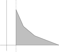
Figure 23.

Let ${\mathcal{I}}$ be an ideal of finite codimension in ${\mathbb{C}}[[x,y]]$. It is proven in [4][8] that

$$e({\mathcal{I}})=2m({\mathcal{I}})$$

if and only if ${\mathcal{I}}$ is non degenerate, and that $e({\mathcal{I}})>2m({\mathcal{I}})$ otherwise.

Example 2 (continued). Looking at the Newton polygon of the ideal ${\mathcal{I}}$ we see that $e({\mathcal{I}})=2m({\mathcal{I}})=18$. This is confirmed by Theorem 5.16, saying that $e({\mathcal{I}})=12+6=18$.

We can compute $e({\mathcal{I}})$ in general, using the area of the regions associated with the successive Newton polygons that appear in the Newton process. If ${\Sigma}_{i}=({\sigma}_{1},\cdots,{\sigma}_{i})$ is a sequence of Newton maps, then ${\mathcal{I}}_{{\Sigma}_{i}}$ has a Newton polygon as before and $m({\mathcal{I}}_{{\Sigma}_{i}})$ is well defined.

Theorem 5.18.

Let ${\mathcal{I}}$ be a non-trivial ideal in ${\mathbb{C}}[[x,y]]$ of finite codimension and of depth $d$. Then

$$e({\mathcal{I}})=2\,\left(m({\mathcal{I}})+\sum_{i=2}^{d}\sum_{{\Sigma}_{i}}m({\mathcal{I}}_{{\Sigma}_{i}})\right),$$

the second summation being taken over all possible sequences of Newton maps of length $i$.

In order to prove the theorem, we consider first two lemma’s.

Lemma 5.19.

Let $\Delta$ be a Newton diagram such that ${\mathbb{R}}_{+}^{2}\setminus\Delta$ is bounded. Let $m(\Delta)$ be the area of ${\mathbb{R}}_{+}^{2}\setminus\Delta$. For each face $S$ of $\mathcal{N}(\Delta)$ with equation $p_{S}{\alpha}+q_{S}{\beta}=N_{S}$, denote by $\delta_{S}$ the number of points with integral coordinates on $S$. Then

$$2m(\Delta)=\sum_{S\subset\mathcal{N}(\Delta)}N_{S}(\delta_{S}-1).$$

Proof.

Let $S$ be a face of $\mathcal{N}(\Delta)$. Denote by $A_{1}=(x_{1},y_{1})$ and $A_{2}=(x_{2},y_{2})$ the origin and end of $S$, respectively. Denote by $m(S)$ the area of the region limited by the triangle $(A_{1},0,A_{2})$. Then

$$2m(S)=x_{2}y_{1}-x_{1}y_{2}=(x_{2}-x_{1})y_{1}+x_{1}(y_{1}-y_{2}).$$

Since $x_{2}-x_{1}=q_{S}(\delta_{S}-1)$ and $y_{1}-y_{2}=p_{S}(\delta_{S}-1)$, we conclude that

$$2m(S)=(q_{S}y_{1}+p_{S}x_{1})(\delta_{S}-1)=N_{S}(\delta_{S}-1).$$

Obviously $m(\Delta)$ is the sum of these areas $m(S)$. ∎

If in Lemma 5.19 the depth of ${\mathcal{I}}$ is one, then all faces $S$ are dicritical and $\delta_{S}-1=d_{S}$.

Lemma 5.20.

Let ${\Sigma}$ be a sequence of Newton maps and ${\mathcal{I}}_{{\Sigma}}$ the corresponding ideal. Assume that its Newton polygon has its origin on the line $x=N$. For each face $S$ of $\mathcal{N}({\mathcal{I}}_{{\Sigma}})$ with equation $p_{S}{\alpha}+q_{S}{\beta}=N_{S}$, denote by $\delta_{S}$ the number of points with integral coordinates on $S$. Then

$$2m({\mathcal{I}}_{{\Sigma}})=\sum_{S\subset\mathcal{N}({\mathcal{I}}_{{\Sigma}})}(N_{S}-Np_{S})(\delta_{S}-1).$$

Proof.

Let $S$ be a face of the Newton polygon of ${\mathcal{I}}_{{\Sigma}}$ with origin $A_{1}=(x_{1},y_{1})$ and end $A_{2}=(x_{2},y_{2})$. Denote by $m(S)$ the area of the region limited by the triangle $(A_{1},(N,0),A_{2})$. Then

$$2m(S)=(x_{2}-N)y_{1}-(x_{1}-N)y_{2}=(x_{2}-x_{1})y_{1}+x_{1}(y_{1}-y_{2})-N(y_{1}-y_{2}).$$

Since $x_{2}-x_{1}=q_{S}(\delta_{S}-1)$ and $y_{1}-y_{2}=p_{S}(\delta_{S}-1)$, we see that

$$2m(S_{v})=(q_{S}y_{1}+p_{S}x_{1}-Np_{S})(\delta_{S}-1)=(N_{S}-Np_{S})(\delta_{S}-1),$$

and $m({\mathcal{I}}_{{\Sigma}})$ is the sum of the areas $m(S)$. ∎

Now we can prove Theorem 5.18.

Proof.

We have by Lemma 5.19 that

$$2m({\mathcal{I}})=\sum_{v}N_{v}(\delta_{v}-1),$$

where $v$ runs over the vertices of the graph associated with ${\mathcal{N}}({\mathcal{I}})$. Here each vertex $v$ corresponds to a face $S_{v}$ whose supporting line has equation $p_{v}{\alpha}+q_{v}{\beta}=N_{v}$, and we set $\delta_{v}=\delta_{S_{v}}$.

Let ${\sigma}_{v}={\sigma}_{(p_{v},q_{v},\mu_{i})}$ be a Newton map associated with $S_{v}$, where $\mu_{i}$ is a root of the face polynomial $F_{{\mathcal{I}},S_{v}}$. We have by Lemma 5.20 that

$$2m({\mathcal{I}}_{{\sigma}_{v}})=\sum_{v_{i}}(N_{v_{i}}-N_{v}p_{v_{i}})(\delta_{v_{i}}-1),$$

where the sum is taken over the vertices $v_{i}$ of the graph associated with the Newton diagram of ${\mathcal{I}}_{{\sigma}}$. We have

$$\delta_{v}-1=d_{v}+\deg F_{{\mathcal{I}},S_{v}}$$

and

$$\deg F_{{\mathcal{I}},S_{v}}=\sum_{v^{\prime}}p_{v^{\prime}}(\delta_{v^{\prime}}-1),$$

where now the sum is over all vertices $v^{\prime}$ of the graphs associated with the Newton diagrams of the ${\mathcal{I}}_{{\sigma}}$ for all roots of $F_{{\mathcal{I}},S_{v}}$. For the last equality we use that ${\mathcal{I}}$ is of finite codimension. Then

$$\sum_{v^{\prime}}p_{v^{\prime}}(\delta_{v^{\prime}}-1)=\delta_{v}-1-d_{v}$$

and hence

$$2m({\mathcal{I}})+\sum_{v}\sum_{\sigma}2m({\mathcal{I}}_{{\sigma}_{v}})=\sum_{v}N_{v}d_{v}+\sum_{v}\sum_{v^{\prime}}N_{v^{\prime}}(\delta_{v^{\prime}}-1).$$

Continuing the same procedure we arrive at the formula

$$2\left(m({\mathcal{I}})+\sum_{i=2}^{d}\sum_{{\Sigma}_{i}}m({\mathcal{I}}_{{\Sigma}_{i}})\right)=\sum_{w}N_{w}d_{w},$$

where, on the right hand side, $w$ runs over all vertices of the Newton tree of ${\mathcal{I}}$. Since $d_{w}\neq 0$ if and only if $w$ is dicritical, we obtain the stated formula for $e({\mathcal{I}})$. ∎

Example 3 (continued). Looking at the Newton polygons arising in the Newton process for the ideal ${\mathcal{I}}$ we calculate $e({\mathcal{I}})=88+4+2+1+1+1+1+1+1+2=102$.

5.6. Łojasiewicz exponent

Definition 5.21.

Let ${\mathcal{I}}=(f_{1},\cdots,f_{r})$ be an ideal in ${\mathbb{C}}[[x,y]]$ of finite codimension. The Łojasiewicz exponent of ${\mathcal{I}}$, denoted by ${\mathcal{L}}_{0}({\mathcal{I}})$, is the infimum of ${\alpha}>0$ such that there exists an open neighbourhood $U$ of $0$ in ${\mathbb{C}}^{2}$ and a constant $c>0$ such that

$$\|x\|^{{\alpha}}\leq c\sup_{1\leq i\leq r}|f_{i}(x)|$$

for all $x\in U$.

By [9], we have that

$${\mathcal{L}}_{0}({\mathcal{I}})=\min\{r/s\mid(x,y)^{r}\subseteq\overline{{\mathcal{I}}^{s}}\},$$

and

$${\mathcal{L}}_{0}({\mathcal{I}})=\sup_{{\gamma}\in\mathcal{T}}\frac{\inf_{h\in{\mathcal{I}}}\text{ord}(h\circ{\gamma})}{\text{ord}({\gamma})},$$

where $\mathcal{T}$ denotes the set of analytic maps $({\mathbb{C}},0)\to({\mathbb{C}}^{2},0)$. The number on the right hand side of the previous equality is called the order of contact of ${\mathcal{I}}$ in [10]. They proved that, if

$$f_{a}=\prod_{b}f_{a,b}^{n_{a,b}}$$

is the decomposition of $f_{a},1\leq a\leq r,$ into irreducible components in ${\mathbb{C}}[[x,y]]$, then

(5.1) $${\mathcal{L}}_{0}({\mathcal{I}})=\max_{a,b}\frac{\min_{i}\text{ord}(f_{i}\circ{\gamma}_{a,b})}{\text{ord}({\gamma}_{a,b})},$$

where ${\gamma}_{a,b}$ is a parametrization of $\{f_{a,b}=0\}$.

Proposition 5.22.

Let ${\mathcal{I}}$ be an ideal in ${\mathbb{C}}[[x,y]]$ of finite codimension. Then

$${\mathcal{L}}_{0}({\mathcal{I}})=\max_{v\in{\mathcal{D}}({\mathcal{I}})}\frac{N_{v}}{\rho(v)},$$

where $\rho(v)$ is as in Definition 5.7.

Proof.

We note that ${\mathcal{L}}_{0}({\mathcal{I}})={\mathcal{L}}_{0}(\overline{{\mathcal{I}}})$. Let $g_{{\lambda}},g_{\mu}$ be two sufficiently generic elements of ${\mathcal{I}}$ such that $e({\mathcal{I}})=e((g_{{\lambda}},g_{\mu}))$. Then $\overline{{\mathcal{I}}}=\overline{(g_{{\lambda}},g_{\mu})}$ and

$${\mathcal{L}}_{0}({\mathcal{I}})={\mathcal{L}}_{0}(\overline{{\mathcal{I}}})={\mathcal{L}}_{0}(\overline{(g_{{\lambda}},g_{\mu})})={\mathcal{L}}_{0}((g_{{\lambda}},g_{\mu})).$$

Now we can apply (5.1) and previous results on multiplicity and intersection multiplicity, more precisely Remark 5.1, Corollary 5.4 and Proposition 5.9. ∎

Example 7. We consider an example in [10]. Let

$$f_{s}=sx+x^{3}+y^{8},\quad g=x^{2}-y^{101},$$

and ${\mathcal{I}}_{s}=(f_{s},g)$. If $s\neq 0$, the Newton tree of ${\mathcal{I}}_{s}$ is the tree on the left in Figure 24, and for $s=0$ it is the one on the right. Then we can compute that ${\mathcal{L}}_{0}({\mathcal{I}}_{s})=16$ if $s\neq 0$, and that ${\mathcal{L}}_{0}({\mathcal{I}}_{0})=8$.

Figure 24.

Remark 5.23.

We note that in the previous example we have $e({\mathcal{I}}_{s})=e({\mathcal{I}}_{0})=16$. It is proven in [11] that in an $e$-constant family of ideals, the Łojasiewicz exponent is lower semi-continuous. It is not the case in general.

6. Geometric version

Our Newton algorithm in section 2 was developed from an algebraic point of view; we did not include coordinate changes. This is in particular useful in studying when two ideals have the same integral closure.

From geometric point of view however, our Newton tree/process is sometimes not minimal. Consider for example the principal ideal ${\mathcal{I}}$ in ${\mathbb{C}}[[x,y]]$ generated by $(y+x^{2}+x^{3})^{2}+x^{7}$. Its Newton algorithm consists of three Newton maps $\sigma_{1}$, $\sigma_{2}$ and $\sigma_{3}$, given by

$$\begin{cases}x=x_{1}\\ y=x_{1}^{2}(y_{1}-1)\end{cases}\qquad\begin{cases}x_{1}=x_{2}\\ y_{1}=x_{2}(y_{2}-1)\end{cases}\text{and}\qquad\begin{cases}x_{2}=x_{3}^{2}\\ y_{2}=x_{3}(y_{3}-1),\end{cases}$$

respectively, resulting in the ideal $(x_{3}^{14}y_{3})$.

If on the other hand we would perform first the change of coordinates $(x,y)\to(x,y-x^{2}-x^{3})$ in ${\mathbb{C}}[[x,y]]$, the given ideal would be generated by $y^{2}+x^{7}$. And then the Newton map $\sigma$ given by $x=x_{1}^{2},y=x_{1}^{7}(y_{1}-1)$ immediately leads to the ideal $(x_{1}^{14}y_{1})$. We could say that the ‘algebraic depth’ of ${\mathcal{I}}$ is $3$ and its ‘geometric depth’ is $1$.

In a sequel to this paper, we will develop a geometric version, using Newton maps and appropriate coordinate changes, yielding ‘minimal’ Newton trees with geometric interpretation. In particular their vertices will correspond to exceptional components of the so-called relative log canonical model of the blow-up of $\operatorname{Spec}{\mathbb{C}}[[x,y]]$ in ${\mathcal{I}}$. In Example 3 for instance, this ‘minimal’ Newton tree has only six vertices: the four dicritical ones and those with decorations $N=22$ and $N=46$.

References

- [1] E. Artal, P. Cassou-Noguès, I. Luengo, A. Melle Hernández Quasi-ordinary power series and their zeta functions, Mem. Amer. Math. Soc. 178 (2005), vi+85.
- [2] E. Artal, P. Cassou-Noguès, I. Luengo, A. Melle Hernández -Quasi-ordinary power series: factorisation, Newton trees and resultants, Topology of algebraic verieties and singularities, Contemp. Math. 538 (2011), 321-343.
- [3] C. Bivia-Ausina Joint reductions of monomial ideals and multiplicity of complex analytic maps, Math. Res. Lett. 15 (2008), 389-407.
- [4] C. Bivia-Ausina, T. Fukui, M. Saia Newton filtrations, graded algebras and codimension of non-degenerate ideals, Math. Proc. Camb. Soc. 133 (2002), 55-75.
- [5] R. Debremaeker and V. Van Lierde The effect of quadratic transformations on degree functions, Contributions to Algebra and Geometry 47 (2006), 121-135.
- [6] D. Eisenbud and W. Neumann Three dimensional link theory and invariants of plane curve singularities, Annals of Mathematics Studies 110 (1986), Princeton University Press.
- [7] D. Katz and J. Validashti Multiplicities and Rees valuations, Collect. Math. 61 (2010), 1-24.
- [8] A.Kouchnirenko Polyhèdres de Newton et nombres de Milnor, Invent. Math. 32 (1976), 1-31.
- [9] M.Lejeune-Jalabert, B.Teissier Cloture intégrale des idéaux et équisingularité, Ann. Fac. Sci. Toulouse Math. 17 (2008), 781-859.
- [10] J.D. McNeal and A. Némethi The order of contact of a holomorphic ideal in , Math. Z. 250 (2005), 873-883.
- [11] A. Ploski Semicontinuity of the Lojasiewicz exponent, ArXiv 1102.4730.
- [12] D. Rees Generalizations of reductions and mixed multiplicities, J. Lond. Math. Soc. 29 (1984), 397-414.
- [13] D. Rees and R. Sharp On a theorem of B. Teissier on multiplicities of ideals in local rings, J. Lond. Math. Soc. 18 (1978), 449-463.
- [14] I. Swanson and C. Huneke Integral closure of ideals, rings, and modules, Lond. Math. Soc. L.N.S. 336 (2006).
- [15] M. Saia The integral closure of ideals and the Newton filtration, J. Algebraic Geometry 5 (1996), 1-11.
- [16] L. Van Proeyen and W. Veys The monodromy conjecture for zeta functions associated to ideals in dimension two, Ann. Inst. Fourier 60 (2010), 1347-1362.
- [17] W. Veys and W. Zuniga-Galindo Zeta functions for analytic mappings, log-principalization of ideals, and Newton polyhedra, Trans. Amer. Math. Soc. 360 (2008), 2205-2227.
- [18] C.T.C Wall Singular points on plane curves, London Mathematical Society Student Texts 63 (2004), Cambridge University Press.