Spin transistor action from Onsager reciprocity and SU(2) gauge theory

Abstract

We construct a local gauge transformation to show how, in confined systems, a generic, weak nonhomogeneous $SU(2)$ spin-orbit Hamiltonian reduces to two $U(1)$ Hamiltonians for spinless fermions at opposite magnetic fields, to leading order in the spin-orbit strength. Using an Onsager relation, we further show how the resulting spin conductance vanishes in a two-terminal setup, and how it is turned on by either weakly breaking time-reversal symmetry or opening additional transport terminals. We numerically check our theory for mesoscopic cavities as well as Aharonov-Bohm rings.

Transistor action is often based on symmetries. To switch on and off a field effect transistor, an external gate turns a three-dimensional insulator into a two-dimensional metal and back. Compared to the off-state, the on-state has thus reduced dimensionality and symmetry. The relevance of symmetries in transistor action is even more pronounced in some recently proposed spin-based transistors, whose action follows directly from the breaking of spin rotational symmetry, by tuning spin-orbit interaction (SOI) around a special symmetry point sel , where the SOI field reduces to two identical $U(1)$ fields with opposite coupling constants duc10 .

In this manuscript, we propose a new class of spin transistors whose action is based on an Onsager reciprocity relation. We show that in confined quantum coherent systems with spatially inhomogeneous SOI (Rashba, Dresselhaus or impurity SOI, or a combination of the three), an appropriate $SU(2)$ gauge transformation allows to express the spin conductance $G_{ij}^{\uparrow}-G_{ij}^{\downarrow}$ between two terminals labeled $i$ and $j$ through the charge magnetoconductance $G_{ij}({\cal B})$ as $G_{ij}^{\uparrow}-G_{ij}^{\downarrow}=G_{ij}({\cal B})-G_{ij}(-{\cal B})$. This holds to leading order in the ratio $L/\ell_{\rm so}\ll 1$ of the system size $L$ and the spin-orbit (precession) length $\ell_{\rm so}$. The pseudo magnetic field ${\cal B}$ arises from the gauge-transformed SOI. Current conservation together with the Onsager relation $G_{ij}({\cal B})=G_{ji}(-{\cal B})$ Onsager ; Buttiker86 then forces $G_{ij}^{\uparrow}-G_{ij}^{\downarrow}=0$ to leading order for a two-terminal setup. This is the off state of our transistor. The on state is obtained by either opening additional terminals or breaking time-reversal symmetry with a true magnetic field $B_{0}$, in which case $G_{ij}^{\uparrow}-G_{ij}^{\downarrow}=G_{ij}(B_{0}+{\cal B})-G_{ij}(B_{0}-{\cal B})\neq 0$, even in a two-terminal setup. Our Onsager spin transistor can thus be controlled either electrically or magnetically. In both instances, this turns on a spin conductance $G_{ij}^{\uparrow}-G_{ij}^{\downarrow}\propto\ell_{\rm so}^{-1}$ with an on/off ratio $\propto(\ell_{\rm so}/L)^{2}\gg 1$. The mechanism works in diffusive as well as ballistic systems, and is more pronounced in regular systems with few channels.

Aleiner and Falko constructed a gauge transformation to show that, in confined systems with $L/\ell_{\rm so}\ll 1$, a homogeneous $k$-linear SOI has a much weaker effect on charge transport than the naive expectation $\propto\ell_{\rm so}^{-1}$ Aleiner . Brouwer and collaborators later argued that terms $\propto\ell_{\rm so}^{-1}$ in the charge conductance survive the gauge transformation for SOI with spatially varying strength Brouwer . The relevance of the pseudo magnetic field for a specific mesoscopic system with inhomogenous SOI was noticed in Ref. SU2 . It is however not clear how much of the gauge arguments of Refs. Aleiner ; Brouwer ; Tokatly carry over to spin transport in generic systems Ada10 . Below we show that gauge transformations result in different symmetries for charge and for spin transport comment-charge-cond .

Our starting point is a two-dimensional Hamiltonian for electrons with SOI, which we write as ($\hbar\equiv 1$)

$$H=-\frac{1}{2m}D_{\mu}D_{\mu}+V(\mathbf{x})\;.$$ (1)

Here, $V({\bf x})$ is a spin-diagonal potential and the covariant derivative $D_{\mu}=\partial_{\mu}-(ik_{\rm so}/2)\sigma^{a}A_{\mu}^{a}$ contains the SOI via the $SU(2)$ gauge field $\sigma^{a}A_{\mu}^{a}$, with the Pauli matrix $\sigma^{a}$. From here on, Latin indices are spin indices, while Greek letters denote spatial indices. The SOI constant $k_{\rm so}$ determines the spin-orbit length as $\ell_{\rm so}=\pi|k_{\rm so}|^{-1}$. We consider a gauge transformation ${\cal O}\rightarrow{\cal O}^{\prime}=U{\cal O}U^{-1}$ with $U=\exp(i{\sigma^{a}}{\Lambda}^{a}/2)\simeq 1+i\sigma^{a}\Lambda^{a}/2$, and search for a $\Lambda^{a}$ that reduces the leading order, $k_{\rm so}$-linear part of the SOI to a spin-diagonal $U(1)\times\sigma^{z}$ structure. We use the well-known decomposition ($\epsilon_{\mu\nu}$ is the totally antisymmetric tensor of order two) for each spin component

$$A_{\mu}^{a}=-(\partial_{\mu}\chi^{a}+\epsilon_{\mu\nu}\partial_{\nu}\phi^{a})\;,$$ (2)

with $\phi^{a}$ given by $\nabla^{2}\phi^{a}=\epsilon_{\mu\nu}\partial_{\mu}A_{\nu}^{a}$. In particular, $\phi^{a}$ is necessarily nonzero for spatially varying SOI. It is straightforward to see that the choice $\Lambda^{a}=k_{\rm so}\chi^{a}$ gauges away the gradient part of the $SU(2)$ vector potential to linear order in $k_{\rm so}$,

$$A_{\mu}^{a} \rightarrow (A^{\prime})_{\mu}^{a}=-\epsilon_{\mu\nu}\partial_{\nu}\phi^{a}+\mathcal{O}(k_{\rm so})\;.$$ (3)

Note that $\mathcal{O}(k_{\rm so})$ corrections in $A_{\mu}^{a}$ lead to $\mathcal{O}(k_{\rm so}^{2})$ corrections in the Hamiltonian. If the SOI strength is spatially constant, $\phi^{a}=0$ and one recovers the result of Ref. Aleiner that all ${\cal O}(k_{\rm so})$-terms are gauged away.

We next want to extract the leading order, linear in $k_{\rm so}\chi^{a}\ll 1$ dependence of transport properties such as conductances, and thus use

$${\cal O}^{\prime}=U{\cal O}U^{-1}={\cal O}+ik_{\rm so}[{\sigma^{a}}\chi^{a},{\cal O}]/2\;.$$ (4)

In particular we have $D_{\mu}\rightarrow D_{\mu}^{\prime}$ with

$$\sigma^{a}\rightarrow{\sigma^{a}}^{\prime}=\sigma^{a}+k_{\rm so}\epsilon^{abc}\chi^{b}({\bf x})\sigma^{c}\,.$$ (5)

To calculate spin conductances we need to gauge transform the operator for spin current through a cross-section $C_{j}$ in terminal $j$, $\hat{I}^{a}_{j}=\int_{C_{j}}d\alpha\,\{{\bf n}_{\alpha}\cdot{\bf j}(\alpha),\sigma^{a}\}$. We obtain

$$(\hat{I}^{\prime})^{a}_{j} = \int_{C_{j}}d\alpha\,\left[\{{\bf n}_{\alpha}\cdot{\bf j}^{\prime}(\alpha),\sigma^{a}+k_{\rm so}\,\epsilon^{abc}\chi^{b}(\alpha)\sigma^{c}\}\right]$$ (6)

$$= \hat{J}^{a}_{j}+k_{\rm so}\delta\hat{J}^{a}_{j}$$

where $\hat{J}^{a}_{j}$ is the “naive” spin current of the transformed Hamiltonian, not accounting for the rotation (5) of the spin axes. We further need the Heisenberg picture operators $\hat{I}^{a}_{j}(t)={\rm e}^{iHt}\hat{I}_{j}^{a}{\rm e}^{-iHt}$ which transform as

$$(\hat{I}^{\prime})^{a}_{j}(t) = \hat{J}^{a}_{j}(t)+k_{\rm so}\delta\hat{J}^{a}_{j0}(t)+{\cal O}(k_{\rm so}^{2})\,.$$ (7)

Here the subscript $0$ means that the time-evolution is through the $k_{\rm so}=0$ Hamiltonian.

Linear response relates chemical potentials in external reservoirs and currents in the leads via the spin-conductance matrix as $I_{i}^{a}=\sum_{j}G_{ij}^{a}\mu_{j}/e$. It is somehow tedious, though straightforward to show that, to linear order in $k_{\rm so}$, the gauge transformation gives $G_{ij}^{a}\rightarrow(G^{\prime}_{ij})^{a}$, with the conductance matrix $(G^{\prime}_{ij})^{a}$ evaluated in the same way as $G_{ij}^{a}$ but with the spin current operators $\hat{J}^{a}_{j}$ of the transformed Hamiltonian in Eq. (7). Thus, to leading order in $k_{\rm so}$, infinitesimal nonabelian gauge transformations preserve the form of the spin conductance. Note that global gauge transformations (i.e. global spin rotations), whether infinitesimal or finite, are easy to introduce via the corresponding rotation matrix ${\cal R}$ as $G_{ij}^{a}={\cal R}^{ab}(G_{ij}^{\prime})^{b}$. All global or local spin gauge transformations leave the potential $V({\bf x})$ invariant.

We are now equipped to use the gauge transformation to explore the spin conductance. We first focus on the exactly solvable case of a Rashba SOI rashba with a spatially varying strength $\alpha({\bf x})=k_{\rm so}\,\overline{\alpha}\,({\bf x}\cdot\mathbf{f})$, with a dimensionless function $\overline{\alpha}$, whose gradient always points in the direction of the unit vector $\mathbf{f}$. One has $A_{\mu}^{a}=-2\overline{\alpha}(\mathbf{x}\cdot\mathbf{f})\epsilon_{a\mu}$, $\phi^{a}(\mathbf{x})=\varphi(\mathbf{x})f^{a}$, and Eq. (3) gives

$$(A^{\prime})_{\mu}^{a} = -\epsilon_{\mu\nu}\partial_{\nu}\varphi(\mathbf{x})f^{a}+\mathcal{O}(k_{\rm so})\;,$$ (8a)

$$D_{\mu}^{\prime} = \partial_{\mu}+\frac{i}{2}k_{\rm so}\epsilon_{\mu\nu}\partial_{\nu}\varphi(\mathbf{x}){\bm{\sigma\cdot}}\mathbf{f.}$$ (8b)

After the global spin rotation ${\bm{\sigma\cdot}}\mathbf{f\rightarrow}\sigma^{z}$, Eq. (1) becomes

$$H = \left(\begin{array}[]{cc}h(\bm{a})&0\\ 0&h(-\bm{a})\end{array}\right)+{\cal O}(k_{\rm so}^{2})\;,$$ (9c)

$$h(\bm{a}) = -\frac{1}{2m}\left[\nabla+ik_{\rm so}\bm{a}(\mathbf{x})\right]^{2}+V(\mathbf{x})\;.$$ (9d)

Thus to linear order in $k_{\rm so}$, the Hamiltonian is mapped onto a block spin Hamiltonian where the opposite spins feel opposite, purely orbital pseudo magnetic fields ${\mathcal{B}}=(\nabla\times\bm{a})_{z}$ generated by the $U(1)$ vector potential $a_{\mu}=\frac{1}{2}\epsilon_{\mu\nu}\partial_{\nu}\varphi(\mathbf{x})$. We obtain $\mathcal{B}(\mathbf{x})=k_{\rm so}\mathbf{f}\cdot\nabla\bar{\alpha}$. Transforming back to the original gauge, the spin conductance is obtained as $G_{ij}^{a}=\big{[}G_{ij}(\mathcal{B})-G_{ij}(-\mathcal{B})\big{]}f^{a}+{\cal O}(k_{\rm so}^{2}).$ In this simple example, the spin conductance is thus the difference of two charge conductances $G_{ij}$ at opposite pseudo magnetic fields. For generally varying SOI, one cannot choose a spin quantization axis as before. Thus we need to define one pseudo-magnetic field per spin polarization, i.e. we define ${\cal B}_{a}=\partial_{x}A_{y}^{a}-\partial_{y}A_{x}^{a}$ as the magnitude of a pseudo magnetic field (pointing always in $z$-direction) that arises solely from the $a$ component of $\phi^{a}$. To linear order in $k_{\rm so}L$, the superposition principle gives the spin conductance along axis $a$ as solely due to the component of $\phi^{a}$, $G_{ij}^{a}=G_{ij}({\cal B}_{a})-G_{ij}(-{\cal B}_{a})$. The same argument gives the leading-order spin conductance in the presence of an externally applied (i.e. true) magnetic field $B_{0}$ as

$$G_{ij}^{a}(B_{0})=G_{ij}(B_{0}+{\cal B}_{a})-G_{ij}(B_{0}-{\cal B}_{a})+{\cal O}(k_{\rm so}^{2}).$$ (10)

This is our main result. It expresses the spin conductance of the original dot with SOI in terms of charge conductances of the dot without SOI, but with effective magnetic fields $B_{0}\pm{\cal B}_{a}$ arising from the true applied field, $B_{0}$, and the pseudo field, ${\cal B}_{a}$, generated by the gauge transformation and the SOI.

The key observation is then that the reciprocity relation $G_{ij}(B)=G_{ji}(-B)$ Buttiker86 , together with gauge invariance, $\sum_{j}G_{ij}(B)=0$, imply that the spin conductance (10) vanishes to order $\mathcal{O}(k_{\rm so})$ in two-terminal geometries in the absence of external magnetic field, since only then $G_{ij}(-{\cal B}_{a})\!=\!G_{ji}({\cal B}_{a})\!=\!G_{ij}({\cal B}_{a})$. On the contrary, $G_{ij}^{a}$ is linear in $k_{\rm so}$, i.e. much larger, when an external magnetic field is applied or when one (or more) additional terminals are open. Thus, multi-terminal spin conductances linearly depend on $k_{\rm so}L$, whereas two-terminal local conductances are quadratic or higher order in $k_{\rm so}L$. These restrictions imply that any coherent conductor with spatially varying SOI can be operated as a spin transistor, whose action is controlled by either opening an extra terminal or applying an external magnetic field. This is the fundamental mechanism on which the Onsager spin transistor we propose is based.

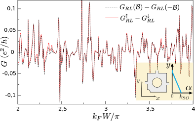
Figure 1: Comparison of the spin conductance $G_{RL}^{y}\!=\!G^{\uparrow}_{RL}\!-\!G^{\downarrow}_{RL}$ with the difference in the magnetoconductance, Eq. (10), for transport (from left to right lead) through the three-terminal ballistic quantum dot (see inset) with linear size $L$, leads of width $W$ and spatially varying SOI $\alpha({\bf x})\!=\!k_{\rm so}\bar{\alpha}({\bf x})=k_{\rm so}(y/L)$ (i.e. ${\cal B}\!=\!\partial_{y}\alpha\!=\!k_{\rm so}/L$) with $k_{\rm so}L\approx 0.3$.

We numerically confirm these results by computing Wimmer09 the charge and spin conductances for two- and three-terminal mesoscopic cavities and rings (sketched in the inset of Figs. 1–3). We first assume a Rashba SOI with constant gradient over the whole conductor, $\alpha({\bf x})\!=\!(y/L)k_{\rm so}$, and check the prediction (10) that the spin conductance can be expressed in terms of the charge conductance of the transformed system without SOI but with a magnetic field ${\cal B}$. In Fig. 1, the spin conductance $G^{y}_{RL}\!=\!G^{\uparrow}_{RL}-G^{\downarrow}_{RL}$ (from now on the $y$-axis is the spin quantization axis) in the absence of magnetic field is compared to the difference of the charge conductance, $G_{RL}({\cal B})\!-\!G_{RL}(-{\cal B})$ in the absence of SOI, but with magnetic field ${\cal B}=\partial_{y}\alpha$. Both quantities exhibit precisely the same mesoscopic conductance fluctuations as a function of Fermi momentum, as predicted by Eq. (10). We found that this level of agreement holds up to $k_{\rm so}L\approx 1$, beyond which terms quadratic and higher order in $k_{\rm so}$ are no longer subdominant.

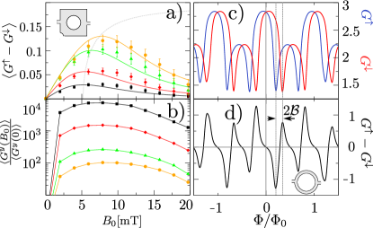
Figure 2: Spin conductances for two-terminal geometries as a function of an applied magnetic field $B_{0}$. (a) Average spin conductance of a chaotic cavity (inset) for four different strengths of a linearly varying SOI (same as inset Fig. 1) with $k_{\rm so}L\approx 0.16,0.33,0.67$ and 1.0 from bottom to top curve. Symbols with statistical errorbars mark numerical results for the average spin conductance, full lines depict the theoretical prediction (11). The grey dashed line shows predicted spin conductance maxima (from Eq. (11)) for varying gauge field. (b) corresponding on-to-off ratios $\left\langle G^{y}(B_{0})\right\rangle/\left\langle G^{y}(0)\right\rangle$. (c) spin resolved conductances $G^{\uparrow(\downarrow)}(\Phi)$ for an AB ring (inset panel (d)) as a function of flux $\Phi\!=\!\pi R^{2}B_{0}$, showing a shift $\pm{\cal B}$ due to the gauge field ${\cal B}=\nabla\alpha$ arising from SOI $\alpha\!=\!(y/L)k_{\rm so}$ with $k_{\rm so}L\!=\!1$. (d) resulting spin conductance $G^{y}(\Phi)$ of a single AB ring. Inset panel (a): Sinai-type billard: linear size $L$, stopper disk with radius $R_{i}=L/10$, leads of width $W=L/15$ hosting 4 transverse channels. Inset panel (d): AB ring: radius $R=L/2$, width $W=L/15$ with 4 open channels.

For weak magnetic fields (with an associated cyclotron radius larger than $L$), $G_{ij}(B)-G_{ij}(-B)$ is predominantly given by quantum coherent contributions only. They give rise, on top of the mesoscopic fluctuations displayed in Fig. 1, to a shift $\delta G$ in the (energy) averaged conductance, known as weak localization correction. In the presence of a magnetic field, $\delta G$ exhibits a damping that is Lorentzian-like, $\delta G(B)=\delta G(0)/(1+\xi B^{2})$, for chaotic ballistic cavities Bar93 with $\delta G(0)\sim(1/4)e^{2}/h$ and $\xi$ proportional to the dwell time in the cavity. According to the prediction (10) for the two-terminal case, the presence of an external magnetic field $B_{0}$ leads to a finite spin conductance $G^{y}(B_{0})=G(B_{0}+{\cal B})-G(B_{0}-{\cal B})$, with ${\cal B}=\partial_{y}\alpha$. Then its energy average is

$$\langle G^{y}(B_{0})\rangle=\frac{\delta G(0)}{1+\xi(B_{0}+{\cal B})^{2}}-\frac{\delta G(0)}{1+\xi(B_{0}-{\cal B})^{2}}\,.$$ (11)

This line of reasoning is confirmed in Fig. 2(a) where numerically calculated spin conductances (symbols) for the chaotic cavity with linearly varying SOI are compared to the prediction (11) (full lines). Figure  2(b) shows the corresponding on-off ratios $\langle G^{y}(B_{0})\rangle/\langle G^{y}(0)\rangle$.

Alternatively, we consider few-channel regular Aharonov-Bohm (AB) rings where $k_{\rm so}$-linear spin currents can be turned on by a magnetic flux SU2 . These systems exhibit large almost periodic AB conductance oscillations instead of the weaker, randomly-looking conductance fluctuations. In Fig. 2(c) we present numerically computed spin resolved conductances $G^{\uparrow(\downarrow)}(\Phi)$ as a function of flux $\Phi=\pi R^{2}B_{0}$ (in units of the flux quantum $\Phi_{0}=h/e$) for an AB ring (inset panel (d)) in presence of the same linearly varying SOI as for the cavity. As expected, the conductance traces for the spin-up and -down channels are shifted against each other by $\pm{\cal B}\!=\!\pm\partial_{y}\alpha$. This shift gives rise to a finite $B_{0}$-periodic spin conductance $G^{y}\!=\!G^{\uparrow}\!-\!G^{\downarrow}$ as displayed in Fig. 2(d). At $B_{0}\!=\!0$, first order spin conductance is forbidden by the Onsager relation. $G^{y}$ vanishes further for fields corresponding to $\Phi_{0},\Phi_{0}/2$ and $\Phi_{0}/4$, where maxima and minima of the usual charge magnetoconductance occur. Maxima of $G^{y}$ appear at points where the shifted spin resolved $G^{\uparrow(\downarrow)}$ have their minima. This holds for regular, or quasi-regular electronic dynamics which requires clean AB rings with few-channels. Of particular interest in the AB case are: (i) the magnitude of the spin conductance, which exceeds its value in chaotic systems by one to two orders of magnitude (compare the vertical axes scales in Fig. 1 and 2(d)), and (ii) the control one has over the spin conductance: Applying an integer or half-integer flux quantum gives the off state of our transistor, while the on state is recovered at $B_{0}\!=\!\pm[(\Phi_{0}/4)/(\pi R^{2})\!-\!{\cal B}]$. The on/off spin current ratio can be made arbitrarily large, as it exactly vanishes in the off state.

As said above, $k_{\rm so}$-linear spin conductances can also be turned on by adding an additional terminal. As shown in Fig. 3(a,b) we find a difference of at least three orders of magnitude in spin conductance, $G^{y}_{\rm 2T}$ vs. $G^{y}_{\rm 3T}$, for two- and three-terminal rings. In panel (c) a double log representation of the data from (b) reveal the cubic vs. linear $k_{\rm so}L$ dependence of $G^{y}_{\rm 2T}$ (top symbol sequence in (c)) and $G^{y}_{\rm 3T}$ (third sequence from top) in line with our predictions.

So far we have considered linearly varying SOI. However, our theory holds generally and works well also for more generic spatial dependence of the SOI. We confirm this by calculating $G^{y}(k_{\rm so}L)$ for a ring with SOI $\alpha(\mathbf{r})=k_{\rm so}\cos^{2}(2\pi x/L_{1})\cos^{2}(2\pi y/L_{2})$ with $L/L_{1}\!=\!15,L/L_{2}\!=\!6$ giving rise to SOI bumps on scales of the ring width. As demonstrated in Fig. 3(c) we recover again the linear vs. cubic scaling with $k_{\rm so}L$ for the two- and three-terminal setting (second and fourth symbol sequence from top), in full accordance with our theory.

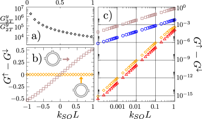
Figure 3: Onsager symmetry-based transistor action resulting from the difference in spin conductance of two- and three-terminal mesoscopic rings (insets panel (b)). (a) On–off ratio and (b) separate spin conductances $G^{y}_{\rm 3T}$ and $G^{y}_{\rm 2T}$ for AB ring in three- and two-terminal mode as a function of a spatially nonuniform SOI, $\alpha=(y/L)k_{\rm so}$. (c) double-log plot of same data as in (b) (top and third symbol sequence) and of corresponding $G^{y}_{\rm 3T}$ and $G^{y}_{\rm 2T}$ (second and fourth sequence) for a more generic nonuniform SOI $\alpha=k_{\rm so}\cos^{2}(2\pi x/L_{1})\cos^{2}(2\pi y/L_{2})$.

We conclude with a few remarks:

(i) Mesoscopic rings based on InAs Berg06 or p-doped GaAs samples which are known to exhibit large and tunable SOI ensslin are excellent candidates to experimentally probe our theory. Inhomogeneous SOI could, e.g., be realized through a top gate covering only part of the system. Additionally, a measurement protocol for spin currents based on symmetries of charge transport through quantum point contacts Stano could be implemented.

(ii) Inhomogeneous SOI is also a prerequisite for various specific proposals for spin splitting Kho04 ; Sun05 and analogues of the Stern-Gerlach effect Ohe05 . Our theory provides a rather general, common footing to interpret them. For instance, the Stern-Gerlach based spin separation, usually explained in terms of a Zeeman coupling in a non-uniform (in-plane) magnetic field (associated with Rashba SOI), finds its explanation in the opposite bending of electron paths owing to the Lorentz force associated with our gauge field $\pm{\cal B}$.

(iii) Another gauge transformation, dual to ours, allows to transform a nonuniform Zeeman term into two decoupled components with an additional gauge field Kor77 .

(iv) While the spin conductance fluctuations are similar in a (phase coherent) diffusive system, its classical magnetoconductance has a linear in magnetic field contribution originating from the classical Hall effect. Thus in a diffusive system with inhomogeneous SOI, we expect a spin conductance with a nonzero average value proportional to the classical Hall conductance. This spin conductance can be estimated Ada-et-al as $\langle G^{a}\rangle\sim(e^{2}/h)(k_{\rm so}\ell)$ where $\ell$ is the mean free path. We stress that $\langle G^{a}\rangle$ is based on a classical effect in that it is robust against effects such as dephasing and temperature broadening.

We thank M. Duckheim for carefully reading our manuscript, and D. Loss, J. Nitta and M. Wimmer for helpful conversations. This work was supported by TUBITAK under grant 110T841 and the funds of the Erdal İnönü chair (IA), by NSF under grant DMR-0706319 and the Swiss Center for Excellence MANEP (PJ), and by DFG within SFB 689 (MS,KR).

References

- (1) J. Schliemann, J.C. Egues, and D. Loss, Phys. Rev. Lett. 90, 146801 (2003).
- (2) M. Duckheim et al., Phys. Rev. B 81, 085303 (2010).
- (3) L. Onsager, Phys. Rev. 38, 2265 (1931).
- (4) M. Büttiker, Phys. Rev. Lett. 57, 1761 (1986).
- (5) I.L. Aleiner and V.I. Fal’ko, Phys. Rev. Lett. 87, 256801 (2001).
- (6) P. W. Brouwer, J. N. H. J. Cremers, and B. I. Halperin, Phys. Rev. B 65, 081302 (2002).
- (7) Y. Tserkovnyak and A. Brataas, Phys. Rev. B 76, 155326 (2007).
- (8) For a comprehensive recent account see: I.V. Tokatly and E. Ya. Sherman, Ann. Phys. 325, 1104 (2010).
- (9) To give but one example, a nonuniversal behavior of spin currents has been pointed out for systems with universal charge current characteristics in: İ. Adagideli et al., Phys. Rev. Lett. 105, 246807 (2010).
- (10) Our gauge transformation gives for the charge conductance, which is a linear function of , in agreement with Ref. Brouwer , regardless of the geometry.
- (11) E.I. Rashba, Sov. Phys. Solid State 2, 1109 (1960).
- (12) The transport calculations are performed using a recursive Green’s function technique, see: M. Wimmer and K. Richter, J. Comp. Phys. 228, 8548 (2009).
- (13) H.U. Baranger, R.A. Jalabert, and A.D. Stone, Phys. Rev. Lett. 70, 3876 (1993).
- (14) T. Bergsten, T. Kobayashi, Y. Sekine, and J. Nitta, Phys. Rev. Lett. 97, 196803 (2006).
- (15) B. Grbić et al., Phys. Rev. Lett. 99, 176803 (2007).
- (16) P. Stano and Ph. Jacquod, Phys. Rev. Lett. 106, 206602 (2011).
- (17) M. Khodus, A. Shekhter, and A.M. Finkel’stein, Phys. Rev. Lett. 92, 086602 (2004).
- (18) Q.-F. Sun and X.C. Xie, Phys. Rev. B 71, 155321 (2005).
- (19) J.-I. Ohe, M. Yamamoto, T. Ohtsuki, and J. Nitta, Phys. Rev. B 72, 041308 (2005).
- (20) V. Korenman, J.L. Murray, and R.E. Prange, Phys. Rev. B 16, 4032 (1977).
- (21) İ. Adagideli et al., unpublished.