Symmetry Energy and Universality classes of holographic QCD

Abstract:

We study nuclear symmetry energy of dense matter using holographic QCD. We calculate it in a various holographic QCD models and show that the scaling index of the symmetry energy in dense medium is almost invariant under the smooth deformation of the metric as well as the embedding shape of the probe brane. We find that the scaling index depends only on the dimensionality of the branes and space-time. Therefore the scaling index of the symmetry energy characterizes the universality classes of holographic QCD models. We suggest that the scaling index might be also related to the non-fermi liquid behavior of the interacting nucleons.

1 Introduction

Nuclear symmetry energy is one of key words in nuclear physics as well as in astrophysics. Its density dependence is a core quantity of asymmetric nuclear matter which has important effects on heavy nuclei and is essential to understand neutron star properties. A big surprise is that such an important quantity is still poorly understood after 80 years of its definition, especially in the supra-saturation density regime. See references [1, 2, 3, 4, 5, 6, 7, 8, 9] for a review and for a recent discussion. Not much data is available from experimental side and theoretical calculations showed all possible results in high density such that no consensus could be reached: some showed stiff dependence on density, while others showed soft one depending on models and parameters.

Given this situation, it would be very interesting if we can examine the behavior of the nuclear symmetry energy at high densities with a reliable calculational tool. Recently [10] we used a gauge/gravity duality [11, 12, 13, 14, 15] to calculate the nuclear symmetry energy. We treated the dense matter in confined phase using the method developed in our previous paper [16, 17]. Our result showed that the symmetry energy should be stiff in high density and its density dependence goes like $\sim\rho^{1/2}$. There, we attributed the stiffness to the repulsion due to the Pauli principle and suggested the relation of the scaling exponent to the anomalous dispersion relation.

The purpose of this paper is to examine how universal or robust is the result. If the result changes under small variation of the gluon dynamics, the result is not very interesting since the true QCD dual is not yet known. Only when the result is largely background independent, it can be considered as an interesting one. The universality of the $\eta/s$ is the reason why it is interesting even though it is not calculated in the QCD itself.

We will first calculate the deformation of the metric under certain class of the D brane configurations and show that the result is not much dependent on the metric deformation. The scaling behavior is rather insensitive whether we use the flat embedding or exact shape of the brane embedding, showing the universality of the result. On the other hand, we will see that the scaling exponent depends on the dimensionality of the color and flavor branes. We call such discrete dependence of the scaling dimension as the universality class of the symmetry energy.

The rest of the paper is summarized as follows. In section 2, we give a definition of symmetry energy and general formula in the brane set up. In section 3, we calculate the symmetry energy $S_{2}$ in nuclear matter using D4- as well as D3- confining geometry for various probe branes. In section 4, we calculate $S_{2}$ in quark matter using D4, D3 de-confining geometry. In section 5, we reproduce the scaling exponent analytically using the BPS background and flat embedding and thereby argue that it is a invariant under the smooth deformation of the gluon dynamics. In section 6, we discuss the possible relation of the scaling exponent with the non-fermi liquid nature of the strongly interacting dense matter system and conclude.

2 Symmetry energy

Let $N,Z$ be the nucleon and proton numbers respectively, $A$ be their sum and $\rho$ is total baryon density. Then energy per nucleon in nuclear matter system can be expanded as a function of the isospin asymmetry parameter $\alpha=(N-Z)/A$,

$$E(\rho,\alpha)=E(\rho,0)+E_{\rm sym}(\rho)\alpha^{2}+O(\alpha^{4}).$$ (1)

The bulk nuclear symmetry is defined as the coefficient $E_{\rm sym}(\rho)$ in the above expansion. There is no term which is odd power in $\alpha$ due to the exchange symmetry between protons and neutron in nuclear matter. It is a energy cost per nucleon to deviate the line $Z=N$.

To calculate nuclear symmetry energy in holographic QCD, we introduce two flavor $Dq$ branes for up and down quarks in the metric background created by the $N_{c}$ of $Dp$ color branes. For simplicity, we assume that masses of up and down quarks are the same so that two branes have same asymptotic positions. For the confining geometry, we can introduce a baryon by the baryon vertex [18] which is a compact $D(8-p)$ branes wrapping the $S^{8-p}$ transverse to the $D(8-p)$. If there are $Q$ of them we distribute them homogeneously along the 3 non-compact spatial direction of $Dp$. From each baryon vertex, $N_{c}$ of the strings emanate and end at one of the probe branes. Let $Q_{1}$, $Q_{2}$ strings end on up and down branes respectively. The end points of the strings have $U(1)$ charges that will create the $U(1)$ gauge field on each brane. Such $U(1)$ charges are responsible for the quark density of each type of quarks.

The total free energy of the system can be written as

$${\cal F}_{\rm total}(Q)={\cal F}(Q)+{\cal F}_{Dq}^{(1)}(Q_{1})+{\cal F}_{Dq}^{(2)}(Q_{2}),$$ (2)

where $Q$ is number density of source and ${\cal F}(Q)$ is a quantity which depends only on total charge $Q$ as we will discuss later. We can define total charge density and asymmetry parameter as

$$Q=Q_{1}+Q_{2},~{}~{}~{}~{}\tilde{\alpha}=\frac{Q_{1}-Q_{2}}{Q}.$$ (3)

If we fix the asymptotic value of two probe brane to be same, the total free energy has minimum at $\tilde{\alpha}=0$[17]. Then we can expand total free energy in $\tilde{\alpha}$;

$${\cal F}_{\rm total}(\tilde{Q})=E_{0}+E_{1}\tilde{\alpha}+E_{2}\tilde{\alpha}^{2}+\cdots.$$ (4)

The first term, $E_{0}={\cal F}(Q)+2{\cal F}_{Dq}\left(\frac{Q}{2}\right)$, can be identified with the free energy for symmetric matter. The second term in (4) is zero because (2) is symmetric in $Q_{1}$, $Q_{2}$. The symmetry energy is defined from the energy per nucleon and given by

$$S_{2}=\frac{E_{2}(Q)}{Q}=\frac{Q}{4}\cdot\frac{\partial^{2}{\cal F}_{Dq}^{(1)}(Q_{1})}{\partial Q_{1}^{2}}\Bigg{|}_{Q_{1}=Q/2}.$$ (5)

To calculate symmetry energy from D-brane set up, we consider probe $Dq$ brane spans along $(t,\vec{x}_{d},\rho)$ and wraps $S^{n}$ where $n=q-d-1$. The induced metric on $Dq$ brane can be written in general form;

$$ds_{Dq}^{2}=-G_{tt}dt^{2}+G_{xx}d\vec{x}_{d}^{2}+G_{\rho\rho}d\rho^{2}+G_{\Omega\Omega}d\Omega_{q-d-1}^{2}.$$ (6)

To introduce number density, we turn on time component of $U(1)$ gauge field on the probe brane whose action is given by

$$S_{Dq}=\mu_{q}\int d\sigma^{q+1}e^{-\phi}\sqrt{{\rm det}(g+2\pi\alpha^{\prime}F)},$$ (7)

where $\mu_{q}$ is tension of $Dq$ brane. The free energy can be identified with the action for fixed charge sector, which is the Legendre transformation of the original action with respect to the gauge field,

$${\cal F}_{Dq}(\tilde{Q})=\tau_{q}\int d\rho\sqrt{G_{tt}G_{\rho\rho}}\sqrt{\tilde{Q}^{2}+e^{-2\phi}G_{xx}^{d}G_{\Omega\Omega}^{n}},$$ (8)

where $\tau_{q}=\mu_{q}V_{d}\Omega_{n}$, $\tilde{Q}=Q/(2\pi\alpha^{\prime}\tau_{q})$ and $n=q-d-1$. From (5) we symmetry energy is given by;

$$S_{2}=2\tau_{q}\int d\rho\frac{\tilde{Q}\sqrt{G_{tt}G_{\rho\rho}}e^{-2\phi}G_{xx}^{d}G_{\Omega\Omega}^{n}}{\left(\tilde{Q}^{2}+4e^{-2\phi}G_{xx}^{d}G_{\Omega\Omega}^{n}\right)^{3/2}}.$$ (9)

For details, see Appendix A. This result can be applied for general $Dp$ brane background and we will apply it to confined phase as well as deconfined one.

3 Symmetry energy of nuclear matter

In this section, we will discuss symmetry energy in the confined phase. There are several examples of the metric background corresponding to the confining phase. In this paper, we will consider two examples based on $D4$ and $D3$ branes. In the case of $D4$ brane, the geometry is obtained by (double) Wick rotating time and a compact spatial direction. In $D3$ brane case, we will use the non-supersymmetric geometry with nontrivial dilaton field [19]. In such geometries, the net force on the probe brane is repulsive.

We identify the the chiral symmetry as the the symmetry rotating the probe brane in the transverse plane following [20]. In the limit of zero quark mass, this symmetry is spontaneously broken due to the repulsive nature of the net force. As a consequence, the value of chiral condensation has finite value and the baryon vertex is allowed to exist. The baryon vertices play a role of source of $U(1)$ gauge field on probe $Dq$ brane as we discussed in previous section.

To make the system stationary, we have to impose ‘force balance condition’ between baryon vertex and probe brane. The details of the solution of baryon vertex and force balance condition are in Appendix B. The symmetry energy can be understood as the energy costs when the system is deviated from symmetric matter. To achieve the deviation, we need to attach different number of charges(strings) on each brane, which in turn gives different embedding for each probe brane. The symmetry energy (9) is nothing but the energy difference of the D-brane system between symmetric and asymmetric distribution of source on probe branes. The schematic figure is drawn in Figure. 1. We first solve the equation of motion for probe brane numerically with given charge and quark mass together with force balance condition. Then substituting the solution to (9), we can calculate the symmetry energy.

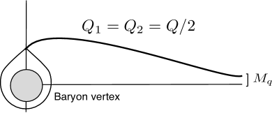
Figure 1: Schematic figure of D-brane configuration for (a) symmetric matter and (b) asymmetric matter.

3.1 $D4$ brane background

Here we consider probe $D6$, $D4$ and $D2$ branes in the $D4$ background which is given by

$$ds_{D4}^{2} = \left(\frac{U}{R}\right)^{3/2}\left(\eta_{\mu\nu}dx^{\mu}dx^{\nu}+f(U)dx_{4}^{2}\right)+\left(\frac{R}{U}\right)^{3/2}\left(\frac{dU^{2}}{f(U)}+U^{2}d\Omega_{4}^{2}\right)$$ (10)

$$e^{\phi} = g_{s}\left(\frac{U}{R}\right)^{3/4},\quad F_{4}=\frac{2\pi N_{c}}{\Omega_{4}}\epsilon_{4},\;\;f(U)=1-\Big{(}\frac{U_{KK}}{U}\Big{)}^{3},\;\;R^{3}=\pi g_{s}N_{c}l_{s}^{3}.$$ (11)

The Kaluza-Klein mass scale $M_{KK}$ is defined as inverse radius of the $x_{4}$ direction: $M_{KK}=\frac{3}{2}\frac{U^{1/2}_{KK}}{R^{3/2}}$. The bulk parameters, $U_{KK},g_{s},R$ and the gauge theory parameters $M_{KK},g^{2}_{YM},\lambda:=g_{YM}^{2}N_{c}$ are related by

$$g_{s}=\frac{\lambda}{2\pi l_{s}N_{c}M_{KK}},\quad U_{KK}=\frac{2}{9}\lambda M_{KK}l_{s}^{2},\quad R^{3}=\frac{\lambda l_{s}^{2}}{2M_{KK}}.$$ (12)

We introduce new coordinate $\bar{\xi}$ by $\frac{d\bar{\xi}^{2}}{\bar{\xi}^{2}}=\frac{dU^{2}}{U^{2}f(U)}$ and obtain, in Euclidean signature,

$$ds_{D4}^{2}=\left(\frac{U}{R}\right)^{3/2}\left(dt^{2}+d\vec{x}^{2}+f(U)dx_{4}^{2}\right)+\left(\frac{R}{U}\right)^{3/2}\left(\frac{U}{\bar{\xi}}\right)^{2}\left(d\bar{\xi}^{2}+\bar{\xi}^{2}d\Omega_{4}^{2}\right)\,.$$ (13)

The relation between $U$ and $\bar{\xi}$ is

$$U^{3/2}=\bar{\xi}^{3/2}\left[1+\left(\frac{\bar{\xi}_{KK}}{\bar{\xi}}\right)^{3}\right]\equiv\bar{\xi}^{3/2}\omega_{+},$$ (14)

where $U_{KK}^{3/2}=2\bar{\xi}_{KK}^{3/2}$. We rescale $\bar{\xi}=\bar{\xi}_{KK}\xi$ such that singularity is located at $\xi=1$. Then the background (13) and the dilaton can be rewritten as

$$ds_{D4}^{2} = \left(\frac{\bar{\xi}_{KK}}{R}\right)^{3/2}\xi^{3/2}\omega_{+}\left(dt^{2}+d\vec{x}^{2}+f(U)dx_{4}^{2}\right)+\left(R^{3}\bar{\xi}_{KK}\right)^{1/2}\frac{\omega_{+}^{1/3}}{{\xi}^{3/2}}\left(d{\xi}^{2}+{\xi}^{2}d\Omega_{4}^{2}\right),$$ (15)

$$e^{\phi} = \left(\frac{\bar{\xi}_{KK}}{R}\right)^{3/4}{\xi}^{3/4}\omega_{+}^{1/2}.$$ (16)

The baryon vertex in this background is a spherical $D4$ brane wrapping $S^{4}$. The induced metric on compact $D4$ brane is given by (see 94 for the detail),

$$ds_{BV}^{2}=\left(\frac{\bar{\xi}_{KK}}{R}\right)^{3/2}{\xi}^{3/2}\omega_{+}dt^{2}+\left(R^{3}\bar{\xi}_{KK}\right)^{1/2}\omega_{+}^{1/3}{\xi}^{1/2}\left[\left(1+\frac{{\xi^{\prime}}^{2}}{\xi^{2}}\right)d\theta^{2}+\sin^{2}\theta d\Omega_{3}^{2}\right].$$ (17)

The free energy of the compact $D4$ can be written as

$${\cal F}_{BV}=\tau_{4}\int d\theta\sqrt{\omega_{+}^{4/3}(\xi^{2}+\xi^{\prime 2})}\sqrt{\tilde{D}(\theta)^{2}+\sin^{6}\theta},$$ (18)

with

$$\tilde{D}(\theta)=-2+3(\cos\theta-\frac{1}{3}\cos^{3}\theta).$$ (19)

The embeddings of baryon $D4$ brane can be obtained as a function of $\xi_{0}$, the position of $D4$ brane at $\xi=0$. From the embedding solution, we can get value of $\xi$ and its slope at $\theta=\pi$ which will be used in force balance condition. The details of the embeddings are discussed in [16].

Now we add probe brane in this geometry; we can put $D6$, $D4$ and $D2$ brane corresponding to the $3+1$, $2+1$ and $1+1$ theory at the boundary. The general induced metric on $Dq(q=6,4,2)$ brane can be written from (82)

$$ds_{D_{q}}^{2} \!= \!\left(\frac{\bar{\xi}_{KK}}{R}\right)^{3/2}\xi^{3/2}\omega_{+}\left(dt^{2}+d\vec{x}_{d}^{2}\right)$$ (21)

$$~{}~{}~{}~{}~{}~{}~{}~{}~{}~{}+\left(R^{3}\bar{\xi}_{KK}\right)^{1/2}\frac{\omega_{+}^{1/3}}{\xi^{3/2}}\left[\left(1+\dot{Y}^{2}\right)d\rho^{2}+\rho^{2}d\Omega_{q-d-1}^{2}\right].$$

From (91), we can write the free energy of $Dq$ brane as follows

$${\cal F}_{Dq}=\hat{\tau}_{q}\int d\rho\sqrt{\omega_{+}^{4/3}(1+\dot{Y}^{2})}\sqrt{\hat{Q}^{2}+\rho^{2n}\omega_{+}^{\frac{4}{3}(d-1)}},$$ (22)

where $n=q-d-1$ and $\hat{\tau}_{q}\equiv\tau_{q}\bar{\xi}_{KK}^{d}$. $\hat{Q}$ is related to the number of source $Q$ as follows

$$\hat{Q}=\frac{Q}{\tau_{q}(2\pi\alpha^{\prime})\bar{\xi}_{KK}^{(d-1)}}.$$ (23)

The boundary condition is described in the appendix B (113). We now can solve the equation of motion with force balance condition for given $\hat{Q}$.

For the nuclear symmetry energy (9) in large $N_{c}$ theory, we need to define what is the proton and neutron. In the case of $N_{c}=3$, proton consists of two up quark and one down quark(uud), and neutron is udd. But in generic $N_{c}$, it is not clear what is the quark contents of proton and neutron. There are many possibilities for quark configurations of proton and neutron but we consider two possibilities in Figure 2.

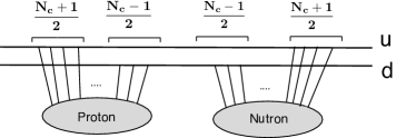
Figure 2: proton and neutron in generic $N_{c}$.

$\bullet$ case (a): In this case, the difference of quark number between proton and neutron is always $1$. To make this configuration be possible, we assume that $N_{c}$ is odd. From this configuration, we can set

$$Q_{1}-Q_{2}=N_{p}-N_{n},~{}~{}~{}~{}~{}Q_{1}+Q_{2}=Q=N_{B}N_{c},$$ (24)

where $N_{p}$ is number of proton and $N_{n}$ is number of neutron. Then, $\tilde{\alpha}$ can be written as

$$\tilde{\alpha}=\frac{Q_{1}-Q_{2}}{Q_{1}+Q_{2}}=\frac{N_{p}-N_{n}}{N_{c}N_{B}},$$ (25)

and

$$Q_{1}=\frac{1+\tilde{\alpha}}{2}N_{c}N_{B},~{}~{}~{}~{}~{}Q_{2}=\frac{1-\tilde{\alpha}}{2}N_{c}N_{B}.$$ (26)

From this definition, the second order term becomes

$$\tilde{\alpha}^{2}E_{2}=\left(\frac{N_{p}-N_{n}}{N_{c}N_{B}}\right)^{2}E_{2}=\left(\frac{N_{p}-N_{n}}{N_{B}}\right)^{2}\cdot\frac{E_{2}}{N_{c}^{2}}.$$ (27)

Then, the symmetry energy per nucleon can be identified as

$$S_{2}=\frac{E_{2}}{N_{c}^{2}N_{B}}.$$ (28)

From (5), we can get symmetry energy per nucleon in terms of elements of induced metric,

$$S_{2}=\frac{\bar{\xi}_{KK}}{\pi\alpha^{\prime}}\cdot\frac{1}{N_{C}}\int d\rho\frac{\hat{Q}\sqrt{\omega_{+}^{4/3}(1+\dot{Y}^{2})}\,\,\rho^{2n}\omega_{+}^{\frac{4}{3}(d-1)}}{\left(\hat{Q}^{2}+4\rho^{2n}\omega_{+}^{\frac{4}{3}(d-1)}\right)^{3/2}}.$$ (29)

There is $1/N_{C}$ factor in the symmetry energy (29) which implies that the symmetry energy is suppressed by $N_{C}$. It is consistent with the definition of proton and neutron: there is only one quark difference between proton and neutron and therefore, for large $N_{C}$, it is not easy to distinguish these two particle and hence symmetry energy becomes zero for large $N_{C}$. $\bullet$ case (b): In this case, proton consist of $N_{C}-1$ up quarks and one down quark, and neutron has single up quark and $N_{C}-1$ down quark. The total difference and total number can be written in term of proton and neutron number as follows

$$Q_{1}-Q_{2}=(N_{C}-2)(N_{p}-N_{n}),~{}~{}~{}~{}~{}Q_{1}+Q_{2}=N_{C}N_{B}.$$ (30)

Then,

$$\tilde{\alpha}=\frac{Q_{1}-Q_{2}}{Q_{1}+Q_{2}}=\frac{(N_{C}-2)(N_{p}-N_{n})}{N_{C}N_{B}},$$ (31)

and

$$\tilde{\alpha}^{2}E_{2}=\left(\frac{N_{p}-N_{n}}{N_{B}}\right)^{2}\cdot\frac{(N_{C}-2)^{2}}{N_{C}^{2}}E_{2}.$$ (32)

Performing same procedure with previous case, we get symmetry energy as follows;

$$S_{2}=\frac{\bar{\xi}_{KK}}{\pi\alpha^{\prime}}\cdot\frac{(N_{C}-2)^{2}}{N_{C}}\int d\rho\frac{\hat{Q}\sqrt{\omega_{+}^{4/3}(1+\dot{Y}^{2})}\,\,\rho^{2n}\omega_{+}^{\frac{4}{3}(d-1)}}{\left(\hat{Q}^{2}+4\rho^{2n}\omega_{+}^{\frac{4}{3}(d-1)}\right)^{3/2}}.$$ (33)

Instead of suppression by $N_{C}$, the symmetry energy grows with $N_{C}$ factor for large $N_{C}$ limit.

Considering other intermediate case in similar fashion, we can easily see that the free energy should be lowest in the case (a). Therefore we take the definition of proton defined in (a). We can convert all parameters in terms of physical quantities such as ’t Hooft coupling $\lambda$, Kaluza-Klein scale $M_{KK}$ and density. The nuclear density and quark mass can be written as

$$\varrho = \frac{Q}{N_{c}V_{d}}=\frac{2^{(d-1)/3}\Omega_{n}}{3^{2(d-1)}(2\pi)^{n+d-1}}\lambda^{d-2}M_{KK}^{d}\hat{Q},$$ (34)

$$m_{q} = \frac{\lambda M_{KK}Y_{\infty}}{2^{2/3}\cdot 9\pi},$$ (36)

and the coefficient in (29) becomes $\frac{\bar{\xi}_{KK}}{\pi\alpha^{\prime}}=\frac{2^{1/3}}{9\pi}\lambda M_{KK}.$ By substituting these numerical solution into (9) we can get symmetry energy for each embeddings in terms of density and quark mass. From the meson mass calculation, we choose

$$\lambda=18,\;\;M_{KK}=1.04GeV,\;\;N_{C}=3.$$ (37)

With this values we can calculate density and quark mass dependence of symmetry energy for $D6$, $D4$ and $D2$ probe brane cases. See Figure 3.

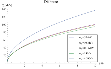
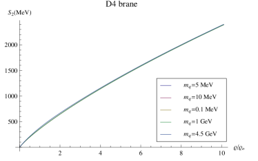
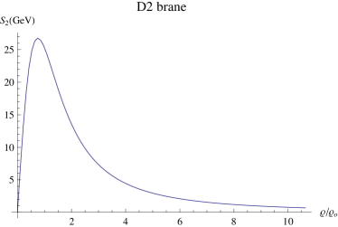
Figure 3: Density dependence of symmetry energy for several quark mass for (a) D6 probe brane, (b) D4 probe brane and (c) D2 probe brane.

$\bullet$ $D6$ probe brane:
In this case, the boundary theory is in $3+1$ dimension. From the Figure 3 (a), the symmetry energy with D6 probe brane seems to have square root behavior. All the lines are well fitted to $S_{2}=S_{0}(\varrho/\varrho_{0})^{1/2}$, with $27{\rm MeV}\leq S_{0}\leq 36{\rm MeV}$. For small quark mass($5{\rm MeV}$), symmetry energy curve is fitted to $S_{2}\sim 28({\rm MeV})(\varrho/\varrho_{0})^{1/2}$. As quark mass increase, the symmetry energy curve move downwards, in other words, it become softer up to quark mass is around 100 MeV. After then, the symmetry energy curve moves to upwards(stiffer) as quark mass increases.

$\bullet$ $D4$ probe brane:
The dual theory lives in 2+1 dimension and the result is drawn in Figure 3 (b). In this figure, most symmetry energy curves are on top of each other unless quark mass is very large. And it’s behavior seems to be linear for small density.

$\bullet$ $D2$ probe brane:
In this case, dual theory is of 1+1 dimensional. The density dependence in the free energy (22) factors out:

$${\cal F}_{D_{2}}=\hat{\tau}_{2}\int d\rho\sqrt{\hat{Q}^{2}+1}\sqrt{\omega_{+}^{4/3}(1+\dot{Y}^{2})},$$ (38)

so that the embedding configuration is independent of density. The symmetry energy can be written as follows

$$S_{2}=\frac{\bar{\xi}_{KK}}{4\pi\alpha^{\prime}}\frac{\hat{Q}}{(\hat{Q}^{2}+4)^{3/2}}\int d\rho\sqrt{\omega_{+}^{4/3}(1+\dot{Y}^{2})}.$$ (39)

The embedding configuration looks flat for any quark mass which means that the symmetry energy is almost same for all quark mass region. See Figure. 3 (c).

3.2 $D3$ brane background

We now consider the confining geometry based on $D3$ brane [21];

$$ds_{10}^{2}=e^{\phi/2}\left(\frac{r^{2}}{R^{2}}A^{2}(r)\eta_{\mu\nu}dx^{\mu}dx^{\nu}+\frac{R^{2}}{r^{2}}dr^{2}+R^{2}d\Omega_{5}^{2}\right),$$ (40)

where $A(r)$ and the dilaton are given by:

$$A(r)=\left(1-\left(\frac{r_{0}}{r}\right)^{8}\right)^{1/4}\qquad\&\qquad e^{\phi}=\left(\frac{(r/r_{0})^{4}+1}{(r/r_{0})^{4}-1}\right)^{\sqrt{3/2}}\,,$$ (41)

while the five-form remains unaltered from the pure $AdS$ solution. $R$ is the $AdS$ radius and $r_{0}$ is the position of the singularity determined by the value of gluon condensation. Unlike D4 brane background, the exact relation between $r_{0}$ and $<G^{2}>$ is not clear. So we will see power behavior of symmetry energy in terms of density and asymptotic value of probe brane. For simplicity, we set $r_{0}=1$. Procedding similarly with the previous section, we can get Hamiltonian for baryon $D5$ brane;

$${\cal F}_{BV}=\tau_{5}\int d\theta A(r)\sqrt{e^{\phi}(r^{\prime 2}+r^{2})}\sqrt{D(\theta)^{2}+\sin^{8}\theta}\,,$$ (42)

where,

$$D(\theta)=-\frac{3}{2}\theta+\frac{3}{2}\sin\theta\cos\theta+\sin^{3}\theta\cos\theta\,.$$ (43)

The details of this embedding are discussed in [22]. We add $D7$, (or $D5$, $D3$) brane as a probe. The induced metric on $Dq$ brane can be written as

$$ds_{Dq}^{2}=e^{\phi/2}\left[\frac{r^{2}}{R^{2}}A^{2}(r)(dt^{2}+d\vec{x}_{d}^{2})+\frac{R^{2}}{r^{2}}\left\{(1+\dot{Y}^{2})d\rho^{2}+\rho^{2}d\Omega_{q-d-1}^{2}\right\}\right].$$ (44)

And the free energy for probe brane is

$${\cal F}_{Dq} = \tau_{q}\int d\rho\sqrt{e^{\phi}A(r)^{2}(1+\dot{Y}^{2})}\sqrt{\tilde{Q}^{2}+e^{\frac{\phi}{2}(q-5)}A(r)^{2d}\rho^{2n}}\,.$$ (45)

The symmetry energy(9) becomes

$$S_{2}=\frac{1}{4\pi\alpha^{\prime}}\int d\rho\frac{\tilde{Q}\rho^{2n}e^{\frac{\phi}{2}(q-4)}A(r)^{2d+1}\sqrt{1+\dot{Y}^{2}}}{\left(\tilde{Q}^{2}+4e^{\frac{\phi}{2}(q-5)}A(r)^{2d}\rho^{2n}\right)^{3/2}}.$$ (46)

With same method of the previous section, we can calculate symmetry energy, see Figure 4.

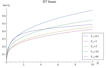
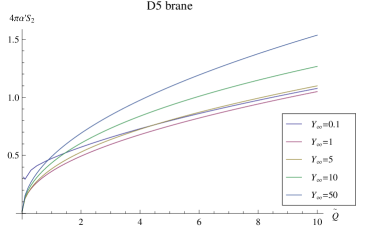
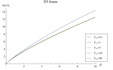
Figure 4: Density dependence of symmetry energy for several quark mass.

$\bullet$ $D7$ probe brane:
In this case, the corresponding boundary boundary theory is of 3+1 dimension. The density and $Y_{\infty}$ dependence of symmetry energy is drawn in Figure4. In this figure, one can see that symmetry energy has power behavior unless asymptotic value of probe brane($Y_{\infty}=0.1$) is very small. Actually, the symmetry energy curves with $1\leq Y_{\infty}\leq 50$ behave as

$$S_{2}\simeq\frac{S_{0}}{4\pi\alpha^{\prime}}\tilde{Q}^{1/3},$$ (47)

with $0.21\leq S_{0}\leq 0.31$.

$\bullet$ $D5$ probe brane:
The boundary theory is of 2+1 dimension and the symmetry energy behaves

$$S_{2}\simeq\frac{S_{0}}{4\pi\alpha^{\prime}}\tilde{Q}^{1/2},$$ (48)

with $0.34\leq S_{0}\leq 0.5$ unless $Y_{\infty}$ is very small, see Figure 4 (b).

$\bullet$ $D3$ probe brane:
The boundary theory is of 1+1 dimension. We can see the symmetry energy grows linearly for small density, see Figure 4 (c).

For the given boundary space-time, the density dependence of symmetry energy seems to depend on the dimensionality of D-brane system we use. For the 3+1 dimensional boundary theory, the probe brane should be $D6$ for $D4$ brane background and it should be $D7$ for $D3$ background. In the case of $D6$ brane, $S_{2}\sim\varrho^{1/2}$. On the other hand $S_{2}\sim\varrho^{1/3}$ for $D7$ probe in $D3$ background. These differences appear in all other probe brane cases as well. We will discuss these phenomena further later.

4 Symmetry energy in quark matter system

So far, we discuss symmetry energy in confined system. In this section we consider symmetry energy in deconfined phase, namely, in quark matter instead of nuclear matter. The background geometry is a black brane. To introduce finite density or chemical potential, we introduce fundamental strings which connect black hole horizon and probe brane. The end points of fundamental strings attached on probe provide sources of $U(1)$ gauge field. Since the fundamental strings can move freely along the $D3$ direction of the black brane horizon, the boundary system can be identified as the system of freely moving quarks.

Similarly to the previous section, the symmetry energy can be understood as the energy cost to separate the number of up and down quarks from symmetric matter. From the D-brane point of view, we need to consider two probe branes, where different number of strings are attached so that the embedding of two branes are separated from each other. The schematic figure is drawn in Figure 5.

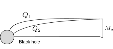
Figure 5: Schematic figure of D-brane configuration for (a) symmetric matter and (b) asymmetric matter.

The boundary condition at the horizon is determined by the regularity of the equation of motion at the horizon;

$$\dot{Y}_{\rho_{min}}=\tan\theta,$$ (49)

where $\theta$ is the angle of probe brane at the horizon. By substituting the embedding solution into (9), we can get symmetry energy as a function of density and quark mass.

4.1 $D4$ brane background

To describe deconfined phase at the boundary theory, we introduce black hole geometry based on D4 brane;

$$ds^{2} = \left(\frac{U}{R}\right)^{3/2}\left(f(U)dt^{2}+d\vec{x}^{2}+dx_{4}^{2}\right)+\left(\frac{R}{U}\right)^{3/2}\left(\frac{dU^{2}}{f(U)}+U^{2}d\Omega_{4}^{2}\right)$$ (50)

$$e^{\phi} = g_{s}\left(\frac{U}{R}\right)^{3/4},\quad F_{4}=\frac{2\pi N_{c}}{\Omega_{4}}\epsilon_{4},\;\;f(U)=1-\Big{(}\frac{U_{0}}{U}\Big{)}^{3},\;\;R^{3}=\pi g_{s}N_{c}l_{s}^{3}.$$ (51)

There is a horizon at $U=U_{0}$, and the Hawking temperature and the horizon radius are related by [23]

$$U_{0}=\frac{16\pi^{2}}{9}R^{3}T^{2}.$$ (52)

Introducing a dimensionless coordinate $\xi$ by $\frac{d\xi^{2}}{\xi^{2}}=\frac{dU^{2}}{U^{2}f(U)}$, the background geometry becomes

$$ds^{2}=\left(\frac{U}{R}\right)^{3/2}\left(f(U)dt^{2}+d\vec{x}^{2}+dx_{4}^{2}\right)+\left(\frac{R}{U}\right)^{3/2}\left(\frac{U}{\xi}\right)^{2}\left(d\xi^{2}+\xi^{2}d\Omega_{4}^{2}\right),$$ (53)

where $U$ and $\xi$ are related by

$$\left(\frac{U}{U_{0}}\right)^{3/2}=\frac{1}{2}\left(\xi^{3/2}+\frac{1}{\xi^{3/2}}\right),\;\;{\rm and}\;\;f=\left(\frac{1-\xi^{-3}}{1+\xi^{-3}}\right)^{2}\equiv\frac{\omega_{-}^{2}}{\omega_{+}^{2}}.$$ (54)

In this geometry, we rescale the coordinates such that the black hole horizon is located at $\xi=1$. The induced metric of probe $Dq$ brane can be written as

$$ds_{Dq}^{2} \!= \!\left(\frac{1}{R}\right)^{3/2}\xi^{3/2}\omega_{+}\left(\frac{\omega_{-}^{2}}{\omega_{+}^{2}}dt^{2}+d\vec{x}_{d}^{2}\right)$$ (56)

$$~{}~{}~{}~{}~{}~{}~{}~{}~{}~{}+R^{3/2}\frac{\omega_{+}^{1/3}}{\xi^{3/2}}\left[\left(1+\dot{Y}^{2}\right)d\rho^{2}+\rho^{2}d\Omega_{q-d-1}^{2}\right].$$

The form of free energy of $D_{q}$ brane can be obtained from (91) as follows

$${\cal F}_{Dq}=\tau_{q}\int d\rho\sqrt{\frac{\omega_{-}^{2}}{\omega_{+}^{2/3}}(1+\dot{Y}^{2})}\sqrt{\tilde{Q}^{2}+\left(\xi^{3/4}\omega_{+}\right)^{d-1}\left(\frac{\rho^{2}\omega_{+}^{1/3}}{\xi^{3/4}}\right)^{n}},$$ (57)

where $n=q-d-1$. By substituting the embedding solution into eq.(9), we can calculate symmetry energy in terms of density $Y_{\infty}$, the asymptotic value of probe brane, which is related to quark mass and temperature by

$$Y_{\infty}=\frac{2\pi l_{s}^{2}}{U_{0}}m_{q}=\frac{9l_{s}}{8\pi R^{3}}\cdot\frac{m_{q}}{T^{2}}.$$ (58)

Therefore, if we fix quark mass, large value of $Y_{\infty}$ corresponds to low temperature and small $Y_{\infty}$ to high temperature.

$\bullet$ $D6$ probe brane:
In this case, at low temperature(large value of $Y_{\infty}$), the symmetry energy $S_{2}=0.5\tilde{Q}^{1/2}$, which is same as confining case. At high temperature(small value of $Y_{\infty}$), symmetry energy increase linearly in density. We can understand this from eq.(9). The symmetry energy is integration of a function from $\rho_{min}$ to infinity. In the case of nuclear matter system, $\rho_{min}$ is zero since the probe brane ends at the tip of baryon vertex. On the other hand, in deconfining phase, probe brane ends on black hole horizon with non-zero $\rho_{min}$. Therefore, embedding for small asymptotic value start near equator $\rho_{min}=1$. If density is small($\tilde{Q}<<1$), we can ignore $\tilde{Q}^{2}$ term in denominator and symmetry energy is just linear in $\tilde{Q}$. However, for low temperature, $Y_{\infty}$ is small and $\rho_{min}\to 0$ and therefore $\tilde{Q}^{2}$ in the denominator contributes to the integral by scaling the variables, giving the power behavior we observed above. The result is described in the figure 6(a).

$\bullet$ $D4$ probe brane:
In the case of $D4$ probe brane, we get similar result in confining case which is lineally increase as density increase. See the figure 6(b).

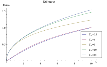
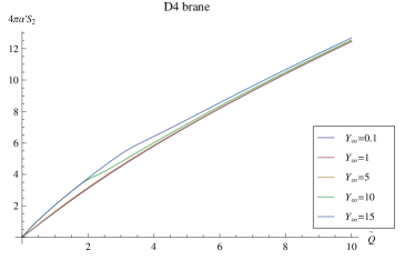
Figure 6: Density dependence of symmetry energy for several $Y_{\infty}$.

$\bullet$ $D2$ probe brane:
For $D2$ brane case symmetry energy become

$$S_{2}\sim\frac{\hat{Q}}{(\hat{Q}^{2}+4)^{3/2}}\int d\rho\sqrt{\frac{\omega_{-}^{2}}{\omega_{+}^{2/3}}(1+\dot{Y}^{2})},$$ (59)

which is also independent of details of embedding. And the result is almost same as Figure 3(c).

4.2 $D3$ brane background

We now consider the black $D3$ brane geometry;

$$ds^{2} = \frac{U^{2}}{R^{2}}\left(f(U)dt^{2}+d\vec{x}^{2}\right)+R^{2}\left(\frac{dU^{2}}{f(U)U^{2}}+d\Omega_{5}^{2}\right),$$ (60)

where $R^{4}=2\lambda l_{s}^{4}$ and $f(U)=1-\left({U_{0}}/{U}\right)^{4}$. Here, $\lambda=g_{YM}^{2}N_{c}$ is the ’t Hooft coupling of the YM theory. There is a horizon at $U=U_{0}$, and the Hawking temperature is given by

$$T=\frac{U_{0}}{\pi R^{2}}=\frac{U_{0}}{\sqrt{2\lambda}\pi l_{s}^{2}}.$$ (61)

Introducing a dimensionless coordinate $\xi$ defined by ${d\xi^{2}}/{\xi^{2}}={dU^{2}}/({U^{2}f(U)})$, the bulk geometry becomes

$$ds^{2} = \frac{U^{2}}{R^{2}}\left(fdt^{2}+d\vec{x}^{2}\right)+\frac{R^{2}}{\xi^{2}}\left(d\xi^{2}+\xi^{2}d\Omega_{5}^{2}\right),$$ (62)

where $\xi^{2}\equiv y^{2}+\rho^{2}$ and $\rho$ is the radius of the 3-sphere. $U$ and $\xi$ are related by ${U^{2}}/{U_{0}^{2}}=\frac{1}{2}(\xi^{2}+{1}/{\xi^{2}})\,$ and $f=({1-\xi^{4}})^{2}/({1+\xi^{4}})^{2}.$ The induced metric on $Dq$ probe brane and Hamiltonian density can be written as follows

$$ds_{Dq}^{2} = \frac{\xi^{2}\omega_{+}}{R^{2}}\left(\frac{\omega_{-}^{2}}{\omega_{+}^{2}}dt^{2}+d\vec{x}_{d}^{2}\right)+\frac{R^{2}}{\xi^{2}}\left[(1+\dot{Y}^{2})d\rho^{2}+\rho^{2}d\Omega_{q-d-1}^{2}\right]$$ (63)

$${\cal H}_{Dq} = \tau_{q}\sqrt{\frac{\omega_{-}^{2}}{\omega_{+}}(1+\dot{Y}^{2})}\sqrt{\tilde{Q}^{2}+\rho^{2n}\omega_{+}^{d}}.$$ (65)

With completely same method with the previous section, we calculate symmetry energy for each probe brane($D7$, $D5$ and $D3$) in terms of density and asymptotic value of probe brane $Y_{\infty}$. In this case, the relationship beetween the asymptotic value of probe brane and temperature(or quark mass) is given by

$$Y_{\infty}=\frac{2m_{q}}{\sqrt{\lambda}T}.$$ (66)

The result is drawn in Figure 7.

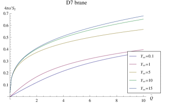
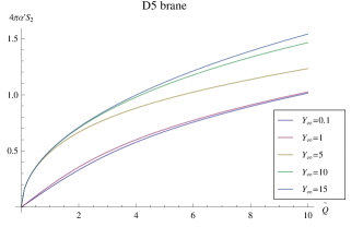
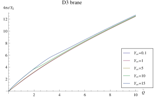
Figure 7: Density dependence of symmetry energy for several $Y_{\infty}$.

Same as the previous section, we fix quark mass. Then, the asymptotic value of probe brane $Y_{\infty}$ proportional to the inverse temperature. In the case of $D7$ brane, for low temperature($Y_{\infty}=15$), the symmetry energy goes like $S_{2}=0.32\tilde{Q}^{1/3}$ while at high temperature, the symmetry energy grows linearly. The symmetry energy line at low temperature for $D5$ probe case goes like $S_{2}=0.5\tilde{Q}^{1/2}$ and it becomes linear at high temperature. In the case of $D3$ probe, symmetry energy has linear behavior for all temperature.

5 Scaling property and universality classes

In this section, we want to understand the scaling behavior of the symmetry energy which is calculated in various models and various phases. We first tabulate all the results in table 1 and table 2.

Table 1: $D4$ brane background

	0	1	2	3	4	5	6	7	8	9	$q$	$d$	$q-d-1$	$S_{2}$	$2\nu=n/d$
$D4$	$\bullet$	$\bullet$	$\bullet$	$\bullet$	$\bullet$
$D2$	$\bullet$	$\bullet$				$\bullet$					2	1	0	${\cal O}(1)$	-
$D4$	$\bullet$	$\bullet$	$\bullet$			$\bullet$	$\bullet$				4	2	1	$Q$	$1/2$
$D6$	$\bullet$	$\bullet$	$\bullet$	$\bullet$		$\bullet$	$\bullet$	$\bullet$			6	3	2	$Q^{1/2}$	$2/3$

Table 2: $D3$ brane background

	0	1	2	3	4	5	6	7	8	9	$q$	$d$	$q-d-1$	$S_{2}$	$2\nu=n/d$
$D3$	$\bullet$	$\bullet$	$\bullet$	$\bullet$
$D3$	$\bullet$	$\bullet$			$\bullet$	$\bullet$					3	1	1	$Q$	1
$D5$	$\bullet$	$\bullet$	$\bullet$		$\bullet$	$\bullet$	$\bullet$				5	2	2	$Q^{1/2}$	1
$D7$	$\bullet$	$\bullet$	$\bullet$	$\bullet$	$\bullet$	$\bullet$	$\bullet$	$\bullet$			7	3	3	$Q^{1/3}$	1

We emphasize that the result is based on the actual numerical calculation without any approximation.

We now re-derive these power behavior of symmetry energy analytically. To do this, we consider the ideally simplified case: BPS metric background and flat embedding of probe branes. In this case, background geometry becomes geometry of black $Dq$ brane;

$$ds_{10}^{2}=Z_{p}^{-1/2}(-dt^{2}+d\vec{x}_{p}^{2})+Z_{p}^{1/2}d\vec{x}_{\perp}^{2},$$ (67)

with $e^{2\phi}=Z_{p}^{\frac{3-p}{2}}.$ We now consider the general result for the symmetry energy

$$S_{2}=2\tau_{q}\int d\rho\frac{\tilde{Q}\sqrt{G_{tt}G_{\rho\rho}}e^{-2\phi}G_{xx}^{d}G_{\Omega\Omega}^{n}}{\left(\tilde{Q}^{2}+4e^{-2\phi}G_{xx}^{d}G_{\Omega\Omega}^{n}\right)^{3/2}}.$$ (68)

which is already given in eq. (9). Then, the term in the square root becomes 1 and

$$e^{-2\phi}G_{xx}^{d}\left(\frac{G_{\perp\perp}}{\xi^{2}}\right)^{q-d-1} = Z_{p}^{\frac{p-3}{2}}\cdot Z_{p}^{-\frac{d}{2}}\cdot Z_{p}^{\frac{q-d-1}{2}}$$ (69)

$$= Z_{p}^{\frac{1}{2}(p+q-2d-4)}.$$ (70)

The value of $p+q-2d$ is precisely equal to the number of Neuman-Dirichlet (ND) direction of $Dp/Dq$ system. Therefore, if we focus on the system which is supersymmetric configurations or a smooth deformation of them, the exponent becomes zero. In this case the symmetry energy (9) for flat embedding can be calculated analytically:

$$S_{2} = 2\tau_{q}\int d\rho\frac{\tilde{Q}\rho^{2n}}{\left(\tilde{Q}^{2}+4\rho^{2n}\right)^{3/2}}=c_{n}\tilde{Q}^{\frac{1}{n}},$$ (71)

where $c_{n}=2\tau_{q}\frac{2^{-2-1/n}\Gamma\left(\frac{1}{2n}\right)\Gamma\left(\frac{n-1}{2n}\right)}{n^{2}\sqrt{\pi}}$ and $n=q-d-1$ so that the density dependence of symmetry energy is $S_{2}\sim Q^{\frac{1}{q-d-1}}$. This result reproduces all the result we obtained in previous section numerically.

Notice that both the background and embedding used here are far from the real situation: real background is a deformation of such BPS solution and the embedding is non-trivial deformation from such a flat embedding. Nevertheless, the scaling exponent is the same as the actual configuration used for numerical computation of previous sections. The point is that neither smooth deformation of the metric nor the deformation of the embedding shape seem to change the scaling behavior of the symmetry energy. The exponent of symmetry energy depends only on the dimensionality of probe brane and dimension of non-compact directions. Therefore the scaling exponents depend only on the universality classes.

6 Discussion

In this paper, we calculated the asymmetry energy for both nuclear matter as well as the quark matter. The symmetry energy has a power like density dependence with characteristic exponent which is invariant under the smooth deformation of the metric as well as smooth deformation of the embedding. It only depends on the dimensionality of the D-brane system modeling the QCD dynamics. Therefore it is a index for the universality class. The physical interpretation of the scaling exponent is still open question but we give a trial interpretation below.

Discussion: Non-fermi liquid nature of the nuclear matter. According to the fermi gas model of nuclei, the Energy of the nuclei is the sum of the kinetic energies of neutrons and protons which are moving non-relativistically, namely,

$$E = \frac{3}{5}(N_{p}\epsilon_{Fp}+N_{n}\epsilon_{Fn})$$ (72)

$$= \frac{3}{5}\epsilon_{F}A+\frac{1}{3}\epsilon_{F}A\delta^{2}+{\cal O}(\delta^{4}),$$ (73)

where $A=N_{p}+N_{n}$ is the mass number and $\epsilon_{F}$ is the fermi energy for $A$, $\delta=\frac{(N_{p}-N_{n})}{(N_{p}+N_{n})}$. One can see that the symmetry energy per nucleon is $\epsilon_{F}/3$. Therefore fermi gas model demonstrates the origin of the symmetry energy as the Pauli principle. What happens if we include the interaction energy of the nucleons? The answer is largely unknown. Depending on how one includes the interaction, the answers are different from one another. In some of the traditional approach, interactions are taken care of by adding a polynomial in density, which means that scaling property ($\sim\rho^{\alpha}$) should be destroyed by the interaction. However, this is not what we get. In our approach, scaling property remains even in the large density limit. Notice that for the most interesting case of $D4$/$D6$ and $D3$/$D7$, the scaling exponents are $1/2$ and $1/3$ respectively. Comparing this with the non-interacting gas which gives $S_{2}\sim\rho^{2/3}$, one can see that the symmetry energy of $D4$/$D6$ implies an anomalous dispersion relations which is neither relativistic nor non-relativistic one. For the $D3$/$D7$ case, the scaling is the same as the relativistic particles. If we naively extrapolate the relation $S_{2}\sim\epsilon_{F}$, $S_{2}\sim\rho^{1/2}$ means the anomalous dispersion relation $\epsilon\sim k^{3/2}$. One may want to associate this as the example of transformation of a particle to un-particle [24]

One may also expect that such anomalous dispersion relation is related to the non-fermi liquid nature of the strongly interacting fermion system. In the presence of the fermi sea, one expect that elementary excitations are quasi particles with renormalized charge and mass. However, when the interactions are strong, such quasi-particles will lose applicability. Using the AdS/CFT duality and utilizing the AdS at UV and the $AdS_{2}$ at the IR, it was shown in[25] that

$$G(\omega,k)=\frac{1}{\omega-v_{F}k_{\perp}-C\omega^{2\nu}},$$ (74)

where $k_{\perp}$ is the momentum measured from the fermi surface. If $\nu<1/2$, the dispersion relation becomes $\omega\sim k_{\perp}^{1/2\nu}$. For example, if $\nu=1/3$ we get $\omega\sim k_{\perp}^{3/2}$. In our case, the situation is more subtle since the fermi surface is not stable under turning on temperature and fermi sea is not so calm: the low lying states below ‘fermi sea’ can be all excited so that it should be called fermi ball [26] rather than fermi surface, and $k_{\perp}$ should be replace by $k$. These phenomena are all beyond the fermi liquid behavior. For D3/D7 case, the exponent indicate that the system is marginally fermi liquid case. More systematic investigation on this matter is strongly desired.

Appendix A Free energy of $Dq$ brane

We start from 10 dimensional metric for $Dp$ brane with Lorenzian signature as

$$ds_{10}^{2} = -G_{tt}dt^{2}+G_{xx}d\vec{x}_{p}^{2}+G_{rr}dr^{2}+G_{\perp\perp}d\Omega_{\perp}^{2}$$ (75)

$$= -G_{tt}dt^{2}+G_{xx}d\vec{x}_{p}^{2}+G_{\perp\perp}\left(\frac{G_{rr}}{G_{\perp\perp}}dr^{2}+d\Omega_{\perp}^{2}\right),$$ (76)

where $d\Omega_{\perp}^{2}$ is metric of $S^{(8-p)}$. To make the orthogonal space to $Dp$ brane, we introduce new coordinate;

$$\sqrt{\frac{G_{rr}}{G_{\perp\perp}}}dr=\frac{d\xi}{\xi},$$ (77)

then, the metric (75) becomes

$$ds_{10}^{2}=-G_{tt}dt^{2}+G_{xx}d\vec{x}_{p}^{2}+\frac{G_{\perp\perp}}{\xi^{2}}\left(d\xi^{2}+\xi^{2}d\Omega_{\perp}^{2}\right).$$ (78)

Now, we put probe $Dq$ brane in this background with $d$ dimensional uncompact direction. We can decompose transverse direction into parallel and perpendicular to the probe brane as follows

$$ds_{10}^{2} = -G_{tt}dt^{2}+G_{xx}(d\vec{x}_{d}^{2}+d\vec{x}_{p-d}^{2})+\frac{G_{\perp\perp}}{\xi^{2}}\left(dR_{q-d}^{2}+dR_{9-p-q+d}^{2}\right)$$ (79)

$$= -G_{tt}dt^{2}+G_{xx}(d\vec{x}_{d}^{2}+d\vec{x}_{p-d}^{2})$$ (81)

$$+\frac{G_{\perp\perp}}{\xi^{2}}\left(d\rho^{2}+\rho^{2}d\Omega_{q-d-1}^{2}+dY^{2}+Y^{2}d\Omega_{8-p-q+d}\right).$$

We assume that only $Y$ coordinate has $\rho$ dependence and the other coordinates which perpendicular to probe brane is constant, then the induce metric on probe brane can be written as

$$ds_{Dq}^{2} = -G_{tt}dt^{2}+G_{xx}d\vec{x}_{d}^{2}+\frac{G_{\perp\perp}}{\xi^{2}}(1+\dot{Y}^{2})d\rho^{2}+\frac{G_{\perp\perp}}{\xi^{2}}\rho^{2}d\Omega_{q-d-1}^{2}$$ (82)

$$\equiv -G_{tt}dt^{2}+G_{xx}d\vec{x}_{d}^{2}+G_{\rho\rho}d\rho^{2}+G_{\Omega\Omega}d\Omega_{q-d-1}^{2},$$ (83)

where $\dot{Y}=\partial Y/\partial\rho$.

To introduce number density in boundary theory, we turn on time component of $U(1)$ gauge field $A_{t}(\rho)$ on the probe brane and set all the other components to be zero. Then we can write DBI action as follows;

$$S_{Dq} = -\mu_{q}\int d\sigma^{q+1}e^{-\phi}\sqrt{{\rm det}(g+2\pi\alpha^{\prime}F)}$$ (84)

$$= -\mu_{q}\int dt\,d^{d}x\,d\Omega_{q-d-1}\,d\rho\,e^{-\phi}\sqrt{G_{xx}^{d}G_{\Omega\Omega}^{q-d-1}(G_{tt}G_{\rho\rho}-\tilde{F}^{2})}$$ (85)

$$\equiv \int dt\,d\rho\,{\cal L}_{Dq},$$ (86)

where $\tilde{F}\equiv=2\pi\alpha^{\prime}F_{t\rho}=2\pi\alpha^{\prime}\partial_{\rho}A_{t}(\rho)$.

From the equation of motion for gauge field, we can define conserved charge;

$$\frac{\partial{\cal L}_{Dq}}{\partial\tilde{F}}=\frac{\tau_{q}e^{-\phi}G_{xx}^{d}G_{\Omega\Omega}^{q-d-1}\tilde{F}}{\sqrt{G_{xx}^{d}G_{\Omega\Omega}^{q-d-1}(G_{tt}G_{\rho\rho}-\tilde{F}^{2})}}\equiv\frac{Q}{2\pi\alpha^{\prime}},$$ (87)

where $\tau_{q}=\mu_{q}V_{d}\Omega_{q-d-1}$. Then we can get the relation between field strength and charge as

$$\tilde{F}=\frac{\tilde{Q}\sqrt{G_{tt}G_{\rho\rho}}}{\sqrt{\tilde{Q}^{2}+e^{-2\phi}G_{xx}^{d}G_{\Omega\Omega}^{q-d-q}}},$$ (88)

where $\tilde{Q}=Q/2\pi\alpha^{\prime}\tau_{q}$.

After Legengdre transformation for Lagrangian density, we can get free energy of $D_{q}$ brane;

$${\cal F}_{Dq} = \int d\rho\left(\tilde{F}\frac{\partial{\cal L}_{Dq}}{\partial\tilde{F}}-{\cal L}_{Dq}\right)$$ (89)

$$= \tau_{q}\int d\rho\sqrt{G_{tt}G_{\rho\rho}}\sqrt{\tilde{Q}^{2}+e^{-2\phi}G_{xx}^{d}G_{\Omega\Omega}^{q-d-1}}$$ (90)

$$= \tau_{q}\int d\rho\sqrt{G_{tt}\frac{G_{\perp\perp}}{\xi^{2}}(1+\dot{Y}^{2})}\sqrt{\tilde{Q}^{2}+e^{-2\phi}\,G_{xx}^{d}\left(\frac{G_{\perp\perp}}{\xi^{2}}\rho^{2}\right)^{q-d-1}}.$$ (91)

Appendix B Baryon vertex and force balance condition

In this work, we consider $D3$ or $D4$ brane as a background. In $D3$ brane background, $D5$ brane wrapping on $S^{5}$ with $N_{c}$ fundamental strings is interpreted as baryon vertex and a spherical $D4$ brane on $S^{4}$ is baryon vertex in $D4$ brane background. In the both case, background metric can be written in general form;

$$ds_{10}^{2} = -G_{tt}dt^{2}+G_{xx}d\vec{x}_{p}^{2}+\frac{G_{\perp\perp}}{\xi^{2}}\left(d\xi^{2}+\xi^{2}d\Omega_{8-p}^{2}\right)$$ (92)

$$= -G_{tt}dt^{2}+G_{xx}d\vec{x}_{p}^{2}+\frac{G_{\perp\perp}}{\xi^{2}}d\xi^{2}+G_{\perp\perp}\left(d\theta^{2}+\sin^{2}\theta d\Omega_{7-p}^{2}\right),$$ (93)

here, we assume that the $D(8-p)$ brane has $SO(7-p)$ symmetry, then $\xi$ depends on polar angle $\theta$ only. Then the induced metric on $D(8-p)$ brane is

$$ds_{BV}^{2}=-G_{tt}dt^{2}+\frac{G_{\perp\perp}}{\xi^{2}}\left(\xi^{2}+\xi^{\prime 2}\right)d\theta^{2}+G_{\perp\perp}\sin^{2}\theta d\Omega_{7-p}^{2}.$$ (94)

The DBI action for $D(8-p)$ brane can be written as followes;

$$S_{BV}=-\mu_{8-p}\int d^{9-p}\sigma e^{-\phi}\sqrt{{\rm det}(g+2\pi\alpha^{\prime}F)}+\mu_{8-p}\int 2\pi\alpha^{\prime}A_{t}\wedge G_{(7-p)},$$ (95)

where $\mu_{8-p}$ is a D-brane tension and $G_{(7-p)}$ is Ramon-Ramon field which couples to the original $Dp$ brane. After substituting induce metric (94), we can get

$$S_{BV} = \tau_{8-p}\int dtd\theta\sin^{(7-p)}\theta\left[-R^{(p-7)}e^{-\phi}G_{\perp\perp}^{\frac{7-p}{2}}\sqrt{\frac{G_{tt}G_{\perp\perp}}{\xi^{2}}\left(\xi^{2}+\xi^{\prime 2}\right)-\tilde{F}^{2}}+(7-p)\tilde{A}_{t}\right]$$ (96)

$$\equiv \int dtd\theta{\cal L}_{BV},$$ (97)

where

$$\tau_{8-p}=\mu_{8-p}\Omega_{7-p}R^{7-p},~{}~{}~{}~{}\tilde{A}_{t}=2\pi\alpha^{\prime}A_{t}.$$ (98)

The displacement can be obtained by derivative the action with respect to $\tilde{F}$,

$$\frac{\partial{\cal L}_{BV}}{\partial\tilde{F}}=\frac{\tau_{8-p}R^{p-7}\sin^{7-p}\theta e^{-\phi}G_{\perp\perp}^{\frac{7-p}{2}}\cdot\tilde{F}}{\sqrt{\frac{G_{tt}G_{\perp\perp}}{\xi^{2}}\left(\xi^{2}+\xi^{\prime 2}\right)-\tilde{F}^{2}}}\equiv-D(\theta),$$ (99)

and the equation of motion for gauge field is given by

$$\partial_{\theta}\tilde{D}(\theta)=-(7-p)\sin^{7-p}\theta,$$ (100)

where $\tilde{D}(\theta)\equiv D(\theta)/\tau_{8-p}$. By integrating, we get the solution in terms of hypergeometric function as follows

$$\tilde{D}(\theta)=c_{0}+(7-p)\cos\theta\,\,_{2}F_{1}\left(\frac{1}{2},\frac{p-6}{2},\frac{3}{2},\cos^{2}\theta\right).$$ (101)

For example, in the case of $D4$ brane $(p=4)$, we get

$$\tilde{D}(\theta)=c_{0}+\cos\theta(3-\cos^{2}\theta),$$ (102)

which is same as result in [16]. The integration constant $c_{0}$ is determined such that $\tilde{D}$ vanishes at $\theta=0$ which means all fundamental strings are attached on north pole of $D(8-p)$ brane. After substituting the solution of equation of motion, we can rewrite DBI action in terms of displacement which is called as ’Hamilotnian’ because the procedure to get it is similar to Legendre transformation.

$${\cal H}_{BV}=\tau_{8-p}\sqrt{\frac{G_{tt}G_{\perp\perp}}{\xi^{2}}\left(\xi^{2}+\xi^{\prime 2}\right)}\sqrt{\tilde{D}^{2}+R^{2(p-7)}\sin^{2(7-p)}\theta\,\,e^{-2\phi}G_{\perp\perp}^{7-p}}.$$ (103)

As discussed in previous works, we can calculate force at the cusp of single $D(8-p)$ brane as follows,

$$F_{BV} = \frac{\delta{\cal H}_{BV}}{\delta\xi_{c}}\Bigg{|}_{\rm on-shell}=\frac{\partial{\cal H}_{BV}}{\partial\xi^{\prime}}\Bigg{|}_{\theta=\pi}$$ (104)

$$= \tau_{8-p}\frac{(7-p)\sqrt{\pi}\Gamma\left(\frac{8-p}{2}\right)}{2\cdot\Gamma\left(\frac{9-p}{2}\right)}\sqrt{\frac{G_{tt}G_{\perp\perp}}{\xi_{c}^{2}}}\frac{\xi_{c}^{\prime}}{\sqrt{\xi_{c}^{2}+\xi_{c}^{\prime 2}}}$$ (106)

$$= \frac{N_{c}}{2\pi\alpha^{\prime}}\sqrt{\frac{G_{tt}G_{\perp\perp}}{\xi_{c}^{2}}}\cdot\frac{\xi_{c}^{\prime}}{\sqrt{\xi_{c}^{2}+\xi_{c}^{\prime 2}}},$$ (108)

where $\xi_{c}$ and $\xi_{c}^{\prime}$ denote to the value of $\xi$ and it’s derivative at the cusp. The overall factor becomes $N_{c}/2\pi\alpha^{\prime}$ for both of $D3$ and $D4$ case.

Now, we can get boundary condition for probe $Dq$ brane by imposing ’force balance condition’. The force at the cusp of probe brane can be obtained from Hamiltonian of probe brane (91);

$$F_{Dq} = \frac{\delta{\cal H}_{Dq}}{\delta Y_{c}}\Bigg{|}_{\rm on-shell}=\frac{\partial{\cal H}_{Dq}}{\partial\dot{Y}}\Bigg{|}_{\rho=0}$$ (109)

$$= \frac{Q}{2\pi\alpha^{\prime}}\sqrt{\frac{G_{tt}G_{\perp\perp}}{\xi_{c}^{2}}}\frac{\dot{Y_{c}}}{\sqrt{1+\dot{Y_{c}}^{2}}},$$ (111)

where $Y_{c}$ and $\dot{Y}_{c}$ denote to the value of $Y$ and it’s derivative at the cusp of probe brane. From the force balance condition

$$F_{Dq}(Q)=N_{B}\cdot F_{BV}=\frac{Q}{N_{c}}F_{BV},$$ (112)

we can get the boundary condition for probe brane

$$\dot{Y}_{c}=\frac{\xi_{c}^{\prime}}{Y_{c}}$$ (113)

which does not depends on type of original brane or probe brane.

References

- [1] P. Danielewicz, R. Lacey, and W. G. Lynch, Science 298, 1592 (2002).
- [2] A.W. Steiner, M. Prakash, J. Lattimer, and P. J. Ellis, Phys. Rept. 411, 325 (2005).
- [3] B.-A Li, L.-W. Chen and C. M. Ko, Phys. Rept. 464, 113 (2008).
- [4] C. Xu and B. A. Li, Phys. Rev. C 81, 064612 (2010) [arXiv:0910.4803 [nucl-th]].
- [5] D.V. Shetty and S.J. Yennello, Pramana 75 259 (2010).
- [6] M. Di Toro, V. Baran, M. Colonna, and V. Greco, J. Phys. G 37, 083101 (2010).
- [7] H. K. Lee, B. Y. Park and M. Rho, Phys. Rev. C 83, 025206 (2011) [arXiv:1005.0255 [nucl-th]].
- [8] Z. Xiao, B.-A. Li, L.-W. Chen, G.-C. Yong, and M. Zhang, Phys. Rev. Lett. 102, 062502 (2009).
- [9] L.W. Chen, C.M. Ko, and B.A. Li, Phys. Rev. Lett. 94, 032701 (2005).
- [10] Y. Kim, Y. Seo, I. J. Shin and S. -J. Sin, JHEP 1106, 011 (2011) [arXiv:1011.0868 [hep-ph]].
- [11] J. M. Maldacena, J.M. Maldacena, Adv. Theor. Math. Phys. 2, 231 (1998), Int. J. Theor. Phys. 38, 1113 (1999).
- [12] S. S. Gubser, I. R. Klebanov and A. M. Polyakov, Phys. Lett. B428, 105 (1998).
- [13] E. Witten, Adv. Theor. Math. Phys. 2, 253 (1998).
- [14] M. Kruczenski, D. Mateos, R. C. Myers and D. J. Winters, JHEP 0405, 041 (2004) [arXiv:hep-th/0311270].
- [15] T. Sakai and S. Sugimoto, Prog. Theor. Phys. 113, 843 (2005) J. Erlich, E. Katz, D. T. Son and M. A. Stephanov, Phys. Rev. Lett. 95, 261602 (2005) L. Da Rold and A. Pomarol, Nucl. Phys. B 721, 79 (2005)
- [16] Y. Seo and S.-J. Sin, JHEP 0804, 010 (2008).
- [17] Y. Kim, Y. Seo, and S.-J. Sin, JHEP 1003, 074 (2010).
- [18] E. Witten, JHEP 9807, 006 (1998). [hep-th/9805112].
- [19] S. S. Gubser, hep-th/9902155.
- [20] N. J. Evans, S. D. H. Hsu and M. Schwetz, Phys. Lett. B 382, 138 (1996) [arXiv:hep-ph/9605267].
-
[21]
S. S. Gubser,
arXiv:hep-th/9902155.
A. Kehagias and K. Sfetsos, Phys. Lett. B 454 (1999) 270 - [22] Y. Seo, J. P. Shock, S. -J. Sin, D. Zoakos, JHEP 1003, 115 (2010). [arXiv:0912.4013 [hep-th]].
- [23] M. Kruczenski, D. Mateos, R. C. Myers and D. J. Winters, JHEP 0405, 041 (2004) [arXiv:hep-th/0311270].
- [24] H. Georgi, Int. J. Mod. Phys. A 25, 573 (2010).
- [25] T. Faulkner, H. Liu, J. McGreevy and D. Vegh, Phys. Rev. D 83, 125002 (2011) [arXiv:0907.2694 [hep-th]].
- [26] S. -S. Lee, Phys. Rev. D 79, 086006 (2009) [arXiv:0809.3402 [hep-th]].