Extremal polygons in $\mathbb{R}^{3}$

Abstract.

The oriented area function $A$ is (generically) a Morse function on the space of planar configurations of a polygonal linkage. We are lucky to have an easy description of its critical points as cyclic polygons and a simple formula for the Morse index of a critical point. However, for planar polygons, the function $A$ in many cases is not a perfect Morse function. In particular, for an equilateral pentagonal linkage it has one extra local maximum (except for the global maximum) and one extra local minimum.

In the present paper we consider the space of 3D configurations of a polygonal linkage. For an appropriate generalization $S$ of the area function $A$ the situation becomes nicer: we again have an easy description of critical points and a simple formula for the Morse index. In particular, unlike the planar case, for an equilateral linkage with odd number of edges the function $S$ is always a perfect Morse function and fits the lacunary principle. Therefore cyclic equilateral polygons can be interpreted as independent generators of the homology groups of the (decorated) configuration space.

1. Introduction

The oriented area function $A$ is (generically) a Morse function on the space of planar configurations of a polygonal linkage. We are lucky to have an easy description of its critical points as cyclic polygons (Theorem 2.4), and a simple formula for the Morse index of a critical point (Theorem 2.5). However, for planar polygons, in many cases $A$ is not a perfect Morse function. In particular, for an equilateral pentagonal linkage it has one extra local maximum (except for the global maximum) and one extra local minimum, see Example 2.6. For an equilateral heptagonal linkage the number of Morse points greatly exceeds the sum of Betti numbers of the configuration space, and it is unclear how the boundary homomorphisms of the Morse chain complex look like.

Surprisingly, if we pass to $\mathbb{R}^{3}$, for an appropriate generalization $S$ of the area function $A$ the situation becomes nicer. We again have an easy description of critical points (as SW-invariant configurations, see Theorem 5.3), and a simple formula for the Morse index (Theorems 5.5). In particular, unlike the planar case, for an equilateral linkage with odd number of edges $S$, all critical points have even Morse indices. By the lacunary principle, $S$ is a perfect Morse function (see Theorem 6.8) and the Morse chain complex has zero boundary homomorphisms. As a direct corollary we interpret cyclic equilateral polygons as independent generators of the homology groups of the configuration space.

Acknowledgements. I’m indebted to George Khimshiashvili, Dirk Siersma, Alena Zhukova, and Mikhail Khristoforov for inspiring conversations.

2. Preliminaries and notation

A polygonal $n$-linkage is a sequence of positive numbers $L=(l_{1},\dots,l_{n})$. It should be interpreted as a collection of rigid bars of lengths $l_{i}$ joined consecutively by revolving joints in a chain.

Definition 2.1.

A configuration of $L$ in the Euclidean space $\mathbb{R}^{d}$, $d=2,\ 3$ is a sequence of points $R=(p_{1},\dots,p_{n+1}),\ p_{i}\in\mathbb{R}^{d}$ with $l_{i}=|p_{i},p_{i+1}|$ and $l_{n}=|p_{n},p_{1}|$ modulo the action of orientation preserving isometries of the space $\mathbb{R}^{d}$. We also call $P$ a closed chain or a polygon.

The set $M_{d}(L)$ of all configurations is the moduli space, or the configuration space of the polygonal linkage $L$.

A configuration carries a natural orientation which we indicate in figures by an arrow.

We explain below in this paragraph what is known about planar configurations and the signed area function as the Morse function on the configuration space.

Definition 2.2.

The signed area of a polygon $P$ with the vertices
$p_{i}=(x_{i},y_{i})$ is defined by

$$2A(P)=(x_{1}y_{2}-x_{2}y_{1})+\ldots+(x_{n}y_{1}-x_{1}y_{n}).$$

Definition 2.3.

A polygon $P$ is called cyclic if all its vertices $p_{i}$ lie on a circle.

Cyclic polygons arise here as critical points of the signed area:

Theorem 2.4.

[6] Generically, a polygon $P$ is a critical point of the signed area function $A$ iff $P$ is a cyclic configuration. ∎

Theorem 2.5.

[7],[11] For a generic cyclic configuration $P$ of a linkage $L$,

$$\mu(P)=\left\{\begin{array}[]{ll}e(P)-1-2\omega_{P}&\hbox{if }\ \delta(P)>0;\\ e(P)-2-2\omega_{P}&\hbox{otherwise}.\end{array}\right.$$

Here we used the below notation:

Notation for cyclic configurations, see Fig. 1.

$r$ is the radius of the circumscribed circle.

$\alpha_{i}$ is the half of the angle between the vectors $\overrightarrow{Op_{i}}$ and $\overrightarrow{Op}_{i+1}$. The angle is defined to be positive, orientation is not involved.

$\omega_{P}$ is the winding number of $P$ with respect to the center $O$.

$\mu(P)$ is the Morse index of the function $A$ in the point P. That is, $\mu(P)$ is the number of negative eigenvalues of the Hessian $Hess_{P}(A)$.

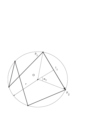
Figure 1. Basic notation for a pentagonal cyclic configuration with $E=(-1,-1,-1,1,-1)$

A cyclic configuration is called central if one of its edges contains $O$.

For a non-central configuration, let $\varepsilon_{i}$ be the orientation of the edge $p_{i}p_{i+1}$, that is,

$\varepsilon_{i}=\left\{\begin{array}[]{ll}1,&\hbox{if the center $O$ lies to the left of }p_{i}p_{i+1};\\ -1,&\hbox{if the center $O$ lies to the right of }p_{i}p_{i+1}.\end{array}\right.$

$E(P)=(\varepsilon_{1},\dots,\varepsilon_{n})$ is the string of orientations of all the edges.

$e(P)$ is the number of positive entries in $E(P)$.

Example 2.6.

[9] An equilateral pentagonal linkage $L=(1,1,1,1,1)$ has 14 cyclic configurations indicated in Fig. 4.

(1). The convex regular pentagon and its mirror image are the global maximum and minimum of the signed area $A$. Their Morse indices are $2$ and $0$ respectively.

(2). The starlike configurations are a local maximum and a local minimum of $A$.

(3). There are $10$ more configurations that have three consecutive edges aligned. Their Morse indices equal $1$.

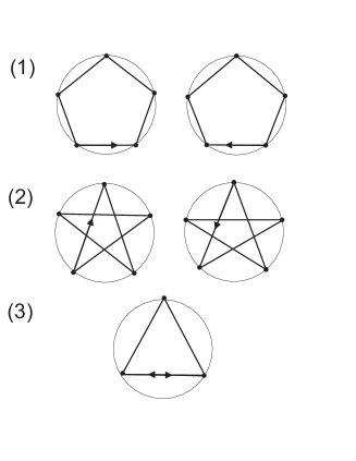
Figure 2. Cyclic configurations of the equilateral pentagonal linkage

3. The decorated moduli space $\widetilde{\mathcal{M}}_{3}(L)$ and the function $S$

We have already defined the moduli space $M_{3}(L)$. However, it is convenient to consider the decorated moduli space:

Definition 3.1.

The decorated moduli space is defined as the set of pairs

$$\widetilde{M}_{3}(L)=\{(P,\xi)|P\ \hbox{is a polygon in $\mathbb{R}^{3}$ with the sidelengths}\ l_{1},...,l_{n};\ \xi\in S^{2},\}$$

factorized by the diagonal action of the orientation preserving isometries of $\mathbb{R}^{3}$.

Here $S^{2}\in\mathbb{R}^{3}$ is the unit sphere centered at the origin $O$.

Lemma 3.2.

The space $\widetilde{M}_{3}(L)$ is an orientable fibration over $M_{3}(L)$ whose fiber is $S^{2}$.

Proof. The set of all polygons with fixed sidelengths (before factorization by isometries) is known to be orientable. Therefore the set of the pairs (a polygon, a vector) is also orientable as a trivial fibration. Since we take a factor by the action of orientation preserving isometries, the result is also orientable.∎

Lemma 3.3.

The Euler class of the fibration equals zero.

Proof. Indeed, $\xi(P)=\frac{\overrightarrow{p_{1}p_{2}}}{|p_{1}p_{2}|}$ defines an everywhere non-zero section. ∎

Corollary 3.4.

(The Gisin sequence for the decorated moduli space) We have the following short exact sequence:

$$0\rightarrow H^{m}(M(L))\rightarrow H^{m}(\widetilde{M}(L))\rightarrow H^{m-2}(M(L))\rightarrow 0.$$

Proof. This follows directly from Gisin sequence, see [10]. ∎

Definition 3.5.

Let $(P,\xi)\in\widetilde{M}_{3}(L)$, let $(x_{i},y_{i})$ be the vertices of $P$. The vector area of the pair $(P,\xi)$ is defined as the following scalar product:

$$2S(P,\xi)=(p_{1}\times p_{2}+p_{2}\times p_{3}+\dots+p_{n}\times p_{1},\xi).$$

An alternative equivalent definition is:

$$S(P,\xi)=A(pr_{\xi^{\perp}}(P)),$$

where $pr_{\xi^{\perp}}$ is the plane orthogonal to $\xi$ and cooriented by $\xi$.

4. Swap action

We assume that a polygonal linkage $L$ with all $l_{i}$ different is fixed. We make a convention that the numbering is modulo $n$, that is, for instance, $n+1=1$.

Definition 4.1.

1. Let $P\in M_{2}(L)$ be a polygon. For $i=1,\dots,n$, denote by $s_{i}(P)$ the polygon obtained from $P$ by transposing of the two edges adjacent to the vertex $p_{i}$ (see Fig. 3).

2. For $P\in M_{3}(L)$, the polygon $s_{i}(P)$ is obtained from $P$ by the above rules. We assume that the new pair of edges lies in the plane spanned by the two old edges.

3. For $(P,\xi)\in\widetilde{M}_{3}(L)$ we define $s_{i}(P,\xi)=(s_{i}(P),\xi).$

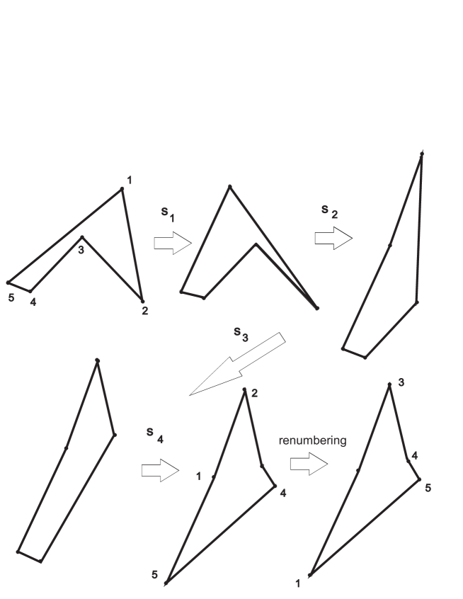
Figure 3. The mapping $SW$

We get homeomorphisms $s_{i}:M_{2,3}(L)\rightarrow M_{2,3}(\sigma_{i}L),$ and $s_{i}:\widetilde{M}_{3}(L)\rightarrow\widetilde{M}_{3}(\sigma_{i}L),$ where $\sigma_{i}$ is the element of the symmetric group $\sigma_{i}\in S_{n}$ is a transposition induced by $s_{i}$.

Denote also by $SW(P)$ the polygon $s_{n-1}\circ...\circ s_{2}\circ s_{1}(P)$ whose vertices are renumbered in such a way (that is, with a shift by one) that $SW$ becomes a (smooth) automorphism of $M_{2,3}(L)$.

Lemma 4.2.

The actions of $s_{i}$ and of $SW$ respect the functions $A$ and $S$. ∎

Theorem 4.3.

A polygon $P\in M_{2}(L)$ is $SW$-invariant (that is, $SW(P)$ equals $P$ up to an orientation preserving isometry) iff $P$ is cyclic. ∎

5. Critical points and the Morse index

Theorem 5.1.

Generically, critical points $(P,\xi)$ of the function $S$ fall into three classes:

• Planar cyclic configurations. These are pairs $(P,\xi)$ such that $P$ is a planar cyclic polygon, and $\xi$ is orthogonal to the affine hull of $P$.

• Non-planar configurations. They are characterized by the three following conditions:

  1. The vectors $\xi$ and $\overrightarrow{S}=p_{1}\times p_{2}+p_{2}\times p_{3}+\dots+p_{n}\times p_{1}$ are parallel (but they can have opposite directions).

  2. The orthogonal projection of $P$ onto the plane $\overrightarrow{S(P)}^{\perp}$ is a cyclic polygon.

  3. For every $i$, the vectors $\overrightarrow{T_{i}}$, $\overrightarrow{S}$, and $\overrightarrow{d_{i}}$ are coplanar.

  Here $\overrightarrow{d_{i}}$ is the $i$-th short diagonal, $\overrightarrow{T_{i}}$ is the vector area of the triangle $p_{i-1}p_{i}p_{i+1}$, see Fig. 4.

• Zig-zag planar configurations (existing only for even $n$). The polygon lies in a plane. There are two parallel lines $l_{1}$ and $l_{2}$ such that all the vertices with even indices lie on the line $l_{1}$, whereas all the vertices with odd indices lie on the line $l_{2}$. The vector $\xi$ is parallel to $l_{1,2}$.

For all three cases, if $(P,\xi)$ is a critical point, then $(P,-\xi)$ is critical as well.

Proof. This follows from [8], where we proved nearly the same theorem. ∎

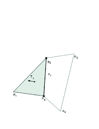
Figure 4. Notation for a non-planar critical polygon

Figure 5. A zigzag critical polygon

Lemma 5.2.

An equilateral polygon with odd number of edges has no non-planar critical configurations.

A shorter characterization of critical points is given in the following analogue of Theorem 4.3:

Theorem 5.3.

Generically, $(P,\xi)$ is a critical point of the vector area function $S$ if and only if $P$ is SW-invariant. ∎

An crucial fact about non-planar configurations is the following: Let $(P,\xi)$ be a non-planar critical configuration. As Theorem 5.1 says, the orthogonal projection $prP$ on $\xi^{\perp}$ is cyclic.

Lemma 5.4.

For a non-planar critical configuration,

$$\delta(prP)=0.$$

Proof. We use notations $r,pr_{i},h_{i}$ for the radius of the circle, lengths of the projections, and heights differences. We have the following closing condition $\sum_{i=1}^{n}h_{i}=0$. Note that the angle $\alpha_{i}(prP)$ equals the angle between the chord $pr_{i}$ and the circumscribed circle. The conditions from Theorem 5.1 imply that the fraction $\frac{h_{i}}{pr_{i}}cos\ \alpha_{i}$ does not depend on $i$. Denote the latter by $h$. The closing condition implies

$$0=\sum_{i=1}^{n}h_{i}=\frac{2h}{r}\sum_{i=1}^{n}\frac{pr_{i}/2r}{cos\ \alpha_{i}}=\frac{2h}{r}\sum_{i=1}^{n}tan\ \alpha_{i}.\qed$$

Theorem 5.5.

Let $(P,\xi)$ be a planar cyclic critical point of $S$.

For the Morse index of the function $S$, we have:

$$\mu(P,\xi)=2e(P)-2\omega_{P}-2.\qed$$

The theorem will be proven in the next section.

On the one hand, we can say nothing about the Morse index of a non-planar critical polygon. On the other hand, in many cases this result is sufficient for a construction of a complete Morse theory on the configuration space. For instance, this is the case for an equilateral polygon with odd number of edges, see Theorem 6.8.

Corollary 5.6.

If all SW-invariant configurations of a polygonal linkage are planar, then

1. The function $S$ is a perfect Morse function.

2. The odd-dimensional homology groups of $M_{3}(L)$ vanish.

3. The even-dimensional homology groups are free abelian, whose rank can be expressed in terms of the number of cyclic configurations of $L$.

∎

6. Proofs for the Section 5. The equilateral polygon

The Betti numbers and the Euler characteristic of the space $M_{3}(L)$ are already known due to A. Klyachko. Namely, he proved the following:

Theorem 6.1.

[5] The following formulae for the Betti numbers are valid:

$$\beta^{2p}(M_{3}(L))-\beta^{2(p-1)}(M_{3}(L)) = \left(\!\!\!\begin{array}[]{c}n-1\\ p\end{array}\!\!\!\right)-\sharp\{I\;|\;l_{I}>l/2;|I|=p+1\}=$$

$$= \sharp\{I\;|\;l_{I}<l/2;\;|I|=p+1\}-\left(\!\!\!\begin{array}[]{c}n-1\\ p+1\end{array}\!\!\!\right),$$

Here $l=l_{1}+l_{2}+\cdots+l_{n}$, $\ l_{I}=\sum_{i\in I}l_{i}$.

In the case of equal lengths the formulae may be simplified.

Proposition 6.2.

[5] For odd $n=2k+1\geq 3$ the Betti numbers of $M_{3}(1,...,1)$ are given by the formula

$$\beta^{2p}(M_{3}(1,...,1))=\sum_{0\leq i\leq p}\left(\!\!\begin{array}[]{c}2k\\ i\end{array}\!\!\right),\;\;p<k;$$

Corollary 6.3.

For Betti numbers of the decorated moduli space $\widetilde{\beta}^{2p}_{n}=\beta^{2p}(\widetilde{M}_{3}(1,...,1))$ we have

$$\widetilde{\beta}^{2p}_{n}=\sum_{0\leq i\leq p}\left(\!\!\begin{array}[]{c}n\\ i\end{array}\!\!\right),\;\;p<k;$$

These expressions can be interpreted them as the numbers of cyclic equilateral polygons:

Lemma 6.4.

Let $n=2k+1$ be an even number.

1. For $p=0,1,...,k$ denote by $N^{p}_{n}$ the number of such cyclic equilateral polygons for which

   $$2e-2\omega-2=2p.$$

   Then

   $$\widetilde{\beta}^{2p}_{n}=N^{p}_{n}.$$

2. $S$ is a perfect Morse function on the configuration space $\widetilde{M}_{3}(1,1,...,1)$.

Proof. (1) Indeed, it is easy to find all cyclic equilateral polygons: first we choose $i$ negatively oriented edges and then choose the winding number that ranges from $\pm 1$ to $\pm(k-i)$.

As an illustration, figures 6 and 9 list all cyclic equilateral pentagons and heptagons.

(2) By Lemma 5.4, equilateral (or, for the sake of generity, nearly equilateral) polygonal linkages with odd number of edges have only planar critical configurations. (1) implies that the number of all critical points equals the sum of all Betti numbers.∎

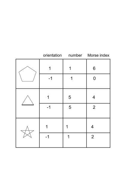
Figure 6. Critical equilateral pentagons and their Morse indices

Cyclic deformations

The key idea of how to find the Morse index of a critical point is to deform the linkage in such a way that the Morse index does not change.

We start with a planar cyclic configuration $(P,\xi)$. A cyclic deformations of a linkage is a one-parametric continuous family arising through the following construction. Let $(P,\xi)$ be a planar cyclic configuration of $L$. We fix the radius $r$ of the circumscribed circle and the vector $\xi$, and force the vertices $p_{i}$ to move along the circle. This yields a continuous family of linkages $L(t)$ together with a continuous family of their cyclic configurations $P(t)$.

We have to understand how the Morse index $\mu(P,\xi)$ changes during the deformation.

There are only two types of events when $\mu(P,\xi)$ can change:

1. If two consecutive vertices $p_{i}$ and $p_{i+1}$ meet, and the edge $l_{i}$ vanishes. This will be called contraction of the edge $l_{i}$. At such a point the dimension of the configuration space decreases.

2. If the point $(P,\xi)$ meets another critical point. If this happens, the value of $\delta(P)$ becomes zero.

Lemma 6.5.

If a cyclic deformation $P(t)$ does not pass through a zero of the function $\delta$ and has no edge contraction, the Morse index $m(P(t))$ remains constant.∎

On the one hand, a detailed analysis of how the Morse index changes when passing through a zero of $\delta$ provides a proof of Theorem 5.5. This proof is independent on the Klyachko’s result 6.2.

On the other hand, there exists a shorter proof (the one presented below), which relies however on the Klyachko’s Theorem 6.2.

Lemma 6.6.

1. Contraction of a negatively oriented edge does not change the Morse index.

2. Contraction of a positively oriented edge turns $\mu$ to $\mu-2$.∎

Lemma 6.7.

Let $P=P(0)$ be a planar cyclic polygon. There exists its cyclic deformation $P(t)$ such that

1. $\delta(P(t))$ is never zero.

2. $P(1)$ is an equilateral star with odd number $n=2k+1$ of edges and with $\omega=k$.

   For such a deformation, we have

   $$\mu(P(1),\xi)=\mu(P,\xi)-2\sharp(\hbox{number of of positively oriented edges contracted.})$$

Figures 7 and 8 present examples of such deformations.∎

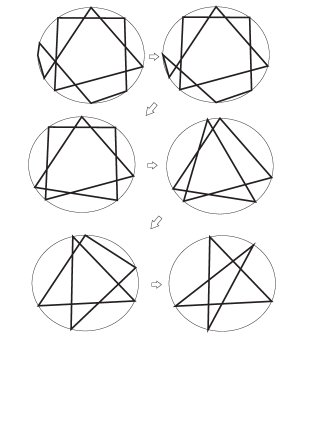
Figure 7. A deformation taking a polygon to an equilateral star

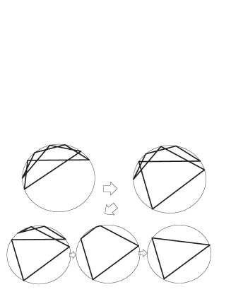
Figure 8. One more deformation taking a polygon to a triangle

Theorem 6.8.

1. Let $L=(1,...,1)$ be an equilateral polygons with odd number of edges. We have the following:

2. The function $S$ is a perfect Morse function on the decorated moduli space $\widetilde{M}_{3}(L)$.

3. The formula for the Morse index from Theorem 5.5 is valid for all critical configurations of $L$.

4. All the Morse indices are even, and the boundary homomorphisms for the Morse chain complex are zero.

5. The equilateral cyclic polygons can be interpreted as independent generators of the homology groups of $\widetilde{M}_{3}(L)$.

Proof. (1) Indeed, by Lemma 5.2 all critical configurations are planar. The number of all cyclic equilateral polygons equals the sum of Betti numbers of the space $\widetilde{M}_{3}(L)$.

(2) We prove this inductively by the number of edges. For $n=5$, this is true by simple reasons. For induction step, assume that the statement is proven for $n=2k+1$. Prove it for $n=2k+3$. Lemma 6.7 determines the Morse indices for the majority of the polygons. For instance, the heptagon number 3 (Fig. 9) after contraction of one negative and one positive edges gives a pentagonal star whose Morse index is already known. There are just two polygons that are irreducible in this sense: the two stars with $\omega=\pm(k+1)$. Since the Morse index of the positively oriented star is bigger than the Morse index of the negatively oriented star, the Morse indices are determined uniquely. The statements (3) and (4) directly follow from (2). ∎

Now we are ready to prove Theorem 5.5. Given a critical point $(P,\xi)$, apply a deformation from Lemma 6.7. It is easy to check that the difference $\mu(P(t),\xi)-2e(P(t),\xi)-2\omega(P(t),\xi)-2$ does not change during the deformation. Besides, by Lemma 6.8, the difference is zero for the endpoint of the deformation. Therefore it is zero at the starting point, that is, for $(P(t),\xi))$.

7. More examples

An equilateral 7-gon

Let $L=(1,1,1,1,1,1,1)$ be an equilateral heptagonal linkage. By Lemma 6.8, $S$ is a perfect Morse function. Figure 9 lists all the types of its critical configurations and their Morse indices.

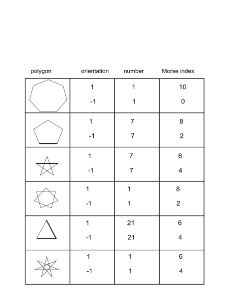
Figure 9. Critical equilateral heptagons and their Morse indices

A nearly equilateral 6-gon

Let $L=(1,1,1,1,1,1-\varepsilon)$. Again, $S$ is a perfect Morse function. Figure 10 lists all the types of its critical configurations and their Morse indices.

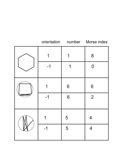
Figure 10. Critical nearly equilateral 6-gons and their Morse indices

A 4-gonal linkage

Let $L=(l_{1},l_{2},l_{3},l_{4})$  be a generic 4-gonal linkage. It is known (see [5]) that $M_{3}(L)=S^{2}$. Corollary 3.4 implies that $H_{0}(\widetilde{M}_{3}(L))=H_{4}(\widetilde{M}_{3}(L))=Z,\ H_{1}(\widetilde{M}_{3}(L))=H_{3}(\widetilde{M}_{3}(L))=0,\ H_{2}(\widetilde{M}_{3}(L))=Z^{2}$. Let us establish this result making use of the Morse complex on the space $\widetilde{M}_{3}(L)$. There are two possible cases:

1. $L$ has only one cyclic configuration which is convex. It gives two Morse points with two opposite vectors $\xi$. One of them is the global maximum of $S$, and the other one – the global minimum. So we have the Morse indices $0$ and $4$. Besides, there are exactly two zig-zag critical points with one and the same polygon $P$ and with two opposite vectors $\xi$. By symmetry reasons, their Morse indices equal 2.

2. $L$ has two cyclic configuration, one is convex and the other one is self-intersecting. Each of them gives two Morse points with two opposite vectors $\xi$. The convex polygon yields the global maximum and the the global minimum. As in the previous case, we have the Morse indices $0$ and $4$. The self-intersecting configuration yields two critical points with Morse indices equal 2.

In both cases the Morse chain complex has zero chain groups with odd indices. Therefore, The odd homology groups are zero, and the even homology groups are free abelian whose rank equals the number of critical points.

A 5-gonal linkage with just two planar configurations

Consider a polygonal linkage

$$L=(1,1,1,1,4-\varepsilon)$$

where $\varepsilon$ is small. There are four critical points: two planar ones (the global maximum and the global minimum of $S$) and two non-planar ones that differ on a mirror symmetry with respect to a plane. Again, $S$ is a perfect Morse function.

References

- [1] Arnold V., Varchenko A., Gusein-Zade S., Singularities of differentiable mappings (Russian). Nauka, Moscow, 2005.
- [2] Cerf J., La stratification naturelle des espaces de fonctions differentiables reelles et le theoreme de la pseudo-isotopie. Inst. Hautes Etudes Sci. Publ. Math., 1970, 39, 169, 5-173.
- [3] Farber M., Schütz D., Homology of planar polygon spaces. Geom. Dedicata, 2007, 125, 18, 75-92.
- [4] Kamiyama, Y., Topology of equilateral polygon linkages. Topology Appl., 1996, 68, 1, 13-31.
- [5] Klyachko A., Spatial polygons and stable configurations of points in the projective line. Tikhomirov, Alexander (ed.) et al., Algebraic geometry and its applications. Proceedings of the 8th algebraic geometry conference, Yaroslavl’, Russia, August 10-14, 1992. Braunschweig: Vieweg. Aspects Math. E 25, 67-84 (1994).
- [6] Khimshiashvili G., Panina G., Cyclic polygons are critical points of area. Zap. Nauchn. Sem. S.-Peterburg. Otdel. Mat. Inst. Steklov. (POMI), 2008, 360, 8, 238–245.
- [7] Khimshiashvili G., Panina G., Siersma D., Zhukova A., Extremal configurations of polygonal linkages. Oberwolfach preprint OWP 2011 - 24, http://www.mfo.de/scientific-programme/publications/owp/2011/
- [8] Khristoforov M., Panina G., Swap action on moduli spaces of polygonal linkages. http://arxiv.org/abs/1107.0126
- [9] Panina G., Zhukova A., Morse index of a cyclic polygon,Cent. Eur. J. Math., 9(2) (2011), 364-377.
- [10] Switzer, R., Algebraic topology–homotopy and homology. Springer-Verlag, 1975.
- [11] Zhukova A., On the Morse index of a cyclic polygon, to appear in St. Petersburg Mathematical Journal.