On Block-Göttsche multiplicities for planar tropical curves.

Abstract.

We prove invariance for the number of planar tropical curves enhanced with polynomial multiplicities recently proposed by Florian Block and Lothar Göttsche. This invariance has a number of implications in tropical enumerative geometry.

1. Introduction

1.1. Some motivations

One of the most classical problem in enumerative geometry is computing the number of curves of given degree $d>0$ and genus $g\geq 0$ that pass through the appropriate number (equal to $3d-1+g$) of generic points in the projective plane ${\mathbb{P}}^{2}$. This problem admits more than one way for interpretation. The easiest and the most well-studied interpretation is provided by the framework of complex geometry. If we take a generic configuration of $3d-1+g$ points in ${\mathbb{C}}{\mathbb{P}}^{2}$ the number of curves will only depend on $d$ and $g$ and not on the choice of points as long as this choice is generic. E.g. for $d=3$ and $g=0$ we always have $12$ such curves. For any given $g$ and $d$ the number can be computed e.g. with the help of the recursive relations of Caporaso-Harris [4].

In this paper we are interested in setting up rather than solving plane enumerative problems. In the world of complex geometry such set up is tautological: all relevant complex curves are treated equally and each contributes 1 to the number we are looking for. (Note that in this case all these complex curves are immersed and have only simple nodes as their self-intersection points.)

A somewhat less well-studied problem appears in the framework of real geometry. For the same $d$ and $g$ but different choices of generic configurations of $3d-1+g$ points the corresponding numbers of real curves can be different. E.g. for $d=3$ and $g=0$ we may have $8$, $10$ or $12$ curves depending on the choice of points (see [5]). It was suggested by Jean-Yves Welschinger [19] to treat real curves differently for enumeration, so that some real curves are counted with multiplicity $+1$ and some with multiplicity $-1$. He has shown that the result is invariant on the choice of generic points if $g=0$. E.g. for the $d=3$, $g=0$ case we always have 8 real curves counted with the Welschinger multiplicity. This number may appear as 8 positive curves, 1 negative and 9 positive curves, or 2 negative and 10 positive curves.

Tropical enumerative geometry encorporates features of both, real and complex geometry. If we fix $3d-1+g$ generic points in the tropical projective plane then the corresponding number of tropical curves of degree $d$ and genus $g$ can be different. Nevertheless, tropical curves may also be prescribed multiplicities in such a way that the resulting number is invariant.

So far two such recipes were known (see [15]): one recovering the number of curves for the complex problem and one recovering the number of curves for the real problem enhanced with multiplicities corresponding to the Welschinger numbers. Note that the real problem is only well-defined (and thus invariant) for the case of $g=0$, but the corresponding tropical real problem is well-defined for arbitrary $g$, see [10].

Recently, a new type of multiplicity for tropical curves were proposed by Florian Block and Lothar Göttsche, [1]. These multiplicities are symmetric Laurent polynomials in one variable with positive integer coefficients. According to the authors of this paper, which should appear soon, their motivation came from a Caporaso-Harris type calculation of the refined Severi degrees (introduced by Göttsche in connection with [12]) that interpolate between the numbers of complex and real curves, see [8]. Accordingly, their multiplicity for tropical curves interpolate between the complex and real multiplicities for tropical curves: the value of the polynomial at 1 is the complex multiplicity while the value at $-1$ is the real multiplicity.

In this paper we show that the Block-Göttsche multiplicity is invariant of the choice of generic tropical configuration of points and thus provides a new way for enumeration of curves in the tropical plane, not unlike quantizing the usual enumeration of curves by integer numbers. E.g. if $d=3$ and $g=0$ then the corresponding number is $y+10+y^{-1}$ that can come from eight curves with multiplicity 1 and one curve of multiplicity $y+2+y^{-1}$, but also may come from nine curves with multiplicity 1 and one curve of multiplicity $y+1+y^{-1}$. The polynomial number of $y+10+y^{-1}$ curves can be thought of as 12 curves from complex enumeration, but now this number decomposes according to different states: 10 “curves” are in the ground state, one “curve” is excited in a $y$-state, while one “curve” is excited in a $y^{-1}$-state. Here we use quotation marks for curves as several of such virtual “curves” correspond to the same tropical curve (e.g. we have one tropical curve of multiplicity $y+1+y^{-1}$, but it correspond to three virtual “curves” in different states).

Our considerations are not limited by curves in the projective planes and include enumeration in all toric surfaces. As the configuration of tropical points is assumed to be generic, we may restrict our attention to $\mathbb{R}^{2}$ (a tropical counterpart of $(\mathbb{C}^{\times})^{2}$) which is dense in any tropical toric surface. The corresponding toric degree is then given by a collection of integer vectors whose sum is zero.

1.2. Tropical curves immersed in the plane

A closed irreducible tropical curve $\bar{C}$ (cf. [16], [18] et al.) is a connected finite graph without 2-valent vertices whose edges are enhanced with lengths. The length of any edge which is not adjacent to a $1$-valent vertex is a positive real number. Any edge adjacent to a $1$-valent vertex is required to have infinite length. Denote the set of 1-valent vertices of $\bar{C}$ with $\partial\bar{C}$. The lengths of the edges induce a complete inner metric on the complement

(1.1) $$C=\bar{C}\smallsetminus\partial\bar{C}.$$

A metric space $C$ is called an open minimal tropical curve if it can be presented by $\eqref{opencurve}$ for some closed irreducible tropical curve $\bar{C}$.

The number $\dim H_{1}(C;\mathbb{R})$ of independent cycles in $C$ is called the genus of the curve $C$.

Definition 1.1 (cf. [15]).

An immersed planar tropical curve is a smooth map $h:C\to\mathbb{R}^{2}$ (in the sense that it is continuous map whose restriction to any open edge is a smooth map between differentiable manifolds), subject to the following properties.

• The map $h$ is a topological immersion.

• For every unit vector $u\in T_{y}(C)$, where $y$ is inside an edge $E\subset C$, we have $(dh)_{y}(u)\in\mathbb{Z}^{2}$. By smoothness, the image $(dh)_{y}(u)$ must be constant on the whole edge $E$ as long as we enhance $E$ with an orientation to specify the direction of the unit vector. We denote $(dh)_{y}(u)$ with $u_{h}(E)$. The GCD of the (integer) coordinates of $u_{h}(E)$ is called the weight $w_{h}(E)$ of the edge $E$.

• For every vertex $v\in C$ we have $\sum\limits_{E}u_{h}(E)=0$, where the sum is taken over all edges adjacent to $v$ and oriented away from $v$. This condition is known as the balancing condition.

Recall that a continuous map is called proper if the inverse image of any compact is compact. A proper immersed tropical curve $h:C\to\mathbb{R}^{2}$ is called simple (see [15]) if it is $3$-valent, the self-intersection points of $h$ are disjoint from vertices, and the inverse image under $h$ of any self-intersection point consists of two points of $C$.

Remark 1.2.

Definition of tropical morphism which is not required to be an immersion, or to spaces other than $\mathbb{R}^{2}$, requires additional conditions which we do not treat here as we do not need them.

By Corollary 2.24 of [15] any simple tropical curve $h:C\to\mathbb{R}^{2}$ locally varies in a $(\varkappa+g-1)$-dimensional affine space $\operatorname{Def}(h)$, where $g$ is the genus of $C$ and $\varkappa$ is the number of infinite edges of $C$. This space has natural coordinates once we choose a vertex $v\in C$. The two of those coordinates are given by $h(v)\in\mathbb{R}^{2}$. The lengths of all closed edges of $C$ give $\varkappa+3g-3$ coordinates (since $h$ is simple the curve $C$ is 3-valent). Then we have $2g$ linear relations (defined over $\mathbb{Z}$) among these lengths as each cycle of $h(C)$ must close up in $\mathbb{R}^{2}$. By Proposition 2.23 of [15] these relations are independent.

Thus the space $\operatorname{Def}(h)$ is an open set in a $(\varkappa+g-1)$-dimensional affine subspace $U\subset\mathbb{R}^{2+\varkappa+3g-3}$. The slope of this affine subspace is integer in the sense that there exist $(\varkappa+g-1)$ linearly independent vectors in $\mathbb{Z}^{2+\varkappa+3g-3}$ parallel to $U$. This enhances the tangent space $T_{h}(U)$ to $\operatorname{Def}(h)$ at $h$ with integer lattice and hence a volume element (defined up to sign).

1.3. Lattice polygons and points in general position

Let $\Delta$ be a finite collection of non-zero vectors with integer coordinates in $\mathbb{R}^{2}$ such that the vectors of $\Delta$ generate $\mathbb{R}^{2}$ and the sum of these vectors is equal to $0$. We call such a collection balanced. The balanced collection $\Delta$ defines a lattice polygon (that is, a convex polygon with integer vertices and non-empty interior) $\Delta^{*}\subset(\mathbb{R}^{2})^{*}$ in the dual vector space $(\mathbb{R}^{2})^{*}$ to $\mathbb{R}^{2}$: each side $s$ of $\Delta^{*}$ is orthogonal to a certain vector $v\in\Delta$ so that $v$ is an outward normal to $\Delta^{*}$ (we say that such a vector $v$ is dual to $s$); the integer length $\#(s\cap\ \mathbb{Z}^{2})-1$ of the side $s$ is equal to the GCD of the two coordinates of the sum of all the vectors in $\Delta$ which are dual to $s$. The collection $\Delta$ defines a lattice polygon $\Delta^{*}$ uniquely up to translation. Denote by $\varkappa(\Delta)$ the number of vectors in $\Delta$, and denote by $\varkappa(\Delta^{*})$ the perimeter $\#(\partial\Delta^{*}\cap\ \mathbb{Z}^{2})$ of $\Delta^{*}$. Clearly, we have $\varkappa(\Delta)\leq\varkappa(\Delta^{*})$.

In general, if a lattice polygon $\Delta^{*}$ is fixed, the collection $\Delta$ cannot be restored uniquely. However, if we assume that all the vectors of $\Delta$ are primitives (that is, the GCD of the coordinates of each vector is $1$ or, alternatively $\varkappa(\Delta)=\varkappa(\Delta^{*})$), then $\Delta^{*}$ defines $\Delta$ in a unique way. A balanced collection $\Delta\subset\mathbb{R}^{2}$ is called primitive if all the vectors of $\Delta$ are primitive.

We say that an immersed planar tropical curve $h:C\to\mathbb{R}^{2}$ is of degree $\Delta$ if the multiset $\{u_{h}(E)\}$, where $E$ runs over the unbounded edges $E\subset C$ oriented towards infinity, coincides with $\Delta$. Denote with ${\mathcal{M}}_{g,\Delta}^{\operatorname{simple}}$ the space of all simple tropical curves of degree $\Delta$ and genus $g$. As we saw, it is a disjoint union of open convex sets in $\mathbb{R}^{\varkappa(\Delta)+g-1}$ enhanced with the a canonical choice of the integer lattice in its tangent space.

Recall (cf. Definition 4.7 of [15]) that a configuration

$$\mathcal{X}=\{p_{1},\dots,p_{k}\}\subset\mathbb{R}^{2}$$

is called generic if for any balanced collection $\tilde{\Delta}\subset\mathbb{R}^{2}$ and any non-negative integer number $\tilde{g}$ the following conditions hold.

• If $\varkappa(\tilde{\Delta})+\tilde{g}-1=k$, then any immersed tropical curve of genus $\tilde{g}$ and degree $\tilde{\Delta}$ passing through $\mathcal{X}$ is simple and its vertices are disjoint from $\mathcal{X}$. The number of such curves is finite.

• If $\varkappa(\tilde{\Delta})+\tilde{g}-1<k$ there are no immersed tropical curve of genus $\tilde{g}$ and degree $\tilde{\Delta}$ passing through $\mathcal{X}$.

Proposition 4.11 of [15] ensures that the set of generic configurations of $k$ points in $\mathbb{R}^{2}$ are open and everywhere dense in the space of all configurations of $k$ points in $\mathbb{R}^{2}$.

1.4. Tropical enumeration of real and complex curves

Let us fix a primitive balanced collection $\Delta\subset\mathbb{R}^{2}$ and an integer number $g\geq 0$. For any generic configuration $\mathcal{X}=\{p_{1},\dots,p_{k}\}\subset\mathbb{R}^{2}$ of $k=\varkappa(\Delta)+g-1$ points, denote with $\mathcal{S}(g,\Delta,\mathcal{X})$ the set of all curves of genus $g$ and degree $\Delta$ which pass through $\mathcal{X}$.

For any generic choice of $\mathcal{X}$ the set $\mathcal{S}(g,\Delta,\mathcal{X})$ is finite. Nevertheless, it might contain different number of elements. Example 4.14 of [15] produces two choices $\mathcal{X}_{1}$ and $\mathcal{X}_{2}$ for a generic configuration of three points in $\mathbb{R}^{2}$ such that $\#(\mathcal{S}(0,\Delta,\mathcal{X}_{1}))=3$ but $\#(\mathcal{S}(0,\Delta,\mathcal{X}_{2}))=2$ for the primitive balanced collection $\Delta=\{(-1,0),(0,-1),(2,-1),(-1,2)\}$.

One can associate multiplicities $\mu$ to simple planar tropical curves so that

(1.2) $$\sum\limits_{h\in\mathcal{S}(g,\Delta,\mathcal{X})}\mu(h)$$

depends only on $g$ and $\Delta$ and not on the choice of a generic configuration of $\varkappa(\Delta)+g-1$ points $\mathcal{X}\subset\mathbb{R}^{2}$.

Previously there were known two ways to introduce such multiplicity: the complex multiplicity $\mu_{\mathbb{C}}$ and the real multiplicity $\mu_{\mathbb{R}}$ that will be defined in the next section. The first multiplicity is a positive integer number while the second one is an integer number which can be both positive and negative as well as zero.

These multiplicities were introduced in [15]. It was shown there that the expression (1.2) for $\mu_{\mathbb{C}}$ adds up to the number of complex curves of genus $g$ which are defined by polynomial with the Newton polygon $\Delta^{*}$ and pass through a generic configuration of $\varkappa(\Delta)+g-1$ points in $(\mathbb{C}^{\times})^{2}$. In the complex world this number clearly does not depend on the choice of the generic configuration. If $\Delta^{*}$ is a triangle with vertices $(0,0)$, $(d,0)$ and $(0,d)$, this number coincides with the number of projective curves of genus $g$ and degree $d$ through $3d+g-1$ points (also known as one of the Gromov-Witten numbers of ${\mathbb{C}}{\mathbb{P}}^{2}$, cf. [11]).

For the real multiplicity we have a less well-studied situation. Welschinger [19] proposed to prescribe signs (multiplicities $\pm 1$) to rational real algebraic curves in ${\mathbb{R}}{\mathbb{P}}^{2}$ (as well as in other real Del Pezzo surfaces). A generic immersed algebraic curve $\mathbb{R}C$ in ${\mathbb{R}}{\mathbb{P}}^{2}$ is nodal. This means that the only singularities of $\mathbb{R}C$ are Morse singularities, i.e. the curve can be given (in local coordinates $x,y$ near a singular point) by equation

(1.3) $$y^{2}\pm x^{2}=0.$$

If the $\pm$ sign in (1.3) is $+$ (respectively, $-$), then the nodal point is called elliptic (respectively, hyperbolic). The Welschinger sign of $\mathbb{R}C$ is the product of the signs at all nodal points of $\mathbb{R}C$. It was shown in [19] that the number of rational real curves passing through a generic configuration of $3d-1$ points and enhanced with these signs does not depend on the choice of configuration.

It has to be noted that Welschinger’s recipe works only for rational (genus 0) curves. While his signs make perfect sense for real curves in any genus, the corresponding algebraic number of curves is not an invariant if $g>0$ (see [9]).

In [15] it was shown that the expression (1.2) for $\mu_{\mathbb{R}}$ adds up to the number of real curves of genus $g$ which are defined by polynomials with the Newton polygon $\Delta^{*}$, pass through some generic configuration of $\varkappa(\Delta)+g-1$ points in $(\mathbb{R}^{\times})^{2}$, and are counted with Welschinger’s signs. In the case when $g=0$ and $\Delta^{*}$ corresponds to a Del Pezzo surface (e.g. $\Delta^{*}$ is a triangle with vertices $(0,0)$, $(d,0)$ and $(0,d)$, corresponding to the projective plane) this result is independent of the choice of configuration in $(\mathbb{R}^{\times})^{2}$ by [19].

It was found in [10] that the expression (1.2) is invariant of the choice of generic tropical configuration $\mathcal{X}$ for all $g$ and $\Delta$, even in the cases when the corresponding Welschinger number of real curves is known to be not invariant. This gives us well-defined tropical Welschinger numbers in situations when the classical Welschinger numbers are not defined, see [17] for an explanation of this phenomenon.

The multiplicities proposed by Block and Göttsche take values in (Laurent) polynomials in one formal variable with positive integer coefficients. Both $\mu_{\mathbb{C}}$ and $\mu_{\mathbb{R}}$ are incorporated in these polynomials and can be obtained as their values at certain points. In the same Block-Göttsche multiplicities contain further information.

In this paper we show that the sum (1.2) of tropical curves enhanced with the Block-Göttsche multiplicities (defined in the next section) is independent of the choice of tropical configuration $\mathcal{X}$. In particular, coefficients of this sum at different powers of the formal variable produce an infinite series of integer-valued invariants of tropical curves complementing the tropical Gromov-Witten number and the tropical Welschinger number.

We thank Florian Block, Erwan Brugallé and Lothar Göttsche for stimulating discussions.

2. Multiplicities associated to simple tropical curves in the plane

2.1. Definitions

Let $h:C\to\mathbb{R}^{2}$ be a properly immersed tropical curve and $V\in C$ is a vertex. Recall that we denote the dual vector space $Hom_{\mathbb{R}}(\mathbb{R}^{2},\mathbb{R})$ of $\mathbb{R}^{2}$ with $(\mathbb{R}^{2})^{*}$.

Definition 2.1.

A lattice polygon

$$\Delta(V)\subset(\mathbb{R}^{2})^{*}\approx\mathbb{R}^{2}$$

is called dual to $V$ if

• its sides $\Delta_{j}\subset\partial\Delta(V)$ are parallel to the annihilators of the vectors $u_{h}(E_{j})$ viewed as linear maps $(\mathbb{R}^{2})^{*}\to\mathbb{R}$ and

• the integer length $\#(\Delta_{j}\cap\mathbb{Z}^{2})-1$ of $\Delta_{j}$ coincides with the GCD of the coordinates of $u_{h}(E_{j})\in\mathbb{Z}^{2}$.

Here $E_{j}$ are edges adjacent to $V$ and oriented away from $V$ (the balancing condition in Definition 1.1 guaranties the existence of such a polygon) and $j$ is the index that runs from 1 to the valence of $V$.

If the immersed tropical curve $h:C\to\mathbb{R}^{2}$ is of degree $\Delta$, then the dual polygons $\Delta(V)$ for all vertices of $C$ can be placed together in $\Delta^{*}$ in such a way that they become parts of a certain subdivision $S_{h}$ of $\Delta^{*}$. Each polygon of $S_{h}$ corresponds either to a vertex of $C$, or to an intersection point of images of edges of $C$. The vertices of $S_{h}$ are in a one-to-one correspondence with connected components of $\mathbb{R}^{2}\smallsetminus h(C)$. The subdivision $S_{h}$ is called dual subdivision of $h$.

Suppose now that $h$ is simple. Then every vertex $V$ is 3-valent and thus $\Delta(V)$ is a triangle. In this case, the dual subdivision $S_{h}$ consists of triangles and parallelograms.

The dual triangle $\Delta(V)$ gives rise to two quantities: the lattice area $m_{\mathbb{C}}(V)$ of $\Delta(V)$ and the number $int(V)$ of interior integer points of $\Delta(V)$. Put $m_{\mathbb{R}}(V)$ to be equal to $0$ if $m_{\mathbb{C}}(V)$ is even, and equal to $(-1)^{int(V)}$ otherwise. As suggested by Block and Göttsche [1], we consider the expression

(2.1) $$G_{V}(y)=\frac{y^{m_{\mathbb{C}}(V)/2}-y^{-m_{\mathbb{C}}(V)/2}}{y^{1/2}-y^{-1/2}}=y^{\frac{m_{\mathbb{C}}(V)-1}{2}}+\dots+y^{\frac{1-m_{\mathbb{C}}(V)}{2}}.$$

Note that $G_{V}(1)=m_{\mathbb{C}}(V)$ and $G_{V}(-1)$ is equal to $0$ if $m_{\mathbb{C}}(V)$ is even, and equal to $(-1)^{(m_{\mathbb{C}}(V)-1)/2}$ if $m_{\mathbb{C}}(V)$ is odd.

Definition 2.2 ([15]).

The numbers

$$\mu_{\mathbb{C}}(h)=\prod_{V}m_{\mathbb{C}}(V),\;\;\;\mu_{\mathbb{R}}(h)=\prod_{V}m_{\mathbb{R}}(V),$$

where each product is taken over all trivalent vertices of $C$, are called complex and real multiplicities of the simple tropical curve $h$.

Following [1], we consider a new multiplicity for $h:C\to\mathbb{R}^{2}$

(2.2) $$G_{h}=\prod_{V}G_{V},$$

where, once again, the product is taken over all trivalent vertices of $C$. We summarize basic simple properties of $G_{h}$ in the following proposition.

Proposition 2.3.

1. The Laurent polynomial $G_{y}$ with half-integer powers is symmetric: $G_{h}(y)=G_{h}(y^{-1})$.

2. All coefficients of $G_{y}$ are positive.

3. We have $G_{h}(1)=\mu_{\mathbb{C}}(h)$.

4. If the number of infinite edges $E\subset C$ with even weight $w_{h}(E)$ is even then $G_{h}$ is a genuine polynomial, i.e. all powers of $y$ are integer. Otherwise all powers of $y$ in $G_{h}$ are non-integer.

5. If all infinite edge of $E$ have odd weights and the number of infinite edges $E\subset C$ with $w_{h}(E)\equiv 3\pmod{4}$ is even then $G_{h}(-1)=\mu_{\mathbb{R}}(h)$.

Proof.

These properties hold since $G_{h}$ is a product of polynomials of the form (2.1). The last property is an easy consequence of Pick’s formula, cf. [10]. ∎

Corollary 2.4.

If $h:C\to\mathbb{R}^{2}$ is a simple tropical curve such that all of its infinite edges have weight $1$, then $G_{h}(y)$ is a symmetric Laurent polynomial with positive coefficients such that $G_{h}(1)=\mu_{\mathbb{C}}(h)$ and $G_{h}(-1)=\mu_{\mathbb{R}}(h)$.

2.2. Tropical invariance

Once we have defined multiplicities of simple planar tropical curves we may consider the number of all tropical curves of genus $g$ and degree $\Delta$ through a generic configuration $\mathcal{X}$ of $k=\varkappa(\Delta)+g-1$ points in $\mathbb{R}^{2}$ counting each curve with the corresponding multiplicity as in (1.2). If the result does not depend on the choice of $\mathcal{X}$ we say that this sum is a tropical invariant.

As we have already mentioned in the introduction, two multiplicities $\mu_{\mathbb{C}}$ and $\mu_{\mathbb{R}}$ introduced in [15] were known to produce tropical invariants. The main theorem of this paper establishes such invariance for the Block-Göttsche multiplicities $G_{h}$.

Theorem 1.

Let $\Delta\subset\mathbb{R}^{2}$ be a balanced collection, $g$ be a non-negative integer number such that $g\leq\#(\Delta^{\circ}\cap\ \mathbb{Z}^{2})$, and $\mathcal{X}\subset\mathbb{R}^{2}$ be a generic configuration of $k=\varkappa(\Delta)+g-1$ points. The sum

$$G(g,\Delta)(y)=\sum\limits_{h\in\mathcal{S}(g,\Delta,\mathcal{X})}G_{h}(y)$$

is a symmetric Laurent polynomial in $y$ with positive integer coefficients. This polynomial is independent on the choice of $\mathcal{X}$.

If $\Delta$ is primitive, we have $G(g,\Delta)(1)$ $=N^{\mathbb{C}}(g,\Delta)$, where $N^{\mathbb{C}}(g,\Delta)$ is the number of complex curves of genus $g$ and of Newton polygon $\Delta^{*}$ which pass through a generic configuration of $k$ points in $(\mathbb{C}^{\times})^{2}$. Furthermore, if $\Delta$ is primitive, there exists a generic configuration $\mathcal{X}^{\mathbb{R}}$ of $k$ points in $(\mathbb{R}^{\times})^{2}$ such that $G(g,\Delta)(-1)=N^{\mathbb{R}}(g,\Delta,\mathcal{X}^{\mathbb{R}})$, where $N^{\mathbb{R}}(g,\Delta,\mathcal{X}^{\mathbb{R}})$ is the number of real curves of genus $g$ and of Newton polygon $\Delta^{*}$ which pass through the points of $\mathcal{X}^{\mathbb{R}}$ and are counted with Welschinger’s signs.

Theorem 1 is proved in Section 3.

Remark 2.5.

If $\Delta$ is non-primitive, then we may interpret $N^{\mathbb{C}}(g,\Delta)$ as the number of curves in the polarized toric surface $T_{\Delta^{*}}$ defined by the polygon $\Delta^{*}$ that pass through a generic configuration of $k$ points in $(\mathbb{C}^{\times})^{2}\subset T_{\Delta^{*}}$ and are subject to a certain tangency condition. Namely, recall that the sides $\Delta^{\prime}$ of the polygon $\Delta^{*}$ correspond to the divisors $T_{\Delta^{\prime}}\subset T_{\Delta^{*}}$. We require that for each side $\Delta^{\prime}$ the number of intersection points of the curves we count with $T_{\Delta^{\prime}}$ is equal to the number of vectors in the collection $\Delta$ which are dual to $\Delta^{\prime}$. Furthermore, all these intersection points should be smooth points of the curves and we require that for each vector dual to $\Delta^{\prime}$ the GCD of the coordinates of the vector coincides with the order of intersection of the curve with $T_{\Delta^{\prime}}$ in the corresponding point. We say that such algebraic curves have degree $\Delta$.

Note that while $N^{\mathbb{C}}(g,\Delta)$ does not depend on the choice of a generic configuration of $k$ points in $(\mathbb{C}^{\times})^{2}$, we do have such dependence for $N^{\mathbb{R}}(g,\Delta,\mathcal{X}^{\mathbb{R}})$ for $g>0$. We can strengthen the last statement in the theorem by describing configurations $\mathcal{X}^{\mathbb{R}}$ that may be used for computation of $G(g,\Delta)(-1)$. We refer to [13] for more details. Below we summarize some basic facts about the tropical number $N^{\mathbb{R}}(g,\Delta,\mathcal{X}^{\mathbb{R}})$ of real curves just for a reference, we will not need these properties elsewhere in the paper.

Definition 2.6 (cf. [13]).

Consider the space ${\mathcal{M}}=((\mathbb{R}^{\times})^{2})^{k}$ of all possible configurations of (ordered) $k$-tuples of real points in $(\mathbb{R}^{\times})^{2}$. The $(g,\Delta)$-discriminant

$$\Sigma_{g,\Delta}\subset{\mathcal{M}}$$

(where $g$ is a non-negative integer and $\Delta\subset\mathbb{R}^{2}$ is a primitive balanced collection) is the closure of the locus consisting of configurations $\mathcal{X}^{\mathbb{R}}\in{\mathcal{M}}$ such that there exists a real algebraic curve $\mathbb{R}C$ of degee $\Delta$ passing through $\mathcal{X}$ satisfying to one of the following properties

• the genus of $\mathbb{R}C$ is strictly less than $g$ (if $\mathbb{R}C$ is reducible over $\mathbb{C}$ then by its genus we mean $\frac{2-\chi(C)}{2}$, where $C$ is the (normalized) complexification of $\mathbb{R}C$);

• the genus of $\mathbb{R}C$ is $g$, but $\mathbb{R}C$ is not nodal;

• the divisor $3H+K_{C}-D$ on the complexification $C$ of the real curve $\mathbb{R}C$ is special, where $H$ is the plane section divisor, $K_{C}$ is the canonical divisor of $C$, and $D$ is the divisor formed on $\mathbb{R}C$ by our configuration $\mathcal{X}^{\mathbb{R}}$.

Lemma 2.7 (cf. [13]).

1. The $(g,\Delta)$-discriminant is a proper subvariety (of codimension at least 1) in ${\mathcal{M}}$.

2. If $\mathcal{X}^{\mathbb{R}},\mathcal{Y}^{\mathbb{R}}\in{\mathcal{M}}$ are two generic configurations of points such that $\mathcal{X}^{\mathbb{R}}$ and $\mathcal{Y}^{\mathbb{R}}$ belong to the same connected component of ${\mathcal{M}}\smallsetminus\Sigma_{g,\Delta}$, then $N^{\mathbb{R}}(g,\Delta,\mathcal{X}^{\mathbb{R}})=N^{\mathbb{R}}(g,\Delta,\mathcal{Y}^{\mathbb{R}})$.

3. Suppose that $\{p_{1},\dots,p_{k}\}\subset\mathbb{R}^{2}$ is a (tropically) generic configuration of $k$ points. Then for any sufficiently large numbers $t_{1},t_{2}>1$ and any choice of signs $\sigma_{j}=(\sigma^{(1)}_{j},\sigma^{(2)}_{j})=(\pm 1,\pm 1)\in(\mathbb{Z}/2)^{2}$, $j=1$, $\ldots$, $k$, the configurations $(\sigma_{1}t_{1}^{p_{1}},\dots,\sigma_{k}t_{1}^{p_{k}})$ and $(\sigma_{1}t_{2}^{p_{1}},\dots,\sigma_{k}t_{2}^{p_{k}})$ are contained in the same connected component of ${\mathcal{M}}\smallsetminus\Sigma_{g,\Delta}$ (in particular, they are disjoint from $\Sigma_{g,\Delta}$). Here $\sigma_{j}t_{i}^{p_{j}}=(\sigma^{(1)}_{j}t^{p^{(1)}_{j}}_{i},\sigma^{(2)}_{j}t^{p^{(2)}_{j}}_{i})$, where $p_{j}=(p^{(1)}_{j},p^{(2)}_{j})$, $j=1$, $\ldots$, $k$, and $i=1,2$.

Configurations of points in $((\mathbb{R}^{\times})^{2})^{k}$ that can be presented in the form of 2.7(3) are called subtropical.

Addendum 2.8.

We have $G(g,\Delta)(-1)=N^{\mathbb{R}}(g,\Delta,\mathcal{X}^{\mathbb{R}})$ for any subtropical configuration $\mathcal{X}^{\mathbb{R}}\subset{\mathcal{M}}$.

The addendum follows from Corollary 2.4 and Theorem 6 of [15].

2.3. Examples

The polynomials $G(g,\Delta)$ can be computed with the help of floor diagrams for planar tropical curves [2] (particularly with the help of the labeled floor diagrams of [6]) or with the help of the lattice path algorithm [14]. Each edge of weight $w$ on a floor diagram contributes a factor of

$$(y^{\frac{w-1}{2}}+y^{\frac{w-3}{2}}+\dots+y^{\frac{1-w}{2}})^{2}$$

to the multiplicity of the floor diagram as both endpoints of this edge are vertices of multiplicities $w$.

Example 2.9.

Denote with $\Delta_{d}$ the primitive balanced collection of vectors in $\mathbb{R}^{2}$ such that $(\Delta_{d})^{*}$ is the lattice triangle with vertices $(0,0)$, $(d,0)$ and $(0,d)$. Note that the projective closure of a curve in $(\mathbb{C}^{\times})^{2}$ with Newton polygon $(\Delta_{d})^{*}$ is a curve of degree $d$ in ${\mathbb{C}}{\mathbb{P}}^{2}$. Vice versa, any degree $d$ projective curve disjoint from the points $(1:0:0)$, $(0:1:0)$ and $(0:0:1)$ is uniquely presented as such closure.

We have

$$G(0,\Delta_{1})=G(0,\Delta_{2})=G(\frac{(d-1)(d-2)}{2},\Delta_{d})=1.$$

Then we have $G(g,\Delta_{d})=0$ whenever $g>\frac{(d-1)(d-2)}{2}$.

Some other instances of $G(g,\Delta_{d})$ are given below:

$$G(0,\Delta_{3})=y+10+y^{-1};$$

$$G(2,\Delta_{4})=3y+21+3y^{-1};$$

$$G(1,\Delta_{4})=3y^{2}+33y+153+33y^{-1}+3y^{-2};$$

$$G(0,\Delta_{4})=y^{3}+13y^{2}+94y+404+94y^{-1}+13y^{-2}+y^{-3}.$$

One can easily obtain these formulas from Appendix A (the table) of [6] listing the floor diagrams for relevant $g$ and $d$.

E.g. to compute $G(1,\Delta_{4})$ we need to look at all the 13 marked floor diagrams listed in Appendix A. It has 7 labeled diagrams without multiple edges, the number of corresponding marked floor diagrams (the sum of the $\nu$-multiplicities from the last column of the table) is 92. Then we have 4 labeled diagrams with a single weight 2 edge yielding 23 marked floor diagrams; one labeled floor diagram with two weight 2 edges yielding 2 marked floor diagrams and a single marked floor diagram with a weight 3 edge. We get

$$G(0,\Delta_{4})=92+23(y^{\frac{1}{2}}+y^{-\frac{1}{2}})^{2}+2(y^{\frac{1}{2}}+y^{-\frac{1}{2}})^{4}+(y+1+y^{-1})^{2}$$

Independence of $G(g,\Delta)$ of the choice of a generic configuration $\mathcal{X}\subset\mathbb{R}^{2}$ used for its computation has implication on the possible multiplicities of tropical curves of genus $g$ and degree $\Delta$ passing through $\mathcal{X}$. For instance, it is well-known (see [15]) that for $g=0$ and $\Delta=\Delta_{3}$ there are two possible types of a generic configuration of 8 points in $\mathbb{R}^{2}$. For one type we have one tropical curve of complex multiplicity 4 (with two multiplicity 2 vertices connected by an edge, so its Block-Göttsche multiplicity is $y+2+y^{-1}$) and eight curves of complex multiplicity 1 (so the Block-Göttsche multiplicity is also 1). For the other type we have one curve of complex multiplicity 3 (and the Block-Göttsche multiplicity $y+1+y^{-1}$) and nine curves of complex multiplicity 1. In both cases the total invariant adds up to $G(0,\Delta_{3})=y+10+y^{-1}$ and no other distribution of multiplicities is possible.

2.4. $\delta$-curves

By the degree $\deg$ of a symmetric Laurent polynomial we mean the highest degree of its monomial, so that e.g.

$$\deg G(1,\Delta_{4})=2.$$

For each simple tropical curve $h:\Gamma\to\mathbb{R}^{2}$, denote by $\alpha_{h}$ the degree of the polynomial $G_{h}$. We refer to $\alpha_{h}$ as the $\alpha$-multiplicity of the curve $h$. Recall that $\varkappa(\Delta^{*})-\varkappa(\Delta)$ is the difference between the perimeter of the integer polygon $\Delta^{*}$ and the number of vectors in $\Delta$. If $\Delta$ is primitive then $\varkappa(\Delta^{*})-\varkappa(\Delta)=0$.

Proposition 2.10.

Let $\Delta\subset\mathbb{R}^{2}$ be a balanced collection, $g$ be a non-negative integer number such that $g\leq\#(\Delta^{\circ}\cap\ \mathbb{Z}^{2})$, and $h:C\to\mathbb{R}^{2}$ be a simple tropical curve of genus $g$ and degree $\Delta$. Then,

$$\alpha_{h}\leq\#(\Delta^{\circ}\cap\ \mathbb{Z}^{2})-g+\frac{\varkappa(\Delta^{*})-\varkappa(\Delta)}{2},$$

where $\Delta^{\circ}$ is the interior of $\Delta^{*}$. Furthermore, $\alpha_{h}=\#(\Delta^{\circ}\cap\ \mathbb{Z}^{2})-g+\frac{\varkappa(\Delta^{*})-\varkappa(\Delta)}{2}$ if and only if the dual subdivision $S_{h}$ of $\Delta^{*}$ is formed by triangles.

Proof.

The statement follows from Pick’s formula applied to the triangles of the dual subdivision $S_{h}$ of $\Delta$. ∎

For any balanced collection $\Delta$ of integer vectors in $\mathbb{R}^{2}$ and any integer number

$$0\leq g\leq\#(\Delta^{\circ}\cap\ \mathbb{Z}^{2}),$$

we define

$$\delta(g,\Delta)=\#(\Delta^{\circ}\cap\ \mathbb{Z}^{2})-g+\frac{\varkappa(\Delta^{*})-\varkappa(\Delta)}{2}.$$

If $\Delta$ is primitive, then $\delta(0,\Delta)$ is the number of interior lattice points in $\Delta^{*}$, and $\delta(g,\Delta)$ is equal to the number of double points of any nodal irreducible curve in $(\mathbb{C}^{\times})^{2}$ of genus $g$ and of Newton polygon $\Delta^{*}$.

A simple tropical curve $h:C\to\mathbb{R}^{2}$ of genus $g$ and degree $\Delta$ is called a $\delta$-curve (respectively, ($\delta-i$)-curve) if $\alpha_{h}=\delta(g,\Delta)$ (respectively, $\alpha_{h}=\delta(g,\Delta)-i$).

For a balanced collection $\Delta$ we introduce the number $\pi(\Delta)$ that is equal to the number of ways to introduce a cyclic order on $\Delta$ that agree with the counterclockwise order on the rays in the direction of the elements of $\Delta$. Clearly, if $\Delta$ is primitive we have $\pi(\Delta)=1$. But if $\Delta$ contains non-equal vectors that are positive multiples of each other then $\pi(\Delta)>1$. E.g. if $\pi(\{(-1,0),(1,3),(0,-1),(0,-2)\})=2$ as there are two cyclic orders $(0,-1)$, $(0,-2)$, $(1,3)$, $(-1,0)$ and $(0,-2)$, $(0,-1)$, $(1,3)$, $(-1,0)$ that agree with the counterclockwise order.

The following proposition was already discovered by Block and Göttsche in the case of primitive $\Delta$ with $h$-transversal $\Delta^{*}$ (see [3] for the definition of $h$-transversal polygon), in particular for degrees corresponding to curves in ${\mathbb{P}}^{2}$ and ${\mathbb{P}}^{1}\times{\mathbb{P}}^{1}$.

Proposition 2.11 (cf. [1]).

Let $\Delta\subset\mathbb{R}^{2}$ be a balanced collection, and $g$ be a non-negative integer number such that $g\leq\#(\Delta^{\circ}\cap\ \mathbb{Z}^{2})$. Then,

1. the degree $\deg G(g,\Delta)$ of $G(g,\Delta)$ is equal to $\delta(g,\Delta)$;

2. the coefficient of the leading monomial of $G(g,\Delta)$ is equal to $\pi(\Delta)\binom{g+\delta(g,\Delta)}{g}$.

Proof.

By Proposition 2.10, one has $\deg G(g,\Delta)\leq\delta(g,\Delta)$. A generic configuration of $k=\varkappa(\Delta)+g-1$ points in $\mathbb{R}^{2}$ can be chosen on a line with irrational slope. For such a configuration $\mathcal{X}\subset\mathbb{R}^{2}$, the lattice paths algorithm [14] provides a bijection between certain subsets of integer points of $\Delta^{*}$ and the set of $\delta$-curves of genus $g$ and degree $\Delta$ which pass through the points of $\mathcal{X}$. Here we must restrict to the subsets that contain all vertices of $\Delta^{*}$ and exactly $g$ of the integer points of $\Delta^{\circ}$. We have $\binom{g+\delta(g,\Delta)}{g}$ of such choices. The non-vertices points of $\partial\Delta$ must be chosen so that the corresponding curves have degree $\Delta$. We have $\pi(\Delta)$ of such choices. These subsets exhaust all paths corresponding to curves of genus $g$ and degree $\Delta$. Each path produces a unique $\delta$-curve, all other curves for the same path contain at least one parallelogram in their dual subdivision, so their $\alpha$-multiplicity is strictly smaller than $\delta(g,\Delta)$. ∎

Corollary 2.12.

Let $\Delta\subset\mathbb{R}^{2}$ be a primitive balanced collection, and $g$ be a non-negative integer number such that $g\leq\#(\Delta^{\circ}\cap\ \mathbb{Z}^{2})$. Then, for any generic configuration $\mathcal{X}\subset\mathbb{R}^{2}$ of $k=\varkappa(\Delta)+g-1$ points, there exist exactly $\binom{g+\delta(g,\Delta)}{g}$ $\delta$-curves of genus $g$ and degree $\Delta$ which pass through the points of $\mathcal{X}$; the complex multiplicity of each of these tropical curves is at least $1+2\delta(g,\Delta)$.

Furthermore, each $\delta$-curve is in a natural 1-1 correspondence with the choice of $g$ points in $\Delta^{\circ}\cap\mathbb{Z}^{2}$.

Proof.

To establish the lower bound for complex multiplicity, notice that for a simple tropical curve $h:C\to\mathbb{R}^{2}$ of complex multiplicity $m$ one has $\alpha_{h}\leq\frac{m-1}{2}$ (the equality being achieved only if $h$ has a single vertex of multiplicity greater than $1$). ∎

Corollary 2.13.

Let $\Delta\subset\mathbb{R}^{2}$ be a primitive balanced collection, and $g$ be a non-negative integer number such that $g\leq\#(\Delta^{\circ}\cap\ \mathbb{Z}^{2})$. Then, for any sufficiently large positive integer $d$, the number of real curves of genus $g$ and of Newton polygon $(d\Delta)^{*}$ which pass through $k=\varkappa(d\Delta)+g-1$ points in a subtropical configuration in $(\mathbb{R}^{*})^{2}$ is smaller than $N^{\mathbb{C}}_{g,d\Delta}$. (Here, $d\Delta$ is the primitive balanced collection obtained by repeating $d$ times the collection $\Delta$.)

Proof.

The number of interior integer points of $d\Delta^{*}$ depends quadratically on $d$. On the other side, the number $\varkappa(d\Delta)$ depends linearly on $d$. Thus, for any sufficiently large integer $d$, any generic configuration of $k=\varkappa(d\Delta)+g-1$ points in $\mathbb{R}^{2}$ and any $\delta$-curve $h:C\to\mathbb{R}^{2}$ of genus $g$ and degree $d\Delta$ which passes through the points of this configuration, the number of vertices of $C$ is smaller than $\frac{2}{3}\delta(g,d\Delta)$. Hence, $C$ has at least one vertex of complex multiplicity $>4$ as a curve with $n$ vertices of complex multiplicity at most 4 has $\alpha$-multiplicity at most $n\frac{4-1}{2}$. The statement now follows from Corollary 2.12 and Theorem 3 of [15].∎

Proposition 2.14.

Let $d\geq 7$ be an integer number. For any subtropical configuration $\mathcal{X}$ of $3d-1$ points in $(\mathbb{R}^{*})^{2}$ there exists a rational curve $C$ of degree $d$ in ${\mathbb{C}}{\mathbb{P}}^{2}\supset(\mathbb{C}^{*})^{2}\supset(\mathbb{R}^{*})^{2}$ that is not real, i.e. $\operatorname{conj}(C)\neq C$.

Proof.

We need to show that for any configuration of $3d-1$ points in tropically general position there exist a tropical rational curve of degree $d$ (i.e. corresponding to the balanced collection of vectors $(-1,0)$, $(0,-1)$, $(1,1)$ repeated $d$ times), passing through this configuration with a vertex of multiplicity different from 1, 2 or 4. Furthermore, if the multiplicity is 4, then all three adjacent edges must have even weight. Otherwise at least one lift of this tropical curve is not real by Theorem 3 of [15].

Suppose that the (unique) $\delta$-curve $C$ conforms to this property. Since $C$ is rational it has $3d-2$ vertices by Euler’s formula. A vertex adjacent to an infinite ray may not have multiplicity 4 as the weight of the infinite ray is 1.

Note that by the balancing condition modulo 2 if a vertex is adjacent to an edge of odd weight then there must be another adjacent edge of odd weight. Thus if a vertex of $C$ is adjacent to two infinite rays, then the multiplicity of this vertex is 1.

A vertex of multiplicity 4 contributes $\frac{3}{2}$ to $\alpha$-multiplicity, a vertex of multiplicity 2 contributes $\frac{1}{2}$, while a vertex of multiplicity 1 contributes 0. As we have $3d$ leaves and each decreases the possible contribution either by 1 or by $\frac{3}{4}$, the total $\alpha$-multiplicity of $C$ is bounded from above by

$$\frac{3}{2}(3d-2)-\frac{3}{4}3d=\frac{9d-12}{4}\leq\frac{(d-1)(d-2)}{2}.$$

The last inequality holds if $d\geq 7$. ∎

2.5. Rational $(\delta-1)$-curves: seven curves in the plane ${\mathbb{P}}^{2}$ and eight in the hyperboloid ${\mathbb{P}}^{1}\times{\mathbb{P}}^{1}$

Proposition 2.11 implies that for any balanced collection $\Delta\subset\mathbb{R}^{2}$, any integer number $0\leq g\leq\#(\Delta^{\circ}\cap\ \mathbb{Z}^{2})$, and any generic configuration $\mathcal{X}\subset\mathbb{R}^{2}$ of $k=\varkappa(\Delta)+g-1$ points, there exists a $\delta$-curve of genus $g$ and degree $\Delta$ which passes through the points of $\mathcal{X}$. It can happen that all immersed tropical curves of genus $g$ and degree $\Delta$ which pass through a generic configuration of $k=\varkappa(\Delta)+g-1$ points in $\mathbb{R}^{2}$ are $\delta$-curves. This is the case, for example, if $g=0$ and the balanced collection $\Delta$ consists of three vectors, e.g. $\{(2,-1),(-1,2),(-1,-1)\}$.

Nevertheless, there are situations, where one can guarantee the existence of $(\delta-1)$-curves among the interpolating tropical curves. In particular, we always have rational $(\delta-1)$-curves in ${\mathbb{P}}^{2}$ and ${\mathbb{P}}^{1}\times{\mathbb{P}}^{1}$ anytime $\Delta$ is primitive and $\Delta^{*}$ has lattice points in its interior. Recall that a generic curve of degree $d$ in ${\mathbb{P}}^{2}$ is given by the primitive balanced collection $\Delta_{d}$ such that $\Delta^{*}_{d}$ is the triangle with vertices $(0,0),(d,0),(0,d)$. Similarly, a generic curve of bidegree $(d,r)$ in ${\mathbb{P}}^{1}\times{\mathbb{P}}^{1}$ is given by the primitive balanced collection $\Delta_{d,r}$ such that $\Delta^{*}_{d,r}$ is the rectangle with vertices $(0,0),(d,0),(0,r),(d,r)$.

Proposition 2.15.

For any generic configuration $\mathcal{X}\subset\mathbb{R}^{2}$ of $k=3d-1$ points, $d\geq 3$, there exist at least $7$ rational ($\delta-1$)-curves of degree $\Delta_{d}$ which pass through the points of $\mathcal{X}$.

Proof.

Let $\mathcal{X}\subset\mathbb{R}^{2}$ be a generic configuration of $k=3d-1$ points, and let $h:C\to\mathbb{R}^{2}$ be the unique rational $\delta$-curve of degree $\Delta_{d}$ such that $\mathcal{X}\subset h(C)$. The number of rational $(\delta-1)$-curves of degree $\Delta_{d}$ which pass through the points of $\mathcal{X}$ is equal to the coefficient of $G(0,\Delta_{d})-G_{h}$ at $y^{\delta(0,\Delta_{d})-1}$. We need to show that this coefficient is at least 7, as a $(\delta-1)$-curve can only contribute 1 to the coefficient $a_{\delta-1}$ of $G(0,\Delta_{d})$ at $y^{\delta(0,\Delta_{d})-1}$ and the contribution of higher $\alpha$-multiplicities curves is offset by the corresponding coefficient of $G_{h}$.

We can easily compute that $a_{\delta-1}=3d+1$ with the help of floor diagrams. To see this we note that a marked floor diagram corresponds to a $(\delta-1)$-curve if there is an elevator of weight 1 that crosses one floor without stop while all other elevators connect adjacent floors (or connect the lowest floor to negative infinity).

As the floor diagram is a tree for $g=0$ there are only two such possibilities: the two top floors are both connected to the third floor from above or the second floor from below has an infinite elevator going down. The first case has three possible marking while the second case has $d+2$ markings.

The coefficient of $G_{h}$ at $y^{\delta(0,\Delta)-1}=y^{\frac{(d-1)(d-2)}{2}-1}$ is equal to the number of vertices $V$ of $C$ such that $m_{\mathbb{C}}(V)>1$. The floor-decomposed $\delta$-curve cannot have elevators crossing floors, so it has $d-2$ elevators of weight 2 or more (those that connect any pair of adjacent floors except for the one connecting the top two floors). Thus the corresponding $y$-polynomial multiplicity is a product of $2(d-2)$ non-unit factors and contributes $2(d-2)$ to $a_{\delta-1}$. Adding up we get $a_{\delta-1}=3+d+2+2d-4=3d+1$.

We can estimate the $y^{\delta(0,\Delta_{d})-1}$-coefficient of $G_{h}$ for the unique $\delta$-curve $h:C\to\mathbb{R}^{2}$ passing through an arbitrary generic configuration $\mathcal{X}$. The total number of vertices of $C$ is equal to $3d-2$. It remains to show that at least $4$ vertices of $C$ have complex multiplicity $1$. Denote by $T$ the compliment in $C$ of all infinite edges, and denote by $O$ the set of vertices of $T$ of valency $1$ (in $T$). If the set $O$ has at least $4$ vertices, then the required statement is proved, because any vertex adjacent to two infinite edges of $C$ has complex multiplicity $1$. If the set $O$ consists of $3$ vertices, then at least one of these vertices is connected by an edge to a vertex of $T$ of valence $2$ (in $T$); the latter vertex is also of complex multiplicity $1$, and we obtain again that $C$ has at least $4$ vertices of complex multiplicity $1$. Finally, assume that the set $O$ consists of two vertices (the graph $T$ is a tree, thus it has at least two vertices of valency $1$). In this case, $T$ is a linear tree. Each of two vertices of valency $1$ in $T$ is connected by an edge to a vertex of valency $2$ in $T$, and this valency $2$ vertex is of complex multiplicity $1$. Thus, in this case, the curve $C$ has at least $4$ vertices of complex multiplicity $1$.

Summarizing we see that the $y^{\delta(0,\Delta_{d})-1}$-coefficient of $G_{h}$ cannot be higher than $3d-2-4$ which is less than $a_{\delta-1}$ by 7. ∎

Remark 2.16.

Notice that the lower bound provided by Proposition 2.15 is sharp in degree $d=4$. Indeed, one has

$$G(0,\Delta_{4})=y^{3}+13y^{2}+94y+404+94y^{-1}+13y^{-2}+y^{-3},$$

see Example 2.9. If the generic configuration of $11=3\times 4-1$ points in $\mathbb{R}^{2}$ is chosen in such a way that the dual subdivision $S_{h}$ of the unique rational $\delta$-curve $h:C\to\mathbb{R}^{2}$ of degree $\Delta_{4}$ is the one shown in Figure 1, then there exist exactly $13-6$ rational $(\delta-1)$-curves of degree $\Delta_{4}$ which pass through the points of $\mathcal{X}$, because the coefficient of $G_{h}$ at $y^{2}$ is equal to $6$. To construct $\mathcal{X}$ it suffices to choose 11 points at distinct edges of a tropical curve dual to the subdivision of Figure 1.

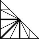
Figure 1.

Proposition 2.17.

For any generic configuration $\mathcal{X}\subset\mathbb{R}^{2}$ of $k=2d+2r-1$ points, $d,r\geq 2$, there exist at least $8$ rational ($\delta-1$)-curves of degree $\Delta_{d,r}$ which pass through the points of $\mathcal{X}$.

Proof.

The proof is similar to the previous proposition. We have $\varkappa(\Delta_{d,r})=2d+2r$ and the infinite directions are either horizontal or vertical, so the maximal contribution of the only $\delta$-curve for any generic configuration $\mathcal{X}$ to $a_{\delta-1}$ is $2d+2r-6$. In the same time with the help of floor diagrams we can verify that $a_{\delta-1}=2d+2r+2$, which is a special case of the following proposition. ∎

Remark 2.18.

The sharpness of Proposition 2.17 is easy to see for $d=r=2$. As $G(0,\Delta_{2,2}=y+10+y^{-1}$ and the floor diagram $\delta$-curve have two vertices of multiplicity 2, we have eight $(\delta-1)$-curves for any floor decomposed generic configuration $\mathcal{X}$.

Recall (see [3]) that an $h$-transversal polygon is given by the following collection of integer numbers: the length $d_{+}\geq 0$ of the upper side, the length $d_{-}\geq 0$ of the lower side, and two sequences of $d>0$ integer numbers: a non-increasing sequence $d_{l}$ and a non-increasing sequence $d_{r}$ (subject to some additional conditions on these numbers, in particular if $d_{+}=0$ then the last element of $d_{r}$ is always greater than the last element of $d_{l}$).

Proposition 2.19.

Let $\Delta$ be a primitive balanced configuration such that $\Delta^{*}$ is an $h$-transverse polygon that has a lattice point in its interior. We have

$$a_{\delta-1}=\varkappa(\Delta)-2+c_{+}(\Delta)+c_{-}(\Delta)+c_{l}(\Delta)+c_{r}(\Delta).$$

for the coefficients $a_{\delta-1}$ of $G(0,\Delta)$ at $y^{\delta(0,\Delta)-1}$.

Here $c_{\pm}=2$ if $d_{\pm}>0$. We have $c_{+}=1$ (resp. $c_{-}=1$) if $d_{+}=0$ (resp. $d_{-}=0$) and the difference between the last elements of $d_{r}$ and $d_{l}$ is 1 (resp. the difference between the first elements of $d_{l}$ and $d_{r}$ is 1). Otherwise $c_{\pm}=0$. We define $c_{l}$ (resp. $c_{r}$) as the number of pairs of subsequent elements in the non-increasing sequence $d_{l}$ (resp. non-increasing sequence $d_{r}$) that are different by 1. In particular, we have $a_{\delta-1}\geq\varkappa(\Delta)-2$.

Proof.

We use the floor decomposition from [3]. If $d_{+}>0$ and $d_{-}>0$ then the contribution of the $\delta$-curve to $a_{\delta-1}$ is $2d-2$ as all its finite elevators must have weight at least 2. There are two possible floor diagrams for a $(\delta-1)$-curve, they have $d_{+}+2$ and $d_{-}+2$ possible markings respectively. Adding up we get $a_{\delta-1}=2d-2+d_{+}+2+d_{-}+2=\varkappa(\Delta)+2$ as $\varkappa(\Delta)=d_{+}+d_{-}+2d$.

If $d_{+}=0$ the top elevator of the $\delta$-curve floor diagram may or may not have weight 1. Its weight is equal to the difference of last elements in $d_{r}$ and $d_{l}$. If this weight is 1 then we have a unique $(\delta-1)$-curve floor diagram with an elevator crossing the second floor from above. In the same time the contribution of the $\delta$-curve to $a_{\delta-1}$ has to be decreased by 2 in such case (in comparison with $2d-2$ in the case when all $(d-1)$ finite elevators have weight at least 2). If this weight is 2 then there is no correction neither to the contribution of the $\delta$-curve nor to the number of $(\delta-1)$-curves. We have a similar situation for the case $d_{-}=0$. ∎

Example 2.20.

If $\Delta=\Delta_{d}$ we have a lattice point in the interior of $\Delta^{*}$ iff $d\geq 3$. In this case we have

$$a_{\delta-1}=3d+1=\varkappa(\Delta)+1.$$

If $\Delta=\Delta_{d,r}$ we have a lattice point in the interior of $\Delta^{*}$ iff $d,r\geq 2$. In this case we have

$$a_{\delta-1}=2d+2r+2=\varkappa(\Delta)+2.$$

If $\Delta^{*}$ is a general $h$-transverse polygon, the argument from the proofs of Proposition 2.15 and 2.17 that ensures two multiplicity 1 vertices for a $\delta$-curve is not applicable. But the contribution of the $\delta$-curve to $a_{\delta-1}$ can still be bounded from above by $\varkappa(\Delta)-2$, the number of all vertices of a rational curve with $\varkappa$ tails. Thus we get the following corollary.

Corollary 2.21.

Let $\Delta$ be a primitive balanced configuration such that $\Delta^{*}$ is an $h$-transverse polygon that has a lattice point in its interior. For any generic configuration $\mathcal{X}$ of $\varkappa(\Delta)-1$ points in $\mathbb{R}^{2}$ there exist at least $c_{+}(\Delta)+c_{-}(\Delta)+c_{l}(\Delta)+c_{r}(\Delta)$ distinct $(\delta-1)$ rational curves through $\mathcal{X}$, where $c_{\pm}$, $c_{r}$ and $c_{l}$ are defined in Proposition 2.19.

Remark 2.22.

For any non-negative integer $j$, we may treat the coefficient of the polynomial $G(g,\Delta)$ at $y^{j}$ as a non-negative integer invariant $a_{j}(g,\Delta)$ for the number of tropical curves passing through a generic configuration of $k=\varkappa(\Delta)+g-1$ points. Here only tropical curves of multiplicity at least $2j+1$ contribute to $a_{j}(g,\Delta)$ (each with the corresponding coefficient at $y^{j}$ of its Block-Göttsche multiplicity). Thus $G(g,\Delta)$ can be viewed as infinite number of integer-valued invariants of tropical curves.

3. Proof of Theorem 1

The second part of the statement follows from Theorem 6 of [15]. The fact that $G(g,\Delta)$ is a symmetric Laurent polynomial with positive coefficients immediately follows from the definition. It remains to prove that $G(g,\Delta)$ is independent on the choice of $\mathcal{X}$. Our proof is similar to the proof of Theorem 4.8 in [7] and the proof of Theorem 1 in [10].

Recall that $\mathcal{X}=\{p_{1},\dots,p_{k}\}$ is a configuration of $k=\varkappa(\Delta)+g-1$ points in $\mathbb{R}^{2}$ tropically generic in the sense of Definition 4.7 of [15]. To show independence of $G(g,\Delta)$ of $\mathcal{X}$ it suffices to show that the sum (2.2) stays invariant if we move one of the points of $\mathcal{X}$, say $p_{k}$ in a smooth path $p_{k}(t)$, $t\in[-\epsilon,\epsilon]$, $\epsilon>0$, so that the configurations $\mathcal{X}(t)=\{p_{1},\dots,p_{k-1},p_{k}(t)\}$ are tropically generic whenever $t\neq 0$.

Let $t_{0}\in[-\epsilon,\epsilon]$, and let $h(t_{0}):C(t_{0})\to\mathbb{R}^{2}$ be a tropical curve of genus $g^{\prime}\leq g$ and degree $\Delta$ such that $\mathcal{X}(t_{0})\subset h(t_{0})(C(t_{0}))$. Put

(3.1) $$\operatorname{def}(C(t_{0}))=\sum_{V}(\operatorname{val}(V)-3)+(g-g^{\prime})+m,$$

where the first sum is taken over all vertices of $C(t_{0})$, and $m$ is equal to the number of vertices of $C(t_{0})$ whose images under $h(t_{0})$ are contained in $\mathcal{X}(t_{0})$.

As $\mathcal{X}(t_{0})$ is tropically generic in the case $t_{0}\neq 0$, it follows from Proposition 2.23 of [15] that $\operatorname{def}(C(t_{0}))=0$. Furthermore, if we slightly perturb our generic points $p_{1},\dots,p_{k-1}\in\mathbb{R}^{2}$ the sets $\mathcal{S}(g,\Delta,\mathcal{X}(\pm\epsilon))$ remain unchanged after perturbation. Proposition 3.9 of [7] implies the following statement.

Lemma 3.1.

There exists a finite set $D\subset\mathbb{R}^{2}$ such that under the condition $p_{k}(t_{0})\not\in D$ one has either $\operatorname{def}(C(t_{0}))\leq 1$, or $\operatorname{def}(C(t_{0}))=2$ and $C(t_{0})$ has two $4$-valent vertices connected by two edges.

Proof.

Proposition 3.9 of [7] concerns the dimensions of the moduli spaces ${\mathcal{M}}_{g,\Delta}^{\alpha}$, of tropical curves $h:C\to\mathbb{R}^{2}$ of genus $g^{\prime}\leq g$ and degree $\Delta$ with $k$ marked points $y_{1},\dots,y_{k}\in C$ such that $(h,y_{1},\ldots,y_{k})$ has a combinatorial type $\alpha$. Here, by the combinatorial type of $(h,y_{1},\dots,y_{k})$, we mean the combinatorial type of the graph $C$ together with the slopes of its edges under $h$ and the distribution of the points $y_{1},\dots,y_{k}$ among the edges and vertices of $C$.

We are looking at the curves $h:C\to\mathbb{R}^{2}$ such that $h(y_{j})=p_{j}$, $j=1,\dots,k$. For a given combinatorial type $\alpha$, consider the evaluation map

$$\operatorname{ev}{\mathcal{M}}_{g,\Delta}^{\alpha}\to(\mathbb{R}^{2})^{k}$$

defined by $(h,y_{1},\dots,y_{k})\mapsto(h(y_{1}),\dots,h(y_{k}))$. As we may slightly perturb our generic points $p_{j}$, $j=1,\dots,k-1$, if needed, we may assume that $\operatorname{ev}^{-1}((p_{1},\dots,p_{k-1})\times\mathbb{R}^{2})$ is of codimension $2k-2$ in ${\mathcal{M}}_{g,\Delta}^{\alpha}$. Thus, any curve $h:C\to\mathbb{R}^{2}$ with $h(y_{j})=p_{j}$, $j=1$, $\ldots$, $k$, must be of a combinatorial type $\alpha$ with $\dim{\mathcal{M}}_{g,\Delta}^{\alpha}\geq 2k-2$. Furthermore, each $\alpha$ with $\dim{\mathcal{M}}_{g,\Delta}^{\alpha}=2k-2$ has a most one (by convexity) value $p_{k}$ admitting such $h$. There are only finitely many distinct combinatorial types. Thus away from a finite set $D\subset\mathbb{R}^{2}$ we only encounter combinatorial types $\alpha$ with $\dim{\mathcal{M}}_{g,\Delta}^{\alpha}>2k-2$ and they are explicitly described by Proposition 3.9 of [7]. ∎

By Lemma 3.1 we may assume that the path $\mathcal{X}(t)$, $t\in[-\epsilon,\epsilon]$, is such that for any curve $h(t_{0}):C(t_{0})\to\mathbb{R}^{2}$ of degree $\Delta$ and genus $g^{\prime}\leq g$ passing through $\mathcal{X}(t)$ we have $\operatorname{def}(C)\leq 2$. In addition, we have $\operatorname{def}(C(t_{0}))=0$ whenever $t_{0}\neq 0$ and $\operatorname{def}(C(0))\leq 1$ unless $C(0)$ has two 4-valent vertices connected by two edges.

Suppose that $h(\epsilon):C(\epsilon)\to\mathbb{R}^{2}$ is a curve passing through $\mathcal{X}(\epsilon)$. When we change $t$ from $\epsilon$ to $0$ the configuration $\mathcal{X}(t)$ moves as well in the class of generic configurations. This uniquely defines a continuous deformation $h(t):C(t)\to\mathbb{R}^{2}$ as by Lemma 4.20 of [15] every connected component $T(\epsilon)\subset C(\epsilon)\smallsetminus h^{-1}(\mathcal{X}(\epsilon))$ is a 3-valent tree with a single leaf going to infinity. All the other leaves of $h(T(\epsilon))$ are adjacent to some points of $\mathcal{X}(\epsilon)$.

Thus one can reconstruct $h(t):C(t)\to\mathbb{R}^{2}$, $0<t<\epsilon$, by tracing the change of $h(T(\epsilon))$ for each such component $T(\epsilon)$. We do it inductively. If $T(\epsilon)$ is a tree without 3-valent vertices then $h(T(\epsilon))$ is an open ray adjacent to $p_{j}(\epsilon)$. If $j<k$ this point does not move and $T(\epsilon)$ remains constant under the deformation. If $j=k$, then $h(T(\epsilon))$ deforms to a parallel ray emanating from $p_{k}(t)$.

Suppose that $T(\epsilon)$ contains 3-valent vertices. Unless $h(T(\epsilon))$ is adjacent to $p_{k}(\epsilon)$, it remains constant under deformation as its endpoints do not move. Let $E(\epsilon)$ be the edge of $T(\epsilon)$ connecting $p_{k}(\epsilon)$ to a 3-valent vertex $v\in T(\epsilon)$. The complement $T(\epsilon)\smallsetminus\{v\}$ consists of three components: the edge $E(\epsilon)$ and two other components $T_{0}(\epsilon)$ and $T_{\infty}(\epsilon)$, where $T_{\infty}(\epsilon)$ is chosen so that it contains the infinite edge leaf.

Let $E_{0}(\epsilon)$ be the edge of $T_{0}(\epsilon)$ adjacent to $v$. The line parallel to $E(\epsilon)$ passing through $p_{k}(t)$ intersects the line containing $E_{0}(\epsilon)$ at a point $v(t)$. If $t<\epsilon$ is sufficiently close to $\epsilon$ then $v(t)$ is sufficiently close to $v$. We form $h(T(t))$ by taking the union of the interval connecting $p_{k}(t)$ to $v(t)$ and the tree obtained by modifying $T_{0}(\epsilon)$ by enlarging or decreasing its leaf edge adjacent to $v(\epsilon)$ so that $h(t)(T_{0}(t))$ is adjacent to $v(t)$. Then we modify the component $T_{\infty}(\epsilon)$ inductively by treating the vertex $v(\epsilon)$ as the marked endpoint for this tree, see Figure 2.

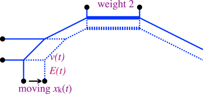
Figure 2. Deformation of $T(\epsilon)$

Note that we may continue this deformation $h(t):C(t)\to\mathbb{R}^{2}$ for any value of $t$, $0<t<\epsilon$. Indeed, the set of $t\in(0,\epsilon]$ for which such a deformation exists is an open neighborhood of $\epsilon$. Let $t_{\inf}$ be the infimum of this set. When $t\to t_{\inf}^{+}$ we get the limiting tree $h(T(t_{\inf}^{+}))$ for each component $T(\epsilon)\subset C(\epsilon)\smallsetminus h^{-1}(\mathcal{X}(\epsilon))$. This tree is a degeneration of the combinatorial type of $T(\epsilon)$ as the length of the edges of $T(\epsilon)$ changes and some values in the limit $t\to t_{\inf}^{+}$ might become zero.

Note that if a length of an edge of $T(\epsilon)$ vanishes then either two or more trivalent vertices collide to a vertex of higher valence or one of the 3-valent vertex collides with a point of $X(t_{\inf}^{+})$. We may combine a limiting curve $h(t_{\inf}^{+}):C(t_{\inf}^{+})\to\mathbb{R}^{2}$ by taking the union of the limiting trees for all such component. Note that the degree of the limiting curve is still $\Delta$ as the number and direction of the infinite rays do not change.

Lemma 3.2.

The genus of $C(t_{\inf}^{+})$ is $g$.

Proof.

The genus of limiting curve may only decrease if the length of all edges in a cycle of $C(\epsilon)$ will simultaneously vanish. This is not possible by Lemma 3.1 as our path for $p_{k}(t)$ is chosen to avoid the set $D$. ∎

Note that $\operatorname{def}(C(t_{\inf}^{+}))$ coincides with the number of the vanishing edges (for all components of $C(\epsilon)\smallsetminus h^{-1}(\mathcal{X}(\epsilon))$). Thus $t_{\inf}=0$. Similarly we may deform any curve $h(-\epsilon):C(-\epsilon)\to\mathbb{R}^{2}$ from $\mathcal{S}(g,\Delta,\mathcal{X}(-\epsilon))$ to a limiting curve $h(0^{-}):C(0^{-})\to\mathbb{R}^{2}$.

Theorem 1 now follows from the following Lemma.

Lemma 3.3.

For each immersed tropical curve $h:C\to\mathbb{R}^{2}$ such that $\mathcal{X}(0)\subset h(C)$, we have

(3.2) $$\sum G(h^{+}_{j})=\sum G(h^{-}_{j})$$

where $h^{\pm}_{j}$ runs over all curves $\mathcal{S}(g,\Delta,\mathcal{X}(\pm\epsilon))$ such that the limiting curve $h^{\pm}_{j}(0^{\pm})$ coincides with $h$.

Proof.

By Lemma 3.2 we may assume that the genus of $C$ is $g$ as otherwise the sums in both sides of (3.2) are empty. By Lemma 3.1 we only need to consider the case when $\operatorname{def}(C)=1$ and the exceptional case of $C$ with two 4-valent vertices connected by two edges.

We assume that $h$ can be presented as the limiting curve of a continuous family $h(t):C(t)\to\mathbb{R}^{2}$, $0<t<\epsilon$ (by changing the parameter $t\mapsto-t$ if needed). First we consider the case when $\operatorname{def}(C)=1$, $C$ is 3-valent and $m=1$ (see (3.1)). In this case we have a 3-valent vertex $v\in C$ such that $h(v)=x_{j}(0)$, for some $j=1,\dots,k$. Accordingly, the length of the segment $E(t)$ connecting $(h(t))^{-1}(p_{j}(t))$ to a 3-valent vertex $v(t)$ in a component $T(t)\subset C(t)\smallsetminus h^{-1}(\mathcal{X}(t))$ must vanish.

Let $A$ be the connected component of $(C\smallsetminus h^{-1}(\mathcal{X}(0)))\cup\{v\}$ that contains the point $v$. Note that $A$ comes as the union of the limits of the family of components $T(t)$ and the family of components $T^{\prime}(t)$ adjacent to $p_{j}(t)$ from the other side, $0<t\leq\epsilon$ (note that $T(t)$ may coincide with $T^{\prime}(t)$ as $T(t)\cup\{p_{j}(t)\}$ does not have to be a tree).

Similarly to the situation we have considered above, the complement $T(t)\smallsetminus\{v(t)\}$ consists of three connected components: $E(t)$, $T_{0}(t)$ and $T_{\infty}(t)$, where $T_{\infty}$ is the component containing the edge going to infinity. Again we denote with $E_{0}(t)$ the edge of $T_{0}(t)$ adjacent to $p_{j}(t)$ (and with $E_{0}(0^{+})$ the limit of this edge when $t\to 0^{+}$). We denote with $E_{\infty}(t)$ the edge of $T_{\infty}(t)$ adjacent to $p_{j}(t)$. Note that while the length of all these edges as well as its position in $\mathbb{R}^{2}$ depend on $t$, their slope remains constant.

Let $L$ be the line extending $E_{0}(0^{+})$. The points $p_{j}(t)$, $t>0$ sit in the same half-plane $H$ bounded by $L$ (since $\mathcal{X}(t)$ is tropically generic whenever $t\neq 0$). If the points $p_{j}(t)$, $t<0$, sit in the same half-plane $H$ then we may extend the family $h(t):C\to\mathbb{R}^{2}$, $0<t\leq\epsilon$, to $-\epsilon<t<0$ keeping the same combinatorial type by the same reconstruction procedure.

Suppose that $p_{j}(t)$ sit in the other half-plane for $t<0$ (note that in such case this holds for all $-\epsilon\leq t<0$). For $t<0$ we define $T_{0}(t)=E^{\prime}(t)\cup T_{0}(0^{+})$, where $E^{\prime}(t)$ is the interval connecting $p_{j}(t)$ to $L$ and parallel to $E_{\infty}(\epsilon)$, see Figure 3. The remaining components of $S\smallsetminus\{v\}$ (as well as those of $C\smallsetminus(S\cup h^{-1}(\mathcal{X}(0)))$) are trees without vanishing edges, so they deform to negative values of $t$ as before.

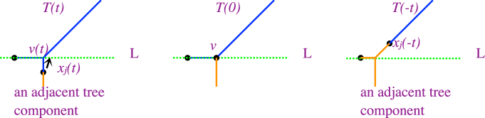
Figure 3. Collision of $v(t)$ and $p_{j}(t)$

This shows that $h$ can be presented as the limiting curve $h(0^{-})$ for a family $h(t)\in\mathcal{S}(g,\Delta,\mathcal{X}(t))$ for $t\in[-\epsilon,0)$. Its combinatorial type is uniquely determined, so by Lemma 4.22 of [15] the family $h(t)$ is unique and both sums in (3.2) consist of a unique term. These terms have the same multiplicity as the curves $h(t):C(t)\to\mathbb{R}^{2}$ for $\pm t>0$ have the same multiplicities for their vertices as the slopes of the corresponding edges are the same (in fact, the only difference of their combinatorial types is in the edge containing $p_{j}(t)$).

Let us now consider the case when $\operatorname{def}(C)=1$, $m=0$ (see (3.1)), and a vertex $v\in C$ is 4-valent. This corresponds to the case when the length of the edge $E(t)\subset C(t)$ connecting two vertices $v(t),v^{\prime}(t)\in C(t)$, $t\in(0,\epsilon]$ vanishes. Consider the component $A$ of $C\smallsetminus h^{-1}(\mathcal{X}(0))$ containing the vertex $v$. This component is a tree since $\operatorname{def}(C)=1$ and thus no edges of $C(t)$, $t\in(0,\epsilon]$, except for $E(t)$ may vanish.

Denote the edges of $C$ adjacent to $v$ with $E_{1}$, $E_{2}$, $E_{3}$ and $E_{\infty}$, so that the order agrees with the counterclockwise order around $h(v)\in\mathbb{R}^{2}$ and $E_{\infty}$ is chosen from the component of $A\smallsetminus v$ containing an edge going to infinity, see Figure 4.

Figure 4. Collision of $v(t)$ and $v^{\prime}(t)$ to a 4-valent vertex.

Each edge $E_{j}$ must come as the limit of an edge $E_{j}(t)$ of the approximating curve $C(t)$. We denote the endpoint of $E_{j}$, $j=1,2,3$, not tending to $h(v)$ by $v_{j}(t)\in C(t)$, $t>0$. (Note that $E_{\infty}$ might not have the other endpoint as it might happen to be an unbounded edge.) The point $h(v_{j}(t))\in\mathbb{R}^{2}$ is inductively determined by $\mathcal{X}(t)$ as well as the slopes of the edges of $C$. These points are thus well-defined also for negative values of $t\in[-\epsilon,\epsilon]$. Denote with $R_{j}(t)$, $j=1,2,3$, the rays emanating from the points $h(v_{j}(t))$ in the direction of the edges $E_{j}(t)$. For $t\neq 0$ these edges cannot intersect in a triple point as $\mathcal{X}(t)$ is generic, but their pairwise intersections must remain close enough to a triple intersection.

If there are no parallel rays among $R_{j}$ we have one of the two types depicted on Figure 5. If the configuration $\mathcal{X}(t)$ for $\pm t>0$ corresponds to the same type of intersection then the combinatorial types of curves from $\mathcal{S}(g,\Delta,\mathcal{X}(\pm\epsilon))$ coincide and both sums in (3.2) are literally the same. Thus we may assume that we have different types of intersections for different signs of $t$.

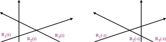
Figure 5. Intersection of rays $R_{1}(t),R_{2}(t),R_{3}(t)$ extending the edges $E_{1}(t),E_{2}(t),E_{3}(t)$.

Possible ways to extend $R_{j}$ to get a 3-valent perturbation of the neighborhood of the 4-valent point $v\in C$ are depicted on Figure 6. We see that we have three possible types for such perturbation. Without loss of generality we may assume that two of them correspond to $t>0$ and one corresponds to $t<0$.

Figure 6. Possible ways to perturb a 4-valent vertex

To compare the contribution of these perturbations to the corresponding sides of (3.2) we consider the dual quadrilateral $Q$ to the vertex $v$, see Definition 2.1. Each type of perturbation of $C$ where a 4-valent vertex $v$ is replaced by two trivalent vertices defines a subdivision of $Q$ into two triangles and, possibly, a parallelogram (which corresponds to the case when there is a self-intersection point of $C(\pm\epsilon)$ near $h(v)$), cf. section 4.1. of [15].

The subdivisions dual to the three possible types of perturbation are shown of Figure 7. Two of these subdivisions are given by drawing diagonals. If the quadrilateral $Q$ does not have parallel sides (i.e. no rays $R_{j}$, $j=1,2,3,\infty$ are parallel) then the third subdivision maybe described as follows. There is a unique parallelogram $P$ such that two of the sides of $P$ coincide with two of the sides of $P$ and $P\subset Q$. The complement $Q\smallsetminus P$ splits into two triangles. Note that the third triangle corresponds to the same sign of $t$ as the subdivision given by the diagonal of $Q$ that also serves as a diagonal of $P$.

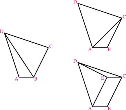
Figure 7. Subdivisions dual to resolving a 4-valent vertex if no adjacent edges are parallel.

We are ready to compute both sides of (3.2) for the case when $Q$ does not have parallel sides. We denote the vertices of $Q$ by $A,B,C,D$ in the counterclockwise order so that the sides $AB$ and $BC$ are also the sides of the parallelogram $P$. Let $E$ be the fourth vertex of $P$. Without loss of generality we may assume that $E$ is inside the (closed) triangle $BCD$ (if $E$ is on the diagonal $AD$ then treat $BDE$ as a degenerate triangle so that $\operatorname{Area}(BDE)=0$).

We have the following straightforward area inequalities: $\operatorname{Area}ACD>\operatorname{Area}ABC$, $\operatorname{Area}BCD)\geq\operatorname{Area}ABD$ and $\operatorname{Area}ADE\geq\operatorname{Area}CDE$. In the last two inequalities we have equalities if and only if the triangle $BDE$ is degenerate.

In the right-hand side of (3.2) we have a single term proportional to

$$(y^{\operatorname{Area}BCD}-y^{-\operatorname{Area}BCD})(y^{\operatorname{Area}ABD}-y^{-\operatorname{Area}ABD})=$$

$$y^{\operatorname{Area}Q}-y^{\operatorname{Area}BCD-\operatorname{Area}ABD}-y^{-\operatorname{Area}BCD+\operatorname{Area}ABD}+y^{-\operatorname{Area}Q}.$$

The proportionality coefficient here is the product of Block-Göttsche multiplicities of all other vertices of $C$ divided by $(y^{\frac{1}{2}}-y^{-\frac{1}{2}})^{2}$. The left-hand side of (3.2) is the sum of two terms:

$$(y^{\operatorname{Area}ACD}-y^{-\operatorname{Area}ACD})(y^{\operatorname{Area}ABC}-y^{-\operatorname{Area}ABC})=$$

$$y^{\operatorname{Area}Q}-y^{\operatorname{Area}ACD-\operatorname{Area}ABC}-y^{-\operatorname{Area}ACD+\operatorname{Area}ABC}+y^{-\operatorname{Area}Q}$$

and

$$(y^{\operatorname{Area}ADE}-y^{-\operatorname{Area}ADE})(y^{\operatorname{Area}CDE}-y^{-\operatorname{Area}CDE})=y^{\operatorname{Area}ADE+\operatorname{Area}CDE}$$

$$-y^{\operatorname{Area}ADE-\operatorname{Area}CDE}-y^{-\operatorname{Area}ADE+\operatorname{Area}CDE}+y^{-\operatorname{Area}ADE-\operatorname{Area}CDE}$$

with the same proportionality coefficient. The terms $y^{\operatorname{Area}Q}+y^{-\operatorname{Area}Q}$ in both sides annihilate. Furthermore we have a simplification after adding the two terms of the left-hand side as

$$\operatorname{Area}ACD-\operatorname{Area}ABC=\operatorname{Area}Q-\operatorname{Area}P=\operatorname{Area}ADE+\operatorname{Area}CDE.$$

We are left with $-y^{\operatorname{Area}BCD-\operatorname{Area}ABD}-y^{-\operatorname{Area}BCD+\operatorname{Area}ABD}$ in the right-hand side and with $-y^{\operatorname{Area}ADE-\operatorname{Area}CDE}-y^{-\operatorname{Area}ADE+\operatorname{Area}CDE}$. Thus to finish the proof in the case when $Q$ is not a trapezoid it suffices to show that $\operatorname{Area}BCD-\operatorname{Area}ABD=\operatorname{Area}ADE-\operatorname{Area}CDE$. However, since $P=ABCE$ is a parallelogram we have

$$\operatorname{Area}BCD-\operatorname{Area}ADE=\operatorname{Area}P=\operatorname{Area}ABD-\operatorname{Area}CDE.$$

Let us now consider the case when some of the edges $E_{1},E_{2},E_{3},E_{\infty}$ are parallel. Note that in this case only two of them may be parallel to the same direction. Indeed, by the balancing condition if three edges are parallel then the fourth edge must also be parallel to them. But in this case $v$ is the result of colliding of two 3-valent vertices of $C(t)$ where the map $h(t)$ cannot be an immersion. Thus either we have exactly two edges that are parallel or we have two pairs of parallel edges.

Suppose that two edges are not only parallel, but emanate from $v$ in the same direction. By the balancing condition two other edges cannot be parallel. If one of the two parallel edges is $E_{\infty}$ then no two rays among $R_{1}(t),R_{2}(t),R_{3}(t)$ are parallel. So, once again we have one of the two ways to perturb a triple point of intersections of these rays (cf. Figure 5). If the pair of parallel edges is disjoint from $E_{\infty}$ then there are still two possibilities for the rays $R_{1}(t)R_{2}(t),R_{3}(t)$ as the parallel rays may be perturbed in two different ways.

In any of these cases the dual polygon $Q$ in this case is a triangle. Furthermore any nearby configuration of $R_{1}(t),R_{2}(t),R_{3}(t)$ corresponds to a unique subdivision of the triangle $Q$ into triangles so that the new vertex of the subdivision is contained in the side dual to the pair of parallel edges and subdivides them into the intervals of integer lengths corresponding to the weights of the parallel edges. The only possible difference is the order of these intervals in $\partial Q$. The unordered pair formed by the areas of the triangles of the subdivision is the same, thus the corresponding Block-Göttsche multiplicities are also the same.

If there are no edges among $E_{1},E_{2},E_{3},E_{\infty}$ emanating in the same direction, but there are parallel edges then $Q$ is a trapezoid (possibly a parallelogram as we may have two pairs of parallel edges in this case). Then there is a unique way to reconstruct a perturbation of $h:C\to\mathbb{R}^{2}$ for each of the two cases of Figure 5 as the combinatorial type of one of the perturbations (the one with a self-intersection point) has a 3-valent vertex with all three adjacent edges parallel to the same direction. This combinatorial type cannot be realized by an immersion and thus does not appear for a generic configuration of points $\mathcal{X}(t)$, $t\neq 0$.

Thus if $Q=ABCD$ is a trapezoid (say $AB$ and $CD$ are parallel sides) we have the contribution of $y^{\operatorname{Area}Q}-y^{\operatorname{Area}BCD-\operatorname{Area}ABD}-y^{-\operatorname{Area}BCD+\operatorname{Area}ABD}+y^{-\operatorname{Area}Q}$ and of $y^{\operatorname{Area}Q}-y^{\operatorname{Area}ACD-\operatorname{Area}ABC}-y^{-\operatorname{Area}ACD+\operatorname{Area}ABC}+y^{-\operatorname{Area}Q}$ on the different side of (3.2). But $\operatorname{Area}BCD=\operatorname{Area}ACD$ while $\operatorname{Area}ABC=\operatorname{Area}ABD$ since $AB$ and $BC$ are parallel, so the contributions are the same.

Finally we have to consider the case when $\operatorname{def}(C)=2$. Let $v,v^{\prime}\in C$ be two 4-valent vertices connected by two edges $E,E^{\prime}\subset C$. Note that by Lemma 3.1 the vertices of $C$ are disjoint from $\mathcal{X}(0)$. We claim that if $h:C\to\mathbb{R}^{2}$ can be presented as a limiting curve $h(0^{\pm})$ for $h(t)\in\mathcal{S}(g,\Delta,\mathcal{X}(t))$, $\pm t>0$, then $h(E\cup E^{\prime})\cap\mathcal{X}(0)\neq\emptyset$. Indeed, the union $E\cup E^{\prime}$ forms a cycle in $C$ and if it is disjoint from $\mathcal{X}(0)$ it must remain disjoint from $\mathcal{X}(t)$ after a perturbation which contradicts to our hypothesis that $\mathcal{X}(t)$, $t\neq 0$, is generic by Lemma 4.20 of [15].

On the other hand the set $h(E\cup E^{\prime})\cap\mathcal{X}(0)$ cannot have more than two points as each edge of $C(t)$, $t\neq 0$, can hit no more than one point of $\mathcal{X}(t)$. If we have two points $p_{j}(0),p_{j^{\prime}}(0)\in h(E\cup E^{\prime})\cap\mathcal{X}(0)$ then they must come from different edges of the approximating curve, i.e. $p_{j}(t)\in E(t)$ and $p_{j^{\prime}}(t)\in E^{\prime}(t)$, where $E(t),E^{\prime}(t)\subset C(t)$ are the edges limiting at $E$ and $E^{\prime}$.

The (common) endpoints $v(t),v^{\prime}(t)$ of $E(t)$ and $E^{\prime}(t^{\prime})$ belong to two different tree components $T(t)$ and $T^{\prime}(t)$ of $C\smallsetminus h(t)^{-1}(\mathcal{X}(t))$. These trees have one vanishing edge each (corresponding to $v$ and $v^{\prime}$ respectively). There is a unique tree approximating $T(0^{\pm})$ (resp. $T^{\prime}(0^{\pm})$) for any generic perturbation of the configuration $\mathcal{X}(0)$. The only possible difference in the resulting combinatorial type is the exchange of $p_{j}(t)$ and $p_{j^{\prime}}(t)$ on $E(t)$ and $E^{\prime}(t)$. It does not affect the slopes of the edges and thus the multiplicity of the curves.

If $h(E(t))\ni p_{j}(t)$ but $h(E^{\prime}(t))\cap\mathcal{X}(t)=\emptyset$ then $v(t),v^{\prime}(t)$ belong to the same component $T(t)$ of $C\smallsetminus h(t)^{-1}(\mathcal{X}(t))$ and this component has two disjoint vanishing edges. Let $T\subset C$ be the limit of $T(t)$ when $t\to 0^{\pm}$. Suppose the unbounded edge of $T$ belongs to the component of $T\smallsetminus\{v,v^{\prime}\}$ adjacent to $v^{\prime}$.

We may treat the vanishing edges one by one. First we consider the perturbation of the vertex $v$, where the position of the lines containing the results of perturbation of three out of four adjacent edges (all except for $E^{\prime}$) are inductively determined by $\mathcal{X}(t)$ and the slopes of the combinatorial type. In its turn, the combinatorial type of the perturbation near $v$ is unique as two edges of $C$ adjacent to $v$ emanate in the same direction.

This determines both trivalent vertices that approximate $v$ as well as the line containing $E(t)$. We proceed with the perturbation of $v^{\prime}$ in the same way. Once again we get that there is a unique combinatorial type of $h(t)\in\mathcal{S}(g,\Delta,\mathcal{X}(t))$ approximating $h$ for each generic perturbation $\mathcal{X}(t)$ of $\mathcal{X}(0)$ and it multiplicity does not depend on the choice of perturbation. ∎

References

- [1] Florian Block and Lothar Göttsche. In preparation.
- [2] Erwan Brugallé and Grigory Mikhalkin. Enumeration of curves via floor diagrams. C. R. Math. Acad. Sci. Paris, 345(6):329–334, 2007.
- [3] Erwan Brugallé and Grigory Mikhalkin. Floor decomposition of tropical curves: the planar case. Proceedings of 15th Gökova Geometry-Topology Conference, pages 64–90, 2008.
- [4] L. Caporaso and J. Harris. Counting plane curves of any genus. Invent. Math., 131(2):345 392, 1998.
- [5] A. Degtyarev and V. Kharlamov. Topological properties of real algebraic varieties: Rokhlin’s way. Russian Math. Surveys, 55(4):735–814, 2000.
- [6] Sergey Fomin and Grigory Mikhalkin. Labeled floor diagrams for plane curves. J. Eur. Math. Soc. (JEMS), 12(6):1453–1496, 2010.
- [7] Andreas Gathmann and Hannah Markwig. The numbers of tropical plane curves through points in general position. J. Reine Angew. Math., 602:155–177, 2007.
- [8] Lothar Göttsche and Vivek Shende. In preparation.
- [9] Ilia Itenberg, Viatcheslav Kharlamov, and Eugenii Shustin. Welschinger invariant and enumeration of real rational curves. Int. Math. Res. Not., (49):2639–2653, 2003.
- [10] Ilia Itenberg, Viatcheslav Kharlamov, and Eugenii Shustin. A Caporaso-Harris type formula for Welschinger invariants of real toric del Pezzo surfaces. Comment. Math. Helv., 84(1):87–126, 2009.
- [11] M. Kontsevich and Yu. Manin. Gromov-Witten classes, quantum cohomology, and enumerative geometry. Comm. Math. Phys., 164(3):525–562, 1994.
- [12] M. Kool, V. Shende, and R. P. Thomas. A short proof of the Göttsche conjecture. Geom. Topol., 15:397–406, 2011.
- [13] Grigory Mikhalkin. Enumeration of real algebraic curves in the plane and tropical folding of relevant caustics. To appear.
- [14] Grigory Mikhalkin. Counting curves via lattice paths in polygons. C. R. Math. Acad. Sci. Paris, 336(8):629–634, 2003.
- [15] Grigory Mikhalkin. Enumerative tropical algebraic geometry in . J. Amer. Math. Soc., 18(2):313–377, 2005.
- [16] Grigory Mikhalkin. Tropical geometry and its applications. In International Congress of Mathematicians. Vol. II, pages 827–852. Eur. Math. Soc., Zürich, 2006.
- [17] Grigory Mikhalkin. Informal discussion: Enumeration of real elliptic curves. Oberwolfach Reports, (20):44–47, 2011.
- [18] Grigory Mikhalkin and Ilia Zharkov. Tropical curves, their Jacobians and theta functions. In Curves and abelian varieties, volume 465 of Contemp. Math., pages 203–230. Amer. Math. Soc., Providence, RI, 2008.
- [19] Jean-Yves Welschinger. Invariants of real symplectic 4-manifolds and lower bounds in real enumerative geometry. Invent. Math., 162(1):195–234, 2005.