Free path lengths in quasi crystals

Abstract.

The Lorentz gas is a model for a cloud of point particles (electrons) in a distribution of scatterers in space. The scatterers are often assumed to be spherical with a fixed diameter $d$, and the point particles move with constant velocity between the scatterers, and are specularly reflected when hitting a scatterer. There is no interaction between point particles. An interesting question concerns the distribution of free path lengths, i.e. the distance a point particle moves between the scattering events, and how this distribution scales with scatterer diameter, scatterer density and the distribution of the scatterers. It is by now well known that in the so-called Boltzmann-Grad limit, a Poisson distribution of scatters leads to an exponential distribution of free path lengths, whereas if the scatterer distribution is periodic, the distribution of free path behaves asymptotically like a Cauchy distribution.

This paper considers the case when the scatters are distributed on a quasi crystal, i.e. non periodically, but with a long range order. Simulations of a one-dimensional model are presented, showing that the quasi crystal behaves very much like a periodic crystal, and in particular, the distribution of free path lengths is not exponential.

1. Introduction

The Lorentz gas is a mathematical model for the motion of (point) particles in e.g. a crystal, consisting of spherical, elastic scatterers of radius $a$ with centers at a fixed set of points $\Gamma_{\varepsilon}\subset\mathbb{R}^{n}$. A point particle moves in straight lines between the obstacles, on which it is specularly reflected. At least two very different scatterer distributions, $\Gamma_{\varepsilon}$ have been studied thoroughly: the standard lattice ${\mathcal{L}}\subset\mathbb{R}^{n}$, with interstitial distance $\varepsilon^{(n-1)/n}$, or a random distribution, where $\Gamma_{\varepsilon}$ is Poisson distributed with intensity $\varepsilon^{-(n-1)}$. In this paper we are mainly concerned with the so called Boltzmann-Grad limit of this system, and that corresponds to setting the scatter radius $a=\varepsilon$ and letting $\varepsilon\rightarrow 0$. Very loosely speaking, in this scaling the mean free path of the point particles remain of order one as $\varepsilon\rightarrow 0$. Consider now a density $f_{\varepsilon}(x,v,t]$ of point particles moving between the scatterers. Gallavotti [9] (see also [10]) considered the random obstacle distribution, and proved that when $\varepsilon\rightarrow 0$, $f_{\varepsilon}(x,v,t)$ converges to a function that solves a linear Boltzmann equation. On the other hand, Golse [11] proved, based on results in [3] and [12], that in the periodic case, the limiting particle distribution does not satisfy a linear Boltzmann equation. Caglioti and Golse [6, 7, 8] and Marklof and Strömbergsson [15, 16, 17, 18] independently found sharp estimates of the distribution of free path lengths and that the Boltzmann-Grad limit corresponds to a Boltzmann like equation in an extended phases space that does describe the evolution of a particle density in the limit of small $\varepsilon$; whereas the results in [6, 7, 8] are restricted to two space dimensions and rely on an independence assumption, [15, 16, 17, 18] provides a complete proof valid for any space dimension. Related results valid for in the two-dimensional case, can be found in [2, 1], and in [4]. Situations where scatterers are randomly place on a periodic lattice have been considered in  [5] and  [20].

Here we are interested in the case where the obstacles are distributed as the atoms in a quasi crystal. By definition a crystal is ”a solid with an essentially discrete diffraction pattern” [21]. It has been known for a long time that periodic crystals in three dimensions must belong to one of fourteen symmetry classes. A quasi crystal is a crystal whose diffraction pattern exhibits a forbidden symmetry. The first reports on experimental results indicating that such solids exist were treated with suspicion by the scientific community, but in 2011 their discovery was awarded the Nobel Prize in Chemistry [13].There are also many mathematical abstract constructions that give the same results, starting e.g. from the Penrose tiling (see e.g. [21]). It is then a natural question to ask whether the Boltzmann-Grad limit of a Lorentz gas in a quasi crystal behaves more like the random or periodic case. In this paper we present simulation results on a one-dimensional model, which give strong support for the latter: the free path length distribution decays polynomially, just as in the periodic case, whereas in the random case, the path length distribution is exponentially decaying.

The next section gives precise definitions of the Lorentz model, and of its Boltzmann-Grad limit, and some results concerning the periodic and random cases are discussed. Thereafter, in Section 3, a construction of quasi crystals is given; that section is mainly based on [21].

Section 4 presents the simulation method and the results, and the paper ends with conclusions and some prospects for future research in Section 5.

2. Free path length distributions in the Lorentz model

The discussion in this section is restricted to the Lorentz gas in two dimensions, and hence we consider a point distribution $\Gamma_{\varepsilon}\subset\mathbb{R}^{2}$, or more precisely, a family of point distributions parametrized by $\varepsilon$. At each point $p\in\Gamma_{\varepsilon}$ we put a circular obstacle with radius $\varepsilon$ and center at $p$, and then we study the motion of a point particle moving with constant speed, $|\mathbf{v}|=1$, along straight lines between the obstacles, and specularly reflected when hitting an obstacle. Hence the phase space for one point particle is $\Omega_{\Gamma_{\varepsilon}}\times S^{1}$, where

$$\Omega_{\Gamma_{\varepsilon}}=\mathbb{R}^{2}\setminus\bigcup_{p\in\Gamma}\bar{B}_{p}(\varepsilon)$$

and $\bar{B}_{p}(\varepsilon)$ is the closed ball of radius $\varepsilon$ centered at $p\in\mathbb{R}^{2}$. For any initial point $(x_{0},v_{0})$ we define

$$T_{\Gamma_{\varepsilon}}^{t}(x_{0},v_{0})=(x(t),v(t))\,,$$

the position of the point particle at time $t$, taking into account all reflections on the set of obstacles. As long as the obstacles do not overlap, this is well defined for all $t\geq 0$. Moreover, the the free path length is defined as

$$\tau_{\varepsilon}(x_{0},v_{0})=\inf\left\{t>0\,\Big{|}\,x_{0}+tv_{0}\notin\Omega_{\Gamma_{\varepsilon}}\right\}\,.$$

We also define the path length distribution

(1) $$\phi_{\varepsilon}(]a,b[)=\lim_{R\rightarrow\infty}\frac{m(\{(x,v)\in\left(\Omega_{\Gamma_{\varepsilon}}\cap B_{0}(R)\right)\times S^{1}\,|\,\tau_{\varepsilon}(x,v)\in]a,b[)\}}{m(\Omega_{\Gamma_{\varepsilon}}\cap B_{0}(R))}\,.$$

Here $m(\cdot)$ is the Lebesgue measure restricted to $\Omega_{\Gamma_{\varepsilon}}\times S^{1}$. In cases where, at least formally, one can prove that for all intervals $[a,b]$, $\phi_{\varepsilon}(]a,b[)$ remains bounded from above and below when $\varepsilon\rightarrow 0$ one speaks of a Boltzmann-Grad limit.

The two typical examples of point distributions $\Gamma_{\varepsilon}$ considered in connection with the Lorentz gas are the periodic distributions $\Gamma_{\varepsilon}=a(\varepsilon)\mathbb{Z}^{2}$, and a Poissonean random distribution with intensity $a(\varepsilon)$.

For a periodic distribution it is more natural to define the free path length distribution by restricting to a lattice unit cell rather than to a ball of radius $R$ as in (1). Of course, in the limit $R\rightarrow\infty$ the result is the same. In this case the Boltzmann-Grad limit corresponds to choosing $a(\varepsilon)=\varepsilon^{1/2}$. The path length distribution $\phi_{\varepsilon}$ in the Boltzmann-Grad limit has been studied in [3, 12], and then, with very sharp bounds in [6, 7, 8] using the theory of continued fractions, and [15, 16, 17, 18] using methods based on Ratner’s theorem. The result is that $\phi_{\varepsilon}([T,\infty[)\rightarrow C\,T^{-1}$ asymptotically for large $T$ when $\varepsilon\rightarrow 0$.

The distribution $\Gamma_{\varepsilon}$ is a Poisson distribution with intensity $a(\varepsilon)$ if and only if for any set $A\subset\mathbb{R}^{2}$,

$${\mathrm{Prob}}\left(\mbox{ no of points in }A=k\right)=\frac{\left(m(A)a(\varepsilon)\right)^{k}}{k!}e^{-m(A)a(\varepsilon)}\,,$$

and in also, for $A\subset\mathbb{R}^{2}$ and $B\subset\mathbb{R}^{2}$ with $A\bigcup B=\emptyset$, the number of points in $\Gamma_{\varepsilon}\bigcup A$ and $\Gamma_{\varepsilon}\bigcup B$ are independent random variables. Here the Boltzmann-Grad limit is achieved by setting $a(\varepsilon)=\varepsilon^{-1}$, and letting $\varepsilon$ go to zero. This distribution differs from the periodic one in several fundamental aspects. First, obstacles may overlap, and hence the trajectories $(x(t),v(t))$ cannot always be continued uniquely. However, the measure of such, bad trajectories goes to zero when $\varepsilon\rightarrow 0$. Secondly, before taking the limit $\mathbb{R}\rightarrow\infty$ in the definition of the path length distribution, the expression in the right hand side of equation (1) is a random variable, but one that converges to a deterministic value both when $R\rightarrow\infty$, and when $\varepsilon\rightarrow 0$. The path length distribution $\phi_{\varepsilon}([T,\infty[)$ converges to a distribution $\phi([T,\infty[)\sim\exp(-cT)$. The Lorentz gas with Poisson distributed obstacles has been studied in detail by Gallavotti [9], who proved that if $f_{\varepsilon,0}(x,v)\in L^{1}\left(\Omega_{\Gamma_{\varepsilon}}\times S^{1}\right)$ are densities of initial points for point particles, and $f_{\varepsilon}(x,v,t)=\mathbb{E}\left[f_{\varepsilon,0}(T^{-t}_{\Gamma_{\varepsilon}}(x,v))\right]$, then, assuming that $f_{\varepsilon,0}\rightarrow f_{0}\in L^{1}(\mathbb{R}^{2}\times S^{1})$, it follows that $f_{\varepsilon}(x,v,t)\rightarrow f(x,v,t)$, which solves a linear Boltzmann equation.

A different class of random distributions of scatterers can be constructed starting from a periodic distribution, by removing obstacles randomly, independently, with some probability $p(\varepsilon)$. Although for a given, positive $\varepsilon$, the behavior is rather different from the Poissonean case, this difference disappears in the limit as $\varepsilon\rightarrow 0$, and in particular, it is possible to rigorously derive a linear Boltzmann equation starting from such distributions (see [5, 20]).

The following section gives examples of mathematical constructions of quasi crystals, and the corresponding Lorentz gas. However, computing long point particle trajectories in a quasi crystal Lorentz gas is very time consuming, and therefore the simulation results presented in this paper are performed on a one-dimensional discrete model. In the two-dimensional periodic case, the path length distribution can be computed almost exactly by analyzing the discrete map given by the consecutive intersections of a trajectory with lines parallel to the lattice containing lattice points, as in Figure 1. We assume here that $a=1$. For an initial point $(x_{0},v)$ with $x_{0}=(q_{0},\tilde{q}_{0})$ sitting on a horizontal line as in the figure, and with $v\in S^{2}$ having an angle $\theta$ to the vertical line, the distance between two consecutive points is $\tan(\theta)$. To find the free path length of a trajectory in a periodic Lorentz gas is then (almost) equivalent to computing

(2) $$k=\min\left\{j\;\big{|}\;\mbox{dist}(q_{j},\mathbb{Z})\leq\sqrt{\varepsilon}/2\right\}.$$

In fact, we will have $\tau_{\varepsilon}(x_{0},v)=\sqrt{\varepsilon}(k\pm 1)/\cos\theta$.

Figure 1. Computing the free path length in a periodic Lorentz gas is equivalent to to a discrete map.

3. Quasi crystals

The material in this section is mostly taken from M. Senechal’s book ”Quasi Crystals and Geometry” [21], which gives a good introduction to the subject.

There are several ways of construction point sets in $\mathbb{R}^{n}$ that satisfy the requirement for being a quasi crystal: ”an essentially discrete diffraction pattern exhibiting a forbidden symmetry”. One of these is the so called projection method:

• Let ${\mathcal{L}}^{p}$ be a point lattice in $\mathbb{R}^{k}$ (usually the standard lattice), and let $K$ be the unit cell in the lattice that contains the origin.

• Let $\mathcal{E}$ be an $n$-dimensional subspace of $\mathbb{R}^{k}$, such that $\mathcal{E}\cap{\mathcal{L}}^{p}=\{0\}$, and let $\mathcal{E}^{\perp}$be the orthogonal complement of $\mathcal{E}$.

• Let $\Pi$ and $\Pi^{\perp}$ be the orthogonal projections on $\mathcal{E}$ and $\mathcal{E}^{\perp}$ respectively.

• Let $X={\mathcal{L}}^{p}\cap\left(\Pi^{\perp}(K)\oplus\mathcal{E}\right)$, i.e. the set of lattice points contained in the strip (or cylinder) obtained by translating the unit cell $K$ along $\mathcal{E}$.

The quasi crystal is $\Lambda=\Pi(X)$, the orthogonal projections of $X$ on $\mathcal{E}$. This set is discrete ($\inf\left\{|p_{1}-p_{2}|\;\big{|}\;p_{1},p_{2}\in\Lambda\right\}=r_{0}>0$), non periodic and relatively dense (meaning that there is $R_{0}>0$ such that every sphere in $\mathcal{E}$ of radius greater than $R_{0}$ contains at least one point of $\Lambda$) (see Figure 2). That $\Lambda$ is discrete and relatively dense implies in particular that it is possible to define a scaling that corresponds to the Boltzmann-Grad limit.

The theory of quasi crystals started with the (experimental) discovery of a material exhibiting a five-fold symmetry. Mathematically this can be constructed using the projection method, starting from the regular lattice in $\mathbb{R}^{5}$. A unit cell in this lattice is the hyper cube $Q_{5}$ with 32 vertices

$$\frac{1}{2}\sum_{j=1}^{5}\alpha_{j}e_{j},\qquad,\alpha_{j}\in\{-1,1\}\,$$

where $e_{1}=(1,0,0,0,0),....,e_{5}=(0,0,0,0,1)$. A five fold symmetry is given by cyclic permutation of the unit vectors $e_{j}$, a transformation that can be represented by the rotation matrix

$$\mathcal{A}=\left[\begin{array}[]{ccccc}0&0&0&0&1\\ 1&0&0&0&0\\ 0&1&0&0&0\\ 0&0&1&0&0\\ 0&0&0&1&0\end{array}\right]$$

which by an orthogonal change of variables becomes

$$\left[\begin{array}[]{ccccc}\cos(\frac{2\pi}{5})&-\sin(\frac{2\pi}{5})&0&0&0\\ \sin(\frac{2\pi}{5})&\cos(\frac{2\pi}{5})&0&0&0\\ 0&0&\cos(\frac{4\pi}{5})&-\sin(\frac{4\pi}{5})&0\\ 0&0&\sin(\frac{4\pi}{5})&\cos(\frac{4\pi}{5})&0\\ 0&0&0&0&1\end{array}\right]$$

In these new coordinates, $\mathcal{E}$ will be the subspace spanned by $(1,0,0,0,0)$ and $(0,1,0,0,0)$. The quasi crystal will then be the the set

$$\Pi\left({\mathcal{L}}^{p}\cup\left(\Pi^{\perp}(\mathcal{Q}_{5})\oplus\mathcal{E}\right)\right)\subset\mathcal{E}\,.$$

A one-dimensional quasi crystal can be defined in the similarly as a projection on a one dimensional subspace of $\mathbb{R}^{2}$. Particular examples, which are convenient for numerical computations, are the point sequences known as Fibonacci sequences. They are defined by taking

$$\mathcal{E}=\left\{x\in\mathbb{R}^{2}\,|\,x\cdot\omega=0\right\}\,,$$

where

$$\omega=(-1,\tau)\quad\mbox{with}\quad\tau=\frac{1+\sqrt{5}}{2}\,.$$

Let $\nu=|\omega|=\sqrt{1+\tau^{2}}$. There is an explicit formula for computing the sequence of points that constitute the one-dimensional quasi crystal $\mathcal{F}$ obtained by this construction:

(3) $$\mathcal{F}=\bigcup_{m\in\mathbb{Z}}\{x_{m}\}\quad\mbox{with }\quad x_{m}=\frac{m}{\nu}+\frac{1}{\tau\nu}\left\|\frac{m}{\tau}\right\|\,,$$

where $\|\cdot\|$ denotes the distance to the nearest integer. This sequence has many interesting properties, and in particular it satisfies the criteria that defines a quasi crystal. A particularity is that the interval between two consecutive points are of exactly two kinds, short and long:

$$x_{m}-x_{m-1}=\frac{1}{\nu}\quad\mbox{or}\quad\frac{1}{\nu}+\frac{1}{\nu\tau}\,.$$

As we have seen above, there is a very direct connection between the periodic Lorentz gas in two dimensions and a discrete model, at least when it comes to computing the free path-length distribution, illustrated in Figure 1 and Equation (2). Here we define the rescaled free path length

(4) $$\tau_{\varepsilon}(q_{0},v)=\varepsilon\min\left\{j\;\big{|}\;\mbox{dist}(q_{0}+jv,\mathcal{F})\leq\varepsilon/2\right\}.$$

(Note that compared to Equation (2) the scaling factor $\sqrt{\varepsilon}$ is replaced by $\varepsilon$, the only reason being to make notation more clean).

In the following section we simulate trajectories in order to estimate the path length distribution and compare with simulation results when $\mathcal{F}$ is replaced by $\alpha^{-1}\mathbb{Z}$, and with a Poisson stream of points $x_{j}$ with intensity $\alpha$. The factor $\alpha$ is chosen so that all three point distributions have the same density, asymptotically:

$$\alpha=\lim_{R\rightarrow\infty}\frac{\#([-R,R]\bigcap\mathcal{F})}{2R}=\frac{\tau^{2}}{\nu}\,.$$

This is not equivalent to the free path length distribution in a two-dimensional Lorentz gas as it is in the periodic case, however.

Figure 2. A two dimensional representation of the projection method for constructing quasi crystals

4. Simulation method and results

Here we study the distribution of free path lengths of a point particle jumping on the real line, i.e. the number of jumps needed before the particle falls into an interval of width $\varepsilon$ with center at either the quasi crystal $\mathcal{F}$, as defined previously, the periodic lattice $\frac{\nu}{\tau^{2}}\mathbb{Z}$, or on a Poisson distributed set of points, $\Gamma_{\varepsilon}$ with intensity $\tau^{2}/\nu$. The intensity of the Poisson distribution and the scaling of the periodic lattice are chosen in order that all three obstacle distributions have the same density.

The random starting points $q_{0}$ are chosen randomly, uniformly in the interval
$10000\nu/\tau^{2}$. Obviously, for computing the path length distribution in the random obstacle distribution this is not necessary, $q_{0}=0$ would give exactly the same result. Moreover, in this case the distribution can be computed analytically in the limit of small $\varepsilon$. That case is included in the simulation only for comparison. In the periodic distribution of scatterers it would be more natural to chose a random initial point uniformly in the interval $[0,\nu/\tau^{2}]$, but by definition the quasi crystal is not periodic, and therefore it is natural to chose a larger interval.

For the simulations presented here, $v$ is chosen uniformly in $[0,\nu/\tau^{2}]$. To obtain a result completely equivalent to the periodic Lorentz gas in two dimensions, one should have taken $v=\frac{\nu}{\tau^{2}}\tan\theta$ with $\theta$ uniformly chosen in the interval $[0,\pi/4]$, but simulations with different jump length distributions show give very similar results, and this is not presented here. However, we have only tried distributions with bounded densities.

The position of the point particle after $j$ jumps is denoted $q_{j}=q_{0}+vj$, and the points $x_{m}\in\mathcal{F}$ in the Fibonacci sequence are computed with the formula (3). The points in the Poisson distribution are computed independently for each trajectory $q_{m}$.

The simulation procedure is then

1. Chose $q_{0}$ and $v$ randomly

2. Compute $k_{\mathcal{F},\varepsilon}=\min\left\{j\;\big{|}\;\mbox{dist}(q_{0}+jv,\mathcal{F})\leq\varepsilon/2\right\}$

3. Compute $k_{\mathcal{\mathbb{Z}},\varepsilon}=\min\left\{j\;\big{|}\;\mbox{dist}(q_{0}+jv,\frac{\nu}{\tau^{2}}\mathbb{Z})\leq\varepsilon/2\right\}$

4. Compute $k_{\Gamma,\varepsilon}=\min\left\{j\;\big{|}\;\mbox{dist}(q_{0}+jv,\Gamma)\leq\varepsilon/2\right\}$, where $\Gamma$ is the random obstacle distribution. Note that for a given trajectory $q_{k}$, the free path time is a random variable, depending on the realization of the obstacle distribution. Only one realization of the random obstacle has been chosen.

5. Make a record of each of these path lengths, and repeat a large number $N$ times.

For all simulation results presented below, $N=2\times 10^{7}$, and the results results have been used to estimate $\mathrm{Prob}[k_{*,\varepsilon}\geq K]$, where $*$ represents the different obstacle distributions. In connection with the Lorentz equation, the relevant quantity is the path length distribution expressed in time units, $\mathrm{Prob}[\varepsilon k_{*,\varepsilon}\geq T]$, which is estimated as

(5) $$\phi_{*\varepsilon}([T,\infty[)=\frac{\mbox{Number of trajectories with }k_{*,\varepsilon}\geq T\,\varepsilon^{-1}}{N}$$

The first example, shown in Figure 3, compares the free path length distributions with the three different distribution of scatterers that we consider here for $\varepsilon=10^{-5}$. The graph, plotted in logarithmic scale, show the $1/T$-behavior of $\phi_{*,\varepsilon}([T,\infty[)$ both for the quasi crystal $\mathcal{F}$ and for the periodic distribution, while the random distribution gives a different result (an exponential decay, as expected).

Figure 3. The free path length distribution based on $10^{7}$ trajectories and $\varepsilon=10^{-5}$. The curves show the result for the Fibonacci distribution of scatters (green), the periodic distribution (blue) and the random distribution (magenta).

Figure 4 shows the same as Figure 3 but with $\varepsilon=10^{-4}$ (left) and $\varepsilon=10^{-3}$ (right). Note that the path length distribution for the random obstacle distribution is exponentially only in of the exponential distribution for large $T$. This corresponds the fraction of trajectories with a jump length $v<\varepsilon$ which are stopped by the first obstacle they reach.

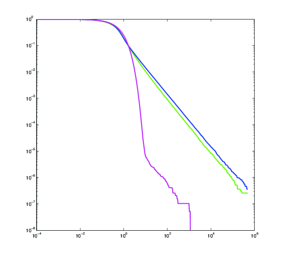
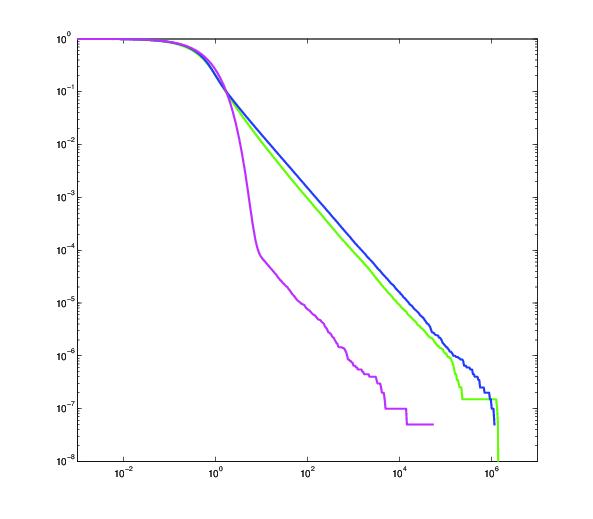
Figure 4. The free path length distribution computed as in Figure 3 but with $\varepsilon=10^{-4}$ (left) and $\varepsilon=10^{-3}$ (right)

Finally, Figure 5 shows the path length distribution $\phi_{\mathcal{F},\varepsilon}([T,\infty[)$ for the quasi crystal with three different values of $\varepsilon$. The graph on the left shows distribution of the number of free steps , $k_{\mathcal{F},\varepsilon}$, and the graph on the right shows the three curves expressed as a function of $T$, as in Equation 5. That these curves almost coincide is a strong indication that $\phi_{\mathcal{F},\varepsilon}[T,\infty[)$ converges to some distribution $\phi_{\mathcal{F}}[T,\infty[)$ as $\varepsilon\rightarrow\infty$, just as in the periodic case.

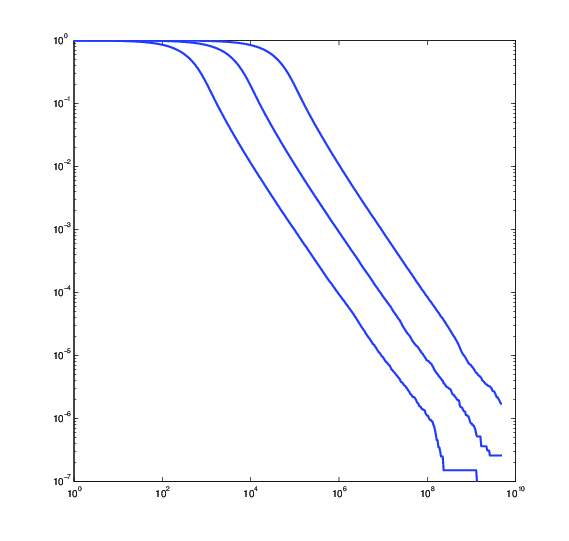
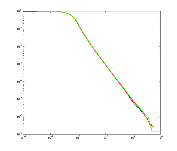
Figure 5. The free path length distribution in the quasi crystal, for $\varepsilon=10^{-5},10^{-4}$ and $10^{-3}$. To the left the curves represent the number of steps and on the right, the curves represent the scaled time before a trajectory hits an obstacle.

5. Conclusions

The simulation results show that at least the one-dimensional discrete time Lorentz gas in a quasi crystal behaves essentially as the periodic Lorentz gas, and at least that the path length distribution is not exponentially decaying, as in the random case. The simulation examples all refer to the specific case of a Fibonacci sequence based quasicrystal. There are other constructions of onedimensional quasicrystals, and in particular one can construct a whole family of point distributions constructed as non-peridic sequences of two different intervals (the book by Senechal [21] presents some, and give many references). In particular I wanted to see whether the special choice of the golden ratio as ration between long and short intervals would give a qualitatively different result from other, say trancendent, ratios. But the qualitative behaviour seems to be the same, and hence no simulation results are presented here.

However, the simulations have been carried out in a much simplified model of the gas, and therefore it is not obvious that a simulation of a real (two-dimensional) Lorentz gas in a quasi crystal would give the same result.

Because the quasi crystals considered here are constructed as projections of a regular lattice in higher dimension, it is possible that the methods of Marklof and Strömbergsson referred to above would also give results in this case. This possibility is mentioned in [14], but as of now, no further results have been published.

On the other hand, there are rather explicit results for a discrete Schrödinger equation in a one-dimensional quasi crystal like the one studied numerically here [19].

References

- Boca and Zaharescu [2007] Florin P. Boca and Alexandru Zaharescu. The distribution of the free path lengths in the periodic two-dimensional Lorentz gas in the small-scatterer limit. Comm. Math. Phys., 269(2):425–471, 2007. ISSN 0010-3616. doi: 10.1007/s00220-006-0137-7.
- Boca et al. [2003] Florin P. Boca, Radu N. Gologan, and Alexandru Zaharescu. The statistics of the trajectory of a certain billiard in a flat two-torus. Comm. Math. Phys., 240(1-2):53–73, 2003. ISSN 0010-3616. doi: 10.1007/s00220-003-0907-4.
- Bourgain et al. [1998] Jean Bourgain, François Golse, and Bernt Wennberg. On the distribution of free path lengths for the periodic Lorentz gas. Comm. Math. Phys., 190(3):491–508, 1998. ISSN 0010-3616. doi: 10.1007/s002200050249.
- Bykovskiĭ and Ustinov [2008] V. A. Bykovskiĭ and A. V. Ustinov. The statistics of particle trajectories in the homogeneous Sinaĭ problem for a two-dimensional lattice. Funktsional. Anal. i Prilozhen., 42(3):10–22, 96, 2008. ISSN 0374-1990. doi: 10.1007/s10688-008-0026-2.
- Caglioti et al. [2000] E. Caglioti, M. Pulvirenti, and V. Ricci. Derivation of a linear Boltzmann equation for a lattice gas. Markov Process. Related Fields, 6(3):265–285, 2000. ISSN 1024-2953.
- Caglioti and Golse [2003] Emanuele Caglioti and François Golse. On the distribution of free path lengths for the periodic Lorentz gas. III. Comm. Math. Phys., 236(2):199–221, 2003. ISSN 0010-3616. doi: 10.1007/s00220-003-0825-5.
- Caglioti and Golse [2008] Emanuele Caglioti and François Golse. The Boltzmann-Grad limit of the periodic Lorentz gas in two space dimensions. C. R. Math. Acad. Sci. Paris, 346(7-8):477–482, 2008. ISSN 1631-073X. doi: 10.1016/j.crma.2008.01.016.
- Caglioti and Golse [2010] Emanuele Caglioti and François Golse. On the Boltzmann-Grad limit for the two dimensional periodic Lorentz gas. J. Stat. Phys., 141(2):264–317, 2010. ISSN 0022-4715. doi: 10.1007/s10955-010-0046-1.
- Gallavotti [1972] Giovanni Gallavotti. Rigorous theory of the Boltzmann equation in the Lorentz gas. Nota Interna, Istituto di Fisica, Università di Roma, (358), 1972.
- Gallavotti [1999] Giovanni Gallavotti. Statistical mechanics. Texts and Monographs in Physics. Springer-Verlag, Berlin, 1999. ISBN 3-540-64883-6. A short treatise.
- Golse [2008] François Golse. On the periodic Lorentz gas and the Lorentz kinetic equation. Ann. Fac. Sci. Toulouse Math. (6), 17(4):735–749, 2008. ISSN 0240-2963.
- Golse and Wennberg [2000] François Golse and Bernt Wennberg. On the distribution of free path lengths for the periodic Lorentz gas. II. M2AN Math. Model. Numer. Anal., 34(6):1151–1163, 2000. ISSN 0764-583X. doi: 10.1051/m2an:2000121.
- [13] Sven Ledin. The discovery of quasi crystals. URL http://www.nobelprize.org/nobel_prizes/chemistry/laureates/2011/advance%d-chemistryprize2011.pdf.
- Marklof [2010] Jens Marklof. Kinetic transport in crystals. In XVIth International Congress on Mathematical Physics, pages 162–179. World Sci. Publ., Hackensack, NJ, 2010.
- Marklof and Strömbergsson [2008] Jens Marklof and Andreas Strömbergsson. Kinetic transport in the two-dimensional periodic Lorentz gas. Nonlinearity, 21(7):1413–1422, 2008. ISSN 0951-7715. doi: 10.1088/0951-7715/21/7/001.
- Marklof and Strömbergsson [2010] Jens Marklof and Andreas Strömbergsson. The distribution of free path lengths in the periodic Lorentz gas and related lattice point problems. Ann. of Math. (2), 172(3):1949–2033, 2010. ISSN 0003-486X. doi: 10.4007/annals.2010.172.1949.
- Marklof and Strömbergsson [2011a] Jens Marklof and Andreas Strömbergsson. The periodic Lorentz gas in the Boltzmann-Grad limit: asymptotic estimates. Geom. Funct. Anal., 21(3):560–647, 2011a. ISSN 1016-443X. doi: 10.1007/s00039-011-0116-9.
- Marklof and Strömbergsson [2011b] Jens Marklof and Andreas Strömbergsson. The Boltzmann-Grad limit of the periodic Lorentz gas. Ann. of Math. (2), 174(1):225–298, 2011b. ISSN 0003-486X. doi: 10.4007/annals.2011.174.1.7.
- Ostlund et al. [1983] Stellan Ostlund, Rahul Pandit, David Rand, Hans Joachim Schellnhuber, and Eric D. Siggia. One-dimensional Schrödinger equation with an almost periodic potential. Phys. Rev. Lett., 50(23):1873–1876, 1983. ISSN 0031-9007. doi: 10.1103/PhysRevLett.50.1873.
- Ricci and Wennberg [2004] Valeria Ricci and Bernt Wennberg. On the derivation of a linear Boltzmann equation from a periodic lattice gas. Stochastic Process. Appl., 111(2):281–315, 2004. ISSN 0304-4149. doi: 10.1016/j.spa.2004.01.002.
- Senechal [1995] Marjorie Senechal. Quasicrystals and geometry. Cambridge University Press, Cambridge, 1995. ISBN 0-521-37259-3.