Scattering of unstable particles in a finite volume:
the case of $\pi\rho$ scattering and the $a_{1}(1260)$ resonance

Abstract

We present a way to evaluate the scattering of unstable particles quantized in a finite volume with the aim of extracting physical observables for infinite volume from lattice data. We illustrate the method with the $\pi\rho$ scattering which generates dynamically the axial-vector $a_{1}(1260)$ resonance. Energy levels in a finite box are evaluated both considering the $\rho$ as a stable and unstable resonance and we find significant differences between both cases. We discuss how to solve the problem to get the physical scattering amplitudes in the infinite volume, and hence phase shifts, from possible lattice results on energy levels quantized inside a finite box.

I Introduction

The determination of hadron spectra is one of the challenging tasks of Lattice QCD and much effort is being devoted to this problem Nakahara:1999vy ; Mathur:2006bs ; Basak:2007kj ; Bulava:2010yg ; Morningstar:2010ae ; Foley:2010te ; Alford:2000mm ; Kunihiro:2003yj ; Suganuma:2005ds ; Hart:2006ps ; Wada:2007cp ; Prelovsek:2010gm . Large pion masses are commonly used in these calculations Lin:2008pr ; Gattringer:2008vj ; Bulava:2010yg ; Engel:2010my ; Mahbub:2010me ; Edwards:2011jj . The “avoided level crossing” is usually taken as a signal of a resonance, but this criteria has been shown insufficient for resonances with a large width Bernard:2007cm ; Bernard:2008ax ; misha . A more accurate method consists on the use of Lüscher’s approach, for resonances with one decay channel, in order to produce phase shifts for the decay channel from the discrete energy levels in the box luscher ; Luscher:1990ux . This method has been recently improved misha by keeping the full relativistic two body propagator (Lüscher’s approach keeps the imaginary part of this propagator exactly but makes approximations on the real part) and extending the method to two or more coupled channels. The new method also combines conceptual and technical simplicity and serves as a guideline for future lattice calculations. Follow ups of this new practical method have been done in mishajuelich for the application of the Jülich approach to meson baryon interaction and in alberto for the interaction of the $DK$ and $\eta D_{s}$ system where the $D_{s^{*}0}(2317)$ resonance is dynamically generated from the interaction of these particles Kolomeitsev:2003ac ; Hofmann:2003je ; Guo:2006fu ; daniel . The case of the $\kappa$ resonance in the $K\pi$ channel is also addressed along the lines of misha in mishakappa .

The case of scattering of unstable particles deserves a special care since in the box one must also discretize the momenta of the decay products of all the particles. One such system would be the $\pi\Delta$ system where the $\Delta$ is allowed to decay into $\pi N$. The generalization of the work of misha to this problem has been done in mishaunstable .

The problem of scattering of unstable particles will have to be faced by the lattice QCD calculations. So far, problems which would require this treatment have been studied assuming stable particles. This is the case of the $\pi\rho$ scattering, from where the $a_{1}(1260)$ resonance is qualitatively obtained, assuming the $\rho$ to be a stable particle, in an actual lattice QCD simulation using the first two levels for a fixed size of the box sashatalk . In the present paper we face directly this problem and provide the formalism to address it, also for the case of an unstable $\rho$ resonance. For this purpose recall that in the chiral unitary approach the axial vector $a_{1}(1260)$ resonance is dynamically generated from the interaction of $\pi\rho$ and $\bar{K}K^{*}$ in coupled channels Lutz:2003fm ; luisaxial , where $\pi\rho$ is the dominant channel. Then we follow the approach of Ref. luisaxial and solve the interaction of $\pi\rho$ within a box with periodic boundary conditions. These boundary conditions are imposed on the spectator $\pi$ and on the two $\pi$ that come from the $\rho$ meson decay. For the $\pi-2\pi$ system we choose the global center of mass (CM) frame, but the two pions that lead to the $\rho$ in the $\pi\pi$ loop function are in a moving frame and this forces us to make the discretization of the levels in this moving frame, a problem which is well studied in Rummukainen:1995vs ; sachraj . Furthermore the $\rho$ is a p-wave resonance which requires a different method to obtain the selfenergy than the s-wave resonances. All these problems will be dealt with in the present paper.

II Formalism

In the chiral unitary approach the scattering matrix in coupled channels is given by the Bethe-Salpeter equation in its factorized form

$$T=[1-VG]^{-1}V=[V^{-1}-G]^{-1},$$ (1)

where $V$ is the matrix for the transition potentials between the channels and $G$ is a diagonal matrix with the $i^{\rm th}$ element, $G_{i}$, given by the loop function of two meson propagators, a pseudoscalar and a vector meson, which is defined as

$$G_{i}=i\,\int\frac{d^{4}p}{(2\pi)^{4}}\,\frac{1}{(P-p)^{2}-M_{i}^{2}+i\epsilon}\,\frac{1}{p^{2}-m_{i}^{2}+i\epsilon}\ ,$$ (2)

where $m_{i}$ and $M_{i}$ are the masses of the two mesons and $P$ the four-momentum of the global meson-meson system. Note that in Eq. (2) we have not considered the possible widths of the mesons, thus it is only valid for stable mesons. The unstable mesons case will be addressed in section IV.

For the case of scattering of a pseudoscalar with a vector meson, for instance $\pi\rho$, $\bar{K}K^{*}$, as in the present case, the interaction is taken from the chiral Lagrangians birse and has the form luisaxial

$$V_{PV}=\vec{\epsilon}\cdot\vec{\epsilon}\,^{\prime}~{}V$$ (3)

where $\vec{\epsilon}$, $\vec{\epsilon}\,^{\prime}$ are the polarization vectors of the initial and final vector mesons. The term $\vec{\epsilon}\cdot\vec{\epsilon}\,^{\prime}$ factorizes in all terms of the Bethe-Salpeter series, $V$, $VGV$, etc., and finally in the T matrix. Hence, we omit this factor in what follows. The explicit expression of the potentials, properly projected onto $s$-wave, is thus luisaxial

$$V_{ij}(s)= \frac{1}{8f^{2}}C_{ij}\bigg{[}3s-(M_{i}^{2}+m_{i}^{2}+M_{j}^{2}+m_{j}^{2})$$ (4)

$$-\frac{1}{s}(M_{i}^{2}-m_{i}^{2})(M_{j}^{2}-m_{j}^{2})\bigg{]}\ ,$$

where $f=92.5\textrm{ MeV}$ is the pion decay constant, the index $i(j)$ represents the initial (final) $PV$ state in the isospin basis and $M_{i}(M_{j})$ and $m_{i}(m_{j})$ correspond to the masses of the initial (final) vector mesons and initial (final) pseudoscalar mesons, for which we use an average value for each isospin multiplet. The explicit values of the numerical coefficients, $C_{ij}$, can be found in Ref. luisaxial . For the $\pi\rho$ isovector amplitude, which we need for the present work, $C^{I=1}_{\pi\rho,\pi\rho}=-2$.

The loop function in Eq. (2) needs to be regularized and this can be accomplished either with dimensional regularization or with a three-momentum cutoff. The equivalence of both methods was shown in Refs. ollerulf ; ramonetiam . In dimensional regularization the integral of Eq. (2) is evaluated and gives for meson-meson systems ollerulf ; bennhold

$${}\mbox{G}_{i}(s,m_{i},M_{i})=\frac{1}{(4\pi)^{2}}\Biggr{\{}a_{i}(\mu)+\log\frac{m_{i}^{2}}{\mu^{2}}{}$$

$$+ \frac{M_{i}^{2}-m_{i}^{2}+s}{2s}\log\frac{M_{i}^{2}}{m_{i}^{2}}{}$$ (5)

$$+\frac{Q_{i}(\sqrt{s})}{\sqrt{s}}\bigg{[}\log\left(s-(M_{i}^{2}-m_{i}^{2})+2\sqrt{s}Q_{i}(\sqrt{s})\right){}$$

$$+\log\left(s+(M_{i}^{2}-m_{i}^{2})+2\sqrt{s}Q_{i}(\sqrt{s})\right)$$

$$-\log\left(-s+(M_{i}^{2}-m_{i}^{2})+2\sqrt{s}Q_{i}(\sqrt{s})\right){}$$

$$-\log\left(-s-(M_{i}^{2}-m_{i}^{2})+2\sqrt{s}Q_{i}(\sqrt{s})\right)\bigg{]}\Biggr{\}},$$

where $s=E^{2}$, with $E$ the energy of the system in the center of mass frame, $Q_{i}$ the on shell momentum of the particles in the channel $i$, $\mu$ a regularization scale and $a_{i}(\mu)$ a subtraction constant (note that there is only one degree of freedom, not two independent parameters).

In other works one uses regularization with a cutoff in three momentum once the $p^{0}$ integration is analytically performed npa and one gets

$$G_{i}=\int\limits_{|\vec{p}|<p_{\rm max}}\frac{d^{3}\vec{p}}{(2\pi)^{3}}\frac{1}{2\omega_{1}(\vec{p})\,\omega_{2}(\vec{p})}\frac{\omega_{1}(\vec{p})+\omega_{2}(\vec{p})}{E^{2}-(\omega_{1}(\vec{p})+\omega_{2}(\vec{p}))^{2}+i\epsilon},$$

$$\omega_{1,2}(\vec{p})=\sqrt{m_{1,2}^{2}+\vec{p}^{\,\,2}}\,,$$ (6)

with $m_{1}$, $m_{2}$ corresponding to $m_{i}$ and $M_{i}$ of Eq. (2).

When one wants to obtain the energy levels in the finite box, instead of integrating over the energy states of the continuum with $p$ being a continuous variable as in Eq. (6), one must sum over the discrete momenta allowed in a finite box of side $L$ with periodic boundary conditions. We then have to replace $G$ by $\widetilde{G}={\rm diag}\,(\widetilde{G}_{1},\widetilde{G}_{2})$, where

$$\widetilde{G}_{j} = \frac{1}{L^{3}}\sum_{\vec{p}}^{|\vec{p}|<p_{\rm max}}\frac{1}{2\omega_{1}(\vec{p})\,\omega_{2}(\vec{p})}\,\,\frac{\omega_{1}(\vec{p})+\omega_{2}(\vec{p})}{E^{2}-(\omega_{1}(\vec{p})+\omega_{2}(\vec{p}))^{2}},$$

$$\vec{p} = \frac{2\pi}{L}\,\vec{n},\quad\vec{n}\in\mathds{Z}^{3}\,$$ (7)

This is the procedure followed in misha . The eigenenergies of the box correspond to energies that produce poles in the $T$ matrix, Eq. (1), which correspond to zeros of the determinant of $1-V\widetilde{G}$.

III One channel analysis

In the present problem the threshold of $\bar{K}K^{*}$ is above the mass of the $a_{1}(1260)$ resonance and, as found in luisaxial , the $\pi\rho$ channel is more important than the $\bar{K}K^{*}$ one. For this reason we shall perform the analysis with just the $\pi\rho$ channel, as also done for the lattice calculation of sashatalk .

The one channel problem can be easily solved and is very simple, as shown in misha . The $T$ matrix for infinite volume can be obtained for the energies which are eigenvalues of the box by

$$T(E)=\left(V^{-1}(E)-G(E)\right)^{-1}=\left(\widetilde{G}(E)-G(E)\right)^{-1}\ .$$ (8)

since $\widetilde{G}(E)=V^{-1}(E)$ is the condition for the $T$ matrix to have a pole for the finite box.

Hence we find

$$T(E)^{-1}=\lim_{p_{\textrm{max}}\to\infty}\Bigg{[}\frac{1}{L^{3}}\sum_{p_{i}}^{p_{\textrm{max}}}I(p_{i})-\int\limits_{p<p_{\textrm{max}}}\frac{d^{3}p}{(2\pi)^{3}}I(p)\Bigg{]}$$ (9)

where $I(p)$ is the integrand of Eq. (6)

$$I(p)=\frac{1}{2\omega_{1}(\vec{p})\,\omega_{2}(\vec{p})}\frac{\omega_{1}(\vec{p})+\omega_{2}(\vec{p})}{E^{2}-(\omega_{1}(\vec{p})+\omega_{2}(\vec{p}))^{2}+i\epsilon}.$$ (10)

This result is the one obtained in Ref. misha starting with cutoff regularization and, as proved in Ref. misha , it is nothing else than Lüscher formula luscher ; Luscher:1990ux , except that Eq. (9) keeps all the terms of the relativistic two body propagator, while in Lüscher’s approach one neglects terms in $Re~{}I(p)$ which are exponentially suppressed in the physical region, but can become sizable below threshold, or in other cases when small volumes are used or large energies are involved.

IV Generalization to scattering of unstable particles

In this section we extend the approach to the case where we have one unstable particle. We shall work with the case of one channel, but the generalization to many coupled channels is straightforward. The consideration of the unstable particle requires to reevaluate the loop function $G$ of Eq. (2) by using the dressed meson propagator including its selfenergy that accounts for the decay channels. This means substituting

$$\frac{1}{p^{2}-m^{2}+i\epsilon}\,\longrightarrow\,\frac{1}{p^{2}-m^{2}-\Pi(p)},$$ (11)

where $\Pi(p)$ is the meson selfenergy of the unstable particle. Diagrammatically this means that we must evaluate the loop diagram of Fig. 1.

Figure 1: The $\pi\rho$ loop diagram considering the $\rho$ meson selfenergy.

In order to calculate this loop function we must first evaluate the $\rho$ selfenergy, $\Pi(p)$. One knows Lutz:2003fm ; luisaxial that differences between the sum and the integral in Eq. (9) in regions of $p$ far away from the pole of $I(p)$ are exponentially suppressed in $L$. The sizeable differences stem from regions of $p$ close to the on shell momentum $p_{on}$ where $I(p_{on})$ has a pole. For this reason we evaluate $\Pi(p)$ for values of $p$ where the $\pi$ and $\pi\pi$ systems can be placed on shell. This is the same prescription taken in Ref. mishaunstable . Then we have

$${}p^{2} = (P-p_{\pi})^{2}=P^{2}+p_{\pi}^{2}-2Pp_{\pi}=s+m_{\pi}^{2}-2\sqrt{s}E(\vec{p}){}$$ (12)

$$\equiv M_{I}^{2}\equiv s_{\rho},$$

with $M_{I}\equiv\sqrt{s_{\rho}}$ the invariant mass of the two pion system. We have chosen the CM for the $\pi\rho$ system and hence $\vec{p}_{\pi}=-\vec{p}$.

Since $\Pi(p)$ is a Lorentz invariant magnitude one can evaluate it in the CM frame of the $\rho$ meson. However, the analogous magnitude $\widetilde{\Pi}(p)$ in the finite box must take into account the boundary conditions for the $\pi$ momenta in the moving frame.

In order to calculate the $\rho\pi\pi$ vertex, let us consider the standard Lagrangian for the coupling of one vector to two pseudoscalars hidden

$${\cal L}_{\textrm{VPP}}=-ig_{V}\langle[P,\partial_{\mu}P]V^{\mu}\rangle$$ (13)

where $g_{V}=M_{\rho}/2f_{\pi}$, with $f_{\pi}=92.5\textrm{ MeV}$ the pion decay constant, $P$, $V^{\mu}$, the $SU(3)$ matrices of the pseudoscalar and vector mesons and $\langle\dots\rangle$ standing for the $SU(3)$ trace. From this Lagrangian we find

$$t_{\rho\pi^{+}\pi^{-}}=2\sqrt{2}\,g_{V}\,\vec{q}\cdot\vec{\epsilon},$$ (14)

with $\vec{q}$ taken in the $\rho$ meson rest frame and $\vec{\epsilon}$ the $\rho$ polarization vector. The $\rho$ selfenergy is then given by

$$-i\Pi(p) = \int\frac{d^{4}q}{(2\pi)^{4}}\frac{i}{q^{2}-m_{\pi}^{2}+i\epsilon}\frac{i}{(P-q)^{2}-m_{\pi}^{2}+i\epsilon}{}$$ (15)

$$\times(-i)2\sqrt{2}g_{V}\,\vec{q}\cdot\vec{\epsilon}(-i)2\sqrt{2}g_{V}\,\vec{q}\cdot\vec{\epsilon}\,^{\prime}.$$

In the $\rho$ rest frame, where we evaluate the $\rho\pi\pi$ vertex, we have $q_{i}\epsilon_{i}q_{j}\epsilon^{\prime}_{j}$, and for symmetry reasons we can replace $q_{i}q_{j}$ by $\vec{q}\,^{2}\delta_{ij}/3$. Furthermore, in the chiral unitary approach it is justified to use the on-shell approach where the vertices are factorized by their on shell form. Thus we finally obtain

$$\Pi(p)=\frac{8}{3}g_{V}^{2}\vec{q}\,^{2}_{\textrm{on}}G_{\pi\pi}(s_{\rho})\vec{\epsilon}\cdot\vec{\epsilon}\,^{\prime}$$ (16)

where $|\vec{q}_{\textrm{on}}|=\sqrt{{s_{\rho}}/{4}-m_{\pi}^{2}}$ and $G_{\pi\pi}(s_{\rho})$ is the loop function of Eq. (2) for two pions. The function $G_{\pi\pi}(s_{\rho})$ can be regularized by means of a cutoff, $q_{\textrm{max}}$, in the modulus of the three-momentum $\vec{q}$ and its explicit analytic expression is ramonetiam

$$\Pi(s_{\rho}) = \frac{8}{3}g_{V}^{2}\vec{q}\,^{2}_{\textrm{on}}\frac{1}{(4\pi)^{2}}\vec{\epsilon}\cdot\vec{\epsilon}^{\prime}{}$$ (17)

$$\times \left[\sigma\ln\frac{\sigma r+1}{\sigma r-1}-2\ln\left(\frac{q_{\textrm{max}}}{m_{\pi}}(1+r)\right)\right]$$

where $\sigma=\sqrt{1-4m_{\pi}^{2}/s_{\rho}}$ and $r=\sqrt{1+m_{\pi}^{2}/q_{\textrm{max}}^{2}}$.

In Ref. hep-ph/0011096 the $G_{\pi\pi}$ function is evaluated in dimensional regularization. This is equivalent to removing the divergent part of $\Pi(s_{\rho})$ of Eq. (17) and substituting it by a subtraction constant which is then constrained by experimental data. In Ref. hep-ph/0011096 , where the $\rho$ meson is studied within the chiral unitary approach, one finds that

$$G_{\pi\pi}^{D}(s_{\rho})=\sigma\ln\frac{\sigma+1}{\sigma-1}+b$$ (18)

with

$$b=-2+d_{1}^{1}=-2+\frac{m_{K}^{2}}{m_{K}^{2}-m_{\pi}^{2}}\left(\ln\frac{m_{\pi}^{2}}{\mu^{2}}+\frac{1}{2}\ln\frac{m_{K}^{2}}{\mu^{2}}+\frac{1}{2}\right)$$ (19)

and $\mu=m_{\rho}$. One way to get the result of Eq. (18) is to take the limit

$$G_{\pi\pi}^{D}(s_{\rho})=\lim_{q_{\textrm{max}}\to\infty}\left[G_{\pi\pi}(s_{\rho})+\frac{1}{(4\pi)^{2}}\left(2\ln\frac{2q_{\textrm{max}}}{m_{\pi}}+b\right)\right].$$ (20)

since $2\ln(2q_{\textrm{max}}/m_{\pi})$ cancels the divergent part of the square bracket in Eq. (17) when $q_{\textrm{max}}\to\infty$.

When we evaluate the selfenergy in the finite box, $\widetilde{\Pi}(p)$, we shall use this expression but $G_{\pi\pi}$ will be replaced by the corresponding discrete sum, $\widetilde{G}_{\pi\pi}$. For the numerical evaluation, the quantity inside the square bracket in the previous equation has to be evaluated for high values of $q_{\rm{max}}$ in order to get the convergence. However, it oscillates around the convergence value for not very large values of $q_{\rm{max}}$. Hence an average over the interval $q_{\rm{max}}\sim[2,2.8]\textrm{ GeV}$ numerically gets the convergence value and thus we take this average in the numerical evaluation, (see the analogous and further explained reasoning in Ref. alberto ).

V Discretization of the $\rho$ selfenergy in the moving frame

The $\rho$ selfenergy in the finite box, $\widetilde{\Pi}(p)$, is given by Eq. (16), where now $G_{\pi\pi}$ will be given by Eq. (20) evaluating $G_{\pi\pi}(s_{\rho})$ as a function of $q_{\textrm{max}}$ for the finite box. In order to perform this evaluation we must substitute the $d^{3}q$ integration implicit in the evaluation of $G_{\pi\pi}(s_{\rho})$ in the infinite volume by a discrete sum over the pion momenta allowed in the finite box with appropriate boundary conditions which we take to be periodic. The subtlety is that the momenta $\vec{q}_{\textrm{on}}$ in Eq. (16) and the variable of integration in Eq. (15) are in the CM of the two pions and the boundary conditions are in the box, where the pair of pions move with total momentum $\vec{p}$. By performing the $q^{0}$ integral in Eq. (15) we find in infinite space that

$$\Pi(p)=8g_{V}^{2}{\vec{q^{*}}_{\textrm{on}}}^{2}\int\limits_{|\vec{q^{*}}|<q_{\rm max}}\frac{d^{3}q^{*}}{(2\pi)^{3}}I(q^{*})q^{*}_{i}\epsilon_{i}q^{*}_{j}\epsilon^{\prime}_{j},$$ (21)

with $p^{2}=s_{\rho}$ and $\vec{q^{*}}$ the momentum in the CM of the two pions.

We must write the boost transformation from $q$ to $q^{*}$. By applying the Lorentz transformation from a moving frame with momentum $p$ to a frame where the $\pi\pi$ system is at rest FTUV-93-43 we find

$$\vec{q^{*}}_{1,2}=\vec{q}_{1,2}+\left[\left(\frac{p^{0}}{M_{I}}-1\right)\frac{\vec{q}_{1,2}\cdot\vec{p}}{|\vec{p}|^{2}}-\frac{q^{0}_{1,2}}{M_{I}}\right]\vec{p},$$ (22)

where $M_{I}^{2}=s_{\rho}=p^{2}$, ${p^{0}}^{2}=M_{I}^{2}+\vec{p}\,^{2}$ and the subindexes $1,2,$ represent the two pions of the decay of the $\rho$ meson. Demanding that $\vec{q_{1}^{*}}+\vec{q_{2}^{*}}=0$ enforces $q_{1}^{0}+q_{2}^{0}=p^{0}$ or equivalently $q^{*0}_{1}+q^{*0}_{2}=M_{I}$. We take for $q^{*0}_{1}$, $q^{*0}_{2}$, the on shell pion energy for the decay of an object of mass $M_{I}$ at rest into two pions

$$q^{*0}_{1,2}=\frac{M_{I}^{2}+m_{1,2}^{2}-m_{2,1}^{2}}{2M_{I}}.$$ (23)

Only this prescription makes $q^{*0}_{1}=q^{*0}_{2}$ for two pions as we should expect for two identical particles in the center of mass. This provides then the boost for the off shell momenta in the loop, where $\vec{q}$ is arbitrary but the energy is the on shell one. Since we need the Jacobian of this transformation, it is useful to write Eq. (22) in terms of the CM energy of the pion and we find

$$\vec{q^{*}}_{1,2}=\vec{q}_{1,2}+\left[\left(\frac{M_{I}}{p^{0}}-1\right)\frac{\vec{q}_{1,2}\cdot\vec{p}}{|\vec{p}|^{2}}-\frac{q_{1,2}^{*0}}{p^{0}}\right]\vec{p}.$$ (24)

This equation is the one used in mishaunstable . Furthermore we must substitute $\int\frac{d^{3}q^{*}}{(2\pi)^{3}}$ by $\int\frac{d^{3}q}{(2\pi)^{3}}\frac{M_{I}}{p^{0}}$, where the factor $\frac{M_{I}}{p^{0}}$ is the Jacobian of the transformation, with $q$ the $\pi$ momentum in the $\pi\pi$ moving frame and then $\int\frac{d^{3}q}{(2\pi)^{3}}$ becomes $\frac{1}{L^{3}}\sum_{\vec{q}}$ in the box. In summary, we must do the substitution

$$\int\frac{d^{3}q^{*}}{(2\pi)^{3}}\ \longrightarrow\ \frac{1}{L^{3}}\sum_{\vec{q}}\frac{M_{I}}{p^{0}},\quad\vec{q}=\frac{2\pi}{L}\vec{n},\quad\vec{n}\in\mathds{Z}^{3}$$ (25)

for the evaluation of the selfenergy in the box.

When summing over $\vec{q}$, the integrand takes the following structure for symmetry reasons:

$$\sum_{\vec{q}}f(\vec{q^{*}},\vec{q}\,)\epsilon_{i}{q^{*}}_{i}\epsilon^{\prime}_{j}{q^{*}}_{j}=\epsilon_{i}\epsilon^{\prime}_{j}(a\delta_{ij}+bp_{i}p_{j})$$ (26)

Eq. (26) is exact for any vector $\vec{p}$ placed along any of the axis and quite accurate, although not exact for vectors in other directions. Yet, the term of $b$ is quite small, since the scale is ${\cal O}((p/m_{\rho})^{2})$. Such terms have been systematically neglected in the approach of luisaxial and so do we here. By contracting Eq. (26) after removing $\epsilon_{i}\epsilon^{\prime}_{j}$ with $\delta_{ij}$ on one hand, and with $p_{i}p_{j}$ on the other hand, we get two equations from where we find

$$a=\frac{1}{2}\sum_{\vec{q}}f(\vec{q^{*}},\vec{q}\,)\vec{q^{*}}^{2}(1-\cos^{2}\theta),$$ (27)

where $\cos\theta=\vec{p}\cdot\vec{q^{*}}/|\vec{p}||\vec{q^{*}}|$. Hence we finally get

$$\widetilde{\Pi}(s_{\rho})=4g_{V}^{2}\frac{1}{L^{3}}\vec{q^{*}}^{2}_{\textrm{on}}\sum_{\vec{q}}^{|\vec{q^{*}}|<q_{\rm max}}\frac{M_{I}}{p^{0}\omega_{\pi}(q^{*})}\,\frac{1-\cos^{2}\theta}{s_{\rho}-4{\omega^{2}_{\pi}(q^{*})}}$$ (28)

up to the trivial $\vec{\epsilon}\cdot\vec{\epsilon}\,^{\prime}$ factor.

Finally, in order to get a pole of the $\rho$ propagator in the infinite volume at the physical $\rho$ mass we subtract to $\Pi(s_{\rho})$ and $\widetilde{\Pi}(s_{\rho})$ the selfenergy $\rm{Re}\,\Pi(m_{\rho}^{2})$. Thus we replace

$$\Pi(s_{\rho})\ \longrightarrow\Pi(s_{\rho})-\rm{Re}\,\Pi(m_{\rho}^{2}),{}$$

$$\widetilde{\Pi}(s_{\rho})\ \longrightarrow\widetilde{\Pi}(s_{\rho})-\rm{Re}\,\Pi(m_{\rho}^{2}).$$ (29)

VI Inclusion of the $\rho$ selfenergy in the finite box and infinite volume

We come back to the original problem of the $\pi\rho$ interaction with the $\rho$ dressed by its selfenergy. In the approximation that we did to write $\Pi_{\rho}$ for the case where the three intermediate pions are placed on shell, the variable $s_{\rho}$ depends on $\vec{p}$, see Eq. (12). Hence, the $p^{0}$ integration of Eq. (2) when we replace the vector meson propagator as in Eq. (11) can be performed in the same way as with two free propagators and we obtain

$$G_{\pi\rho}(E) = \int\limits_{|\vec{p}|<p_{\rm max}}\frac{d^{3}p}{(2\pi)^{3}}\frac{1}{2\omega_{1}\omega_{2}}{}$$ (30)

$$\times \frac{\omega_{1}+\omega_{2}}{E^{2}-(\omega_{1}+\omega_{2})^{2}-\frac{\omega_{1}+\omega_{2}}{\omega_{2}}\Pi(s_{\rho})}$$

where $\omega_{1}\equiv\omega_{1}(\vec{p})$ and $\omega_{2}\equiv\omega_{2}(\vec{p})$ are the $\pi$ and $\rho$ on shell energies, and we have kept the leading term in $\Pi/\omega_{2}^{2}$, which is a small quantity close to the $\rho$ on-shell from where the finite volume corrections stem mostly.

For the box we substitute $G_{\pi\rho}$ by $\widetilde{G}_{\pi\rho}$ given by

$$\widetilde{G}_{\pi\rho}(E) = \frac{1}{L^{3}}\sum_{\vec{p}}^{|\vec{p}|<p_{\rm max}}\frac{1}{2\omega_{1}\omega_{2}}{}$$ (31)

$$\times \frac{\omega_{1}+\omega_{2}}{E^{2}-(\omega_{1}+\omega_{2})^{2}-\frac{\omega_{1}+\omega_{2}}{\omega_{2}}\widetilde{\Pi}(s_{\rho})}.$$

In one channel the scattering matrix in infinite volume is given by

$$T=\frac{1}{V^{-1}-G_{\pi\rho}}$$ (32)

and for the finite box

$$T=\frac{1}{V^{-1}-\widetilde{G}_{\pi\rho}}.$$ (33)

The eigenenergies of the unstable $\pi\rho$ system in the box are given by the energies that satisfy

$$V^{-1}=\widetilde{G}_{\pi\rho}.$$ (34)

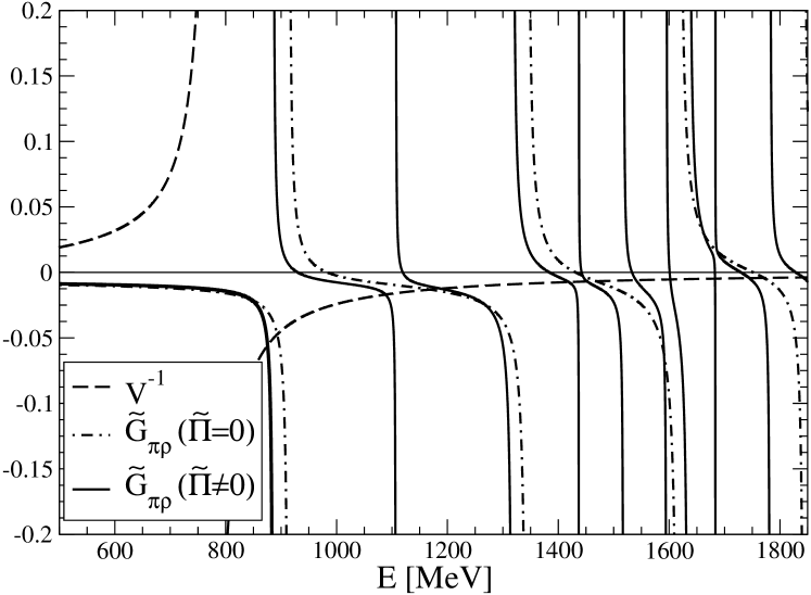
Figure 2: Loop function in the box $\widetilde{G}_{\pi\rho}$ (solid line) and $V^{-1}$ (dashed line) for $L=2m_{\pi}^{-1}$ and $p_{\textrm{max}}=1\textrm{ GeV}$. The dashed dotted line corresponds to the case with stable $\rho$, $\widetilde{\Pi}(s_{\rho})$=0.

In Fig. 2 we plot $V^{-1}$ and $\widetilde{G}_{\pi\rho}$ as a function of $E$ for $L=2m_{\pi}^{-1}$ and $p_{\textrm{max}}=1\textrm{ GeV}$. The $\widetilde{G}_{\pi\rho}$ plot is very different to a typical meson-meson loop function in infinite volume. It shows clear poles coming from zeros in the denominator of Eq. (31) and from poles of $\widetilde{\Pi}(s_{\rho})$. These poles of $\widetilde{G}_{\pi\rho}$ are not present in the infinite volume since in the integration the poles of the integrand provide an imaginary part to the loop function but not a pole after performing the integration. However, this is not the case in the finite box since we do not have an integral but a summation. The intersection between both plots of Fig. 2 just provides the $\pi\rho$ scattering eigenenergies in the box.

It is interesting to note that the spectra obtained is also qualitatively different to the one obtained for the stable $\rho$ which would be given by the intersection of $V^{-1}$ and $\widetilde{G}_{\pi\rho}$ for the case of the stable $\rho$ (dashed-dotted line in the figure). We can see that for stable $\rho$ one has $\widetilde{G}_{\pi\rho}$ going to infinity when the energy $E$ approaches one of the free energies of the $\pi\rho$ system in the box. Then $V^{-1}$ cuts $\widetilde{G}_{\pi\rho}$ only once in between two neighboring asymptotes. When we discretize the $\pi\pi$ system, $\widetilde{\Pi}(s_{\rho})$ becomes infinite for the discrete energies of the moving $\pi\pi$ system in the box. With $\widetilde{\Pi}(s_{\rho})$ becoming infinite, with plus and minus sign, in the denominator of Eq. (31), independently of the value of $E^{2}-(\omega_{1}+\omega_{2})^{2}$, close to the pole of $\widetilde{\Pi}(s_{\rho})$ there will be an energy where the denominator will vanish, leading to a pole of $\widetilde{G}_{\pi\rho}$. Thus, we get asymptotes of $\widetilde{G}_{\pi\rho}$ for values of E close to the free eigenenergies of $\pi\rho$ and also close to the free eigenenergies of the moving $\pi\pi$. We observe that in between two asymptotes corresponding to the $\pi\rho$ free eigenenergies (dashed dotted lines) one new asymptote has appeared corresponding to a free $\pi\pi$ eigenenergy of the $\pi\pi$ moving frame. As a result of it, the line $V^{-1}$ cuts now two lines corresponding to the unstable $\rho$ and only one corresponding to the stable $\rho$. If we go to higher energies we observe that in between the next two asymptotes corresponding to the free eigenenergies of $\pi\rho$ there are now three extra asymptotes corresponding to free eigenenergies of $\pi\pi$ in the moving frame. This leads now to four eigenenergies of the interacting $\pi\rho$ system in the box when we cut these lines with $V^{-1}$. There is, thus, a proliferation of eigenenergies as a consequence of considering the $\rho$ as an unstable state.

VII Results

VII.1 Energy levels in the box

We first show in Fig. 3 the solutions of Eq. (34) which represent the energy levels for different values of the cubic size, $L$. The solid lines represent the full calculation, considering the unstable $\rho$-meson via the consideration of its selfenergy in the box, $\widetilde{\Pi}$ in Eq. (31), and the dashed lines are the same calculation but setting $\widetilde{\Pi}=0$ in Eq. (31), i.e., considering the case of stable $\rho$ meson. There is an infinite number of levels and we have plotted the first six ones for illustration. This distribution of energy levels depends on the cutoff $p_{\textrm{max}}$ and in particular this figure has been evaluated using $p_{\textrm{max}}=1\textrm{ GeV}$ which is of the order of the cutoff used in Ref. luisaxial to get dynamically the axial-vector resonances.

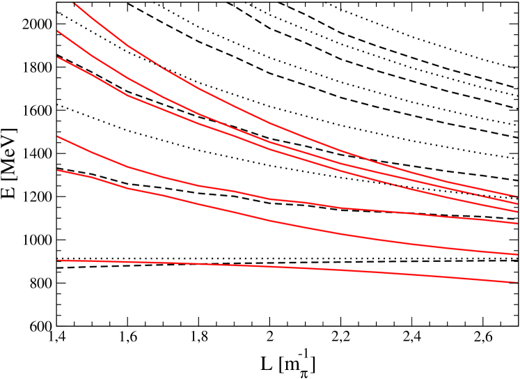
Figure 3: The first six energy levels as a function of the cubic box size $L$ for stable $\rho$-meson ($\widetilde{\Pi}=0$) (dashed lines) and for unstable $\rho$-meson (solid lines) using $p_{\textrm{max}}=1\textrm{ GeV}$. The dotted lines indicate the free $\pi\rho$ energies of the box for comparison.

It is worth noting the significant difference between the consideration of the unstable $\rho$ meson in comparison to the stable case. The main difference is that the levels tend to decrease and shrink as $L$ increases and that there are extra levels between those already present in the stable case, for instance between the second and third levels. This latter feature comes from the appearance of extra poles in $\widetilde{G}_{\pi\rho}$ due to the poles in $\widetilde{\Pi}$ and this produces extra intersections with the smooth function $V^{-1}$ as explained above. This different behavior between the stable and unstable analysis must be considered as a caveat for lattice calculations that only consider the stable case.

VII.2 Inverse problem: getting $\pi\rho$ amplitudes and phase shifts from lattice-like data

By “inverse problem” we refer to the problem of getting the actual scattering amplitudes (and hence by-product magnitudes like phase shifts) in the infinite space from data consisting of points over the energy levels in the box in the $E$ vs. $L$ plots, which is what a lattice calculation would provide. In our case we can “synthetically” simulate this lattice-like data from our model generating points in the levels of Fig. 3. We will call this data lattice-like set although in the present work it is generated from our model for illustrative purposes.

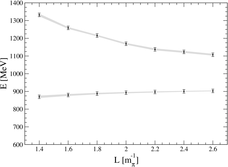
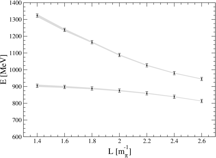
Figure 4: Synthesized lattice-like data considered in order to illustrate the inverse problem methods. Stable $\rho$ case: (a). Unstable $\rho$ case: (b). The error band represent the result of the fit in the fit method described in the text.

In Fig. 4 we represent by error bars the set generated for a particular election of $L$ values for the stable, 4, and unstable, 4, $\rho$ cases, to which we have assigned a reasonable error of $10\textrm{ MeV}$. The meaning of the shadowed error bands will be explained later in this section when explaining the fit method misha , hence they must be forgotten for the moment. We are aware that it is difficult for a present lattice calculation to get such quantity of points as considered in Fig. 4, but the method is equally valid for less points and we have chosen such a set just to illustrate more clearly the method. In an actual inverse problem the lattice-like generated set would just be replaced by actual lattice results.

In Refs. misha ; mishajuelich ; alberto ; mishakappa several methods were suggested to solve the inverse problem, mostly based on fitting the potential $V$ to reproduce lattice-like data analogous to those in Fig. 4. In the following we will call this method fit method. We will also discuss later the fit method for the present problem but first we want to propose a different strategy which does not require to assume a specific shape of the potential $V$, unlike the fit method. In the following we will call this new method direct method misha . The idea of the direct method is to evaluate directly the $\pi\rho$ amplitude using the expression

$$T_{\pi\rho}(E)=\frac{1}{\widetilde{G}_{\pi\rho}(E)-G_{\pi\rho}(E)}.$$ (35)

in the $p_{\textrm{max}}\to\infty$ limit with $G_{\pi\rho}(E)$ and $\widetilde{G}_{\pi\rho}(E)$ from Eqs. (30) and (31) for the energies of the points in Fig. 4. Recall that Eq. (35) is valid only for the energies solution of Eq. (34). Note that despite the fact that $G_{\pi\rho}(E)$ and $\widetilde{G}_{\pi\rho}(E)$ are divergent in the limit $p_{\textrm{max}}\to\infty$, the difference $\widetilde{G}_{\pi\rho}(E)-G_{\pi\rho}(E)$ which appears in Eq. (35) is convergent. Therefore Eq. (35) is cutoff independent. This is definitely a non-trivial result an illustrates one of the strong points of the method to solve the inverse problem. For practical numerical evaluations we have checked that considering an average in the interval $p_{\rm{max}}\sim[1.5,2.5]\textrm{ GeV}$ we get the same numerical result than considering $p_{\textrm{max}}\to\infty$. As shown in misha , Eq. (35) is a different and practical way of writing Lüscher’s equation, taking into account the full relativistic two body propagators.

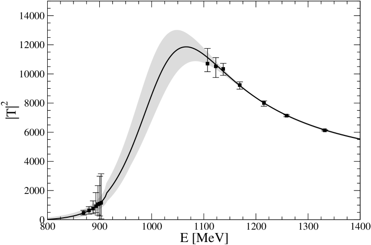
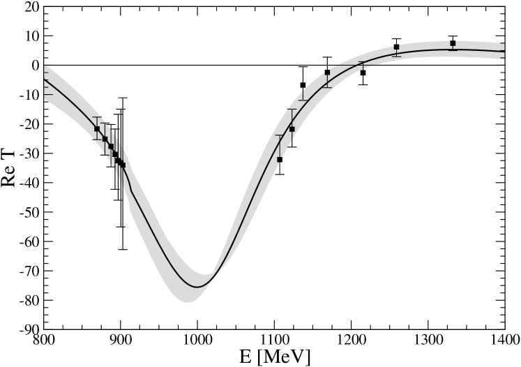
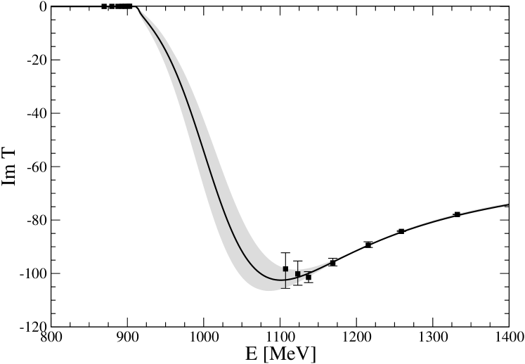
Figure 5: The $\pi\rho$ scattering amplitude solution of the inverse problem for the stable $\rho$ case. Horizontal errors of $\pm 10~{}MeV$ in the energy axis have to be also assumed. Square points with error bars: direct method. Solid line with error band: fit method

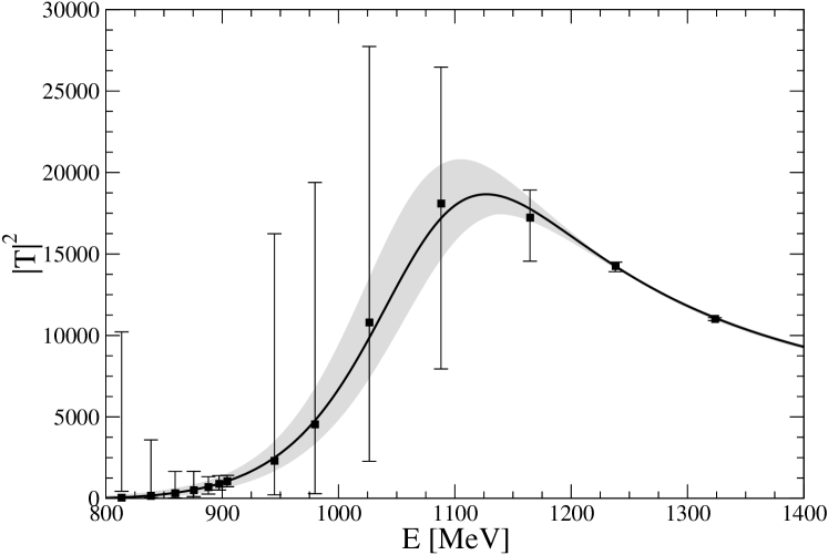
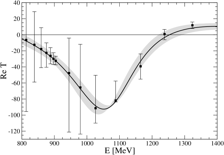
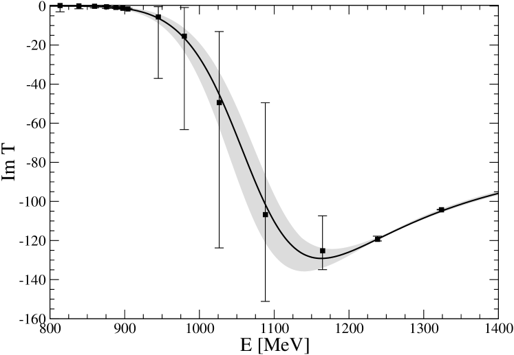
Figure 6: Same as Fig. 5 but for unstable $\rho$ meson

In Figs. 5 and 6 we represent by square points with error bars the $\pi\rho$ amplitude (modulus squared, real part and imaginary part) for the stable (Fig. 5) and unstable (Fig. 6) $\rho$ cases for the direct method. (The solid line and shadowed error bands represent the solution of the fit method which will be explained later on). The central points of the solution of the direct method are obtained with the central values of the lattice-like set and the error bars are evaluated by varying the energies within the $10\textrm{ MeV}$ errors given in Fig. 4. For the stable case there are no data points between 900 and 1100 MeV since, as can be seen in Fig. 3, one should go to very high values of the size of the box in order to get a good resolution in this energy region. It is worth noting that this method produces large errors for certain energies, particularly in the case of the unstable $\rho$. This is due to the fact that $\widetilde{G}_{\pi\rho}(E)$ is usually very steep close to the energy values of the levels (see Fig. 2) and, hence, small variations in $E$ provides large variations in $\widetilde{G}_{\pi\rho}(E)$. This feature can be seen in the $\widetilde{G}_{\pi\rho}$ vs. $E$ plot in Fig. 2 where it is visible that the crossing between the $V^{-1}$ and $\widetilde{G}_{\pi\rho}$ lines usually occur close to poles of $\widetilde{G}_{\pi\rho}$ and hence in an energy region where $\widetilde{G}_{\pi\rho}$ changes rapidly. Anyway, a clear resonance shape corresponding to the $a_{1}(1260)$ is visible as a peak in $|T|^{2}$. Note, however, that the shape is far from being a Breit-Wigner. The chiral unitary approach in which our lattice-like data set is generated, provides not only poles but the full scattering amplitude in the complex plane, in particular also in the real axis, and generates the possible background besides the pole, i.e., provides the actual shape of the amplitude. Actually, for the $a_{1}(1260)$ there is a very strong background which distorts the shape from a Breit-Wigner. The reason is that the amplitude is zero at around $E\simeq M_{\rho}$ since the potential $V$ is zero around that energy, as can be easily seen just looking for zeroes of Eq. (4) for the $\pi\rho$ case. However, the pole contribution itself has a large strength at this energy. This means that there must be a very strong background in order to cancel at that energy the tail of the Breit-Wigner shape coming from the pole in order to produce the zero. (See a more extended discussion on this zero in Ref. arXiv:0911.1235 ).

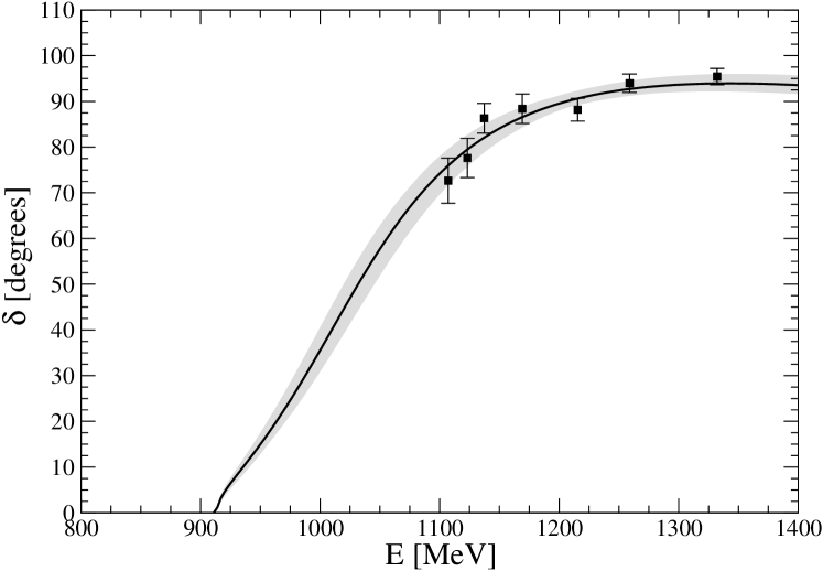
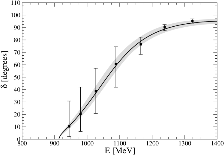
Figure 7: Phase shifts obtained from the solution of the inverse problem for the stable (a) and unstable (b) cases.Horizontal errors of $\pm 10~{}MeV$ in the energy axis have to be also assumed. Square points with error bars: direct method. Solid line with error band: fit method

From the scattering amplitudes we can get the phase shift, $\delta$, that is well defined for stable particle an which in our normalization it is related to the amplitude via

$$S=e^{2i\delta}=1-i\frac{p}{4\pi E}T{}$$ (36)

$$\Longrightarrow T(E)=-\frac{8\pi E}{p}\frac{1}{\cot\delta-i}.$$

where $p=\sqrt{(E^{2}-(m_{\rho}+m_{\pi})^{2})(E^{2}-(m_{\rho}-m_{\pi})^{2})}/(2E)$ is the CM momentum. Note that Eq. (36) is only well defined for stable scattering particles. However, for the sake of comparison between the stable and unstable case we also use, by definition for the unstable case, the same equation using for the $\rho$ meson mass the physical value, but being aware that in the unstable case this is not a well defined observable and it is just a theoretical mathematical exercise. The solutions of the inverse problem for the phase shifts using the direct method are shown by the squares and error bars in Fig. 7 for the stable, 7, and unstable, 7, cases. (Again the solid line and shadowed error bands represent the solution of the fit method explained below.)

It is interesting to note that the phase shifts that we have obtained are quite different from those of a Breit Wigner, where the phase shift would go from zero to 180 degrees passing through 90 degrees at the pole of the resonance. We see that the phase shifts stabilize around 90-100 degrees at high energies around 1400 MeV. On the other hand, the shape of $|T^{2}|$ in Fig. 5 is typical of a resonance, and bumps like that would be used to identify the resonance experimentally. To the light of this, and the comments above that the $\pi\rho$ amplitude has a strong background at low energies, one might question the procedure used in sashatalk where the shape of the amplitude is constructed from a calculated phase shift below threshold and another one above, assuming that one has a Breit Wigner amplitude. On the other hand, given the peculiar shape of the amplitude predicted here, the evaluation of phase shifts at physical energies in the energy range of our Fig. 7 would be most welcome. In this sense, it is interesting to note that the approach of sashatalk produces $\delta$ around 90 degrees in the region around 1430 MeV, where we find the phase shift stabilizing around that value (see Fig. 7).

Let us now apply the other method already introduced in Refs. misha ; alberto to solve the inverse problem based on fitting the potential, fit method.

The shape of the lowest order $\pi\rho$ potential, $V$, based on Eq. (4) which comes essentially from chiral symmetry, can be written in the form luisaxial :

$$V=a^{\prime}+b^{\prime}s+\frac{c^{\prime}}{s}.$$ (37)

In order to make the coefficients $a$, $b$ and $c$ adimensional and of natural order 1 we redefine the previous equation as

$$V\equiv\frac{-1}{4f_{\pi}^{2}}\left[m_{R}^{2}a+b(s-m_{R}^{2})-\frac{m_{\rho}^{2}}{s}c\right]$$ (38)

with $m_{R}=1.2\textrm{ GeV}$. Actually in Ref. luisaxial $a$, $b$ and $c$ were around 2, 1 and 3 respectively for the present channel, as can be obtained from Eq. (4). One should note that the expression of Eq. (38) is the one that one has in the chiral unitary approach. In this sense, the fit that we perform provides as a best solution the results of the chiral unitary approach with $\chi^{2}_{\rm{min}}=0$. One can give one self some freedom to have other possible potentials. When this is done what one finds is that the best solution is essentially the same but the uncertainties are somewhat larger mishakappa .

Next, we assume that lattice data are provided by our synthetic lattice-like set, points with error bars in Fig. 4. Then we fit these points with the solutions coming from Eq. (34) in order to get the best $a$, $b$ and $c$ parameters, which produce the minimum $\chi^{2}$, $\chi^{2}_{\rm{min}}$.

The $\widetilde{G}_{\pi\rho}(E)$ function is of course dependent on the cutoff $p_{\textrm{max}}$ and, therefore, also are the parameters fitted. However, the amplitude $T(E)$ obtained from Eq. (32) should be independent of this cutoff and therefore the inverse method does not require the knowledge or assumption of any particular cutoff, i.e., changing the cutoff value would produce different values for $a$, $b$ and $c$ but the amplitudes and observables derived from them would be the same. We have checked numerically that this is indeed the case within errors. This feature is not novel, it was already observed in misha and is related to the behavior of amplitudes within the renormalization group method, as used for instance in Quantum Mechanics in bengt .

In Fig. 4 we show with the solid line the result of the fit to the energy levels using for the fit the cutoff value $p_{\textrm{max}}=1\textrm{ GeV}$. The shadowed band represents the assigned errors obtained by varying the fitted parameters such that $\chi^{2}\leq\chi^{2}_{\rm{min}}+1$. From Fig. 5 till Fig. 7 we represent by the solid line and error bands the results of the fit method for the $\pi\rho$ amplitude and phase shift. Note that the fit method gives generally smaller errors than the direct method since it considers a global fit to all the points of the lattice-like set and does not suffer from the pathological error sensitivity discussed above for the direct method. However, it has the drawback of having to assume a shape of the potential, $V$, like in Eq. (37).

It is remarkable that in spite of the proliferation of eigenenergies in the case of the unstable $\rho$ and the different shapes of the two levels in Fig. 4 for the stable and unstable $\rho$, the amplitudes and the phase shifts in Figs. 5, 6 and 7 are rather similar. We observe then that the effects of considering the $\rho$ unstable are rather moderate in the previous analysis. This is not the case if we start from data generated with unstable $\rho$ but the inverse problem is analyzed with stable $\rho$, as will be explained at the end of this section. It is interesting to observe that the proliferation of levels in the case of the unstable $\rho$ has made the region of energies between threshold and 1400 MeV accessible, while for the stable $\rho$ the first accessible physical energies are around 1100 MeV. The price one pays for having these energies available in the unstable $\rho$ case is a bigger uncertainty in the reconstruction of the phase shifts as seen in Fig. 7.

Figure 8: The $\pi\rho$ scattering amplitude and phase shift solution of the inverse problem with the direct method with stable $\rho$ case but starting from data generated with unstable $\rho$.

At this point let us discuss a different analysis which may be closer to what a lattice calculation implements (see, however, some technical observations at the end of this section). In a real lattice calculation the generated data should be closer to those in Fig. 4, unstable $\rho$ case, since starting from quarks in the lattice and imposing on them the boundary conditions would naturally lead to boundary conditions in all the pions, the spectator and those coming from the $\rho$ decay. However, for simplicity, one may be tempted to do the subsequent analysis using the model for the stable $\rho$. In view of this, we are going to see what happens if one starts from a lattice-like set generated with the unstable model but the inverse problem is analyzed considering the stable case. Let us first focus on the direct method. Thus we evaluate now Eq. (35) for the case of stable $\rho$-meson but for the energies shown in Fig. 4. The results for the amplitude and phase shift are shown in Fig. 8. The result is very far from reality. The real part of the amplitude blows-up for low energies and it has little to do with the results of Figs. 5 or 6. The phase shift is also different to Fig. 7, even the sign. Conceptually there are no deep reasons why the results should be so different, but numerically the method is pathological for the following reasons. Let us focus on one energy where the extracted amplitude is very large, for instance the point of the lower energy band at $L=2.4\,m_{\pi}^{-1}$, for which $E=839\textrm{ MeV}$, (see Fig. 4). Let us look now at Fig. 9, where we show the same plots as in Fig. 2 but for $L=2.4\,m_{\pi}^{-1}$, (Fig. 2 was evaluated for $L=2\,m_{\pi}^{-1}$). The energy $E=839\textrm{ MeV}$ is indeed the first crossing point between $V^{-1}$ (dashed line) and $\widetilde{G}_{\pi\rho}(\widetilde{\Pi}\neq 0)$ (solid line). However, at this energy the value of $\widetilde{G}_{\pi\rho}(\widetilde{\Pi}=0)$ (dashed dotted line) is very different, about a factor six smaller. In Eq. (35), $G_{\pi\rho}$ is similar both for stable and unstable case and has a small value at this energy, (about -0.02). Therefore the amplitude evaluated with $\widetilde{G}_{\pi\rho}(\widetilde{\Pi}=0)$ is much larger than the one evaluated with $\widetilde{G}_{\pi\rho}(\widetilde{\Pi}\neq 0)$. On the other hand, the extra poles in $\widetilde{G}_{\pi\rho}(\widetilde{\Pi}\neq 0)$ coming from the eigenenergies of the $\pi\pi$ system as explained above, make the plot of $\widetilde{G}_{\pi\rho}(\widetilde{\Pi}\neq 0)$ very different from $\widetilde{G}_{\pi\rho}(\widetilde{\Pi}=0)$. Thus, close to an extra pole this numerical analysis is also inappropriate, since one would be misidentifying the poles responsible for the eigenvalues using the two procedures. These pathological behaviors of the $G_{\pi\rho}$ functions within the box are essentially due to the abruptness produced by the poles of the $G$ function in the box and it makes very difficult to extract reliable information from this analysis. We have also implemented the fit method in the last analysis, with stable $\rho$ but starting from data created with unstable $\rho$. In this case, no good fit is obtained since with this shape of the potential it is not possible to generate a curve decreasing with $L$ as the lower level in Fig. 4 does. Actually the best fit has a $\chi^{2}\sim 200$ and produces the pole for the $a_{1}$ in the real axis below threshold which makes also this analysis unreliable. The main conclusion of the analysis using the stable case but starting from data generated using unstable $\rho$ meson is that the inverse method should be as close as possible to reality, which in this context means to consider the unstable $\rho$ meson in the analysis of the data. Otherwise unreliable results could be obtained due to the abrupt shape of the $G$ functions in the box.

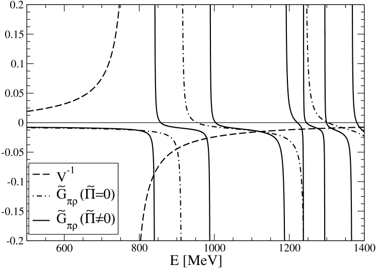
Figure 9: Same as Fig. 2 but for $L=2.4\,m_{\pi}^{-1}$.

In practice, the above mentioned problem could not show up in some actual lattice calculations, like in sashatalk , if large pion masses are used. Indeed, we have seen that with the pion mass $m_{\pi}=266MeV$, used in sashatalk , the ground state level is much less affected than in the case shown here, and the extra level originating from $\widetilde{\Pi}\neq 0$, which in Fig. 9 corresponds to the first excited state (eigenenergy around 1 GeV in the figure), is moved beyond the level corresponding to the first excited $\rho\pi$ state. In this case the results with the analysis with stable $\rho$ would be similar to those with the unstable $\rho$. Furthermore, one should also take into account that actual simulations like the one of sashatalk , which do not incorporate three-pion correlators, would not see the decay of the $\rho$ into $\pi\pi$, in which case, the analysis with a stable $\rho$ would be more appropriate to interprete such lattice results.

VIII Summary

We showed how to tackle the problem of the interaction of two particles quantized in a finite box of size $L$ when one of the them has a finite width. The idea is based on extending previously known techniques for the stable case but quantizing also inside this finite box the decay channel of the unstable particle. In this way, the continuous integration needed to evaluate the selfenergy is substituted by a discrete sum over the allowed levels in the box of the decay channel of the unstable scattering particle. We illustrate the method with the $\pi\rho$ scattering which generates dynamically the $a_{1}(1260)$ resonance within the chiral unitary approach. The scattering energy levels inside the box for periodic boundary conditions, both for the stable and unstable case are compared. The results show significant differences between both cases.

Then we explain how to solve the inverse problem of getting physical observables in the real world (infinite volume) from lattice data which are computed in a finite box. The idea is based on the improvement of the Lüscher’s approach developed in Ref. misha , properly adapted to the present problem. We apply two methods to solve the inverse problem: the first one is a previously proposed way based on fitting the parameters of a given potential to get the lattice data energy levels, fit method. The second one, direct method, is to evaluate directly the $\pi\rho$ amplitude using Eq. (35). The advantage of the direct method, which is closer to the original Lüscher approach, is that there is no need to provide a specific shape of the potential since there is no potential involved. However, the drawback is that the errors are larger than in the fit method and that the observables in the infinite volume can be evaluated only for those energies for which there are lattice data.

With respect to the particular case studied here of the $\pi\rho$ scattering and the $a_{1}$ resonance, it is quite instructive to observe that the amplitudes obtained are rather peculiar and they do not resemble much the shape of a Breit Wigner. This feature will have to be considered in future lattice QCD studies. We showed that using the stable $\rho$, the first physical energies accessible were around 1100 MeV. However, the proliferation of energy levels due to the quantization of the decay products of the $\rho$, making the study with the unstable $\rho$, made a wider range of energies available, although the induced phase shifts had larger errors using the direct Lüscher method. In such a case, the $fit~{}method$ proposed here could provide a more efficient method to induce the phase shifts with much smaller errors.

Furthermore, we have also discussed that if the starting generated lattice data takes into account the decay of the $\rho$ meson into two pions, then the analysis of the inverse problem must be performed considering also the instability of the $\rho$ meson. Otherwise the results could be numerically unreliable.

The considerations done in the present work should spur the future lattice calculations to consider also the discretization of the decay channels when unstable particles are involved in the scattering. In between, calculations along the line of sashatalk , which can be studied with the stable $\rho$ analysis, produced at other volumes or within a moving frame, could bring extra information on phase shifts in the physical region which would eventually determine the peculiar shape of $\pi\rho$ amplitude in the $a_{1}$ resonance region, with a strong diversion from a Breit Wigner shape.

References

- (1) Y. Nakahara, M. Asakawa, T. Hatsuda, Phys. Rev. D60 (1999) 091503. K. Sasaki, S. Sasaki and T. Hatsuda, Phys. Lett. B 623 (2005) 208.
- (2) N. Mathur, A. Alexandru, Y. Chen et al., Phys. Rev. D76 (2007) 114505.
- (3) S. Basak, R. G. Edwards, G. T. Fleming et al., Phys. Rev. D76 (2007) 074504.
- (4) J. Bulava, R. G. Edwards, E. Engelson et al., Phys. Rev. D82 (2010) 014507.
- (5) C. Morningstar, A. Bell, J. Bulava et al., AIP Conf. Proc. 1257 (2010) 779.
- (6) J. Foley, J. Bulava, K. J. Juge et al., AIP Conf. Proc. 1257 (2010) 789.
- (7) M. G. Alford and R. L. Jaffe, Nucl. Phys. B 578 (2000) 367.
- (8) T. Kunihiro, S. Muroya, A. Nakamura, C. Nonaka, M. Sekiguchi and H. Wada [SCALAR Collaboration], Phys. Rev. D 70 (2004) 034504.
- (9) F. Okiharu et al., arXiv:hep-ph/0507187. H. Suganuma, K. Tsumura, N. Ishii and F. Okiharu, PoS LAT2005 (2006) 070; Prog. Theor. Phys. Suppl. 168 (2007) 168.
- (10) C. McNeile and C. Michael [UKQCD Collaboration], Phys. Rev. D 74 (2006) 014508. A. Hart, C. McNeile, C. Michael and J. Pickavance [UKQCD Collaboration], Phys. Rev. D 74 (2006) 114504.
- (11) H. Wada, T. Kunihiro, S. Muroya, A. Nakamura, C. Nonaka and M. Sekiguchi, Phys. Lett. B 652 (2007) 250.
- (12) S. Prelovsek, C. Dawson, T. Izubuchi, K. Orginos and A. Soni, Phys. Rev. D 70 (2004) 094503. S. Prelovsek, T. Draper, C. B. Lang, M. Limmer, K. F. Liu, N. Mathur and D. Mohler, Conf. Proc. C 0908171 (2009) 508; Phys. Rev. D 82 (2010) 094507
- (13) H. -W. Lin et al. [ Hadron Spectrum Collaboration ], Phys. Rev. D79, 034502 (2009).
- (14) C. Gattringer, C. Hagen, C. B. Lang, M. Limmer, D. Mohler, A. Schafer, Phys. Rev. D79, 054501 (2009).
- (15) G. P. Engel et al. [ BGR [Bern-Graz-Regensburg] Collaboration ], Phys. Rev. D82, 034505 (2010).
- (16) M. S. Mahbub, W. Kamleh, D. B. Leinweber, A. O Cais, A. G. Williams, Phys. Lett. B693, 351-357 (2010).
- (17) R. G. Edwards, J. J. Dudek, D. G. Richards, S. J. Wallace, Phys. Rev. D84, 074508 (2011).
- (18) V. Bernard, U. -G. Meissner, A. Rusetsky, Nucl. Phys. B788, 1-20 (2008).
- (19) V. Bernard, M. Lage, U. -G. Meissner, A. Rusetsky, JHEP 0808, 024 (2008).
- (20) M. Doring, U. -G. Meissner, E. Oset and A. Rusetsky, Eur. Phys. J. A 47, 139 (2011).
- (21) M. Lüscher, Commun. Math. Phys. 105 (1986) 153 (1986).
- (22) M. Lüscher, Nucl. Phys. B 354 (1991) 531.
- (23) M. Doring, J. Haidenbauer, U. -G. Meissner, A. Rusetsky, [arXiv:1108.0676 [hep-lat]]. Eur. Phys. J. A, in print.
- (24) A. M. Torres, L. R. Dai, C. Koren, D. Jido, E. Oset, [arXiv:1109.0396 [hep-lat]].
- (25) E. E. Kolomeitsev, M. F. M. Lutz, Phys. Lett. B582, 39-48 (2004).
- (26) J. Hofmann, M. F. M. Lutz, Nucl. Phys. A733, 142-152 (2004).
- (27) F. -K. Guo, P. -N. Shen, H. -C. Chiang, R. -G. Ping, B. -S. Zou, Phys. Lett. B641, 278-285 (2006).
- (28) D. Gamermann, E. Oset, D. Strottman, M. J. Vicente Vacas, Phys. Rev. D76, 074016 (2007).
- (29) M. Doring, U. G. Meissner, [arXiv:1111.0616 [hep-lat]].
- (30) M. Doring et al, to be submitted.
- (31) S. Prelovsek, C. B. Lang, D. Mohler and M. Vidmar, [arXiv:1111.0409 [hep-lat]].
- (32) M. F. M. Lutz, E. E. Kolomeitsev, Nucl. Phys. A730, 392-416 (2004).
- (33) L. Roca, E. Oset, J. Singh, Phys. Rev. D72, 014002 (2005).
- (34) K. Rummukainen, S. A. Gottlieb, Nucl. Phys. B450, 397-436 (1995).
- (35) C. h. Kim, C. T. Sachrajda, S. R. Sharpe, Nucl. Phys. B727, 218-243 (2005).
- (36) M. C. Birse, Z. Phys. A 355 (1996) 231.
- (37) J. A. Oller, U. G. Meissner, Phys. Lett. B500, 263-272 (2001).
- (38) J. A. Oller, E. Oset and J. R. Pelaez, Phys. Rev. D 59 (1999) 074001 [Erratum-ibid. D 60 (1999) 099906] [Erratum-ibid. D 75 (2007) 099903].
- (39) E. Oset, A. Ramos, C. Bennhold, Phys. Lett. B527, 99-105 (2002).
- (40) J. A. Oller, E. Oset, Nucl. Phys. A620, 438-456 (1997).
- (41) M. Bando, T. Kugo, S. Uehara, K. Yamawaki and T. Yanagida, Phys. Rev. Lett. 54 (1985) 1215; M. Bando, T. Kugo and K. Yamawaki, Phys. Rept. 164 (1988) 217; M. Harada and K. Yamawaki, Phys. Rept. 381, 1 (2003).
- (42) J. A. Oller, E. Oset and J. E. Palomar, Phys. Rev. D 63 (2001) 114009.
- (43) P. Fernandez de Cordoba, Y. .Ratis, E. Oset, J. Nieves, M. J. Vicente-Vacas, B. Lopez-Alvaredo and F. Gareev, Nucl. Phys. A 586 (1995) 586.
- (44) D. Cabrera, D. Jido, R. Rapp and L. Roca, Prog. Theor. Phys. 123 (2010) 719.
- (45) A. Schwenk, B. Friman and G. E. Brown, Nucl. Phys. A 713, 191 (2003).