The $DN$, $\pi\Sigma_{c}$ interaction in finite volume and the $\Lambda_{c}(2595)$ resonance

Abstract

In this work the interaction of the coupled channels $DN$ and $\pi\Sigma_{c}$ in an SU(4) extrapolation of the chiral unitary theory, where the $\Lambda_{c}(2595)$ resonance appears as dynamically generated from that interaction, is extended to produce results in finite volume. Energy levels in the finite box are evaluated and, assuming that they would correspond to lattice results, the inverse problem of determining the phase shifts in the infinite volume from the lattice results is solved. We observe that it is possible to obtain accurate $\pi\Sigma_{c}$ phase shifts and the position of the $\Lambda_{c}(2595)$ resonance, but it requires the explicit consideration of the two coupled channels. We also observe that some of the energy levels in the box are attached to the closed $DN$ channel, such that their use to induce the $\pi\Sigma_{c}$ phase shifts via Lüscher’s formula leads to incorrect results.

I Introduction

One of the topics where efforts are recently devoted within Lattice QCD is the determination of hadron spectra, both in the meson and baryon sector Nakahara:1999vy1 ; Nakahara:1999vy2 ; Mathur:2006bs ; Basak:2007kj ; Bulava:2010yg ; Morningstar:2010ae ; Foley:2010te ; Alford:2000mm ; Kunihiro:2003yj ; Suganuma:2005ds1 ; Suganuma:2005ds2 ; Hart:2006ps1 ; Hart:2006ps2 ; Wada:2007cp ; Prelovsek:2010gm1 ; Prelovsek:2010gm2 ; Lin:2008pr ; Gattringer:2008vj ; Engel:2010my ; Mahbub:2010me ; Edwards:2011jj . After earlier claims of a successful determination of the hadron spectra using rough approximations and large pion masses, work continues along this line with more accurate approaches and problems are arising that were not envisaged at first glance. The ”avoided level crossing” is usually taken as a signal of a resonance, but this criteria has been shown insufficient for resonances with a large width Bernard:2007cm ; Bernard:2008ax ; misha . The use of Lüscher’s approach luscher ; Luscher:1990ux is gradually catching up. It is suited for the case when one has resonances with one decay channel in order to produce phase shifts for this decay channel from the discrete energy levels in the box. Yet, most of the hadronic resonances have two or more decay channels and the need to go beyond Lüscher’s approach becomes obvious. This method has been recently improved in Ref. misha by keeping the full relativistic two body propagator (Lüscher’s approach has an exact imaginary part but makes approximations on the real part) and extending the method to two, or more coupled channels, which had also been addressed before Liu:2005kr ; Lage:2009zv ; Bernard:2010fp , and continues to catch the attention of the practitioners sharpe ; davoudi . The new method is also conceptually and technically simpler and serves as a guideline for future lattice calculations. Continuation of this new practical method have been done in Ref. mishajuelich for the application of the Jülich approach to meson baryon interaction and in Ref. alberto for the interaction of the $DK$ and $\eta D_{s}$ system where the $D_{s^{*}0}(2317)$ resonance is dynamically generated from the interaction of these particles Kolomeitsev:2003ac ; Hofmann:2003je ; Guo:2006fu ; daniel . The case of the $\kappa$ resonance in the $K\pi$ channel is also addressed along the lines of Ref. misha in Ref. mishakappa .

The investigation of different problems following Refs. misha ; mishajuelich ; alberto ; mishakappa is showing that every case studied reveals particular features and there is no common behaviour in the levels of the finite box nor on the way that the phase shifts or bound states are obtained from the spectra of the finite box. The study of these problems along those lines is most useful, since it sheds light on how to deal with results of QCD lattice calculations, which precision is needed in the lattice results to accomplish a desired accuracy in the phase shifts or resonance pole positions, and which strategy is most useful to gather lattice results from where the results in infinite volume can be obtained with maximum accuracy.

The case we report here is one more in this line, showing as a novel feature how in this case some of the low lying levels in the finite box, for energies where the $\pi\Sigma_{c}$ channel is open and the $DN$ one is closed, are tied basically to the $DN$ channel, such that the blind use of Lüscher’s approach would lead to unrealistic phase shifts for the $\pi\Sigma_{c}$ channel and the resonance position. We show the problems that arise in this analysis and provide the two channel approach to solve them. These results should be most useful when QCD lattice results are produced to describe the $\Lambda_{c}(2595)$ resonance.

This paper is organized as follows. In Sec. II we show the formalism of the $DN$ and $\pi\Sigma_{c}$ interaction in infinite and finite volume. In Sec. III, the inverse problem of getting the phase shifts from two channels analysis is shown, while in Sec. IV the results obtained by using one channel analysis are shown. Finally, a short summary is given in Sec. V.

II Formalism

II.1 The $DN$, $\pi\Sigma_{c}$ interaction in infinite volume

The $DN$ system, in collaboration with coupled channels, leads to the formation of a meson-baryon composite state, the $\Lambda_{c}(2595)$ hofmannnpa763 ; mizutaniprc74 ; tolosprc77 ; juanprd79 . In this section, we briefly revisit the form of the $\pi\Sigma_{c}$ and $DN$ interactions from the chiral unitary approach. This will allow us to review the general procedure of calculating meson-baryon scattering amplitudes. In the chiral unitary approach the scattering matrix in coupled channels is given by

$$T=[1-VG]^{-1}V$$ (1)

where $V$ is the matrix for the transition potentials between the channels and $G$, a diagonal matrix, is the loop function for intermediate $\pi\Sigma_{c}$ and $DN$ states, which is defined as

$$G=i\int\frac{d^{4}q}{(2\pi)^{4}}\frac{1}{q^{2}-m^{2}+i\epsilon}\frac{2M}{(P-q)^{2}-M^{2}+i\epsilon}\,$$ (2)

where $m$ and $M$ are the masses of the $\pi$ or $D$ meson and the baryon $\Sigma_{c}$ or $N$, respectively. In the above equation, $P$ is the total incident momentum of the external meson-baryon system.

In the present problem we have two main channels, $\pi\Sigma_{c}$ and $DN$. There are also other channels considered in Refs. mizutaniprc74 ; tolosprc77 ; juanprd79 , such as $\eta\Lambda_{c}$, $K\Xi_{c}$, $K\Xi_{c}^{\prime}$, $D_{s}\Lambda$, and $\eta^{\prime}\Lambda_{c}$, which play a negligible role to generate dynamically the $\Lambda_{c}(2595)$ state, and are not considered here.

We study only the $s$-wave interaction, hence, the transition interaction (potential) for channel $i$ to $j$ reads,

$$V_{ij} = -\frac{C_{ij}}{4f^{2}}(2\sqrt{s}-M_{i}-M_{j})$$ (3)

$$\times\left(\frac{M_{i}+E_{i}}{2M_{i}}\right)^{1/2}\left(\frac{M_{j}+E_{j}}{2M_{j}}\right)^{1/2},$$

where $f=93$ MeV is the pion decay constant, $E_{i}$ and $E_{j}$ are the energy of incoming/outgoing baryon $\Sigma_{c}$ or $N$. The transition coefficients $C_{ij}$ are symmetric with respect to the indices, and also isospin-dependent. By naming the channels, 1 for $\pi\Sigma_{c}$ and 2 for $DN$, the coefficients $C_{ij}$ for the case of isospin $I=0$ are mizutaniprc74

$$C_{11}=4,\hskip 14.22636ptC_{12}=C_{21}=\frac{\sqrt{6}}{8},\hskip 14.22636ptC_{22}=3.$$ (4)

The loop function $G$ can be regularized both with a cutoff prescription or with dimensional regularization in terms of a subtraction constant. Here we make use of the dimensional regularization scheme. The expression for $G$ is then

$$\mbox{G}^{D}_{i}(s,m_{i},M_{i}) = \frac{2M_{i}}{(4\pi)^{2}}\left\{a_{i}(\mu)+\log\frac{m_{i}^{2}}{\mu^{2}}+\frac{M_{i}^{2}-m_{i}^{2}+s}{2s}\log\frac{M_{i}^{2}}{m_{i}^{2}}\right.$$

$$+ \frac{Q_{i}(\sqrt{s})}{\sqrt{s}}\left[\log\left(s-(M_{i}^{2}-m_{i}^{2})+2\sqrt{s}Q_{i}(\sqrt{s})\right)+\log\left(s+(M_{i}^{2}-m_{i}^{2})+2\sqrt{s}Q_{i}(\sqrt{s})\right)\right.$$

$$- \Biggl{.}\left.\log\left(-s+(M_{i}^{2}-m_{i}^{2})+2\sqrt{s}Q_{i}(\sqrt{s})\right)-\log\left(-s-(M_{i}^{2}-m_{i}^{2})+2\sqrt{s}Q_{i}(\sqrt{s})\right)\right]\Biggr{\}},$$

where $s=E^{2}$, with $E$ the energy of the system in the center of mass frame, $Q_{i}$ the on shell momentum of the particles in the channel, $\mu$ a regularization scale and $a_{i}(\mu)$ a subtraction constant. The form of Eq. (3) is adapted from the light hadron sector to the charm sector using SU(4) symmetry but reducing the strength of the diagrams with a heavy vector exchange by the weight of its propagator. One should, in principle, not expect a good SU(4) symmetry, and actually it is broken in this case through the use of physical masses in the propagator. But in basic vertices the symmetry works quite well (see an extensive review in Ref. danithesis and references therein, and in section IV of the paper wu ). We thus follow this approach, as done in Refs. hofmannnpa763 ; mizutaniprc74 ; tolosprc77 ; juanprd79 . One must bear in mind that uncertainties in the actual value of $V_{ij}$ in Eq. (3) are taken into account, in the spirit of the renormalization group, by means of the freedom in the subtraction constants of $G$ in Eq. (II.1), which are adjusted such as to get the energy of the $\Lambda_{c}(2595)$ in the right place. Note that the only parameter-dependent part of $G$ is $a(\mu)+\text{ln}\frac{m^{2}_{i}}{\mu^{2}}$. Any change in $\mu$ is reabsorbed by a change in $a(\mu)$ through $a(\mu^{\prime})-a(\mu)=\text{ln}\frac{\mu^{\prime 2}}{\mu^{2}}$.

In the infinite volume case, the use of Eq. (1) with the two channels that we consider leads to a dynamically generated state at the energy of $2596$ MeV, which we associate to the $\Lambda_{c}(2595)$ resonance, using the dimensionally regularized $G^{D}$ function with $\mu=1000$ MeV and the subtraction constant $a=-2.02$, which are values of natural size. In Fig. 1 the modulus squared of the $DN\to DN$ scattering amplitude as a function of the invariant mass of the $DN$ system for $I_{DN}=0$ is shown. There is a clear rather narrow peak around $2596$ MeV which indicates the state of $\Lambda_{c}(2595)$ as a bound state of $DN$.

Figure 1: Modulus squared of the $DN\to DN$ scattering amplitude for $I_{DN}=0$.

The poles of the amplitudes are found in the second Riemann sheet, where in the loop function $G^{D}$ in Eq. (II.1) $Q_{i}(\sqrt{s})$ is changed to $-Q_{i}(\sqrt{s})$ for the channel where ${\rm Re}\sqrt{s}$ is above threshold. The couplings of $\Lambda_{c}(2595)$ to the $\pi\Sigma_{c}$ and $DN$ channels can be obtained from the residues at the pole, by matching the amplitudes to the expression

$$T_{ij}=\frac{g_{i}g_{j}}{\sqrt{s}-\sqrt{s_{R}}}$$ (6)

for $\sqrt{s}$ close to the pole $\sqrt{s_{R}}$. We find $\sqrt{s_{R}}=(2596.3-i1.6)$ MeV. The couplings, $g_{i}$ and $g_{j}$ are complex in general. In this way, we get $g^{2}_{\pi\Sigma_{c}}=0.65-i0.10$ and $g^{2}_{DN}=43.3+i3.6$.

In Ref. arriola , an analytical study of bound states in problems with coupled channels has been performed. A modern formulation of the compositeness condition of Weinberg weinberg for coupled channels has been derived from a sum rule that comes from the normalization to unity of the wave function of the bound state ,

$$\sum_{i}g_{i}^{2}\left.\frac{dG_{ii}}{dE}\right|_{E=E_{\alpha}}=-1,$$ (7)

where $g_{i}^{2}$ are the residues of the $T_{ii}$ scattering matrices (coupling squared) at the pole of the bound state ($\alpha$) and $G_{ii}$ are the propagators of the two particles of the corresponding channels (the loop function $G^{D}$ that we use here).

One can see from the derivation in Ref. arriola that each term in Eq. (7) accounts (with reversed sign) for the probability of the bound state to be made by the pair of particles of the channel considered. By taking the coupling constant $g^{2}_{DN}$ that we obtained above and the loop function $G^{D}_{DN}$, we find that $g^{2}_{DN}\frac{dG^{D}_{DN}}{dE}=-0.91-i0.08$ at $E=\sqrt{s_{R}}$, and, thus, about $91\%$ of the sum rule comes from the $DN$ state, indicating that we have largely a bound $DN$ channel in our approach.

Another way to check how important is the $DN$ channel in generating dynamically of the $\Lambda_{c}(2595)$ state is to change the parameters of the potential slightly, making the $\Lambda_{c}(2595)$ disappear. This can be achieved, for example, by merely reducing the strength of the potential $V_{22}$ that describes the scattering in the $DN\to DN$ channel. Namely, we replace $V_{22}\to\eta V_{22}$ and vary $\eta$ between 1 and 0, and as can be seen in Fig. 2, the phase shifts for the $\pi\Sigma_{c}\to\pi\Sigma_{c}$ scattering amplitude obtained from the Bethe-Salpeter equation, Eq. (1), drastically change with the strength of $V_{22}$. The normalization that we use is such that in one channel ollernpa620  

$$T(E)=\frac{1}{2m_{\Sigma_{c}}}\frac{-8\pi E}{p\cot\delta(p)-i\,p}\,,$$ (8)

from where we determine the phase shifts in the infinite volume problem.

Figure 2: Phase shift for $\pi\Sigma_{c}$ scattering derived from the coupled channels unitary approach with different values of $\eta$. Solid line: $\eta=1$. Dashed line: $\eta=0.8$. Dotted line: only $\pi\Sigma_{c}$ channel considered.

In Fig. 2, the solid curve stands for the phase shifts for $\pi\Sigma_{c}$ scattering derived from the two coupled channels unitary approach with $\eta=1$, while the dashed line is obtained with $\eta=0.8$. We also show with the dotted line the phase shifts that were obtained considering only the $\pi\Sigma_{c}$ channel.

II.2 The $DN$, $\pi\Sigma_{c}$ interaction in finite volume

One can also use regularization with a cut off in three momentum once the $q^{0}$ integration is analytically performed ollernpa620 with the result

$$G_{j} = \int\limits^{|\vec{q}|<q_{\rm max}}\frac{d^{3}\vec{q}}{(2\pi)^{3}}\frac{2m_{2}}{2\omega_{1}(\vec{q})\,\omega_{2}(\vec{q})}$$

$$\times\frac{\omega_{1}(\vec{q})+\omega_{2}(\vec{q})}{E^{2}-(\omega_{1}(\vec{q})+\omega_{2}(\vec{q}))^{2}+i\epsilon},$$

$$\omega_{1,2}(\vec{q}) = \sqrt{m_{1,2}^{2}+\vec{q}^{\,\,2}}\,,$$ (9)

with $m_{1}$, $m_{2}$ corresponding to $m$ and $M$ of Eq. (2) for each channel $j$. In Ref. ollerulf the equivalence of the two methods was established.

When one wants to obtain the energy levels in the box, one replaces the $G$ function by $\tilde{G}$, where instead of integrating over the energy states of the infinite volume, with $q=|\,\vec{q}\,|$ being a continuous variable, as in Eq. (9), one sums over the discrete momenta allowed in a finite box of side $L$ with periodic boundary conditions. We then have $\tilde{G}={\rm diag}\,(\tilde{G}_{1},\tilde{G}_{2})$, where

$$\tilde{G}_{j} = \frac{1}{L^{3}}\sum_{\vec{q}}^{|\vec{q}|<q_{\rm max}}\frac{2m_{2}}{2\omega_{1}(\vec{q})\,\omega_{2}(\vec{q})}\,\,\frac{\omega_{1}(\vec{q})+\omega_{2}(\vec{q})}{E^{2}-(\omega_{1}(\vec{q})+\omega_{2}(\vec{q}))^{2}},$$

$$\vec{q} = \frac{2\pi}{L}\,\vec{n},\quad\vec{n}\in{Z}^{3},$$ (10)

with the same notation as in Eq. (9).

By using the dimensional regularization of the loop function $G^{D}$ of Eq. (II.1), we can write alberto

$$\tilde{G}(E) =G^{D}(E)$$

$$+\lim_{q_{\rm max}\to\infty}\Bigg{[}\frac{1}{L^{3}}\sum_{\vec{q}}^{|\vec{q}|<q_{\rm max}}I(\vec{q})-\int\limits_{q<q_{\rm max}}\frac{d^{3}q}{(2\pi)^{3}}I(\vec{q})\Bigg{]}$$

$$\equiv G^{D}(E)+B,$$ (11)

where $I(\vec{q})$ is the integrand of Eq. (9)

$$I(\vec{q}) = \frac{2m_{2}}{2\omega_{1}(\vec{q})\,\omega_{2}(\vec{q})}\frac{\omega_{1}(\vec{q})+\omega_{2}(\vec{q})}{E^{2}-(\omega_{1}(\vec{q})+\omega_{2}(\vec{q}))^{2}+i\epsilon}.$$ (12)

The three dimensional sum in Eq. (11) can be reduced to one dimension considering the multiplicities of the cases having the same $\vec{n}^{\,2}$  mishajuelich ; c . The integral in Eq. (11) has an analytical form as shown in the appendix of Ref. d (see erratum).

In the box, the same Bethe-Salpeter equation is used substituting $G^{D}$ by $\tilde{G}$ of Eq. (11). When calculating the limit of $q_{max}$ going to infinity in Eq. (11) we obtain oscillations which gradually vanish as $q_{max}$ goes to infinity. Yet it is unnecessary to go to large values of $q_{max}$, and performing an average for different $q_{max}$ values between $2000$ MeV and $4000$ MeV one obtains a perfect convergence, as one can see in Fig. 3. Note that the imaginary part of $G^{D}$ and that of the integral in Eq. (11) are identical and they cancel in the construction of $\tilde{G}$, which is a real function.

Figure 3: Real part of the second part of Eq. (11) for the $\pi\Sigma_{c}$ channel. The dashed line stands for the average that we take between $2000$ MeV and $4000$ MeV for $q_{max}$. The results correspond to a value of $L=2.5~{}m_{\pi}^{-1}$ and E$=2600$ MeV.

The eigenenergies of the box correspond to energies that produce poles in the $T$ matrix. Thus we search for these energies by looking for zeros of the determinant of $1-V\tilde{G}$

$$\det(1-V\tilde{G}) = 1-V_{11}\tilde{G}_{1}-V_{22}\tilde{G}_{2}$$ (13)

$$+(V_{11}V_{22}-V_{12}^{2})\tilde{G}_{1}\tilde{G}_{2}=0\,.$$

In Fig. 4 we show the first five energy levels obtained for the box for different values of $L$. We observe a smooth behavior of the levels as a function of $L$. The second level is special because it mainly comes from the $DN$ channel. If we only include the $DN$ channel, we get very similar results as shown with the dashed curve. From Fig. 4 we can also see that the second level is rather independent on the values of the cubic box size $L$. The value for the eigenenergy of the second level is around $2600$ MeV which is very close to the mass of $\Lambda_{c}(2595)$.

Figure 4: Energy levels as functions of the cubic box size $L(m^{-1}_{\pi})$, derived from the chiral unitary approach.

III The inverse problem of getting phase shifts from lattice data

In this section we face the problem of getting bound states and phase shifts in the infinite volume from the energy levels obtained in the box using the two channel approach of Ref. mizutaniprc74 , which we would consider as “synthetic” lattice data. To accomplish this we need more information than just the lowest level, but we shall see that the first two levels shown in Fig. 4 already provide the necessary information to reproduce the problem in the infinite volume.

In Ref. misha several methods were suggested to solve the inverse problem, one of the methods was the following: In two channels one has three degrees of freedom, $V_{11}$, $V_{12}$, and $V_{22}$, or in terms of phase shifts, $\delta_{1}$, $\delta_{2}$ and the inelasticity $\eta$ (or equivalently the mixing angle). One strategy to obtain these magnitudes is to use three levels that contain a certain energy and using Eq. (13) determine the three degrees of freedom for a given energy. This strategy is used in [20] and is also suggested in sharpe ; davoudi to obtain directly $\delta_{1}$, $\delta_{2}$ and $\eta$. The technical problem that this method poses is that for a given energy one might need a too large or a too small value of $L$ that could make the computation too lengthy or inaccurate, respectively, although using moving frames, like in sharpe ; davoudi one obtains more levels that can reduce the span of values of $L$. Other different methods were suggested in Ref. misha and we borrow here the one based on a fit to the data in terms of a potential parameterized as a function of the energy suggested by the coupled channel unitary approach of the work of Ref. daniel or Refs. Kolomeitsev:2003ac ; Hofmann:2003je ; Guo:2006fu . As we can see in Eq. (3), the potentials have a large constant part, some terms proportional to $s$ and some terms proportional to $\sqrt{s}$. It is very easy to see that if one chooses a region of energies around a certain value of $s$, $s_{0}$, the potential can be expanded as a function of $s-s_{0}$ to a good approximation. Choosing $s_{0}=(m_{\pi}+M_{\Sigma_{c}})^{2}$ then the ansatz of the following equation

$$V_{ij}=a_{ij}+b_{ij}(s-(m_{\pi}+M_{\Sigma_{c}})^{2})\,$$ (14)

is a very accurate assumption.

Figure 5: Energy levels as functions of the cubic box size $L$, reconstructed from fits to the ”data” of fig. 4 by using the potential of Eq. (14). The band corresponds to the statistical errors of the fitted parameters.

We assume that the lattice studies provide us with ten eigenenergies corresponding to the first two levels of Fig. 4 for different values of $L$ between $1.7~{}m_{\pi}^{-1}$ and $3.3~{}m_{\pi}^{-1}$. We also assume that the levels are provided with an error of $\pm 10$ MeV. We make a best fit to the data assuming a potential as in Eq. (14). We look for the minimum $\chi^{2}$ by the MINUIT fit program and obtain a set of parameters for $a_{ij},b_{ij}$. The minimum $\chi^{2}$ that we get from the best fit is $2.5\times 10^{-2}$. Then we generate random sets of the parameters within the range of error of each parameter determined by the best fit, such that $\chi^{2}$ is only increased below $\chi_{min}^{2}+1$. With these values we generate the spectrum of Fig. 4 by searching for the zeros of the determinant of $1-V\tilde{G}$. This provides a band of values for the spectrum shown in Fig. 5. As found in Refs. misha ; alberto ; mishajuelich ; mishakappa one has the freedom to choose the regularization constant different to the one used originally to generate the spectrum and the good fit to the spectrum is obtained by a corresponding change in the parameters of the potential, a feature tied to the renormalization group. This is most welcome because, when the lattice data are provided to us, we do not know which implicit regularization subtraction constant the lattice data is supporting (the lattice spacing is not a problem in this sense, as discussed in Ref. mishajuelich ). The inverse method has only a real value if the results that one obtains are independent of this subtraction constant.

The aim of the inverse method is to get the phase shifts and bound state in the infinite volume from the spectrum obtained in the box. For this purpose we take now the potential obtained by the best fit to the synthetic data with a chosen subtraction constant, and use it in Eq. (1) to produce the scattering amplitude in the infinite volume case using $G^{D}$ with the same subtraction constant.

In Fig. 6 we show the $\pi\Sigma_{c}\to\pi\Sigma_{c}$ phase shifts, for $I=0$, $\delta^{0}_{0}$, obtained with the uncertainty provided by the set of parameters that fulfill the $\chi^{2}<\chi^{2}_{\rm min}+1$ condition. As we can see, the agreement with the exact results is quite good, and we see how the errors in the determination of the lattice levels have propagated in the determination of the phase shifts. The results obtained show the presence of the $\Lambda_{c}(2595)$ resonance around this energy with an uncertainty of $\pm 5$ MeV. The width that we calculate from the position of the pole in the complex plane is about 3 MeV. One can also obtain this from the phase shifts by using

$$T=\frac{g^{2}}{E-E_{R}+i\Gamma/2}=\frac{1}{2m_{\Sigma_{c}}}\frac{-8\pi E}{p\cot\delta(p)-i\,p}$$ (15)

which leads to the equations

$$\frac{E-E_{R}}{g^{2}} = \frac{-m_{\Sigma_{c}}p\cot\delta(p)}{4\pi E},$$ (16)

$$\frac{\Gamma}{2g^{2}} = \frac{m_{\Sigma_{c}}p}{4\pi E}$$ (17)

from where we get $\Gamma=3.3\pm 1.9$ MeV.

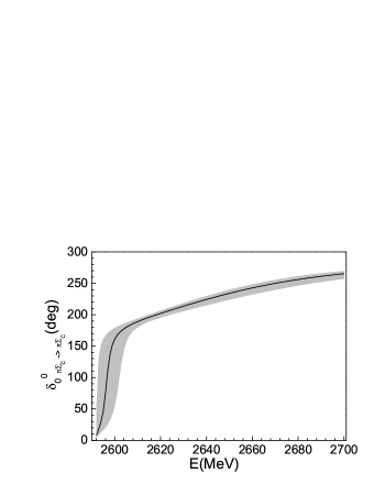
Figure 6: Phase shift for $\pi\Sigma_{c}$ scattering obtained from the two coupled channels unitary approach (solid line). The band is derived from the fits to the ”data” of Fig. 5 by using the potential of Eq. (14) with two channels.

At this point we want to improve the error analysis by introducing two new ingredients. The first one is to consider that the centroids of the data are not exactly on the exact curve, as it would correspond to actual lattice data. For this purpose we follow exactly the procedure done in Ref. misha and let the centroids move randomly within $\pm 5$ MeV from the exact point in the curves of Fig. 4. We then make a large number of runs and determine the new band of results. This is shown in Fig. 7. As we can see, the error band has increased a bit, by about $20\%$. We repeat the procedure allowing now the centroids moving randomly with $\pm 10$ MeV and we find that the band increases by an extra $20\%$ with respect to Fig. 7.

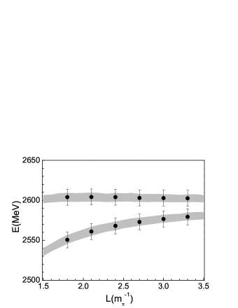
Figure 7: As in Fig. 5, but for the new fit with the error $\pm 5$ MeV for the centroids of the ’data’.

In a second step we also want to take into account the effects of using more freedom in the parameterization of the potential. This was discussed in Ref. mishakappa and was shown to be an extra source of uncertainty. We want to investigate what happens here. For this purpose we use a different parameterization of the potential guided by the terms that appear in Eq. (3). Thus, we take

$$V_{ij}= a_{ij}+b_{ij}(\sqrt{s}-(m_{\pi}+M_{\Sigma_{c}}))$$ (18)

$$+c_{ij}(s-(m_{\pi}+M_{\Sigma_{c}})^{2}),$$

hence, introducing three more parameters. We should note that with such large number of parameters one will not only be producing a smooth fit to the data, but the fit will also search situations to reproduce the fluctuations. This means we should consider the extra errors that come from this source certainly as an upper bound. The new results, considering also the dispersion of the centroids, are shown in Fig. 8 (note that we added also a new data point). As we can see, and similarly to what was fond in Ref. mishakappa , the error band has increased and now extends over the whole range of the assumed errors of the lattice data.

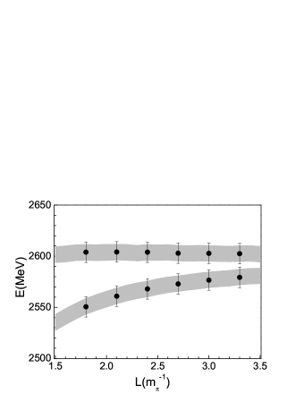
Figure 8: As in Fig. 5, but for the new fit by using the potential of Eq. (18) with two channels.

With the new potential we reevaluate the phase shifts with two channels as we have done for the Fig. 6, and the new results are shown in Fig. 9. The agreement with the exact results is good but the error band is now increased.

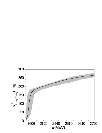
Figure 9: As in Fig. 6, but the band is derived from the fits to the ”data” of Fig. 8 by using the potential of Eq. (18) with two channels.

The analysis done here is based on the dominance of the $\pi\Sigma_{c}$ and $DN$ two body channels. The inclusion of three body channels makes the work technically much more involved, but has already been addressed formally in Ref. akakaitres . In the present case the $\Lambda_{c}(2595)$ resonance can decay into $\pi\Sigma_{c}$ but also in uncorrelated $\Lambda_{c}\pi\pi$. Fortunately the branching ratio in this channel is small and with large uncertainties, $18\pm 10\%$ pdg , that justifies its neglect in the present work. Should there be better data in the future on this branching ratio, and should one aim at a very accurate solution, some work along the lines of Ref. akakaitres would be advisable.

IV One channel analysis

Since the $\pi\Sigma_{c}$ channel is the only one open, one might be tempted to apply Lüscher’s approach with just one channel. One would be assuming implicitly that the effect of the $DN$ channel would be absorbed in the $\pi\Sigma_{c}$ potential. In such a case, the energy spectrum of Fig. 5 would be given by the poles of

$$T(E)=\frac{1}{V^{-1}-\tilde{G}(E)}$$ (19)

which gives us $V^{-1}=\tilde{G}$ for a value of $E$ eigenenergy of the box. For this energy, we can then write the scattering amplitude in infinite volume as

$$T(E)=\frac{1}{\tilde{G}(E)-G(E)}.$$ (20)

However, the direct application of this formula does not give information above the $\pi\Sigma_{c}$ threshold from the first level, since the eigenenergy values of the first level are below the $\pi\Sigma_{c}$ threshold. Besides, the second level is very stable and only gives us an energy point, with errors in the energy bigger than the width of the resonance. It is not possible to reconstruct the phase shifts in these circumstances. Because of this, it is more appropriate to consider all the data of one level, since one is then using the information on the correlation of these data. Then we fit all these data (five points) with the potential of Eq. (14) but with only the $\pi\Sigma_{c}$ channel (2 parameters). We get a good fit to the first level with $\chi^{2}_{min}=3.4\times 10^{-2}$. Then we use this potential to determine the infinite volume scattering amplitude $T$

$$T(E)=\frac{1}{V^{-1}-G(E)}.$$ (21)

The results for $\pi\Sigma_{c}$ phase shifts, with the lower band, are shown in Fig. 10. As we can see, the results obtained differ substantially from the exact results obtained with the two coupled channels, as shown in Fig. 10 by the solid line. We should note that, not even the scattering length is provided correctly.

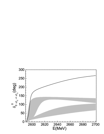
Figure 10: Phase shift $\delta^{0}_{0}$ for $\pi\Sigma_{c}$ scattering. Solid line: exact results obtained from the two coupled channels unitary approach. Lower band: derived from the fits to the first level ”data” of Fig. 5 by using the potential of Eq. (14) with only one $\pi\Sigma_{c}$ channel. Upper band: derived from the fits to the second level ”data” of Fig. 5 by using the potential of Eq. (14) with only one $\pi\Sigma_{c}$ channel.

Similarly we take now the second level in Fig. 5 and perform the same exercise. The best fit gives a larger $\chi^{2}_{min}=0.4$. The phase shifts obtained are also shown in Fig. 10 with the upper band. They are also in very bad agreement with the real results.

Besides, we can take the second level of Fig. 5 and analyze it with just the $DN$ channel. Then we cannot get the $\pi\Sigma_{c}$ phase shifts, but we see that the scattering amplitude obtained in the infinite volume by using Eq. (21) has a pole at $E=2601\pm 6$ MeV, corresponding to a $DN$ bound state. This is telling us that the second level of Fig. 5 is mostly tied to the $DN$ channel. One could guess that the stability of the energy level as a function of $L$ is showing the presence of a bound state, although this is not always the case, as shown in Ref. alberto . Yet, in the present case we have gone one step beyond, because our inverse analysis provides a parameter set for the potential from where we can determine poles, couplings and then test Eq. (7) for the compositeness condition. In the present case this renders a value of around $0.9$ for $-g^{2}_{DN}\frac{dG_{DN}}{dE}$, from where we conclude that the state corresponds essentially to a $DN$ bound state, weakly decaying into $\pi\Sigma_{c}$.

Once again we repeat the exercise done at the end of the former section and take into account at the same time the two effects considered here. Thus, we consider the dispersion of the centriods of the data and use the new parametrization of Eq. (18). In this case we have now three parameters in the potential. The new results can be seen in Fig. 11. We can see that the quality of the fit to the two levels is worse than the one obtained in Fig. 5 with two channels.

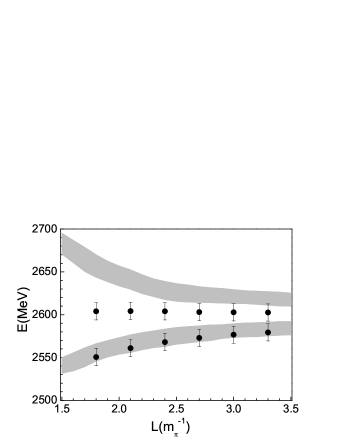
Figure 11: As in Fig. 5, but for the new fit with the error $\pm 5$ MeV for the centroids of the ’data’ and by using the potential of Eq. (18) with only one $\pi\Sigma_{c}$ channel.

Next, we evaluate the phase shifts with this new potential, fitted to the two levels, and the results can be seen in Fig. 12. Once again, we see that assuming just the $\pi\Sigma_{c}$ channel in the analysis leads to unrealistic $\pi\Sigma_{c}$ phase shifts.

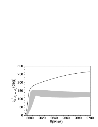
Figure 12: As in Fig. 10, but, the band is derived from the fits to the first two levels ”data” of Fig. 11 by using the potential of Eq. (18) with only one $\pi\Sigma_{c}$ channel.

In summary, we see the problems that arise when we try to use Lüscher’s approach for the interpretation of the lattice spectrum in a case where the relevance of a closed channel is huge, like in the present case. We also see that doing the fit analysis, that allows us to circumvent Lüscher’s approach, but using only one channel also fails to provide realistic phase shifts. The analysis with two channels shows here the tremendous power that the coupled channel approach has in this case.

V A test in terms of a CDD potential

On the other hand, there is the possibility that the nature of $\Lambda_{c}(2595)$ resonance could be a genuine state, not dynamically generated by the $DN$ interaction. For this purpose we have made a test introducing a different potential for the $DN$ interaction where a CDD pole (Castillejo, Dalitz, Dyson) cdd is introduced by hand. The potential for $DN$ interaction now is,

$$V=V_{M}+\frac{g^{2}_{CDD}}{\sqrt{s}-\sqrt{s_{CDD}}},$$ (22)

where $V_{M}$ is assumed to be energy independent and $g^{2}_{CDD}$, $s_{CDD}$ are the parameters of the CDD pole.

Like it has been done in Ref. alberto , from the above potential, we now find

$$1-\frac{g^{2}_{CDD}G^{2}}{(\sqrt{s}-\sqrt{s_{CDD}})^{2}\frac{dG}{dE}}=\frac{1}{1-Z},$$ (23)

with $Z$ the field renormalization constant for the genuine state, which accounts for the probability to have a genuine state.

We take the potential Eq. (22) with $V_{M}$ of the order of $10$ times smaller that the potential used for $V_{22}$, $\sqrt{s_{CDD}}$ corresponding to a 20 MeV below the mass of the $\Lambda_{c}(2595)$ and then $g^{2}_{CDD}=1.86$ such as to get the bound state at the mass of $\Lambda_{c}(2595)$. We find that at the pole of this state, from Eq. (23), we get $Z=0.96$, which shows that the introduction of a CDD pole as in in Eq. (22) is good enough to generate a genuine state.

The energy levels in the box with the potential of Eq. (22) for the $DN$ channel are shown in Fig. 13. As we can see, the levels are different from those obtained with the couple channel potential, which are shown in Fig. 4. It is clear that the determination of the levels with lattice calculations can differentiate between the two different types for the potentials.

Figure 13: Energy levels as functions of the cubic box size $L(m^{-1}_{\pi})$, derived from the potential of Eq. (22) for the $DN$ channel.

Next, we perform a fit, with a CDD potential Eq. (22) for $V_{22}$, to the first two levels of Fig. 4 that are obtained with the couple channel potential. We have taken also ten points over the curves and assumed $\pm 10$ MeV errors as we have done above. The best fitting results are: $g_{CDD}=91.4\pm 26.9$, $\sqrt{s_{CDD}}=8190\pm 1600$ MeV, and $V_{M}=1.23\pm 0.45$, with these values and their uncertainties, we can get now, at $E=2596$ MeV, $Z=0.15\pm 0.07$ from Eq. (23), which is in the order of $15\%$ with large error. This means around $85\%$ fraction of $\Lambda_{c}(2595)$ being dynamically generated. We should note that although we get a good fit with a potential that formally contains a CDD pole, the large value of the mass of the CDD pole renders the potential smooth, as in the case of the coupled channels, and the test tells us that the state corresponds to a dynamically generated one. We should also mention that we now only take two energy levels of Fig. 4 for fitting, this is why the best results have large errors. If we took more energy levels, we could determine these values with more precision. But our present result, $Z=0.15\pm 0.07$, suffices to show that from this limited information one can get valuable conclusions on the nature of the $\Lambda_{c}(2595)$ resonance, which is mostly a $DN$ bound state.

VI Summary

In this work, we study the interaction of the coupled channels $DN$ and $\pi\Sigma_{c}$ in an SU(4) extrapolation of the chiral unitary theory. The resulting interaction is used to reproduce the position of the $\Lambda_{c}(2595)$ resonance in the isospin zero $DN$ channel. Then we conclude that the $\Lambda_{c}(2595)$ is mostly a $DN$ bound state.

We then study the interaction of the coupled channels $DN$ and $\pi\Sigma_{c}$ in the finite volume. Energy levels in the finite box are evaluated. We assume that the results obtained would correspond to results given by lattice calculations. From there we address the inverse problem. We propose a rather general and realistic potential and, using two coupled channels, a fit to the synthetic data is made assuming some reasonable errors in the data. Then this potential is used in the infinite volume case, generating the $\pi\Sigma_{c}$ phase shifts within an error band around the original results. This part provides information for lattice QCD calculations about the accuracy in the energies of the spectrum needed to get a desired accuracy in the phase shifts.

A second part of the investigation was about the use of a one channel Lüscher’s approach, with just the open $\pi\Sigma_{c}$ channel, to induce $\pi\Sigma_{c}$ phase shifts from the finite volume spectrum. We found in this case that, due to the large weight of the closed $DN$ channel in this problem, the results obtained using Lüscher’s approach with just the $\pi\Sigma_{c}$ channel was of no use. Even more, making a fit analysis to the lattice data with just the $\pi\Sigma_{c}$ channel produced erroneous $\pi\Sigma_{c}$ phase shifts. Certainly one does not know a priori from the lattice QCD results whether two channels would be necessary in the analysis. However, we also showed that the results obtained from the analysis of the first two levels with just one channel were different to each other. This could be taken as a clear indication that at least two channels are needed in a realistic analysis of the lattice QCD results in such a case. The results from the chiral unitary approach, and the two channel formalism shown here, which can be trivially generalized to more channels, provide a good perspective to undertake future lattice QCD calculation in this sector. We also showed that the analysis done here, not only provides us with the $\pi\Sigma_{c}$ phase shifts and the presence of a bound state, but through the test of the sum rule of Eq. (7) (essentially Weinberg’s compositeness test), it also tells us that this bound state corresponds to a molecular state of a $DN$ system.

References

- (1) Y. Nakahara, M. Asakawa, T. Hatsuda, Phys. Rev. D60 (1999) 091503.
- (2) K. Sasaki, S. Sasaki and T. Hatsuda, Phys. Lett. B 623 (2005) 208.
- (3) N. Mathur, A. Alexandru, Y. Chen et al., Phys. Rev. D76 (2007) 114505.
- (4) S. Basak, R. G. Edwards, G. T. Fleming et al., Phys. Rev. D76 (2007) 074504.
- (5) J. Bulava, R. G. Edwards, E. Engelson et al., Phys. Rev. D82 (2010) 014507.
- (6) C. Morningstar, A. Bell, J. Bulava et al., AIP Conf. Proc. 1257 (2010) 779.
- (7) J. Foley, J. Bulava, K. J. Juge et al., AIP Conf. Proc. 1257 (2010) 789.
- (8) M. G. Alford and R. L. Jaffe, Nucl. Phys. B 578 (2000) 367.
- (9) T. Kunihiro, S. Muroya, A. Nakamura, C. Nonaka, M. Sekiguchi and H. Wada [SCALAR Collaboration], Phys. Rev. D 70 (2004) 034504.
- (10) F. Okiharu et al., arXiv: hep-ph/0507187.
- (11) H. Suganuma, K. Tsumura, N. Ishii and F. Okiharu, PoS LAT2005 (2006) 070; Prog. Theor. Phys. Suppl. 168 (2007) 168.
- (12) C. McNeile and C. Michael [UKQCD Collaboration], Phys. Rev. D 74 (2006) 014508.
- (13) A. Hart, C. McNeile, C. Michael and J. Pickavance [UKQCD Collaboration], Phys. Rev. D 74 (2006) 114504.
- (14) H. Wada, T. Kunihiro, S. Muroya, A. Nakamura, C. Nonaka and M. Sekiguchi, Phys. Lett. B 652 (2007) 250.
- (15) S. Prelovsek, C. Dawson, T. Izubuchi, K. Orginos and A. Soni, Phys. Rev. D 70 (2004) 094503.
- (16) S. Prelovsek, T. Draper, C. B. Lang, M. Limmer, K. F. Liu, N. Mathur and D. Mohler, Conf. Proc. C 0908171 (2009) 508; Phys. Rev. D 82 (2010) 094507.
- (17) H. -W. Lin et al. [ Hadron Spectrum Collaboration ], Phys. Rev. D79, (2009) 034502.
- (18) C. Gattringer, C. Hagen, C. B. Lang, M. Limmer, D. Mohler, A. Schafer, Phys. Rev. D79, (2009) 054501.
- (19) G. P. Engel et al. [ BGR [Bern-Graz-Regensburg] Collaboration ], Phys. Rev. D82, (2010) 034505.
- (20) M. S. Mahbub, W. Kamleh, D. B. Leinweber, A. O Cais, A. G. Williams, Phys. Lett. B693, (2010) 351-357.
- (21) R. G. Edwards, J. J. Dudek, D. G. Richards, S. J. Wallace, Phys. Rev. D84, (2011) 074508.
- (22) V. Bernard, U. -G. Meissner, A. Rusetsky, Nucl. Phys. B788, (2008) 1-20.
- (23) V. Bernard, M. Lage, U. -G. Meissner, A. Rusetsky, JHEP 0808, (2008) 024.
- (24) M. Döring, U. -G. Meissner, E. Oset, A. Rusetsky, Eur. Phys. J. A47, (2011) 139.
- (25) M. Lüscher, Commun. Math. Phys. 105 (1986) 153.
- (26) M. Lüscher, Nucl. Phys. B 354 (1991) 531.
- (27) C. Liu, X. Feng and S. He, Int. J. Mod. Phys. A 21, (2006) 847.
- (28) M. Lage, U. -G. Meissner and A. Rusetsky, Phys. Lett. B 681, (2009) 439.
- (29) V. Bernard, M. Lage, U. -G. Meissner and A. Rusetsky, JHEP 1101, (2011) 019.
- (30) M. T. Hansen and S. R. Sharpe, Phys. Rev. D 86 (2012) 016007.
- (31) R. A. Briceno and Z. Davoudi, arXiv: 1204.1110 [hep-lat].
- (32) M. Doring, J. Haidenbauer, U. -G. Meissner and A. Rusetsky, Eur. Phys. J. A 47, (2011) 163.
- (33) A. Martinez Torres, L. R. Dai, C. Koren, D. Jido and E. Oset, Phys. Rev. D 85, (2012) 014027.
- (34) E. E. Kolomeitsev, M. F. M. Lutz, Phys. Lett. B582, (2004) 39.
- (35) J. Hofmann, M. F. M. Lutz, Nucl. Phys. A733, (2004) 142.
- (36) F. -K. Guo, P. -N. Shen, H. -C. Chiang, R. -G. Ping, B. -S. Zou, Phys. Lett. B641, (2006) 278.
- (37) D. Gamermann, E. Oset, D. Strottman, M. J. Vicente Vacas, Phys. Rev. D76, (2007) 074016.
- (38) M. Doring and U. G. Meissner, JHEP 1201, (2012 009).
- (39) J. Hofmann and M. F. M. Lutz, Nucl. Phys. A 763, (2005) 90.
- (40) T. Mizutani and A. Ramos, Phys. Rev. C 74, (2006) 065201.
- (41) L. Tolos, A. Ramos, and T. Mizutani, Phys. Rev. C 77, (2008) 015207 .
- (42) C. Garcia-Recio, V. K. Magas, T. Mizutani, J. Nieves, A. Ramos, L. L. Salcedo, and L. Tolos, Phys. Rev. D 79, (2009) 054004.
- (43) D. Gamermann, http://ific.uv.es/nucth/tesis-DanGam.pdf.
- (44) Jia-Jun Wu, R. Molina, E. Oset and Bing-Song Zou, Phys. Rev. Lett. 105, (2010) 232001.
- (45) D. Gamermann, J. Nieves, E. Oset, E. Ruiz Arriola, Phys. Rev. D81, (2010) 014029.
- (46) S. Weinberg, Phys. Rev. 137, (1965) B677.
- (47) T. Sekihara, T. Hyodo and D. Jido, Phys. Rev. C 83, (2011) 055202.
- (48) J. A. Oller and E. Oset, Nucl. Phys. A 620, (1997) 438.
- (49) J. A. Oller and U. G. Meissner, Phys. Lett. B 500, (2001) 263.
- (50) For tabulated numbers and further references see, e.g., The On-Line Encyclopedia of Integer Sequences, http://oeis.org/A005875.
- (51) J. A. Oller, E. Oset and J. R. Pelaez, Phys. Rev. D 59 (1999) 074001 [Erratum-ibid. D 60 (1999) 099906] [Erratum-ibid. D 75 (2007) 099903].
- (52) K. Polejaeva and A. Rusetsky, Eur. Phys. J. A 48, (2012)67.
- (53) J. Beringer et al. (Particle Data Group), Phys. Rev. D86, (2012) 010001.
- (54) L. Castillejo, R.H. Dalitz, and F.J. Dyson, Phys. Rev. (101), (1956) 453.