An Upper Bound to the Marginal PDF of the Ordered Eigenvalues of Wishart Matrices^†

Abstract

Diversity analysis of a number of Multiple-Input Multiple-Output (MIMO) applications requires the calculation of the expectation of a function whose variables are the ordered multiple eigenvalues of a Wishart matrix. In order to carry out this calculation, we need the marginal pdf of an arbitrary subset of the ordered eigenvalues. In this letter, we derive an upper bound to the marginal pdf of the eigenvalues. The derivation is based on the multiple integration of the well-known joint pdf, which is very complicated due to the exponential factors of the joint pdf. We suggest an alternative function that provides simpler calculation of the multiple integration. As a result, the marginal pdf is shown to be bounded by a multivariate polynomial with a given degree. After a standard bounding procedure in a Pairwise Error Probability (PEP) analysis, by applying the marginal pdf to the calculation of the expectation, the diversity order for a number of MIMO systems can be obtained in a simple manner. Simulation results that support the analysis are presented.

I Introduction

In wireless communications, the Wishart matrix arises from the MIMO transmission environment, where the channel matrix is modeled as complex Gaussian, as in the Rayleigh fading model [1]. In particular, if the channel matrix is available at the transmitter as well as at the receiver, the beamforming matrices can be obtained from the singular value decomposition (SVD) of the channel matrix to build the diagonalizing structure, known to be optimal to maximize the performance [2]. In the uncoded version of this multiple beamforming scheme, the diversity order, an important performance measure of MIMO systems at the high signal-to-noise ratio regime, is determined by the subchannel with the smallest eigenvalue of the Wishart matrix [3], [4], [5]. In general, the diversity order is calculated from the PEP, expressed as $E\left[\kappa(\mu_{l})\right]$, where $\kappa(\mu_{l})$ is a function of the $l^{th}$ ordered eigenvalue $\mu_{l}$, and $E[\,\cdot\,]$ is the expectation operator. In order to carry out this calculation, we need to find the marginal pdf of the single eigenvalue $\mu_{l}$ of the Wishart matrix. A first order polynomial expansion is used to derive the simple closed form expression of the marginal pdf in [4] and [6], while the more accurate expression as the sums of terms of the form $\mu_{l}^{x}e^{y\mu_{l}}$ is provided in [5]. The resulting diversity order of multiple beamforming with the $l^{th}$ eigenvalue involved is $(N-l+1)(M-l+1)$ where $N$ and $M$ are the number of transmit and receive antennas, respectively [3], [4].

The average PEP between two codewords in the coded multiple beamforming scheme, on the other hand, requires the calculation of the expectation $E\left[\phi(\mu_{1},\cdots,\mu_{Y})\right]$, where $\phi(\cdot)$ is a function with multiple ordered eigenvalues involved [7]. For the pairwise codewords whose corresponding function $\phi(\cdot)$ includes all of the singular values available from the SVD of the channel matrix, authors in [7] calculated the diversity order from the simple closed form expression of the average PEP, by making use of the fact that the sum of all ordered eigenvalues follows a chi-squared distribution. If $\phi(\cdot)$ is composed of a subset of the ordered eigenvalues, the calculation of the expectation needs the marginal pdf of the eigenvalues. The closed form expressions of consecutive and an arbitrary subset of ordered eigenvalues are given in [8], while the expressions for unordered eigenvalues are provided in [9] and [10]. A difficulty exists in determining an analytical diversity figure with these prior approaches. They are typically in the form of a product of integrals to be calculated, and consist of the incomplete Gamma functions that enable numerical evaluation, but make the analysis difficult.

In this letter, we propose a methodology to calculate an upper bound to the marginal pdf of the ordered eigenvalues. Then, we derive the diversity order by using the upper bound to the marginal pdf. Since the direct calculation of the marginal pdf is very complicated due to the multiple integration of the joint pdf which has the exponential function, we suggest an alternative function as a substitute for the joint pdf to simplify the multiple integration. The resulting diversity order is $(N-p_{1}+1)(M-p_{1}+1)$ where $p_{1}$ is the index to indicate the best among the eigenvalues appearing in the $\phi(\cdot)$ function.

II Problem Statement

The elements of the MIMO channel $\mathbf{H}\in\mathbb{C}^{M\times N}$ are assumed to be Gaussian with zero mean and unit variance. In addition, the covariance matrix, which is defined as $\mathbf{V}_{j}=E[\mathbf{h}_{j}\mathbf{h}_{j}^{\dagger}]$ where $\mathbf{h}_{j}$ is the $j^{th}$ column vector of $\mathbf{H}$, and ${\dagger}$ stands for conjugate transpose, satisfies $\mathbf{V}_{j}=\mathbf{I}$ for all $j$. Based on the assumption above, the matrix $\mathbf{HH}^{{\dagger}}$ is called uncorrelated central Wishart matrix [5]. The $i^{th}$ eigenvalue of $\mathbf{HH}^{{\dagger}}$, denoted by $\mu_{i}$, is sorted such that $\mu_{i}>\mu_{j}$ for $i<j$. Throughout this letter, we use $X$ and $Y$ as $X=\max(N,M)$, and $Y=\min(N,M)$.

The average pairwise error probability that the receiver decides $\mathbf{\hat{c}}$ instead of $\mathbf{c}$ as the transmitted signal is upper bounded by [7]

$$\mathrm{Pr}\left(\mathbf{c}\rightarrow\mathbf{\hat{c}}\right)\leq E\left[\exp\left(-\gamma\sum\limits_{j=1}^{Y}\alpha_{j}\mu_{j}\right)\right]$$ (1)

where $\gamma$ is the signal-to-noise ratio, and $\alpha_{j}$ is a given non-negative real value. We note that a bound of this form can be obtained for a number of MIMO SVD systems, e.g., [11], [12], [13], [14]. Let’s define $\alpha_{min}$ as the minimum among the nonzero $\alpha$ values. Using the inequality $\sum_{j=1}^{Y}\alpha_{j}\mu_{j}\geq\alpha_{min}\sum_{j=1,\alpha_{j}\neq 0}^{Y}\mu_{j}$, we rewrite (1) as

$$\mathrm{Pr}\left(\mathbf{c}\rightarrow\mathbf{\hat{c}}\right)\leq E\left[\exp\left(-\gamma\alpha_{min}\sum\limits_{k=1}^{K}\mu_{p_{k}}\right)\right]$$ (2)

where $p_{k}$ is the $k^{th}$ element of a vector $\mathbf{p}=[p_{1}\,\cdots\,p_{K}]^{T}$ whose elements are the indices corresponding to non-zero $\alpha$, i.e., $\alpha_{p_{k}}\neq 0$. Similarly, $\mathbf{s}=[s_{1}\,\cdots\,s_{(Y-K)}]^{T}$ is defined as a vector whose elements are the indices $k$ such that $\alpha_{s_{k}}=0$. The vectors $\mathbf{p}$ and $\mathbf{s}$ are sorted in increasing order. To calculate (2), we need the marginal pdf of the $K$ eigenvalues by calculating the multiple integration over the domain $\mathcal{D}_{\mathbf{s}}$

$$f\left(\mu_{p_{1}},\cdots,\mu_{p_{K}}\right)=\\ \int\cdots\int_{\mathcal{D}_{\mathbf{s}}}\rho\left(\mu_{1},\cdots,\mu_{Y}\right)\,d\mu_{s_{(Y-K)}}\,\cdots\,d\mu_{s_{1}}.$$ (3)

The joint pdf of the ordered strictly positive eigenvalues of the uncorrelated central Wishart matrices $\rho\left(\mu_{1},\cdots,\mu_{Y}\right)$ in (3) is available in the literature [1], [15] as

$$\rho\left(\mu_{1},\cdots,\mu_{Y}\right)=\psi\left(\mu_{1},\cdots,\mu_{Y}\right)e^{-\sum\limits_{j=1}^{Y}\mu_{j}}$$ (4)

where the polynomial $\psi\left(\mu_{1},\cdots,\mu_{Y}\right)$ is

$$\psi\left(\mu_{1},\cdots,\mu_{Y}\right)=\prod^{Y}_{i=1}\mu_{i}^{X-Y}\prod^{Y}_{j>i}\left(\mu_{i}-\mu_{j}\right)^{2}.$$ (5)

Because we are interested in the exponent of $\gamma$, a constant multiplier, which appears in the literature, and is irrelevant to the exponent of $\gamma$, is ignored in (5) for brevity.

The closed form expression of the marginal pdf can be calculated by evaluating (3). However, this evaluation is complicated due to the multiple integration of the product of the polynomial and the exponential function in (3)-(5). Alternatively, we will now develop a method to get a simple expression for an upper bound to the marginal pdf. Then, we will use the upper bound to calculate (2).

III An Upper Bound to the Marginal PDF

The complexity of the multiple integration to calculate the marginal pdf in (3) mainly comes from the fact that the elementary integration inside the multiple integration, $\int_{0}^{x}y^{m}e^{-y}dy$, generates a large number of terms of the form $x^{n}e^{-x}$ for large $m$, i.e.,

$$\int_{0}^{x}y^{m}e^{-y}dy =\left[-y^{m}e^{-y}\right|_{0}^{y=x}+m\int_{0}^{x}y^{m-1}e^{-y}dy$$

$$=-e^{-x}(x^{m}+mx^{m-1}$$ (6)

$$\qquad+m(m-1)x^{m-2}+\cdots+m!)+m!.$$

However, if we remove the exponential function from the elementary integration, the integration produces only one term, resulting in a much simpler multiple integration. In addition, since the eigenvalues of the Wishart matrix are positive and real, $e^{-\mu_{i}}\leq 1$ holds true for any $i$. This idea leads to a simple result of the elementary integration as

$$\int_{0}^{x}y^{m}e^{-y}dy\leq\frac{1}{m+1}x^{m+1}.$$ (7)

To apply the idea above to the calculation of the marginal pdf, we introduce an alternative function

$$\hat{\rho}\left(\mu_{1},\cdots,\mu_{Y}\right)=\\ \left\{\begin{array}[]{ll}\psi\left(\mu_{1},\cdots,\mu_{Y}\right)e^{-\left(\mu_{1}+\sum\limits_{k=1}^{K}\mu_{p_{k}}\right)}\\ &\textrm{if $\alpha_{1}=0$}\\ \psi\left(\mu_{1},\cdots,\mu_{Y}\right)e^{-\sum\limits_{k=1}^{K}\mu_{p_{k}}}&\textrm{if $\alpha_{1}>0$}\end{array}\right.$$ (8)

where the exponential factors irrelevant to the variables of integration are removed, except $\mu_{1}$ which is kept in the case of $\alpha_{1}=0$. The reason for keeping $\mu_{1}$ will be explained later. Correspondingly, let’s define $\hat{f}\left(\mu_{p_{1}},\cdots,\mu_{p_{K}}\right)$ in a similar fashion to (3) with $\rho\left(\mu_{1},\cdots,\mu_{Y}\right)$ replaced by $\hat{\rho}\left(\mu_{1},\cdots,\mu_{Y}\right)$, that is,

$$\hat{f}\left(\mu_{p_{1}},\cdots,\mu_{p_{K}}\right)=\\ \int\cdots\int_{\mathcal{D}_{\mathbf{s}}}\hat{\rho}\left(\mu_{1},\cdots,\mu_{Y}\right)d\mu_{s_{(Y-K)}}\,\cdots\,d\mu_{s_{1}}.$$ (9)

We see that $\rho\left(\mu_{1},\cdots,\mu_{Y}\right)\leq\hat{\rho}\left(\mu_{1},\cdots,\mu_{Y}\right)$ for either the case of $\alpha_{1}=0$ or $\alpha_{1}>0$, and therefore, $f\left(\mu_{p_{1}},\cdots,\mu_{p_{K}}\right)\leq\hat{f}\left(\mu_{p_{1}},\cdots,\mu_{p_{K}}\right)$, where $\hat{f}\left(\mu_{p_{1}},\cdots,\mu_{p_{K}}\right)$ has a simpler expression. We will employ (9) to calculate our bound in the next subsections.

III-1 For $\alpha_{1}=0$

Since some factors of $\hat{\rho}\left(\mu_{1},\cdots,\mu_{Y}\right)$ are irrelevant to the variables of integration, they can be moved out. By defining a polynomial $g\left(\mu_{p_{1}},\cdots,\mu_{p_{K}}\right)$

$$g\left(\mu_{p_{1}},\cdots,\mu_{p_{K}}\right)=\prod^{K}_{k=1}\mu_{p_{k}}^{X-Y}\prod^{K}_{j>k}\left(\mu_{p_{k}}-\mu_{p_{j}}\right)^{2},$$ (10)

we rewrite (9) as

$$\hat{f}\left(\mu_{p_{1}},\cdots,\mu_{p_{K}}\right)=g\left(\mu_{p_{1}},\cdots,\mu_{p_{K}}\right)e^{-\sum\limits_{k=1}^{K}\mu_{p_{k}}}\\ \times\int_{0}^{\infty}e^{-\mu_{1}}\int_{0}^{\mu_{s_{2}-1}}\cdots\int_{0}^{\mu_{s_{(Y-K)}-1}}\\ \times\frac{\psi\left(\mu_{1},\cdots,\mu_{Y}\right)}{g\left(\mu_{p_{1}},\cdots,\mu_{p_{K}}\right)}d\mu_{s_{(Y-K)}}\cdots d\mu_{s_{2}}d\mu_{1}$$ (11)

where $\frac{\psi\left(\mu_{1},\cdots,\mu_{Y}\right)}{g\left(\mu_{p_{1}},\cdots,\mu_{p_{K}}\right)}$ is a polynomial of the remained factors, and $d\mu_{s_{1}}$ is replaced by $d\mu_{1}$ since $s_{1}=1$ for $\alpha_{1}=0$. The multiple integration of $\frac{\psi\left(\mu_{1},\cdots,\mu_{Y}\right)}{g\left(\mu_{p_{1}},\cdots,\mu_{p_{K}}\right)}$ over the variables $\mu_{s_{(Y-K)}}$, $\cdots$, $\mu_{s_{2}}$ results in an intermediate polynomial whose terms are composed of the variables $\mu_{1}$, $\mu_{p_{1}}$, $\cdots$, $\mu_{p_{K}}$. In other words, the intermediate polynomial is the sum of the terms of the form as $\mu_{p_{1}}^{x_{1}}\times\cdots\times\mu_{p_{K}}^{x_{K}}\int_{0}^{\infty}\mu_{1}^{y}e^{-\mu_{1}}d\mu_{1}$. The final integration of the intermediate polynomial over $\mu_{1}$ leaves a polynomial with the variables $\mu_{p_{1}}$, $\cdots$, $\mu_{p_{K}}$ since $\int_{0}^{\infty}\mu_{1}^{y}e^{-\mu_{1}}d\mu_{1}=y!$. It should now be clear why we keep $e^{-\mu_{1}}$ in $\hat{\rho}\left(\mu_{1},\cdots,\mu_{Y}\right)$. The absence of this factor would have led the integration to diverge.

Defining $h_{1}\left(\mu_{p_{1}},\cdots,\mu_{p_{K}}\right)$ as the result of the multiple integration, we rewrite (11) as

$$\hat{f}\left(\mu_{p_{1}},\cdots,\mu_{p_{K}}\right)=r_{1}\left(\mu_{p_{1}},\cdots,\mu_{p_{K}}\right)e^{-\sum\limits_{k=1}^{K}\mu_{p_{k}}}$$ (12)

where the polynomial $r_{1}\left(\mu_{p_{1}},\cdots,\mu_{p_{K}}\right)$ is defined as

$$r_{1}\left(\mu_{p_{1}},\cdots,\mu_{p_{K}}\right)=\\ h_{1}\left(\mu_{p_{1}},\cdots,\mu_{p_{K}}\right)\times g\left(\mu_{p_{1}},\cdots,\mu_{p_{K}}\right).$$ (13)

III-2 For $\alpha_{1}>0$

Using the polynomial $g\left(\mu_{p_{1}},\cdots,\mu_{p_{K}}\right)$ in (10), we rewrite (9) in this case as

$$\hat{f}\left(\mu_{p_{1}},\cdots,\mu_{p_{K}}\right)=g\left(\mu_{p_{1}},\cdots,\mu_{p_{K}}\right)e^{-\sum\limits_{k=1}^{K}\mu_{p_{k}}}\\ \times\int_{0}^{\mu_{s_{1}-1}}\int_{0}^{\mu_{s_{2}-1}}\cdots\int_{0}^{\mu_{s_{(Y-K)}-1}}\\ \times\frac{\psi\left(\mu_{1},\cdots,\mu_{Y}\right)}{g\left(\mu_{p_{1}},\cdots,\mu_{p_{K}}\right)}d\mu_{s_{(Y-K)}}\cdots d\mu_{s_{2}}d\mu_{s_{1}}$$ (14)

where $\frac{\psi\left(\mu_{1},\cdots,\mu_{Y}\right)}{g\left(\mu_{p_{1}},\cdots,\mu_{p_{K}}\right)}$ is the same kind of polynomial that is described in the previous subsection. The multiple integration results in a polynomial of the variables $\mu_{p_{1}}$, $\cdots$, $\mu_{p_{K}}$ without diverging since the last integration is not involved with infinity. By defining $h_{2}\left(\mu_{p_{1}},\cdots,\mu_{p_{K}}\right)$ as the result of the multiple integration of (14), we get $\hat{f}\left(\mu_{p_{1}},\cdots,\mu_{p_{K}}\right)$ as

$$\hat{f}\left(\mu_{p_{1}},\cdots,\mu_{p_{K}}\right)=r_{2}\left(\mu_{p_{1}},\cdots,\mu_{p_{K}}\right)e^{-\sum\limits_{k=1}^{K}\mu_{p_{k}}}$$ (15)

where $r_{2}\left(\mu_{p_{1}},\cdots,\mu_{p_{K}}\right)$ is defined as

$$r_{2}\left(\mu_{p_{1}},\cdots,\mu_{p_{K}}\right)=\\ h_{2}\left(\mu_{p_{1}},\cdots,\mu_{p_{K}}\right)\times g\left(\mu_{p_{1}},\cdots,\mu_{p_{K}}\right).$$ (16)

The polynomials $r_{1}\left(\mu_{p_{1}},\cdots,\mu_{p_{K}}\right)$ and $r_{2}\left(\mu_{p_{1}},\cdots,\mu_{p_{K}}\right)$ are multivariate polynomials with many terms. It is worthwhile to focus on the smallest degree of the terms because it plays an important role in determining the behavior of (1) in the high signal-to-noise ratio regime. The mathematical analysis of the behavior will be described in Section IV with the help of the next Theorem.

Theorem 1

The smallest degree of the multivariate polynomial $r_{1}\left(\mu_{p_{1}},\cdots,\mu_{p_{K}}\right)$ or $r_{2}\left(\mu_{p_{1}},\cdots,\mu_{p_{K}}\right)$ is $(N-p_{1}+1)(M-p_{1}+1)-K$.

Proof:

See Appendix A. ∎

In the case of the single eigenvalue where $K=1$, and $p_{1}=l$, Theorem 1 states that the smallest degree of $\mu_{l}$ is $(N-l+1)(M-l+1)-1$. This generalizes the result of the first order expansion in [4], [6] to calculate the marginal pdf of the $l^{th}$ eigenvalue.

IV Calculation of the Expectation

According to the analysis in Section III, the marginal pdf $f\left(\mu_{p_{1}},\cdots,\mu_{p_{K}}\right)$ is upper bounded by the general expression

$$f\left(\mu_{p_{1}},\cdots,\mu_{p_{K}}\right)\leq r\left(\mu_{p_{1}},\cdots,\mu_{p_{K}}\right)e^{-\sum\limits_{k=1}^{K}\mu_{p_{k}}}$$

where $r\left(\mu_{p_{1}},\cdots,\mu_{p_{K}}\right)$ is a polynomial with the smallest degree of $(N-p_{1}+1)(M-p_{1}+1)-K$. We are now ready to obtain an upper bound to (2) by calculating

$$E \left[\exp\left(-\gamma\alpha_{min}\sum\limits_{k=1}^{K}\mu_{p_{k}}\right)\right]$$

$$=\int\cdots\int_{\mathcal{D}_{\mathbf{p}}}\exp\left(-\gamma\alpha_{min}\sum\limits_{k=1}^{K}\mu_{p_{k}}\right)$$

$$\qquad\times f\left(\mu_{p_{1}},\cdots,\mu_{p_{K}}\right)d\mu_{p_{K}}\cdots d\mu_{p_{1}}$$ (17)

$$\leq\int_{0}^{\infty}\cdots\int_{0}^{\mu_{p_{K-1}}}r\left(\mu_{p_{1}},\cdots,\mu_{p_{K}}\right)$$

$$\qquad\times e^{-(1+\gamma\alpha_{min})\sum\limits_{k=1}^{K}\mu_{p_{k}}}d\mu_{p_{K}}\cdots d\mu_{p_{1}}$$

where $\mathcal{D}_{\mathbf{p}}$ is the domain of integration. Note that $e^{-(1+\gamma\alpha_{min})\sum_{k=1}^{K}\mu_{p_{k}}}<e^{-\gamma\alpha_{min}\sum_{k=1}^{K}\mu_{p_{k}}}$. In Theorem 2, we provide the result of the multiple integration of a term whose degree is $\sum_{k}\beta_{k}$.

Theorem 2

For a multivariate term with variables $\theta_{i}$ for $i=1,\cdots,K$ whose exponent, denoted by $\beta_{i}$, is a non-negative integer, the multiple integration in the domain $\infty>\theta_{1}>\theta_{2}>\cdots>\theta_{K}>0$ is

$$\int_{0}^{\infty}\cdots\int_{0}^{\theta_{K-1}}\theta_{1}^{\beta_{1}}\cdots\theta_{K}^{\beta_{K}}e^{-\omega\sum\limits_{k=1}^{K}\theta_{k}}d\theta_{K}\cdots d\theta_{1}=\\ \zeta\omega^{-\left(K+\sum\limits_{k=1}^{K}\beta_{k}\right)}$$ (18)

where $\zeta$ is a constant.

Proof:

See Appendix B. ∎

Since the polynomial $r\left(\mu_{p_{1}},\cdots,\mu_{p_{K}}\right)$ is the sum of a number of terms with different degrees, the result of (17) is also the sum of the terms of $(\gamma\alpha_{min})$ whose exponent obeys Theorem 2. For large $\gamma$, it is easy to see that the overall sum is dominated by the term with the smallest degree of $\gamma^{-1}$. Theorem 2 indicates that the smallest degree of $\gamma^{-1}$ results from the smallest degree of $r\left(\mu_{p_{1}},\cdots,\mu_{p_{K}}\right)$. Therefore, we conclude that (1) is upper bounded by

$$E\left[\exp\left(-\gamma\sum\limits_{j=1}^{Y}\alpha_{j}\mu_{j}\right)\right]\leq\\ \eta\left(\gamma\alpha_{min}\right)^{-(N-p_{1}+1)(M-p_{1}+1)}$$ (19)

where $\eta$ is a constant, and irrelevant to $\gamma$.

V Simulation Results

Fig. 1 shows the calculation of (1) where $N=M=3$, with several specific $\alpha$ values through a Monte-Carlo simulation. The legend represents the $\alpha$ values as a vector notation $[\alpha_{1}\cdots\alpha_{S}]$. Three dotted straight lines are the asymptotes whose exponents correspond to $1$, $4$, and $9$. The curves of the $\alpha$ values $[1\,\,0\,\,0]$, $[0.1\,\,0\,\,1]$, and $[3\,\,0\,\,5]$, whose $p_{1}$ is $1$, are parallel to the asymptote of $(3-1+1)(3-1+1)=9$. By comparing the slopes of the other curves with the asymptotes, we see that the analysis is supported by the simulation.

Figure 1: Simulation results together with asymptotic diversity orders that show the validity of the technique for $N=M=3$. The vector $[\alpha_{1}\;\alpha_{2}\;\alpha_{3}]$ is provided in the legend. Note the importance of the first $\alpha_{i}$ equal to zero in determining the diversity order.

Fig. 2 depicts the simulation result of $N=M=4$. The dotted lines are the asymptotes of the exponents $4$, $9$ and $16$. A comparison of a slope with the asymptote reveals that simulation matches the analysis. Note that even though $\alpha$ corresponding to the smallest eigenvalue is $100$ times that of the best eigenvalue, the slope is determined by the best eigenvalue.

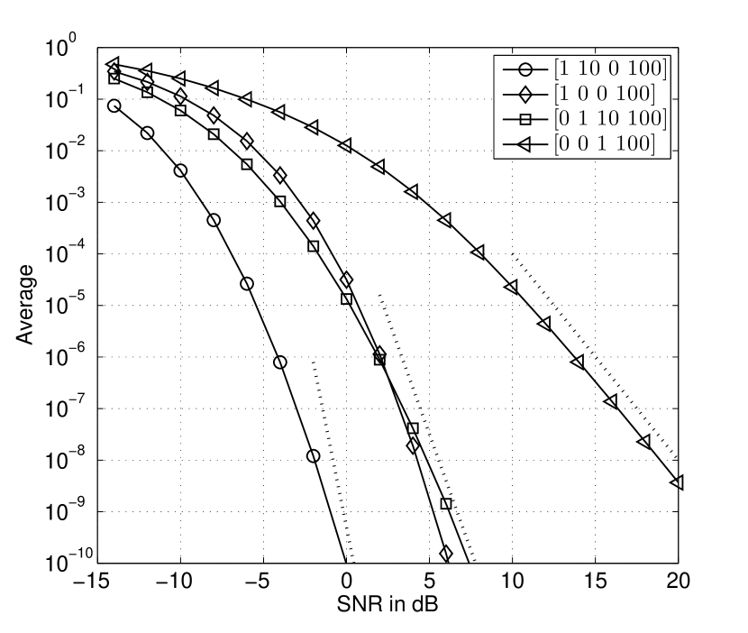
Figure 2: Simulation results together with asymptotic diversity orders that show the validity of the technique for $N=M=4$. Note the accuracy of the technique even if the first nonzero eigenvalue may be much smaller than the successive ones.

VI Conclusion

We derived an upper bound to the marginal pdf of the ordered eigenvalues of a complex central Wishart matrix. Such matrices arise in the analysis of MIMO SVD systems. Our bound employs an alternative function to simplify the multiple integration of the pdf.

For MIMO systems employing SVD, a standard bounding technique provides a simple bound such as (1), see e.g., [3], [7],[11], [12], [13], [14]. By applying our result to the calculation of the expectation, one can calculate the diversity order $(N-p_{1}+1)(M-p_{1}+1)$ in the high signal-to-noise ratio regime for a system where $N$ and $M$ are the number of transmit and receive antennas, respectively, and $p_{1}$ is the index to the smallest nonzero weight value in a PEP analysis. Simulation results provided here and elsewhere support the validity of the technique for a variety of MIMO SVD systems with a number of different parameters, see, e.g., [11], [12], [13], [14].

Appendix A Proof of Theorem 1

A-1 For $\alpha_{1}=0$

Since $r_{1}\left(\mu_{p_{1}},\cdots,\mu_{p_{K}}\right)$ is a product of two polynomials as shown in (13), the smallest degree of $r_{1}\left(\mu_{p_{1}},\cdots,\mu_{p_{K}}\right)$ is the sum of the smallest degrees of each polynomial $g\left(\mu_{p_{1}},\cdots,\mu_{p_{K}}\right)$ and $h_{1}\left(\mu_{p_{1}},\cdots,\mu_{p_{K}}\right)$. Let’s define $D_{g,smallest}$ as the smallest degree of the polynomial $g\left(\mu_{p_{1}},\cdots,\mu_{p_{K}}\right)$. It is easily found that all of the terms in (10) have the same degree. Therefore,

$$D_{g,smallest}=K(X-Y)+K(K-1)$$ (20)

where the degree of $K(X-Y)$ is contributed by the $K$ factors of the form $\mu_{p_{k}}^{X-Y}$, and $K(K-1)$ comes from the $\binom{K}{2}$ factors in the form of $\left(\mu_{p_{k}}-\mu_{p_{j}}\right)^{2}$.

To calculate the smallest degree of the polynomial $h_{1}\left(\mu_{p_{1}},\cdots,\mu_{p_{K}}\right)$, we need to know the degree of the polynomial $\frac{\psi\left(\mu_{1},\cdots,\mu_{Y}\right)}{g\left(\mu_{p_{1}},\cdots,\mu_{p_{K}}\right)}$. The polynomial $\psi\left(\mu_{1},\cdots,\mu_{Y}\right)$ in (5) has $Y$ factors of the form $\mu_{i}^{X-Y}$ and $\binom{Y}{2}$ factors of the form $\left(\mu_{i}-\mu_{j}\right)^{2}$. The division by $g\left(\mu_{p_{1}},\cdots,\mu_{p_{K}}\right)$ makes the common factors eliminated, leaving $(Y-K)$ factors of the form $\mu_{i}^{X-Y}$ and $(\binom{Y}{2}-\binom{K}{2})$ factors of the form $\left(\mu_{i}-\mu_{j}\right)^{2}$. Hence, the resulting polynomial $\frac{\psi\left(\mu_{1},\cdots,\mu_{Y}\right)}{g\left(\mu_{p_{1}},\cdots,\mu_{p_{K}}\right)}$ has degree

$$D_{h_{1},org}=(Y-K)(X-Y)+Y(Y-1)-K(K-1)$$ (21)

for all of the terms of the polynomial.

Obviously, there exists an integer $\epsilon$ such that $s_{\epsilon}<p_{1}<s_{\epsilon+1}$ since $p_{1}>1$. The integration over $\mu_{i}$ for $1\leq i\leq s_{\epsilon}$ in (11) makes these variables vanish because of the integration to infinity due to $\mu_{1}$, while that over the other $\mu_{j}$ for $s_{\epsilon+1}\leq j\leq s_{(Y-K)}$ converts those variables into the variables $\mu_{p_{1}},\cdots,\mu_{p_{K}}$. In the meanwhile, all the terms in $\frac{\psi\left(\mu_{1},\cdots,\mu_{Y}\right)}{g\left(\mu_{p_{1}},\cdots,\mu_{p_{K}}\right)}$ have different distributions on the degrees of the individual variables although they have the same degree as an entire term. Therefore, the smallest degree of $h_{1}\left(\mu_{p_{1}},\cdots,\mu_{p_{K}}\right)$ is determined by the term which has the largest degree of those vanishing variables of $\frac{\psi\left(\mu_{1},\cdots,\mu_{Y}\right)}{g\left(\mu_{p_{1}},\cdots,\mu_{p_{K}}\right)}$. It is not necessary to find all the terms with the largest degree of the vanishing variables. Instead, we can see that one of those terms, whose degree is $D_{h_{1},org}$, includes the factors

$$\prod\limits_{i=1}^{p_{1}-1}\mu_{i}^{X-Y}\prod\limits_{j>i}^{Y}\mu_{i}^{2}.$$ (22)

In this case, the degree corresponding to the vanishing variables in (22) is

$$D_{h_{1},vanishing}=(p_{1}-1)(X-Y)\\ +2Y(p_{1}-1)-p_{1}(p_{1}-1)$$ (23)

where $(p_{1}-1)(X-Y)$ is contributed by the $(p_{1}-1)$ factors of the form $\mu_{i}^{X-Y}$, and the rest of the degrees are calculated from the factors of the form $\mu_{i}^{2}$.

Finally, the integration over $\mu_{j}$ for $s_{\epsilon+1}\leq j\leq s_{(Y-K)}$ accumulates the degree of the current variables as well as the previous variables belonging to $\mathbf{s}$. Hence, the degree of the variables $\mu_{k}$ for $k\geq p_{1}$ is kept during the multiple integration. In addition, during each integration of $\mu_{j}$ for $s_{\epsilon+1}\leq j\leq s_{(Y-K)}$, the degree increases by $1$ due to the fact that $\int_{0}^{\mu_{i}}\mu_{i+1}^{n}d\mu_{i+1}=\mu_{i}^{n+1}/(n+1)$. Since $s_{\epsilon}$ variables from the original $(Y-K)$ variables of integration vanished in $h_{1}\left(\mu_{p_{1}},\cdots,\mu_{p_{K}}\right)$, the degree to be added is

$$D_{h_{1},added}=Y-K-p_{1}+1$$ (24)

where $s_{\epsilon}$ is replaced by $(p_{1}-1)$. The smallest degree of $r_{1}\left(\mu_{p_{1}},\cdots,\mu_{p_{K}}\right)$ can be calculated as

$$D_{r_{1},smallest} =D_{g,smallest}+D_{h_{1},smallest}$$

$$=D_{g,smallest}$$

$$\quad+\left(D_{h_{1},org}-D_{h_{1},vanishing}+D_{h_{1},added}\right)$$

$$=(X-p_{1}+1)(Y-p_{1}+1)-K$$ (25)

where $D_{h_{1},org}-D_{h_{1},vanishing}$ stands for the degree which is kept during the integration over $\mu_{j}$ for $s_{\epsilon+1}\leq j\leq s_{(Y-K)}$. If $X$ is equal to $N$, then $Y$ is $M$, and vice versa, the smallest degree is $(N-p_{1}+1)(M-p_{1}+1)-K$.

A-2 For $\alpha_{1}>0$

Similarly to the case of $\alpha_{1}=0$, the smallest degree of $r_{2}\left(\mu_{p_{1}},\cdots,\mu_{p_{K}}\right)$ can be calculated in the same manner as in (25). The smallest degrees of (20) and (21) apply to this case as well. However, since $p_{1}=1$ in this case, leading to $p_{1}<s_{i}$ for $i=1,\cdots,(Y-K)$, no variable vanishes, resulting in $D_{h_{2},vanishing}=0$. For the same reason, each of the $(Y-K)$ variables of integration adds one degree. Therefore, $D_{h_{2},added}=Y-K$. By writing an equation similar to (25), we get the smallest degree of the polynomial $r_{2}\left(\mu_{p_{1}},\cdots,\mu_{p_{K}}\right)$ as

$$D_{r_{2},smallest}=XY-K.$$ (26)

In general, the smallest degree of the polynomial $r_{1}\left(\mu_{p_{1}},\cdots,\mu_{p_{K}}\right)$ or $r_{2}\left(\mu_{p_{1}},\cdots,\mu_{p_{K}}\right)$ can be expressed as $(N-p_{1}+1)(M-p_{1}+1)-K$ since this holds true even for the case of $\alpha_{1}>0$ where $p_{1}=1$.

Appendix B Proof of Theorem 2

The first integral for the variable $\theta_{K}$ in (18) can be calculated as

$$\int_{0}^{\theta_{K-1}} \theta_{K}^{\beta_{K}}e^{-\omega\theta_{K}}d\theta_{K}$$

$$=-\sum\limits_{i=1}^{\beta_{K}+1}\frac{\beta_{K}!}{(\beta_{K}-i+1)!}\omega^{-i}\theta_{K-1}^{\beta_{K}+1-i}e^{-\omega\theta_{K-1}}$$ (27)

$$\qquad+\beta_{K}!\omega^{-(\beta_{K}+1)}.$$

We will ignore all the constants for the simple expression since we are interested in the exponent of $\omega$. The second integral can be calculated as

$$\int_{0}^{\theta_{K-2}} \int_{0}^{\theta_{K-1}}\theta_{K-1}^{\beta_{K-1}}\theta_{K}^{\beta_{K}}e^{-\omega(\theta_{K-1}+\theta_{K})}d\theta_{K}d\theta_{K-1}$$

$$=\sum_{i}\sum_{j}\omega^{-(i+j)}\theta_{K-2}^{(\beta_{K}+\beta_{K-1}+2-i-j)}e^{-2\omega\theta_{K-2}}$$

$$\qquad-\sum_{j}\omega^{-(\beta_{K}+1+j)}\theta_{K-2}^{\beta_{K-1}+1-j}e^{-\omega\theta_{K-2}}$$ (28)

$$\qquad+\omega^{-(\beta_{K}+\beta_{K-1}+2)}.$$

Even though the exact expression for the $k^{th}$ integral can be obtained by extending the procedure above, it is too complicated. A simpler method to calculate the exponent of $\omega^{-1}$ after the final integral is reached by observing the fact that the sum of the exponent of $\omega^{-1}$ and $\theta_{K-1}$ in (27) is $(\beta_{K}+1)$ for any term. This fact can also be observed in (28) as $(\beta_{K}+\beta_{K-1}+2)$. By defining $\Gamma_{k}$ for the $k^{th}$ integral in the same manner above, we can generalize $\Gamma_{k}$ as

$$\Gamma_{k}=\sum\limits_{i=1}^{k}\beta_{K-i+1}+k.$$ (29)

The final integration is calculated by

$$\int_{0}^{\infty}\theta_{1}^{\beta_{1}}\,\xi\left(\omega,\theta_{1}\right)e^{-\omega\theta_{1}}\,d\theta_{1}$$ (30)

where $\xi(\omega,\theta_{1})$ is the $(K-1)^{th}$ integral of the variables $\omega$ and $\theta_{1}$ with $\Gamma_{K-1}$. In other words, (30) is the sum of the many terms which have the form

$$\int_{0}^{\infty}\omega^{-x}\theta_{1}^{(y+\beta_{1})}e^{-z\omega\theta_{1}}\,d\theta_{1}$$ (31)

where $x+y=\Gamma_{K-1}$, and $z$ is a constant depending on the term. We can easily see that (31) results in

$$\delta\omega^{-(x+y+\beta_{1}+1)}$$ (32)

where $\delta$ is a constant, and the exponent of $\omega^{-1}$ is

$$x+y+\beta_{1}+1=K+\sum_{i=1}^{K}\beta_{i}.$$ (33)

References

- [1] A. Edelman, Eigenvalues and condition numbers of random matrices. Ph.D. Thesis, MIT, Cambridge, MA, 1989.
- [2] D. P. Palomar, J. M. Cioffi, and M. A. Lagunas, “Joint Tx-Rx beamforming design for multicarrier MIMO channels: A unified framework for convex optimization,” IEEE Trans. Signal Process., vol. 51, pp. 2381–2401, September 2003.
- [3] E. Sengul, E. Akay, and E. Ayanoglu, “Diversity analysis of single and multiple beamforming,” IEEE Trans. Commun., vol. 54, pp. 990–993, June 2006.
- [4] L. G. Ordonez, D. P. Palomar, A. Pages-Zamora, and J. R. Fonollosa, “High-SNR analytical performance of spatial multiplexing MIMO systems with CSI,” IEEE Trans. Signal Process., vol. 55, pp. 5447–5463, November 2007.
- [5] A. Zanella and M. Chiani, “The pdf of the largest eigenvalue of central Wishart matrices and its application to the performance analysis of MIMO systems,” in Proc. IEEE Globecom ’08, (New Orleans, LA), November 2008.
- [6] A. Khoshnevis and A. Sabharwal, “On diversity and multiplexing gain of multiple antenna systems with transmitter channel information,” in Proc. Allerton Conference on Communication, Control and Computing, (Monticello, IL), October 2004.
- [7] E. Akay, E. Sengul, and E. Ayanoglu, “Bit interleaved coded multiple beamforming,” IEEE Trans. Commun., vol. 55, pp. 1802–1811, September 2007.
- [8] A. Zanella, M. Chiani, and M. Z. Win, “On the marginal distribution of the eigenvalues of Wishart matrices,” IEEE Trans. Commun., vol. 57, pp. 1050–1060, April 2009.
- [9] A. Maaref and S. Aïssa, “Eigenvalue distributions of Wishart-type random matrices with application to the performance analysis of MIMO MRC systems,” IEEE Trans. Wireless Commun., vol. 6, pp. 2678–2689, July 2007.
- [10] A. Maaref and S. Aïssa, “Joint and marginal eigenvalue distributions of (non)central complex Wishart matrices and PDF-based approach for characterizing the capacity statistics of MIMO Ricean and Rayleigh fading channels,” IEEE Trans. Wireless Commun., vol. 6, pp. 3607–3619, October 2007.
- [11] H. J. Park and E. Ayanoglu, “Diversity analysis of bit-interleaved coded multiple beamforming,” in Proc. IEEE ICC ’09, (Dresden, Germany), June 2009.
- [12] H. J. Park and E. Ayanoglu, “Constellation precoded beamforming,” in Proc. IEEE Globecom ’09, (Honolulu, HI), November 2009.
- [13] H. J. Park and E. Ayanoglu, “Bit-interleaved coded multiple beamforming with constellation precoding,” in Proc. IEEE ICC ’10, (Cape Town, South Africa), May 2010.
- [14] B. Li and E. Ayanoglu, “Golden coded multiple beamforming,” in Proc. IEEE Globecom ’10, (Miami, FL), November 2010.
- [15] A. M. Tulino and S. Verdú, Random Matrix Theory and Wireless Communications. Now Publishers, 2004.