Transversality of homoclinic orbits to hyberbolic equilibria in a Hamiltonian system, via the Hamilton–Jacobi equation

Abstract

We consider a Hamiltonian system with 2 degrees of freedom, with a hyperbolic equilibrium point having a loop or homoclinic orbit (or, alternatively, two hyperbolic equilibrium points connected by a heteroclinic orbit), as a step towards understanding the behavior of nearly-integrable Hamiltonians near double resonances. We provide a constructive approach to study whether the unstable and stable invariant manifolds of the hyperbolic point intersect transversely along the loop, inside their common energy level. For the system considered, we establish a necessary and sufficient condition for the transversality, in terms of a Riccati equation whose solutions give the slope of the invariant manifolds in a direction transverse to the loop. The key point of our approach is to write the invariant manifolds in terms of generating functions, which are solutions of the Hamilton–Jacobi equation. In some examples, we show that it is enough to analyse the phase portrait of the Riccati equation without solving it explicitly. Finally, we consider an analogous problem in a perturbative situation. If the invariant manifolds of the unperturbed loop coincide, we have a problem of splitting of separatrices. In this case, the Riccati equation is replaced by a Mel^′nikov potential defined as an integral, providing a condition for the existence of a perturbed loop and its transversality. This is also illustrated with a concrete example.

Keywords: transverse homoclinic orbits, hyperbolic equilibria, Hamilton–Jacobi equation, Riccati equations, splitting of separatrices, Mel^′nikov integrals.

1 Introduction

1.1 Setup and main results

The study of the behavior of a Hamiltonian system near a double resonance is one of the main difficulties related with Arnol^′d diffusion, a phenomenon of instability in perturbations of integrable Hamiltonian systems with more than 2 degrees of freedom. Such a behavior is usually studied with the help of resonant normal forms. Neglecting the remainder, the normal form can be reduced to a Hamiltonian with 2 degrees of freedom, that in general is not integrable. As a first step towards studying the complete system near the resonance, a good understanding of this reduced Hamiltonian is very important, and particularly the intersections between the invariant manifolds of equilibrium points, along a homoclinic orbit.

As a model for the reduced system, we consider a classical Hamiltonian with 2 degrees of freedom, of the type kinetic energy plus potential energy, with the 2-dimensional torus $\mathbb{T}^{2}$ as the configuration manifold (see Section 1.2 for more details). In fact, our approach will also be valid in a more general manifold.

Let $H$ be a Hamiltonian with 2 degrees of freedom, defined on a phase space $T^{*}Q$, where $Q$ is a 2-dimensional configuration manifold. Let $q=(q_{1},q_{2})\in U\subset\mathbb{R}^{2}$ be some local coordinates for $Q$. Then, we have canonical coordinates $x=(q,p)\in U\times\mathbb{R}^{2}$ for $T^{*}Q$, with the standard symplectic form $\Omega=\mathrm{d}q\wedge\mathrm{d}p$, whose associated matrix is $J=\left(\begin{array}[]{cc}0&{\rm Id}\\ -{\rm Id}&0\end{array}\right)$. In these coordinates, our Hamiltonian takes the form

$$H(q,p)=\textstyle\frac{1}{2}\left\langle B(q)p,p\right\rangle+V(q),$$ (1)

with a positive definite (symmetric) matrix function $B(q)$, and a scalar function $V(q)$, providing the kinetic energy and the potential respectively. The Hamiltonian equations are $\dot{x}=X_{H}(x)=J\,\nabla H(x)=\left(\frac{\partial H}{\partial p},-\frac{\partial H}{\partial q}\right)$, namely

$$\dot{q}=B(q)p,\qquad\dot{p}=-\textstyle\frac{1}{2}\,\frac{\partial}{\partial q}[\left\langle B(q)p,p\right\rangle]-\nabla V(q),$$ (2)

We assume that $B(q)$ and $V(q)$ are smooth functions on $U$, i.e. they are $\mathcal{C}^{r}$ with $r\geq 2$, or analytic. Then, the Hamiltonian equations (2) are $\mathcal{C}^{r-1}$ or analytic.

For a given homoclinic orbit or loop, biasymptotic to a hyperbolic equilibrium point, our goal is to provide a constructive approach to study the transversality of the invariant manifolds along that orbit, inside the energy level where they are contained. In fact, we develop our aproach for the case of a heteroclinic orbit, which makes no difference with respect to the homoclinic case. We denote $O$, $\widetilde{O}$ two (possibly equal) hyperbolic equilibrium points, and $\mathcal{W}^{{\rm u},{\rm s}}$, $\widetilde{\mathcal{W}}^{{\rm u},{\rm s}}$ their respective unstable and stable invariant manifolds. Let $\gamma$ be a heteroclinic (or homoclinic) orbit, that we assume known, connecting the two points, i.e. $\gamma\subset\mathcal{W}^{\rm u}\cap{\widetilde{\mathcal{W}}}^{\rm s}$, and we we have to study whether such intersection is transverse.

We consider an open neighborhood $\mathcal{U}$ of the first hyperbolic point $O$, with coordinates $(q,p)\in U\times\mathbb{R}^{2}$ as in (1). Of course, this neighborhood $\mathcal{U}$ may not contain the whole orbit $\gamma$, nor the second point $\widetilde{O}$. For the point $\widetilde{O}$, we consider a neighborhood $\widetilde{\mathcal{U}}$ with coordinates $(\tilde{q},\tilde{p})\in\widetilde{U}\times\mathbb{R}^{2}$. We assume that the neighborhoods $\mathcal{U}$ and $\widetilde{\mathcal{U}}$ have intersection, in which the symplectic change between the coordinates $(q,p)$ and $(\tilde{q},\tilde{p})$ is induced by a change in the configuration manifold $Q$:

$$\tilde{q}=\chi(q),\qquad\tilde{p}={\rm D}\chi(q)^{-\top}p$$ (3)

(where ${\rm D}\chi(q)$ stands for the Jacobian matrix of the change, and we use the notation $A^{-\top}$ for the inverse of the transpose of a matrix $A$). In the intersection $\mathcal{U}\cap\widetilde{\mathcal{U}}$, we will study the transversality between the unstable manifold $\mathcal{W}^{\rm u}$ of $O$ and the stable manifold $\widetilde{\mathcal{W}}^{\rm s}$ of $\widetilde{O}$ along the orbit $\gamma$.

The transversality between the invariant manifolds will be studied in the coordinates $(q,p)$ of $\mathcal{U}$. When restricted to the neighborhood $\mathcal{U}$, we may refer to the ‘outgoing parts’ of $\gamma$ and $\mathcal{W}^{\rm u}$ as the local outgoing orbit and the local unstable manifold respectively, before leaving (forward in time) the neighborhood $\mathcal{U}$. On the other hand, since the global manifold $\widetilde{\mathcal{W}}^{\rm s}$ contains the whole orbit $\gamma$, it also enters (backward in time) in the neighborhood $\mathcal{U}$, and will be compared with $\mathcal{W}^{\rm u}$.

Let us describe our hypotheses of the Hamiltonian (1), expressed in the coordinates $(q,p)$ of the neighborbood $\mathcal{U}$. First, we assume:

• the potential $V(q)$ has a nondegenerate maximum at $q=(0,0)$, with $V(0,0)=0$.

Thus, we are assuming that the point $O$ is the origin $(q,p)=(0,0,0,0)$, and this hypothesis says that $O$ is a hyperbolic equilibrium point of the Hamiltonian $H$. Notice that the orbit $\gamma$ is then contained in the zero energy level of $H$. For the sake of simplicity, we also assume:

• the outgoing part of $\gamma$ satisfies $q_{2}=0$, with $q_{1}$ increasing along the orbit;

• the expansion of $B(q_{1},q_{2})$ in $q_{2}$ has no term of order one, i.e. $\frac{\partial B}{\partial q_{2}}(q_{1},0)=0$.

In fact, there always exist local coordinates $q=(q_{1},q_{2})$ such that (H2) is satisfied, though it may be difficult to construct them explicitly in a concrete case (nevertheless, see the example of Section 4.2). We point out that hypothesis (H2) imposes strong restrictions on the form of the functions $B(q)$ and $V(q)$ in (1), that define the Hamiltonian $H$ in the chosen coordinates $(q,p)$ (see Section 2.3). Concerning (H3), this is not an essential hypothesis, but we assume it just to ease the computations, for it is satisfied in all the examples considered in this paper (see technical remarks in Sections 2.3 and 2.4).

Analogous hypotheses to (H1–H3) could be formulated in the local coordinates $\tilde{q}=(\tilde{q}_{1},\tilde{q}_{2})$, concerning the second point $\widetilde{O}$ and the ingoing part of $\gamma$. Notice that imposing hypothesis (H2) for both the coordinates $q$ and $\tilde{q}$ implies that the change (3) satisfies the relation $\chi(q_{1},0)=(\tilde{q}_{1},0)$. We will express this relation as $\chi_{0}(q_{1})=\tilde{q}_{1}$. Nevertheless, if some reversibility properties can be applied, it will be enough to impose hypotheses (H1–H3) only for the coordinates $q$, since they imply the analogous ones for $\tilde{q}$.

To establish the transversality along $\gamma$, we shall express the invariant manifolds in terms of generating funcions. We show in Section 2.1 that, in a neighborhood of the point $O$, the unstable manifold $\mathcal{W}^{\rm u}$ can be seen, in the coordinates $(q,p)$, as a graph of the form

$$p=\nabla S^{\rm u}(q),\qquad q\in U.$$ (4)

This gradient form is closely related to the Lagrangian properties of the invariant manifolds. The generating function $S^{\rm u}(q)$ can be extended along a neighborhood of the orbit $\gamma$ as far as the unstable manifold can be expressed as a graph. We will assume that the neighborhood $\mathcal{U}$ is such that the form (4) is valid for the whole part of $\mathcal{W}^{\rm u}$ inside $\mathcal{U}$. The same can be done for the stable manifold $\widetilde{\mathcal{W}}^{\rm s}$ of the second point $\widetilde{O}$. In the coordinates $(\tilde{q},\tilde{p})$ of the neighborhood $\widetilde{\mathcal{U}}$, this manifold also becomes a graph

$$\tilde{p}=\nabla\widetilde{S}^{\rm s}(\tilde{q}),\qquad\tilde{q}\in\widetilde{U}.$$ (5)

We shall assume that the neighborhoods intersect, and both generating functions can be extended up to this intersection:

• there exists a point $P\in\gamma\cap\mathcal{U}\cap\widetilde{\mathcal{U}}$ with $q$-coordinates $(q_{1}^{*},0)\in U$ and $(\tilde{q}_{1}^{*},0)=\chi(q_{1}^{*},0)\in\widetilde{U}$, such that the generating functions in (4) and (5) can be extended along the outgoing and ingoing parts of $\gamma$, up to $q_{1}^{*}$ and $\tilde{q}_{1}^{*}$ respectively.

Under this hypothesis (to be discussed in the examples), applying the symplectic change (3) to (5) provides a generating function, that we denote $\widehat{S}^{\rm s}(q)$, for the global manifold $\widetilde{\mathcal{W}}^{\rm s}$ in the coordinates $(q,p)$:

$$p=\nabla\widehat{S}^{\rm s}(q),\qquad q\in U\cap\chi^{-1}(\widetilde{U}).$$ (6)

It is easy to check, from the expression of the change (3), that $\widehat{S}^{\rm s}=\widetilde{S}^{\rm s}\circ\chi+\rm const$. In this way, both manifolds $\mathcal{W}^{\rm u}$ and $\widetilde{\mathcal{W}}^{\rm s}$ are expressed, in their common neighborhood $\mathcal{U}\cap\widetilde{\mathcal{U}}$, in terms of the same coordinates $(q,p)$. Hence, we can study the transversality of their intersection along $\gamma$ by comparing the generating functions $S^{\rm u}(q)$ and $\widehat{S}^{\rm s}(q)$.

More precisely, the transversality of the invariant manifolds will be studied by comparing, inside the $3$-dimensional energy level containing them, the slope of the coordinate $p_{2}$ with respect $q_{2}$, which is a transverse direction to $\gamma$. Since in (4) and (6) we have $\displaystyle p_{2}=\frac{\partial S^{{\rm u}}}{\partial q_{2}}$ and $\displaystyle p_{2}=\frac{\partial\widehat{S}^{{\rm s}}}{\partial q_{2}}$ respectively, we define the functions

$$T^{{\rm u}}(q_{1}):=\frac{\partial^{2}S^{{\rm u}}}{\partial q_{2}^{\,2}}(q_{1},0),\qquad\widehat{T}^{{\rm s}}(q_{1}):=\frac{\partial^{2}\widehat{S}^{{\rm s}}}{\partial q_{2}^{\,2}}(q_{1},0).$$ (7)

Such functions are defined, respectively, in intervals $U\cap\{q_{2}=0\}$ and $I:=U\cap\chi^{-1}(\widetilde{U})\cap\{q_{2}=0\}$. Actually, a relation between $\widehat{T}^{{\rm s}}(q_{1})$ and the function

$$\widetilde{T}^{{\rm s}}(\tilde{q}_{1}):=\frac{\partial^{2}\widetilde{S}^{{\rm s}}}{\partial\tilde{q}_{2}^{\,2}}(\tilde{q}_{1},0)$$

can be explicitly given. In terms of such functions, our main result can be stated as follows.

Theorem 1

The functions $T^{\rm u}(q_{1})$ and $\widetilde{T}^{\rm s}(\tilde{q}_{1})$ are solutions of two Riccati equations whose coefficients are given explicitly from the coefficients up to order $2$ in the expansion with respect to $q_{2}$ of $B(q)$ and $V(q)$. Assuming that they can be extended up to the common point referred to in hypothesis (H4), namely $q^{*}_{1}$ or $\tilde{q}^{*}_{1}=\chi_{0}(q^{*}_{1})$ respectively, then a necessary and sufficient condition for the transversality of the invariant manifolds $\mathcal{W}^{\rm u}$ and $\widetilde{\mathcal{W}}^{\rm s}$ along $\gamma$ is that the following inequality is fulfilled:

$$T^{\rm u}(q^{*}_{1})\neq\widehat{T}^{\rm s}(q^{*}_{1}),$$ (8)

where the function $\widehat{T}^{\rm s}(q_{1})$ can be expressed, through the change (3), in terms of $\widetilde{T}^{\rm s}(\tilde{q}_{1})$, $B(q_{1},0)$ and $V(q_{1},0)$. The transversality is kept along the whole orbit $\gamma$.

This theorem is deduced in Section 2.4, where we provide explicitly the Riccati equation for the function $T^{\rm u}(q_{1})$ (see Theorem 6), and show that it has a unique solution under a suitable initial condition. To obtain this Riccati equation, the key point is to consider the generating function $S^{\rm u}(q)$ as a solution of the Hamilton–Jacobi equation:

$$H(q,\nabla S^{\rm u}(q))=0,$$

and to use the expansion in $q_{2}$ of this equation. As far as $T^{\rm u}(q_{1})$ is bounded, the unstable manifold $\mathcal{W}^{\rm u}$ admits a generating function $S^{\rm u}(q)$ as in (4). Of course, similar considerations can be formulated for the function $\widetilde{T}^{\rm s}(\tilde{q}_{1})$, leading to an analogous Riccati equation. Nevertheless, many examples satisfy a reversibility condition and the solution of the Riccati equation for the stable case can be deduced directly from the unstable one (see Section 2.5). The transversality condition (8) can be checked from the Riccati equation, even in some cases where it cannot be solved explicitly, through a qualitative study of its phase portrait, as we show in some examples.

Organization of the paper.  The results of Section 2 are valid for any 2-dimensional configuration manifold $Q$, whereas in Sections 3 and 4 we restrict ourselves to the case of a 2-torus: $Q=\mathbb{T}^{2}$. On the other hand, we deal with a non-perturbative situation in Sections 2 and 3, and with a perturbative situation in Section 4.

We start in Section 2.1 by studying the invariant manifolds $\mathcal{W}^{{\rm u},{\rm s}}$ in a neighborhood of the hyperbolic point $O$, showing that they can be expressed in terms of (local) generating functions $S^{{\rm u},{\rm s}}(q)$. In Section 2.2, we consider the extension of the generating function $S^{\rm u}(q)$ along the homoclinic/heteroclinic orbit $\gamma$, and consider its Taylor expansion in a transverse direction. We also discuss the transversality condition, from the comparison of the generating functions $S^{\rm u}(q)$ and $\widehat{S}^{\rm s}(q)$. In fact, we give the results for the unstable manifold of the point $O$, whereas the results for the stable manifold of $\widetilde{O}$ would be analogous. Expanding in $q_{2}$ the generating function $S^{\rm u}(q)$, we see that the coefficients of orders 0 and 1 are given by the orbit $\gamma$, and the coefficient of order 2 is the function $T^{\rm u}(q_{1})$, which allows us to give a necessary and sufficient condition for the transversality of the invariant manifolds along $\gamma$. The fact that the outgoing part of $\gamma$ is contained in $q_{2}=0$ imposes several restrictions on the Hamiltonian and the generating functions, which are studied in Section 2.3. Next, we deduce in Section 2.4 the Riccati equation (Theorem 6) by using that the generating functions are solutions of the Hamilton–Jacobi equation, and we also establish the appropiate initial condition for the Riccati equation. As pointed out above, one should consider two Riccati equations, for both the unstable and the stable manifolds. Nevertheless, we show in Section 2.5 that, if we consider a reversible Hamiltonian, the solution of the Riccati equation for the stable manifold can be deduced from the unstable one, and in this way it is enough to consider one Riccati equation. As an example, in Section 2.6 we revisit a Neumann’s problem considered in [Dev78], consisting of an integrable system on $Q=\mathbb{S}^{2}$ with transversality of the invariant manifolds.

In Section 3.1, we reformulate the statements and results of Section 2 for the case of the configuration manifold $Q=\mathbb{T}^{2}$, where we can take advantage of the periodicity in $q_{1}$, and $\gamma$ is a homoclinic orbit or loop. This case is interesting in view of its relation to double resonances in nearly-integrable Hamiltonians with more than 2 degrees of freedom (see Section 1.2). As an application, we consider in Section 3.2 the example of two identical pendula connected by an interacting potential, generalizing the results obtained in [GS95] for the case of a linear interaction. Using bounds of the solution of the Riccati equation for this case, we provide a sufficient condition for the transversality.

The last part is devoted to the case of a perturbed Hamiltonian $H_{\varepsilon}=H+\varepsilon H_{*}$. In Section 4.1 we assume that, for $\varepsilon=0$, the unperturbed Hamiltonian $H$ has a loop $\gamma$ contained in $q_{2}=0$ as in the previous sections. We consider two cases: (a) the unperturbed invariant manifolds intersect transversely along $\gamma$; and (b) the unperturbed invariant manifolds coincide, becoming a 2-dimensional separatrix containing $\gamma$ as an orbit belonging to a 1-parameter family of loops $\bar{\gamma}_{s}$, $s\in\mathbb{R}$. In Theorem 16, we provide sufficient conditions ensuring, for $\varepsilon\neq 0$ small enough, the existence of a perturbed loop $\gamma_{\varepsilon}$ and the perturbed invariant manifolds intersect transversely along it, although in the case (b) we have to impose an additional condition on the perturbation $H_{*}$ (we stress that the existence of a loop is assumed in the unperturbed Hamiltonian $H$, but not in the perturbed one $H_{\varepsilon}$). Next, we show in Theorem 17 that the additional condition for the case (b) can be expressed in terms of a Mel^′nikov potential, defined in (83–87) as the integral of $H_{*}$ along the unperturbed loops $\bar{\gamma}_{s}$, which allows one to check the transversality in concrete cases. Finally, in Section 4.2 we apply these results to the an example consisting of two pendula with different Lyapunov exponents, plus a small interacting potential of order $\varepsilon$.

1.2 Motivation

The main interest for the 2-d.o.f. model considered in this paper lies in its close relation to resonant normal forms. For a given nearly-integrable Hamiltonian $\mathcal{H}(\varphi,I)=h(I)+\varepsilon f(\varphi,I)$, with $N>2$ degrees of freedom, in action–angle variables, the mechanism described in [Arn64] to detect instability (Arnol^′d diffusion) is based on the connections between invariant manifolds of $(N-1)$-dimensional hyperbolic invariant tori, associated to simple resonances. Nevertheless, along the simple resonances one also finds double resonances, which should be taken into account.

Let us give a brief description of resonant normal forms in this context (for details, see for instance [BG86], [LMS03, ch. 2] and also [DG01]; the ideas were initially developed in [Nek77]). To study the behavior of the trajectories of $\mathcal{H}$ in the region close to a resonance of multiplicity $n$, with $1\leq n<N$ (associated to a module of resonances $\mathcal{M}\subset\mathbb{Z}^{N}$), one carries out some steps of normalizing transformation, in order to minimize the nonresonant terms of the Fourier expansion in the angular variables $\varphi$. In this way, one obtains a symplectic transformation $\Phi$ leading to new variables $(\psi,J)$, in which the Hamiltonian becomes a resonant normal form plus a small remainder: $\mathcal{H}\circ\Phi=\Gamma+R$, where $\Gamma$ only depends on resonant combinations of angles. By means of a linear change, we can assume that $\Gamma$ only depends on $(\psi_{1},\dots,\psi_{n})=q$. Writing $\psi=(q,\bar{\psi})\in\mathbb{T}^{n}\times\mathbb{T}^{N-n}$ and $J=(p,\bar{J})\in\mathbb{R}^{n}\times\mathbb{R}^{N-n}$, we have $\Gamma=\Gamma(q,p,\bar{J})$, $R=R(q,\bar{\psi},p,\bar{J})$, and we can study the (truncated) normal form $\Gamma$ as a first approximation for the whole Hamiltonian $\mathcal{H}$.

If we neglect the remainder, for the normal form $\Gamma(q,p,\bar{J})$ we have $\dot{\bar{J}}=0$. Then, taking $\bar{J}$ as a parameter we can consider an $n$-d.o.f. reduced normal form, $\Gamma^{0}_{\bar{J}}(q,p)=\Gamma(q,p,\bar{J})$, and the behavior in the coordinates $(\bar{\psi},\bar{J})$ becomes just a set of $N-n$ rotors: $\dot{\bar{\psi}}=\frac{\partial\Gamma}{\partial\bar{J}}$, $\dot{\bar{J}}=0$. It is very important to understand the behavior of the reduced normal form in the coordinates $(q,p)$ because this gives a first approximation to the original $N$-d.o.f. Hamiltonian $\mathcal{H}$.

Under certain conditions, the reduced normal form $\Gamma^{0}_{\bar{J}}(q,p)$ has equilibrium points, which provide a first approximation for resonant $(N-n)$-dimensional invariant tori of the whole Hamiltonian $\mathcal{H}$. In the same way, the $n$-dimensional invariant manifolds of hyperbolic equilibrium points of the reduced normal form, provide approximations for the $N$-dimensional invariant manifolds associated to hyperbolic resonant tori, also called hyperbolic KAM tori (whose splitting seems to be closely related to Arnol^′d diffusion).

We point out that the “reduced” invariant manifolds can easily be studied in the case of a simple resonance ($n=1$), because in this case the $1$-d.o.f. reduced normal form is integrable and the invariant manifolds become generically homoclinic connections. For the whole Hamiltonian $\mathcal{H}$, the existence of homoclinic intersections between the $N$-dimensional manifolds of hyperbolic KAM tori was shown in [Eli94], [DG00]. Besides, the Poincaré–Mel^′nikov method can be used to measure the splitting of the invariant manifolds in some restrictive models (see [LMS03], [DG04] for $N=3$). As another related situation, the case of a loop asymptotic to a center–center–saddle equilibrium was considered in [KLDG05], proving the existence of homoclinic intersections and their transversality for hyperbolic KAM tori, contained in the center manifold and close to the equilibrium point.

But for a multiple resonance ($n\geq 2$), in general the $n$-d.o.f. reduced normal form is non-integrable and hence the behavior of its invariant manifolds cannot be fully understood, although it is possible to give some partial results which can be useful for the whole Hamiltonian. In this context, it is proved in [LMS03, §1.10.2] that, if there exists a homoclinic orbit $\gamma$ for the reduced normal form such that the invariant manifolds $\mathcal{W}^{{\rm u},{\rm s}}$ intersect transversely along $\gamma$, then one can establish the existence of intersection for the invariant manifolds of the whole Hamiltonian $\mathcal{H}$, together with a lower bound ($N-n+1$) for the number of homoclinic orbits. A similar result is proved in [RT06], for a model for the behavior near multiple resonances. Concerning a double resonance ($n=2$), the case of a Hamiltonian with a loop asymptotic to an equilibrium point with $2$ saddles and $N-2$ centers has recently been considered in [DGKP10], showing under some restrictions the effective existence of (transverse) homoclinic intersections associated to hyperbolic KAM tori on the center manifold. On the other hand, the dynamics near a double resonance has been studied in [Hal95] and [Hal97], but assuming that one of the resonances is strong and the other one is weak (in this situation, the reduced system is close to integrable).

Coming back to the classical model considered in Section 1.1, the Hamiltonian $H$ defined in (1) can be seen as a particular model for the reduced normal form, where our assumption that $B(q)$ is positive definite can be related with a quasiconvexity condition on the integrable part $h(I)$, and the potential $V(q)$ comes from the perturbation $f(\varphi,I)$ via the resonant normal form. For such a model, we are assuming that we are able to describe a homoclinic orbit $\gamma$, and we are going to provide a condition which allows to check the transversality of the invariant manifolds $\mathcal{W}^{{\rm u},{\rm s}}$ along $\gamma$ in concrete examples.

We point out that the existence of homoclinic orbits for a Hamiltonian of type (1) can be established using variational methods. It is shown in [Bol78] (see also [BR98a], [BR98b]) that, if the configuration manifold $Q$ is compact (such as $Q=\mathbb{T}^{2}$) and the potential $V(q)$ has a unique maximum point, which is nondegenerate, then there exists a homoclinic orbit to this point.

2 The generating functions as solutions of a Riccati equation

2.1 The local generating functions around a hyperbolic equilibrium point

We show in this section that, in a neighbourhood $\mathcal{U}$ of a hyperbolic equilibrium point $O$, the local invariant manifolds $\mathcal{W}^{{\rm u},{\rm s}}$ can be written in terms of generating functions: $p=\nabla S^{{\rm u},{\rm s}}(q)$. Although most of the results of this section are standard, their proof is included here for the sake of completeness and notational convenience. At the end of the section, we also establish some local properties of the functions $S^{{\rm u},{\rm s}}(q)$.

To carry out this local study, we use the quadratic part of the Hamiltonian function (1):

$$H(q,p)=\textstyle\frac{1}{2}\left\langle\mathcal{B}p,p\right\rangle-\textstyle\frac{1}{2}\left\langle\mathcal{A}q,q\right\rangle+{\mathcal{O}}(\left|(q,p)\right|^{3}),$$ (9)

where $\mathcal{A}=-{\rm D}^{2}V(0,0)$ is a symmetric matrix, and $\mathcal{B}=B_{0}(0)=B(0,0)$ is a positive definite symmetric matrix. First we show that, under hypothesis (H1), the point $O$ at the origin of the coordinates $(q,p)$ is a hyperbolic equilibrium.

Proposition 2

If the potential $V(q)$ of the Hamiltonian (1) has a nondegenerate maximum at the origin $q=(0,0)$ of the configuration space, then $(q,p)=(0,0,0,0)$ is an equilibrium point of hyperbolic type of the Hamiltonian.

The following lemma will be used in the proof of this proposition.

Lemma 3

Let $G$ and $Q$ be two real symmetric matrices with $G$ positive definite. Then, the product $GQ$ has all its eigenvalues real and positive if and only if $Q$ is positive definite.

Proof of Lemma 3.   Indeed, let us consider the Cholesky decomposition $G=LL^{\top}$. It turns out that $GQ$ and $L^{\top}QL$ are similar matrices, since $GQ=LL^{\top}Q\sim L^{-1}LL^{\top}QL=L^{\top}QL$. Therefore, the lemma follows at once from the application of Sylvester’s law of inertia.   

Proof of Proposition 2.   If the potential $V(q)$ has a nondegenerate maximum at $q=(0,0)$, then the matrix $\mathcal{A}=-{\rm D}^{2}V(0,0)$ is positive definite. The Lyapunov exponents of the equilibrium point $O$ are the eigenvalues of the differential matrix of the Hamiltonian vector field:

$${\rm D}X_{H}(O)=J{\rm D}^{2}H(O)=\biggl{(}\begin{array}[]{cc}&\mathcal{B}\\ \mathcal{A}&\end{array}\biggr{)}.$$

To show that these eigenvalues are all real, we consider the square,

$${\rm D}X_{H}(O)^{2}=\biggl{(}\begin{array}[]{cc}\mathcal{B}\mathcal{A}&\phantom{0}\\ \phantom{0}&\mathcal{A}\mathcal{B}\end{array}\biggr{)},$$

where we have $(\mathcal{B}\mathcal{A})^{\top}=\mathcal{A}\mathcal{B}$, since $\mathcal{A}$ and $\mathcal{B}$ are both symmetric matrices. Then, by Lemma 3 all the eigenvalues of $\mathcal{B}\mathcal{A}$ are real and positive, for $\mathcal{A}$ is positive definite. We also see that that the product matrix $\mathcal{B}\mathcal{A}$ diagonalizes. Indeed, if we consider the Cholesky decomposition $\mathcal{B}=LL^{\top}$, we see that $L^{-1}\mathcal{B}\mathcal{A}L=L^{\top}\mathcal{A}L$, which is a symmetric matrix and diagonalizes, and so does $\mathcal{B}\mathcal{A}$.

Let $\lambda_{1}^{\,2},\lambda_{2}^{\,2}$ be the eigenvalues of $\mathcal{B}\mathcal{A}$, and $v_{1},v_{2}$ the corresponding eigenvectors. Since $\mathcal{A}\mathcal{B}$ is the transpose of $\mathcal{B}\mathcal{A}$, it also diagonalizes with the same eigenvalues, whereas one sees immediately that $w_{1}=\mathcal{B}^{-1}v_{1}$, $w_{2}=\mathcal{B}^{-1}v_{2}$ constitute a basis of eigenvectors:

$$\mathcal{A}\mathcal{B}w_{k}=\mathcal{A}v_{k}=\mathcal{B}^{-1}\mathcal{B}\mathcal{A}v_{k}=\mathcal{B}^{-1}\cdot\lambda^{\,2}_{k}v_{k}=\lambda_{k}^{\,2}w_{k},\qquad k=1,2.$$

Finally, the matrix ${\rm D}X_{H}(O)$ has $\pm\lambda_{1},\pm\lambda_{2}$ as eigenvalues with the four associated eigenvectors

$$\varpi_{1}^{\pm}=\biggl{(}\begin{array}[]{c}v_{1}\\ \pm\lambda_{1}w_{1}\end{array}\biggr{)},\qquad\varpi_{2}^{\pm}=\biggl{(}\begin{array}[]{c}v_{2}\\ \pm\lambda_{2}w_{2}\end{array}\biggr{)}$$ (10)

respectively, as can be easily checked:

$${\rm D}X_{H}(O)\varpi_{k}^{\pm}=\biggl{(}\begin{array}[]{cc}&\mathcal{B}\\ \mathcal{A}&\end{array}\biggl{)}\biggl{(}\begin{array}[]{c}v_{k}\\ \pm\lambda_{k}w_{k}\end{array}\biggr{)}=\biggl{(}\begin{array}[]{c}\pm\lambda_{k}v_{k}\\ \mathcal{A}v_{k}\end{array}\biggr{)}$$

$$\qquad=\biggl{(}\begin{array}[]{c}\pm\lambda_{k}v_{k}\\ \lambda_{k}^{2}w_{k}\end{array}\biggr{)}=\pm\lambda_{k}\varpi_{k}^{\pm}.$$

Thus, the origin $(q,p)=(0,0)$ is an equilibrium point of hyperbolic type with Lyapunov exponents $\pm\lambda_{1}$, $\pm\lambda_{2}$ (real and nonvanishing), and the proof of Proposition 2 is complete.   

Existence of generating functions for the (local) invariant manifolds.  We have shown in the previous proof that the matrix $\mathcal{B}\mathcal{A}$ diagonalizes, with real and positive eigenvalues. Hence, we can write

$$\mathcal{B}\mathcal{A}=M\Lambda^{2}M^{-1},\qquad\mathcal{A}\mathcal{B}=N\Lambda^{2}N^{-1},$$

where we define

$$\Lambda:=\left(\begin{array}[]{cc}\lambda_{1}&\\[3.0pt] &\lambda_{2}\end{array}\right),\qquad M:=\left(\!\!\begin{array}[]{ll}v_{1}&v_{2}\end{array}\!\!\right),\qquad N:=\left(\!\!\begin{array}[]{ll}w_{1}&w_{2}\end{array}\!\!\right)=\mathcal{B}^{-1}M.$$ (13)

We can assume, without loss of generality, that both $\lambda_{1}$ and $\lambda_{2}$ are positive.

The eigenvectors $\varpi_{1}^{\pm},\varpi_{2}^{\pm}$ of $DX_{H}(O)$ introduced in (10) give the linear approximation of the (local) invariant manifolds $\mathcal{W}^{{\rm u},{\rm s}}$. To be more precise, the eigenvectors $\varpi_{1}^{+}$, $\varpi_{2}^{+}$ (with positive eigenvalues) give the unstable manifold $\mathcal{W}^{\rm u}$, and the eigenvectors $\varpi_{1}^{-}$, $\varpi_{2}^{-}$ (with negative eigenvalues) give the stable manifold $\mathcal{W}^{\rm u}$. Hence, up to first order, each local invariant manifold can be parameterized as

$$\mathcal{W}^{{\rm u}}:\left\{\begin{array}[]{l}q=M\zeta+{\mathcal{O}}(|\zeta|^{2}),\\ p=N\Lambda\zeta+{\mathcal{O}}(|\zeta|^{2}),\end{array}\right.\qquad\qquad\mathcal{W}^{{\rm s}}:\left\{\begin{array}[]{l}q=M\zeta+{\mathcal{O}}(|\zeta|^{2}),\\ p=-N\Lambda\zeta+{\mathcal{O}}(|\zeta|^{2}),\end{array}\right.$$ (14)

with $q=(q_{1},q_{2})$, $p=(p_{1},p_{2})$, and parameters $\zeta=(\zeta_{1},\zeta_{2})$. On the other hand, since $\det M\neq 0$, then by the implicit function theorem:

$$\zeta=M^{-1}q+{\mathcal{O}}(|q|^{2}),$$

locally, in a neighborhood of $q=(0,0)$. Therefore, substitution into the second equations of (14) yields,

$$p=g^{{\rm u}}(q)=N\Lambda M^{-1}q+{\mathcal{O}}(|q|^{2}),\quad p=g^{{\rm s}}(q)=-N\Lambda M^{-1}q+{\mathcal{O}}(|q|^{2}).$$ (15)

Thus, the manifolds $\mathcal{W}^{{\rm u},{\rm s}}$ can be expressed locally as the graphs. Moreover, due to the fact that $\mathcal{W}^{{\rm u},{\rm s}}$ are Lagrangian manifolds, the restriction of the standard $1$-form $\theta=p_{1}\,\mathrm{d}q_{1}+p_{2}\,\mathrm{d}q_{2}$ on $\mathcal{W}^{{\rm u},{\rm s}}$,

$$\left.\theta\right|_{\mathcal{W}^{{\rm u},{\rm s}}}=g_{1}^{{\rm u},{\rm s}}\,\mathrm{d}q_{1}+g_{2}^{{\rm u},{\rm s}}\,\mathrm{d}q_{2},$$

is a closed $1$-form, and hence locally exact. Then, we have in (15) that the expressions $g^{{\rm u},{\rm s}}=\left(g_{1}^{{\rm u},{\rm s}},g_{2}^{{\rm u},{\rm s}}\right)$ are the gradients of generating functions $S^{{\rm u},{\rm s}}$ defined in a neighborhood of $q=(0,0)$ (and uniquely determined up to constants). Besides, it is not hard to see that the generating functions are as smooth ($\mathcal{C}^{r}$ or analytic) as the initial Hamiltonian $H$.

Remark.  The result given above is local, but suitable for our purposes since, as far as the invariant manifolds $\mathcal{W}^{{\rm u},{\rm s}}$ can be expressed as graphs $p=g^{{\rm u},{\rm s}}(q)$, they admit generating functions of the form $S^{{\rm u},{\rm s}}(q)$ beyond a small neighborhood of the origin. Actually, it is well-known that the manifolds $\mathcal{W}^{{\rm u},{\rm s}}$, which are asymptotic to an equilibrium point, are exact Lagrangian manifolds, that is $\left.\theta\right|_{\mathcal{W}^{{\rm u},{\rm s}}}=\mathrm{d}S^{{\rm u},{\rm s}}$ with generating functions defined globally in the whole manifolds, $S^{{\rm u},{\rm s}}:\mathcal{W}^{{\rm u},{\rm s}}\longrightarrow\mathbb{R}$ (see for instance [DR97], [LMS03]). Nevertheless, the global manifolds are not necessarily graphs $p=p(q)$, and in such a case the generating functions have to be expressed in some other variables.

Now, we define the following symmetric $2\times 2$ matrices

$$\mathcal{E}^{{\rm u},{\rm s}}:={\rm D}^{2}S^{{\rm u},{\rm s}}(0,0).$$ (16)

The next lemma states some useful relations between the matrices $\mathcal{A}$, $\mathcal{B}$ and $\mathcal{E}^{{\rm u},{\rm s}}$.

Lemma 4

For the matrices $\mathcal{E}^{{\rm u},{\rm s}}$, we have:

• $\mathcal{E}^{\rm u}\mathcal{B}\mathcal{E}^{\rm u}=\mathcal{A}$;

• $\mathcal{E}^{\rm u}=N\Lambda M^{-1}$, positive definite;

• $\mathcal{E}^{\rm s}=-\mathcal{E}^{\rm u}$, negative definite.

Proof.  We show that part (a) comes from the expansion of the Hamilton–Jacobi equation in $q$, taking the second-order terms. Indeed, expanding the gradient $p=\nabla S^{{\rm u},{\rm s}}(q)$ at $q=0$ we have

$$p = \nabla S^{{\rm u},{\rm s}}(q)=\nabla\left(S^{{\rm u},{\rm s}}(0)+\nabla S^{{\rm u},{\rm s}}(0)q+\frac{1}{2}\left\langle{\rm D}^{2}S^{{\rm u},{\rm s}}(0)q,q\right\rangle+{\mathcal{O}}(|q|^{3})\right)$$ (17)

$$\qquad\qquad=\nabla S^{{\rm u},{\rm s}}(0)+{\rm D}^{2}S^{{\rm u},{\rm s}}(0)q+{\mathcal{O}}(|q|^{2})=\mathcal{E}^{{\rm u},{\rm s}}q+{\mathcal{O}}(|q|^{2})$$

(recall that $\nabla S^{{\rm u},{\rm s}}(0)=0$ for the origin of the coordinates $(q,p)$ belongs to both $\mathcal{W}^{{\rm u},{\rm s}}$, so no constant terms might appear in their expansions, compare also (15)). Next, substitution of (17) in (9) leads to the following second-order expansion of the Hamilton–Jacobi equation:

$$H\left(q,\nabla S^{{\rm u}}(q)\right) = H\left(q,\mathcal{E}^{{\rm u}}q+{\mathcal{O}}(|q|^{2})\right)$$

$$= \frac{1}{2}\left\langle\mathcal{B}\left(\mathcal{E}^{{\rm u}}q+{\mathcal{O}}(|q|^{2})\right),\mathcal{E}^{{\rm u}}q+{\mathcal{O}}(|q|^{2})\right\rangle-\frac{1}{2}\left\langle\mathcal{A}q,q\right\rangle+{\mathcal{O}}(|q|^{3})$$

$$= \frac{1}{2}\left\langle\mathcal{B}\mathcal{E}^{{\rm u}}q,\mathcal{E}^{{\rm u}}q\right\rangle-\frac{1}{2}\left\langle\mathcal{A}q,q\right\rangle+{\mathcal{O}}(|q|^{3})=0,$$

from which the desired equality of part (a) follows at once.

Let us show (b). The expansions (15) and (17) give $\mathcal{W}^{{\rm u},{\rm s}}$, locally, as the graph of a function; therefore we can identify

$$\mathcal{E}^{{\rm u}}=N\Lambda M^{-1},\qquad\mathcal{E}^{{\rm s}}=-N\Lambda M^{-1}.$$ (18)

We see from the first of (18) that $\mathcal{B}\mathcal{E}^{{\rm u}}=\mathcal{B}N\Lambda M^{-1}=M\Lambda M^{-1}$ (see the definition of matrix $N$ in (13)), hence $\mathcal{B}\mathcal{E}^{{\rm u}}\sim\Lambda$, which has positive eigenvalues, and $\mathcal{B}$ is positive definite. By Lemma 3, the matrix $\mathcal{E}^{{\rm u}}$ is positive definite as well, proving part (b). Finally, we deduce (c) as an immediate consequence of the second of (18).   

Remark.  Although the results of this section have been stated for the case of 2 degrees of freedom —so the matrices they refer to are $2\times 2$ matrices—, the same results apply for $n$-degree-of-freedom Hamiltonians and consequently, for $n\times n$ matrices.

2.2 The generating functions around a homoclinic or heteroclinic orbit

So far we have shown the local existence of the generating functions $S^{{\rm u},{\rm s}}(q)$ in a small neighborhood of the hyperbolic point $O$, as well as the tangent planes at $O$ of the local unstable and stable manifolds $\mathcal{W}^{{\rm u},{\rm s}}$. Now, our aim is to study whether such generating functions can be continued along the homoclinic/heteroclinic orbit $\gamma$, in order to study their transversality. Recall from hypothesis (H2) that, in the coordinates $(q,p)$ of the neighborhood $\mathcal{U}$, we are assuming that this orbit is contained in $q_{2}=0$. In fact, we may consider such expansions for any Lagrangian manifold containing an orbit satisfying (H2), regardless of the fact that the orbit is asymptotic to hyperbolic points.

Expansion of the generating functions in a transverse direction.  To start, we consider the expansion in $q_{2}$ of the potential $V(q)$ and the matrix $B(q)$ of the Hamiltonian (1):

$$V(q) = V_{0}(q_{1})+V_{1}(q_{1})\,q_{2}-\textstyle\frac{1}{2}Y(q_{1})\,q_{2}^{\,2}+{\mathcal{O}}(q_{2}^{\,3}),$$ (19)

$$B(q) = B_{0}(q_{1})+\textstyle\frac{1}{2}B_{2}(q_{1})\,q_{2}^{\,2}+{\mathcal{O}}(q_{2}^{\,3}),$$ (20)

with

$$B_{j}(q_{1})=\left(\begin{array}[]{cc}b_{11j}(q_{1})&b_{12j}(q_{1})\\[3.0pt] b_{12j}(q_{1})&b_{22j}(q_{1})\end{array}\right),\quad j=0,2$$

(recall that we have $B_{1}(q_{1})\equiv 0$ according to hypothesis (H3)). Notice that the matrices introduced in (9) can be expressed in terms of such expansions:

$$\mathcal{A}=\left(\begin{array}[]{cc}-V^{\prime\prime}_{0}(0)&-V^{\prime}_{1}(0)\\[3.0pt] -V^{\prime}_{1}(0)&Y(0)\end{array}\right),\qquad\mathcal{B}=\left(\begin{array}[]{cc}b_{110}(0)&b_{120}(0)\\[3.0pt] b_{120}(0)&b_{220}(0)\end{array}\right).$$

Here, we study the function $S^{\rm u}(q)$ near the hyperbolic equilibrium point $O$, as well as its continuation along $\gamma$, for $q_{2}$ close to 0 and $(q_{1},q_{2})\in U$, with the help of the Taylor expansion in the variable $q_{2}$ (notice that we are using $q_{1}$ to parameterize $\gamma$ inside the neighborhood $\mathcal{U}$, and $q_{2}$ provides a transverse direction to it). For both generating functions $S^{{\rm u},{\rm s}}(q)$, associated to the invariant manifolds $\mathcal{W}^{{\rm u},{\rm s}}$ of the point $O$, we consider the expansions

$$S^{{\rm u},{\rm s}}(q)=S_{0}^{{\rm u},{\rm s}}(q_{1})+S_{1}^{{\rm u},{\rm s}}(q_{1})\,q_{2}+\textstyle\frac{1}{2}T^{{\rm u},{\rm s}}(q_{1})\,q_{2}^{\,2}+{\mathcal{O}}(q_{2}^{\,3}).$$ (21)

The term of order 0 in these expansions is determined up to an additive constant that, to fix ideas, will be chosen in such a way that $S_{0}^{{\rm u},{\rm s}}(0)=0$. Notice that the matrices defined in (16) are

$$\mathcal{E}^{{\rm u},{\rm s}}=\left(\begin{array}[]{cc}(S_{0}^{{\rm u},{\rm s}})^{\prime\prime}(0)&(S_{1}^{{\rm u},{\rm s}})^{\prime}(0)\\[3.0pt] (S_{1}^{{\rm u},{\rm s}})^{\prime}(0)&T^{{\rm u},{\rm s}}(0)\end{array}\right).$$ (22)

Analogously, we consider the generating functions for the invariant manifolds $\widetilde{\mathcal{W}}^{{\rm u},{\rm s}}$ of the point $\widetilde{O}$,

$$\widetilde{S}^{{\rm u},{\rm s}}(\tilde{q})=\widetilde{S}_{0}^{{\rm u},{\rm s}}(\tilde{q}_{1})+\widetilde{S}_{1}^{{\rm u},{\rm s}}(\tilde{q}_{1})\,\tilde{q}_{2}+\textstyle\frac{1}{2}\widetilde{T}^{{\rm u},{\rm s}}(\tilde{q}_{1})\,\tilde{q}_{2}^{\,2}+{\mathcal{O}}(\tilde{q}_{2}^{\,3}),$$ (23)

also with $\widetilde{S}_{0}^{{\rm u},{\rm s}}(0)=0$ (we show in the subsequent sections that, if a suitable symmetry occurs, the generating functions around $\widetilde{O}$ can be deduced from the ones obtained for $O$).

Under hypothesis (H4), there is a common neighborhood $\mathcal{U}\cap\widetilde{\mathcal{U}}$ where we can apply the change (3), induced by $\tilde{q}=\chi(q)$. With this change, we can write (a piece of) the stable manifold $\widetilde{\mathcal{W}}^{\rm s}$ of $\widetilde{O}$ in the coordinates $(q,p)$, in order to compare it with with the unstable manifold $\mathcal{W}^{\rm u}$ of $O$. Applying this change to equation (5), we obtain the equation $p={\rm D}\chi(q)^{\top}\nabla\widetilde{S}^{\rm s}(\chi(q))=\nabla(\widetilde{S}^{\rm s}\circ\chi)(q)$, i.e. equation (6), also with a generating function

$$\widehat{S}^{\rm s}(q)=\widetilde{S}^{\rm s}\circ\chi(q)+\rm const$$ (24)

(in this case, the additive constant will not be taken equal to zero; see below). Now, we can consider an analogous expansion of the function $\widehat{S}^{\rm s}(q)$, for $q_{2}$ close to 0 and $(q_{1},q_{2})\in U\cap\chi^{-1}(\widetilde{U})$,

$$\widehat{S}^{\rm s}(q)=\widehat{S}_{0}^{\rm s}(q_{1})+\widehat{S}_{1}^{\rm s}(q_{1})\,q_{2}+\textstyle\frac{1}{2}\widehat{T}^{\rm s}(q_{1})\,q_{2}^{\,2}+{\mathcal{O}}(q_{2}^{\,3}),$$ (25)

where the coefficients can be determined from the ones in (23), applying the change $\chi$. In particular, the function $\widehat{T}^{s}(q_{1})$ can be determined from $\widetilde{S}_{0}^{\rm s}(\tilde{q}_{1})$, $\widetilde{S}_{1}^{\rm s}(\tilde{q}_{1})$ and $\widetilde{T}^{\rm s}(\tilde{q}_{1})$ (for an illustration, see the example of Section 2.6). Our aim is to compare the expansions of $S^{\rm u}(q)$ and $\widehat{S}^{\rm s}(q)$ in their common domain.

It is important to stress that the coefficients of orders 0 and 1 in the expansions (21) and (25) are determined by the orbit $\gamma$ itself. Indeed, if we consider the function $S^{\rm u}(q)$, we see from (4) and hypothesis (H2) that the orbit $\gamma$ is given, in the neighborhood $\mathcal{U}$, by the equations

$$\gamma:\qquad p_{1}=\frac{\partial S^{\rm u}}{\partial q_{1}}(q_{1},0)=(S_{0}^{\rm u})^{\prime}(q_{1}),\qquad p_{2}=\frac{\partial S^{\rm u}}{\partial q_{2}}(q_{1},0)=S_{1}^{\rm u}(q_{1})$$ (26)

(notice that at the hyperbolic point $O$ we have $(S_{0}^{\rm u})^{\prime}(0)=S_{1}^{\rm u}(0)=0$). Since the same can be done with the function $\widehat{S}^{\rm s}(q)$, we deduce that the coefficients of orders 0 and 1 for both functions coincide. We can introduce a common notation for them:

$$S_{0}(q_{1}):=S_{0}^{\rm u}(q_{1})=\widehat{S}_{0}^{\rm s}(q_{1}),\qquad S_{1}(q_{1}):=S_{1}^{\rm u}(q_{1})=\widehat{S}_{1}^{\rm s}(q_{1}),$$ (27)

for any $q_{1}\in I$, the common interval for both generating functions. Notice that we can choose the additive constant in (24) in such a way no additive constant appears in the first equality of (27) (this is not very important because the constant does not take part in the gradient equations, but it is useful in order to fix ideas).

The transversality condition.  Next, with the help of the expansions introduced above we provide the condition for the transversality of the 2-dimensional invariant manifolds $\mathcal{W}^{\rm u}$ and $\widetilde{\mathcal{W}}^{\rm s}$ along $\gamma$. This transversality must be considered inside the 3-dimensional energy level $\mathcal{N}$ containing both invariant manifolds. Since $\mathcal{N}$ is given by the equation $H=0$, and on $\gamma$ we have $\frac{\partial H}{\partial p_{1}}=\dot{q}_{1}\neq 0$, by the implicit function theorem we have that, near $\gamma$, the energy level $\mathcal{N}$ can be parameterized as $p_{1}=g(q_{1},q_{2},p_{2})$. In the coordinates $(q_{1},q_{2},p_{2})$ of $\mathcal{N}$, from (4) we see that the unstable manifold $\mathcal{W}^{\rm u}$ is given by the equation

$$p_{2}=\frac{\partial S^{\rm u}}{\partial q_{2}}(q_{1},q_{2})=S_{1}(q_{1})+T^{\rm u}(q_{1})\,q_{2}+{\mathcal{O}}(q_{2}^{\,2}).$$

This says that, in the coordinates $(q_{1},q_{2},p_{2})$, the coefficient $T^{\rm u}(q_{1})$ provides the slope of the manifold $\mathcal{W}^{\rm u}$ in the direction of $q_{2}$, which is transverse to $\gamma$. Analogous considerations can be formulated for the stable manifold $\widetilde{\mathcal{W}}^{\rm s}$, whose slope is given by $\widehat{T}^{\rm s}(q_{1})$. Then, a necessary and sufficient condition for the transversality of $\mathcal{W}^{\rm u}$ and $\widetilde{\mathcal{W}}^{\rm s}$ along $\gamma$ is that the two slopes are different for some fixed $q^{*}_{1}\in I$, as stated in (8).

2.3 Restrictions on the functions defining the Hamiltonian

We assumed in hypothesis (H2) that the orbit $\gamma$ satisfies $q_{2}=0$ in the neighborhood $\mathcal{U}$ where the coordinates $(q,p)$ are defined. In this section, we show that this hypothesis implies several equalities, that will be used later, involving the coefficients $V_{0}(q_{1})$, $V_{1}(q_{1})$, $(S_{0}^{\rm u})^{\prime}(q_{1})$ and $S_{1}^{\rm u}(q_{1})$, appearing in the expansions (19) and (21).

First of all, we parameterize the ourgoing part of the orbit $\gamma$ (inside the neighbourhood $\mathcal{U}$) as a trajectory. According to hypothesis (H2), we have

$$\gamma:\qquad q_{1}=q_{1}^{0}(t),\quad q_{2}=0,\quad p_{1}=p_{1}^{0}(t),\quad p_{2}=p_{2}^{0}(t),\quad t\leq t_{1},$$ (28)

where $q_{1}^{0}(t)>0$ is an increasing function asymptotic to 0 as $t\to-\infty$. Reparameterizing $\gamma$ as a function of the coordinate $q_{1}$, we obtain the functions $(S_{0}^{\rm u})^{\prime}$ and $S_{1}^{\rm u}$ as in (26). Recall that, to simplify the notation, in (27) we have rewritten those functions as $S^{\prime}_{0}$ and $S_{1}$ respectively.

We also define the function

$$\beta(q_{1}):=\frac{\det B_{0}(q_{1})}{b_{220}(q_{1})}\;.$$ (29)

Proposition 5

• The inner dynamics along $\gamma$ in the neighborhood $\mathcal{U}$ is given by the differential equation $\ \dot{q}_{1}=\beta(q_{1})S^{\prime}_{0}(q_{1})$.

• The functions in (27) are given by
  $\displaystyle S^{\prime}_{0}(q_{1})=\sqrt{\frac{-2V_{0}(q_{1})}{\beta(q_{1})}}$,   $\displaystyle S_{1}(q_{1})=-\frac{b_{120}(q_{1})}{b_{220}(q_{1})}\,S^{\prime}_{0}(q_{1})$.

• The following equality is satisfied: $S^{\prime}_{1}(q_{1})\,\beta(q_{1})\,S^{\prime}_{0}(q_{1})=-V_{1}(q_{1})$.

Proof.  We consider the Hamiltonian equations (2), restricted to the orbit $\gamma$, as well as the fact that $\gamma$ is contained in the zero energy level of the Hamiltonian:

$$\dot{q}_{1}=b_{110}(q_{1})p_{1}+b_{120}(q_{1})p_{2},$$ (30)

$$0=b_{120}(q_{1})p_{1}+b_{220}(q_{1})p_{2},$$ (31)

$$\dot{p}_{1}=-\textstyle\frac{1}{2}\left\langle B^{\prime}_{0}(q_{1})p,p\right\rangle-V^{\prime}_{0}(q_{1}),$$

$$\dot{p}_{2}=-V_{1}(q_{1}),$$ (32)

$$H(q_{1},0,p_{1},p_{2})=\textstyle\frac{1}{2}\left(b_{110}(q_{1})p_{1}^{\,2}+2b_{120}(q_{1})p_{1}p_{2}+b_{220}(q_{1})p_{2}^{\,2}\right)+V_{0}(q_{1})=0.$$ (33)

According to (26), we can replace $p_{1}=S^{\prime}_{0}(q_{1})$ and $p_{2}=S_{1}(q_{1})$.

As a direct consequence of (31), we obtain the second equality of (b). Replacing it in (30) and recalling the definition of $\beta(q_{1})$ in (29), we obtain (a):

$$\dot{q}_{1}=\left(b_{110}(q_{1})-\frac{b_{120}(q_{1})^{2}}{b_{220}(q_{1})}\right)S^{\prime}_{0}(q_{1})=\beta(q_{1})S^{\prime}_{0}(q_{1}).$$

Since $q_{1}^{0}(t)$ is increasing and $\beta(q_{1})>0$, we deduce that $S^{\prime}_{0}(q_{1})>0$ for $q_{1}>0$. In the same way, we see that (33) can be written in the form

$$\textstyle\frac{1}{2}\beta(q_{1})S^{\prime}_{0}(q_{1})^{2}+V_{0}(q_{1})=0,$$

which gives the first equality of (b). Finally, replacing $\dot{p}_{2}=S^{\prime}_{1}(q_{1})\,\dot{q}_{1}$ in (32), we obtain (c).   

Remark.  In (b), we can write both $S^{\prime}_{0}(q_{1})$ and $S_{1}(q_{1})$ in terms of $V_{0}(q_{1})$ and $B_{0}(q_{1})$. Inserting this in (c), we obtain an equality allowing us to obtain an explicit expression for $V_{1}(q_{1})$. In other words, the functions $V_{0}(q_{1})$ and $V_{1}(q_{1})$ in (19) cannot be independent, due to the existence of the orbit $\gamma$ that satisfies $q_{2}=0$.

Remark.  To obtain (32), we used that $B_{1}(q_{1})\equiv 0$ in (20), according to hypothesis (H3). If this hypothesis is not assumed, after straightforward computations there appear more terms in the right hand side of (32) and, consequently, in the formula of item (c) of this proposition.

2.4 The Riccati equation

In this section, we show that the function $T^{\rm u}(q_{1})$, defined in (7) or (21) from the generating function $S^{\rm u}(q)$ of the unstable invariant manifold $\mathcal{W}^{\rm u}$ of the point $O$, is a solution of a first-order differential equation of Riccati type in the variable $q_{1}$. This could be done in the same way for the function $\widetilde{T}^{\rm s}(\tilde{q}_{1})$ associated to the stable manifold $\widetilde{\mathcal{W}}^{\rm s}$ of $\widetilde{O}$, obtaining an analogous Riccati equation in $\tilde{q}_{1}$. In this way, the solutions of such Riccati equations provide the slopes of the two invariant manifolds in a transverse direction to the orbit $\gamma$. We are assuming in our hypothesis (H4) that both solutions can be extended up to some $q^{*}_{1}$ and $\tilde{q}^{*}_{1}$, related by the change $\chi$ in (3). This changes provides the relation between the expansions (23) and (25), allowing us to obtain the value of $\widehat{T}^{\rm s}(q_{1})$ and compare it with $T^{\rm u}(q_{1})$ in view of the transversality condition (8). Thus, in principle both equations should be solved in order to decide whether the invariant manifolds are transverse along $\gamma$.

Nevertheless, in many cases some kind of reversibility relations are fulfilled, with an involution relating the two invariant manifolds, as well as their generating functions (see Section 2.5), and it will be enough to find the solution of only one of the Riccati equations. Since the examples considered in this paper satisfy some reversibility, in this section we only deal with the function $T^{\rm u}(q_{1})$ associated to the unstable manifold of $O$.

In order to formulate the Riccati equation for $T^{\rm u}(q_{1})$, we define the functions

$$\delta(q_{1}) := b_{120}(q_{1})S^{\prime}_{1}(q_{1}),$$ (34)

$$\alpha(q_{1}) := Y(q_{1})-b_{110}(q_{1})S^{\prime}_{1}(q_{1})^{2}$$ (35)

$$-\textstyle\frac{1}{2}\left[b_{112}(q_{1})S^{\prime}_{0}(q_{1})^{2}+2b_{122}(q_{1})S^{\prime}_{0}(q_{1})S_{1}(q_{1})+b_{222}(q_{1})S_{1}(q_{1})^{2}\right],$$

and recall that $\beta(q_{1})$ was defined in (29).

Theorem 6

The function $T^{{\rm u}}(q_{1})$ in the expansion (21) of the generating function of the unstable manifold $\mathcal{W}^{{\rm u}}$, is a solution of the Riccati equation:

$$\beta(q_{1})S^{\prime}_{0}(q_{1})\,(T^{{\rm u}})^{\prime}+2\delta(q_{1})\,T^{{\rm u}}+b_{220}(q_{1})\,(T^{{\rm u}})^{2}=\alpha(q_{1})$$ (36)

Proof.  We use that the generating function $S^{\rm u}(q)$ is a solution of the Hamilton–Jacobi equation. Restricting the Hamiltonian (1) to the unstable manifold $\mathcal{W}^{{\rm u}}$, we have an expansion

$$H(q,\nabla S^{{\rm u}}(q))=\mathcal{H}_{0}^{{\rm u}}(q_{1})+\mathcal{H}_{1}^{{\rm u}}(q_{1})q_{2}+\textstyle\frac{1}{2}\mathcal{H}_{2}^{{\rm u}}(q_{1})q_{2}^{\,2}+{\mathcal{O}}(q_{2}^{\,3})=0,$$

and we can replace

$$\nabla S^{\rm u}(q)=\left(\begin{array}[]{c}S^{\prime}_{0}(q_{1})\\[3.0pt] S_{1}(q_{1})\end{array}\right)+\left(\begin{array}[]{c}S^{\prime}_{1}(q_{1})\\[3.0pt] T^{\rm u}(q_{1})\end{array}\right)q_{2}+\left(\begin{array}[]{c}\frac{1}{2}(T^{\rm u})^{\prime}(q_{1})\\[3.0pt] \frac{1}{2}S^{\rm u}_{3}(q_{1})\end{array}\right)q_{2}^{\,2}+{\mathcal{O}}(q_{2}^{\,3}),$$

where $S^{\rm u}_{3}(q_{1})$ corresponds to the coefficient of third order in $q_{2}$, in the expansion (21). Using also (19–20), we obtain

$$\mathcal{H}_{0}^{{\rm u}}(q_{1}) = \textstyle\frac{1}{2}\left[b_{110}(q_{1})S^{\prime}_{0}(q_{1})^{2}+2b_{120}(q_{1})S^{\prime}_{0}(q_{1})S_{1}(q_{1})+b_{220}(q_{1})S_{1}(q_{1})^{2}\right]$$

$$+V_{0}(q_{1}),$$

$$\mathcal{H}_{1}^{{\rm u}}(q_{1}) = b_{110}(q_{1})S^{\prime}_{0}(q_{1})S^{\prime}_{1}(q_{1})+b_{120}(q_{1})\left[S^{\prime}_{0}(q_{1})T^{{\rm u}}(q_{1})+S_{1}(q_{1})S^{\prime}_{1}(q_{1})\right]$$

$$+b_{220}(q_{1})S_{1}(q_{1})T^{{\rm u}}(q_{1})+V_{1}(q_{1}),$$

$$\mathcal{H}_{2}^{{\rm u}}(q_{1}) = b_{110}(q_{1})\left[S^{\prime}_{0}(q_{1})(T^{{\rm u}})^{\prime}(q_{1})+S^{\prime}_{1}(q_{1})^{2}\right]$$

$$+2b_{120}(q_{1})\left[\textstyle\frac{1}{2}S^{\prime}_{0}(q_{1})S^{{\rm u}}_{3}(q_{1})+S^{\prime}_{1}(q_{1})T^{{\rm u}}(q_{1})+\textstyle\frac{1}{2}S_{1}(q_{1})(T^{{\rm u}})^{\prime}(q_{1})\right]$$

$$+b_{220}(q_{1})\left[S_{1}(q_{1})S^{{\rm u}}_{3}(q_{1})+T^{{\rm u}}(q_{1})^{2}\right]$$

$$+\textstyle\frac{1}{2}\left[b_{112}(q_{1})S^{\prime}_{0}(q_{1})^{2}+2b_{122}(q_{1})S^{\prime}_{0}(q_{1})S_{1}(q_{1})+b_{222}(q_{1})S_{1}(q_{1})^{2}\right]$$

$$-Y(q_{1}).$$

Since $H(q,\nabla S^{{\rm u}}(q))=0$, it follows that $\mathcal{H}_{j}(q_{1})=0$, for $j=0,1,2$. In particular, the expression of $\mathcal{H}^{\rm u}_{2}(q_{1})$ above yields, after some arrangements,

$$\left[b_{110}(q_{1})S^{\prime}_{0}(q_{1})+b_{120}(q_{1})S_{1}(q_{1})\right](T^{{\rm u}})^{\prime}+2b_{120}(q_{1})S^{\prime}_{1}(q_{1})T^{{\rm u}}+b_{220}(q_{1})(T^{{\rm u}})^{2}$$

$$\quad=Y(q_{1})-b_{110}(q_{1})S^{\prime}_{1}(q_{1})^{2}$$

$$\quad\phantom{=}-\textstyle\frac{1}{2}\left[b_{112}(q_{1})S^{\prime}_{0}(q_{1})^{2}+2b_{122}(q_{1})S^{\prime}_{0}(q_{1})S_{1}(q_{1})+b_{222}(q_{1})S_{1}(q_{1})^{2}\right],$$ (37)

where the terms multiplied by $S^{\rm u}_{3}(q_{1})$ vanish, due to the equality (31) in the proof of Proposition 5. Now, taking into account (30) and Proposition 5(a), one has

$$b_{110}(q_{1})S^{\prime}_{0}(q_{1})+b_{120}(q_{1})S_{1}(q_{1})=\beta(q_{1})S^{\prime}_{0}(q_{1})$$

which, together with the definitions in (29) of $\delta(q_{1})$ and $\alpha(q_{1})$, gives rise to the Riccati equation (36) after substitution in (37).   

Remark.  Recall that hypothesis (H3) is assumed throughout the computations. Otherwise, one reaches the same form (36) of the Riccati equation, but its coefficients $\delta(q_{1})$ and $\alpha(q_{1})$ hold additional terms coming from the linear part $B_{1}(q_{1})$ of the expansion (20) in $q_{2}$, of the matrix $B(q)$.

The proof of Theorem 6 almost completes the proof of Theorem 1. To finish it, it is enough to formulate the analogous Riccati equation for $\widetilde{T}^{\rm s}(\tilde{q}_{1})$, and take into account the considerations of Section 2.2 on the transversality condition (8), and on the relation between the functions $\widetilde{T}^{\rm s}(\tilde{q}_{1})$ and $\widehat{T}^{\rm u}(q_{1})$ (the latter one taking part in (8)). Concerning this relation, recall that the function $\widehat{T}^{s}(q_{1})$ can be determined from $\widetilde{S}_{0}^{\rm s}(\tilde{q}_{1})$, $\widetilde{S}_{1}^{\rm s}(\tilde{q}_{1})$ and $\widetilde{T}^{\rm s}(\tilde{q}_{1})$. Now, according to the first remark after Proposition 5 (which applies also to the stable manifold), we see that $\widehat{T}^{s}(q_{1})$ can be determined from $V_{0}(q_{1})$, $B_{0}(q_{1})$ and $\widetilde{T}^{\rm s}(\tilde{q}_{1})$, which is the last assertion of Theorem 1.

Coming again to the Riccati equation (36), it is clear that it has a singularity at $q_{1}=0$ since $S^{\prime}_{0}(0)=0$. Thus, in principle the existence and uniqueness of solution might not take place. However, we are going to establish the right initial condition for the equation, and show that the solution is unique.

Lemma 7

The function $T^{\rm u}(q_{1})$ solving (36) satisfies the initial condition

$$T^{\rm u}(0)=\frac{-\delta(0)+\sqrt{\Delta}}{b_{220}(0)}=\frac{\alpha(0)}{\delta(0)+\sqrt{\Delta}}\;,\qquad\Delta=\delta(0)^{2}+b_{220}(0)\alpha(0).$$ (38)

Proof.  Notice that a solution of (36) defined at $q_{1}=0$ satisfies the equality

$$2\delta(0)\,T^{\rm u}(0)+b_{220}(0)\,T^{\rm u}(0)^{2}=\alpha(0),$$

and hence the initial condition is almost determined by the differential equation: $T^{\rm u}(0)=(-\delta(0)\pm\sqrt{\Delta})/b_{220}(0)$, where only the sign ‘$\pm$’ has to be determined.

Taking into account that $S^{\prime}_{0}(0)=S_{1}(0)=0$, we deduce from Proposition 5(b) that

$$S^{\prime}_{1}(0)=-\frac{b_{120}(0)}{b_{220}(0)}\,S^{\prime\prime}_{0}(0).$$

We know from Lemma 4(b) that the matrix $\mathcal{E}^{\rm u}$ in (22) is positive definite. Then, we have $S^{\prime\prime}(0)>0$ and

$$0<S^{\prime\prime}_{0}(0)T^{\rm u}(0)-S^{\prime}_{1}(0)^{2}=S^{\prime\prime}_{0}(0)\left[T^{\rm u}(0)+\frac{b_{120}(0)}{b_{220}(0)}\,S^{\prime}_{1}(0)\right]$$

$$\phantom{0<S^{\prime\prime}_{0}(0)T^{\rm u}(0)-S^{\prime}_{1}(0)^{2}}=S^{\prime\prime}_{0}(0)\left[T^{\rm u}(0)+\frac{\delta(0)}{b_{220}(0)}\right],$$

and putting these formulas together, it turns out that we have to choose the positive sign in (38).   

Remark.  Using similar arguments, it is also easy to show that $\Delta>0$. However, this is not necessary because the results of Section 2.1 ensure the existence of the generating function $S^{\rm u}(q)$ around the origin and, subsequently, a real value for $T^{\rm u}(0)$.

Uniqueness of solution.  Despite the singularity of (36) at $q_{1}=0$, we show in the next proposition that there exists a unique solution satisfying the initial condition (38), which gives the function $T^{\rm u}(q_{1})$ associated to the unstable manifold $\mathcal{W}^{\rm u}$.

Using the change of variable $q_{1}=q_{1}^{0}(t)$, provided by the orbit $\gamma$ in the neighborhood $\mathcal{U}$, we obtain another useful expression for the Riccati equation (36), in terms of the time variable $t$. For any given function $f(q_{1})$, we write $\bar{f}(t)=f(q_{1}^{0}(t))$. Then, we see from Proposition 5(a) that the Riccati equation (36) becomes

$$\dot{\bar{T}}^{\rm u}+2\bar{\delta}(t)\,\bar{T}^{\rm u}+\bar{b}_{220}(t)\,(\bar{T}^{\rm u})^{2}=\bar{\alpha}(t).$$

Proposition 8

The Riccati equation (36) has a unique solution that satisfies the initial condition (38).

Proof.  Clearly, the unstable manifold $\mathcal{W}^{\rm u}$ exists, and its generating function provides a solution $T^{\rm u}$ of the Riccati equation (36) with the initial condition (38). Let us show the uniqueness of solution. If $T(q_{1})$ is another solution, the difference $U(q_{1})=T(q_{1})-T^{\rm u}(q_{1})$ is a solution of the associated Bernoulli equation, with $U(0)=0$. In terms of $t$, the Bernoulli equation for $\bar{U}(t)$ becomes

$$\dot{\bar{U}}+\bar{\psi}(t)\,\bar{U}+\bar{b}_{220}(t)\,\bar{U}^{2}=0,\qquad\lim_{t\to-\infty}\bar{U}(t)=0,$$ (39)

where we define

$$\bar{\psi}(t)=2(\bar{\delta}(t)+\bar{b}_{220}(t)\bar{T}^{\rm u}(t)).$$

Denoting $\displaystyle\psi_{0}=\lim_{t\to-\infty}\bar{\psi}(t)$, we deduce from (38) that

$$\psi_{0}=2(\delta(0)+b_{220}(0)T^{\rm u}(0))=2\sqrt{\Delta}>0.$$

We prove the uniqueness of the solution $\bar{U}(t)\equiv 0$ for (39) in a very simple way. The idea is that the linearization of (39) tends, as $t\to-\infty$, to the equation $\dot{\bar{U}}+\psi_{0}\bar{U}=0$, with $\psi_{0}>0$ (i.e. the origin is unstable as $t\to-\infty$). In fact, similar results for higher dimensions were established in [CL55, ch. 13]. Denoting $\bar{u}(t)=\frac{1}{2}\bar{U}(t)^{2}\geq 0$, we have:

$$\dot{\bar{u}}(t)=\bar{U}(t)\dot{\bar{U}}(t)=[-\psi_{0}-(\bar{\psi}(t)-\psi_{0})-\bar{b}_{220}(t)\bar{U}(t)]\cdot 2\bar{u}(t).$$

There exists $t_{1}<0$ such that $\left|\bar{\psi}(t)-\psi_{0}\right|<\psi_{0}/2$ and $\left|\bar{b}_{220}(t)\bar{U}(t)\right|<\psi_{0}/2$ for any $t<t_{1}$. Then,

$$\dot{\bar{u}}(t)\leq[-\psi_{0}+\psi_{0}/2+\psi_{0}/2]\cdot 2\bar{u}(t)=0,\qquad t<t_{1},$$

and we see that it is not possible to have $\displaystyle\lim_{t\to-\infty}\bar{u}(t)=0$, unless $\bar{u}(t)\equiv 0$.   

Remark.  One could expect that each solution of the Riccati equation (36) generates a 2-dimensional manifold consisting of a 1-parametric family of trajectories, containing $\gamma$. Only one of such manifolds, namely the one associated to the initial condition (38), is the unstable manifold $\mathcal{W}^{\rm u}$.

To end this section, we point out that one could use the variational equations around the orbit $\gamma$ as an alternative method in order to describe the invariant manifolds $\mathcal{W}^{{\rm u},{\rm s}}$. Such a method is followed (for a more particular case) in [GS95], [RT06]. Since the variational equations are equivalent to a second-order linear differential equation, the well-known relation between such linear equations and Riccati equations via a change of variables provides a relation between the approach using the variational equations and our approach using the Hamilton–Jacobi equation, which leads to a Riccati equation.

The advantatge of using the Riccati equation is that a qualitative analysis of its phase portrait can be carried out with the help of simple methods of dynamical systems. Such a qualitative approach is useful when the solutions of the variational equations cannot be obtained explicitly, or they have complicated expressions. In Sections 2.6 and 3.2, we illustrate with some examples the use of the Riccati equation. First, in the example of Section 2.6 we show that this method is simpler than solving explicitly the corresponding second-order linear equation. In the example of Section 3.2, the linear equation can be solved explicitly in some particular cases, but in general it is not integrable.

2.5 Reversibility relations

In this section, we assume that the Hamiltonian equations (2) satisfy a reversibility condition, which relates the two invariant manifolds $\mathcal{W}^{{\rm u},{\rm s}}$ of the hyperbolic point $O$. We are going to show that this reversibility implies a relation between the generating functions $S^{{\rm u},{\rm s}}(q)$ introduced in (21), and hence between the associated slopes $T^{{\rm u},{\rm s}}(q_{1})$. In fact, we should consider the invariant manifolds $\mathcal{W}^{\rm u}$ and $\widetilde{\mathcal{W}}^{\rm s}$ of the points $O$ and $\widetilde{O}$ respectively, in order to study whether they are transverse along a common piece of the orbit $\gamma$. Nevertheless, if the Hamiltonian satisfies some symmetry or some periodicity (see Sections 2.6 and 3.1) then it is not hard to relate the manifolds $\mathcal{W}^{\rm s}$ and $\widetilde{\mathcal{W}}^{\rm s}$. Consequently, we formulate the results of this section for the invariant manifolds $\mathcal{W}^{{\rm u},{\rm s}}$, in the neighborhood $\mathcal{U}$ of the first point $O$.

It will be enough, for the examples considered, to consider the following type of reversibility. We say that $H$ is $\mathcal{R}$-reversible if the Hamiltonian equations (2) are reversible with respect to the linear involution

$$\mathcal{R}:(q,p)\mapsto(Rq,-Rp),$$ (40)

with a given matrix

$$R=\left(\begin{array}[]{cc}r_{1}&\\[3.0pt] &r_{2}\end{array}\right),\qquad r_{1},r_{2}=\pm 1.$$ (41)

Lemma 9

The Hamiltonian $H$ in (1) is $\mathcal{R}$-reversible if the functions $B(q)$ and $V(q)$ satisfy the following identities:

$$B(Rq)=R\,B(q)\,R,\qquad V(Rq)=V(q).$$

Proof.  It is well-known that the reversibility with respect to $\mathcal{R}$ is equivalent to the identity $X_{H}\circ\mathcal{R}=-\mathcal{R}\,X_{H}$. Using that $\mathcal{R}^{\top}J\mathcal{R}=-J$ (i.e. $\mathcal{R}$ is ‘antisymplectic’), the previous identity becomes $\nabla(H\circ\mathcal{R})=\nabla H$, which can be written as $H\circ\mathcal{R}=H+\rm const$. But the point $O$ (the origin of the coordinates $x=(q,p)$) is a fixed point for $\mathcal{R}$, hence the functions $H\circ\mathcal{R}$ and $H$ must coincide at this point and the constant vanishes.

Now, we have the equality $H(Rq,-Rp)=H(q,p)$. To finish the proof, it is enough to write $H$ in terms of the functions $B(q)$ and $V(q)$ as in (1).   

Remark.  This condition for the $\mathcal{R}$-reversibility of the Hamiltonian (1) is always satisfied if we choose $r_{1}=r_{2}=1$ in (41), which can be called the trivial reversibility. This can be enough in some examples, but in other cases we will be interested in the other types of reversibility.

Clearly, the reversibility gives a relation between the invariant manifolds of the hyperbolic point $O$: we have $\mathcal{W}^{\rm s}=\mathcal{R}\,\mathcal{W}^{\rm u}$. In the next proposition, we deduce from this fact a relation between the generating functions associated to the invariant manifolds.

Proposition 10

If the Hamiltonian $H$ in (1) is $\mathcal{R}$-reversible, then the generating functions defined in (21) satisfy the identity

$$S^{\rm s}(q)=-S^{\rm u}(Rq)$$

and, for the coefficients of their expansions in $q_{2}$,

$$S^{\rm s}_{0}(q_{1})=-S^{\rm u}_{0}(r_{1}q_{1}),\qquad S^{\rm s}_{1}(q_{1})=-r_{2}S^{\rm u}_{1}(r_{1}q_{1}),\qquad T^{\rm s}(q_{1})=-T^{\rm u}(r_{1}q_{1}).$$

Proof.  Recall that the manifold $\mathcal{W}^{\rm u}$ is given by the equation $p=\nabla S^{\rm u}(q)$. Applying the reversibility (40), we obtain for $\mathcal{W}^{\rm s}$ the equation $-Rp=\nabla S^{\rm u}(Rq)$, which must coincide with $p=\nabla S^{\rm s}(q)$. Then, we have the equality $\nabla S^{\rm s}=-R\,\nabla S^{\rm u}\circ R=-\nabla(S^{\rm u}\circ R)$, which implies that $S^{\rm s}=-S^{\rm u}\circ R+\rm const$. Since in (21) we set $S_{0}^{\rm u}(0)=S_{0}^{\rm s}(0)=0$, it turns out that the constant vanishes.

Expanding in $q_{2}$ and taking into account the form of the matrix $R$ in (41), we obtain as a simple consequence the equalities involving the functions $S^{{\rm u},{\rm s}}_{0}(q_{1})$, $S^{{\rm u},{\rm s}}_{1}(q_{1})$ and $T^{{\rm u},{\rm s}}(q_{1})$.   

2.6 Example: an integrable system on $Q=\mathbb{S}^{2}$

We consider in this section the classical Neumann problem on the two $2$-sphere $\mathbb{S}^{2}$ (for an account see [Mos80], and the same problem is tackled in [Dev78], but working in the projective space $\mathbb{P}^{2}$). This is an example of integrable Hamiltonian system with hyperbolic equilibrium points whose invariant manifolds intersect transversely along heteroclinic orbits (or homoclinic orbits if one works in $\mathbb{P}^{2}$). We are going to obtain this result of transversality applying our results on the generating functions of the invariant manifolds.

For 2 d.o.f., consider a particle moving on a 2-sphere $\mathbb{S}^{2}$ in $\mathbb{R}^{3}$ under the action of the following potential on $\mathbb{S}^{2}$,

$$V(x)=-\frac{1}{2}\left\langle Ax,Ax\right\rangle=-\frac{1}{2}\left|Ax\right|^{2},$$ (42)

where $A$ is a diagonal matrix, $A=\mathrm{diag}[\lambda_{1},\lambda_{2},\lambda_{3}]$. Further, it is assumed that $\lambda_{3}=0$, and that $0<\lambda_{1}<\lambda_{2}$. As usual, $T\mathbb{S}^{2}$ denotes the tangent bundle,

$$T\mathbb{S}^{2}=\left\{(x,\dot{x})\in\mathbb{R}^{3}\times\mathbb{R}^{3}:\left|x\right|^{2}=1,\;\mathrm{and}\;\left\langle x,\dot{x}\right\rangle=0\right\}.$$

Taking into account that $\nabla V(x)=-A^{\top}Ax=-A^{2}x$, the movement of particle on the sphere is described by the second-order equation in $\mathbb{R}^{3}$,

$$\ddot{x}+\left|\dot{x}\right|^{2}x=A^{2}x-\left|Ax\right|^{2}x,$$ (43)

whose orbits lie on $\mathbb{S}^{2}$. It is not hard to check that this system has 2 hyperbolic equilibrium points at $(0,0,-1)$ and $(0,0,1)$, with 4 heteroclinic orbits connecting them. In this section, our heteroclinic orbit $\gamma$ will be the one that goes along the semi-circle $x_{2}=0$, $x_{1}>0$.

The Hamiltonian.  To tackle the equation (43), we introduce the two (local) charts: $\varphi:\mathbb{R}^{2}\longrightarrow U:=\mathbb{S}^{2}\setminus\{(0,0,1)\}$, given by

$$q=(q_{1},q_{2})\mapsto\varphi(q_{1},q_{2})=\left(\frac{4q_{1}}{4+q_{1}^{\,2}+q_{2}^{\,2}},\frac{4q_{2}}{4+q_{1}^{\,2}+q_{2}^{\,2}},\frac{q_{1}^{\,2}+q_{2}^{\,2}-4}{4+q_{1}^{\,2}+q_{2}^{\,2}}\right),$$ (44)

and $\tilde{\varphi}:\mathbb{R}^{2}\longrightarrow\widetilde{U}:=\mathbb{S}^{2}\setminus\{(0,0,-1)\}$, given by

$$\tilde{q}=(\tilde{q}_{1},\tilde{q}_{2})\mapsto\tilde{\varphi}(\tilde{q}_{1},\tilde{q}_{2})=\left(\frac{4\tilde{q}_{1}}{4+\tilde{q}_{1}^{\,2}+\tilde{q}_{2}^{\,2}},\frac{4\tilde{q}_{2}}{4+\tilde{q}_{1}^{\,2}+\tilde{q}_{2}^{\,2}},-\frac{\tilde{q}_{1}^{\,2}+\tilde{q}_{2}^{\,2}-4}{4+\tilde{q}_{1}^{\,2}+\tilde{q}_{2}^{\,2}}\right);$$

so $(U,\varphi)$ and $(\widetilde{U},\tilde{\varphi})$ are the usual stereographic coordinates in $\mathbb{S}^{2}$. These coordinates induce the corresponding two charts $(\mathcal{U},\varphi^{*})$ and $(\widetilde{\mathcal{U}},\tilde{\varphi}^{*})$ in the cotangent bundle $T^{*}\mathbb{S}^{2}$,

$$(q,p)\in\mathbb{R}^{2}\times\mathbb{R}^{2}\mapsto\varphi^{*}(q,p)=(\varphi(q),{\rm D}\varphi(q)^{-\top}p)\in\mathcal{U}=U\times\mathbb{R}^{2};$$

$$(\tilde{q},\tilde{p})\in\mathbb{R}^{2}\times\mathbb{R}^{2}\mapsto\tilde{\varphi}^{*}(\tilde{q},\tilde{p})=(\tilde{\varphi}(\tilde{q}),{\rm D}\tilde{\varphi}(\tilde{q})^{-\top}\tilde{p})\in\widetilde{\mathcal{U}}=\widetilde{U}\times\mathbb{R}^{2}.$$

In particular, for the origin we have that $(q,p)=(0,0)=:O\in\mathbb{R}^{2}\times\mathbb{R}^{2}$ maps to $\mathcal{P}:=\varphi^{*}(0,0)=(0,0,-1,0,0,0)$ in the chart $(\mathcal{U},\varphi^{*})$ and $(\tilde{q},\tilde{p})=(0,0)=:\widetilde{O}\in\mathbb{R}^{2}\times\mathbb{R}^{2}$ maps to $\widetilde{\mathcal{P}}:=\tilde{\varphi}^{*}(0,0)=(0,0,1,0,0,0)$, in the chart $(\widetilde{\mathcal{U}},\tilde{\varphi}^{*})$.

On the other hand, we can give explicitly the change of coordinates or overlapping map between the two charts $(U,\varphi)$ and $(\widetilde{U},\tilde{\varphi})$. This map $\chi:\Sigma\longrightarrow\widetilde{\Sigma}$, with $\Sigma:=\varphi^{-1}(U\cap\widetilde{U})=\mathbb{R}^{2}\setminus\{(0,0)\}$ and $\widetilde{\Sigma}:=\tilde{\varphi}^{-1}(U\cap\widetilde{U})=\mathbb{R}^{2}\setminus\{(0,0)\}$, writes

$$(q_{1},q_{2})\mapsto(\tilde{q}_{1},\tilde{q}_{2})=\chi(q_{1},q_{2}):=\tilde{\varphi}^{-1}\circ\varphi(q_{1},q_{2})=\left(\frac{4q_{1}}{q_{1}^{\,2}+q_{2}^{\,2}},\frac{4q_{2}}{q_{1}^{\,2}+q_{2}^{\,2}}\right).$$ (45)

Now, if we denote $q=(q_{1},q_{2})\in\Sigma$, $\widetilde{q}=(\tilde{q}_{1},\tilde{q}_{2})\in\widetilde{\Sigma}$; $p=(p_{1},p_{2})\in T^{*}_{q}\Sigma$, $\tilde{p}=(\widetilde{p}_{1},\widetilde{p}_{2})\in T^{*}_{\tilde{q}}\widetilde{\Sigma}$, then, the extension of $\chi$ to the cotangent bundles, $\chi^{*}$, can be written as

$$(q,p)\in T^{*}\Sigma\mapsto(\tilde{q},\tilde{p})=\chi^{*}(q,p)=(\chi(q),{\rm D}\chi(q)^{-\top}p)\in T^{*}\widetilde{\Sigma}.$$ (46)

The system (43) is Lagrangian and, when expressed in the (intrinsic) coordinates (44), its Lagrangian function is

$$L(q,\dot{q})=\frac{1}{2}\left\langle\dot{q},G(q)\dot{q}\right\rangle-\widehat{V}(q),$$ (47)

where $G(q)={\rm D}\varphi(q)^{\top}{\rm D}\varphi(q)$ is the metric tensor of $\mathbb{S}^{2}$ in the coordinates chosen, and $\widehat{V}(q)=V\circ\varphi(q)$ corresponds to the restriction of the potential (42) on the $2$-sphere. Explicitly,

$$G(q)=\frac{16}{\left(4+q_{1}^{\,2}+q_{2}^{\,2}\right)^{2}}\left(\begin{array}[]{cc}1&0\\ 0&1\end{array}\right),\qquad\widehat{V}(q)=-\frac{8\left(\lambda_{1}^{\,2}q_{1}^{\,2}+\lambda_{2}^{\,2}q_{2}^{\,2}\right)}{\left(4+q_{1}^{\,2}+q_{2}^{\,2}\right)^{2}}.$$ (48)

Furthermore, the system (43) can be brought into Hamiltonian form, taking

$$p=(p_{1},p_{2})=\frac{\partial L}{\partial\dot{q}}(q,\dot{q})=G(q)\dot{q},$$

as the actions conjugated to the coordinates $q=(q_{1},q_{2})$. Therefore, the corresponding Hamiltonian function writes

$$H(q,p)=\frac{1}{2}\left\langle B(q)p,p\right\rangle+\widehat{V}(q)=\frac{(4+q_{1}^{\,2}+q_{2}^{\,2})(p_{1}^{\,2}+p_{2}^{\,2})}{32}-\frac{8(\lambda_{1}^{\,2}q_{1}^{\,2}+\lambda_{2}^{\,2}q_{2}^{\,2})}{\left(4+q_{1}^{\,2}+q_{2}^{\,2}\right)^{2}},$$ (49)

where

$$B(q)=G(q)^{-1}=\frac{\left(4+q_{1}^{\,2}+q_{2}^{\,2}\right)^{2}}{16}\biggl{(}\begin{array}[]{cc}1&0\\ 0&1\end{array}\biggr{)}.$$ (50)

We see from the quadratic part of (49),

$$H_{2}(q,p)=\frac{p_{1}^{\,2}+p_{2}^{\,2}}{2}-\frac{\lambda_{1}^{\,2}q_{1}^{\,2}+\lambda_{2}^{\,2}q_{2}^{\,2}}{2},$$

that the origin $(q,p)=(0,0)$, corresponding to the point $\mathcal{P}=(0,0,-1,0,0,0)$ in the chart $(\mathcal{U},\varphi^{*})$ of $T^{*}\mathbb{S}^{2}$, is a hyperbolic equilibrium point of the Hamiltonian flow associated to (43), with Lyapunov exponents $\pm\lambda_{1}$, $\pm\lambda_{2}$. The same applies to $\widetilde{\mathcal{P}}=(0,0,1,0,0,0)$, which corresponds to the point $(\tilde{q},\tilde{p})=(0,0)$ in the chart $(\widetilde{\mathcal{U}},\tilde{\varphi}^{*})$ of $T^{*}\mathbb{S}^{2}$ (see the remark below). We denote $\mathcal{W}^{{\rm u},{\rm s}}$ the (local) unstable and stable manifolds of the point $\mathcal{P}$ and $\widetilde{\mathcal{W}}^{{\rm u},{\rm s}}$ the (local) unstable and stable manifolds of the point $\widetilde{\mathcal{P}}$.

Remark.  The Lagrangian (47) takes the same form in either local coordinate system, $(U,\varphi)$ or $(\widetilde{U},\tilde{\varphi})$. Thus, the associated Hamiltonian writes the same irrespectively of which coordinates $(q,p)$ or $(\tilde{q},\tilde{p})$ are taken in the phase space $T^{*}\mathbb{S}^{2}$. Particularly, this implies that: (i) the point $\widetilde{\mathcal{P}}$, represented by $(\widetilde{q},\widetilde{p})=(0,0)$ in the chart $(\widetilde{\mathcal{U}},\tilde{\varphi}^{*})$ is also a hyperbolic equilibrium point, and (ii) the (local) unstable and stable manifolds $\mathcal{W}^{{\rm u},{\rm s}}$ of the point $\mathcal{P}$ in the coordinates $(q,p)$, and $\widetilde{\mathcal{W}}^{{\rm u},{\rm s}}$ of the point $\widetilde{\mathcal{P}}$ in the coordinates $(\tilde{q},\tilde{p})$ are given, in terms of generating functions, by $p=\nabla S^{{\rm u},{\rm s}}(q)$ and $\tilde{p}=\nabla S^{{\rm u},{\rm s}}(\tilde{q})$ respectively (i.e. we have $S^{{\rm u},{\rm s}}=\widetilde{S}^{{\rm u},{\rm s}}$ as functions).

Next, we expand the components of the matrix (50) in the Hamiltonian (49) in powers of $q_{2}$,

$$b_{ij}(q)=b_{ij0}(q_{1})+b_{ij1}(q_{1})q_{2}+\textstyle\frac{1}{2}b_{ij2}(q_{1})q_{2}^{\,2}+\cdots,\qquad i,j=1,2.$$

Notice that there are no terms of degree $1$ in $q_{2}$, i.e. $b_{ij1}(q_{1})=0$ for $i,j=1,2$, which complies hypothesis (H3). For the remaining coefficients, we have:

$$\begin{array}[]{lll}\displaystyle b_{110}(q_{1})=\displaystyle\frac{\left(4+q_{1}^{\,2}\right)^{2}}{16},&b_{120}(q_{1})=b_{210}(q_{1})=0,&b_{220}=\displaystyle\frac{\left(4+q_{1}^{\,2}\right)^{2}}{16},\\[10.84006pt] b_{112}(q_{1})=\displaystyle\frac{4+q_{1}^{\,2}}{4},&b_{122}(q_{1})=b_{212}(q_{1})=0,&b_{222}(q_{1})=\displaystyle\frac{4+q_{1}^{\,2}}{4}.\end{array}$$

A similar expansion can be done for the restricted potential (48),

$$\widehat{V}(q)=V_{0}(q_{1})+V_{1}(q_{1})q_{2}-\textstyle\frac{1}{2}Y(q_{1})q_{2}^{\,2}+\cdots,$$

with

$$V_{0}(q_{1})=-\frac{8\lambda_{1}^{\,2}q_{1}^{\,2}}{\left(4+q_{1}^{\,2}\right)^{2}},\qquad V_{1}(q_{1})=0,\qquad Y(q_{1})=\frac{16}{\left(4+q_{1}^{\,2}\right)^{2}}\left(\lambda_{2}^{\,2}-\frac{2\lambda_{1}^{\,2}q_{1}^{\,2}}{4+q_{1}^{\,2}}\right).$$

The outgoing part of the heteroclinic orbit.  Let us consider the local coordinates $(U,\varphi)$. It can be checked out that the Hamiltonian (49) has as a solution a trajectory of the form (28) (the outgoing part of $\gamma$) with $q^{0}(t)=(q_{1}^{0}(t),q_{2}^{0}(t))$, $p^{0}(t)=(p_{1}^{0}(t),p_{2}^{0}(t))=B(q^{0}(t))\dot{q}^{0}(t)$, where $B(q)$ is the matrix (50). Writting them down explicitly,

$$\gamma:\qquad\begin{array}[]{ll}q_{1}=q_{1}^{0}(t)=2\mathrm{e}^{\lambda_{1}t},&q_{2}=q_{2}^{0}(t)=0,\\[2.0pt] p_{1}=p_{1}^{0}(t)=\displaystyle\frac{16\lambda_{1}\mathrm{e}^{\lambda_{1}t}}{\left(4+4\mathrm{e}^{2\lambda_{1}t}\right)^{2}},&p_{2}=p_{2}^{0}(t)=0,\end{array}$$ (51)

which can be also parameterized by $q_{1}$:

$$\gamma:\qquad q_{1}\geq 0,\qquad q_{2}=0,\qquad p_{1}=\frac{16\lambda_{1}q_{1}}{\left(4+q_{1}^{\,2}\right)^{2}},\qquad p_{2}=0.$$ (52)

The corresponding trajectory on the phase space $T^{*}\mathbb{S}^{2}$ connects the point $\mathcal{P}$ with the point $\widetilde{\mathcal{P}}$ (as $t$ goes from $-\infty$ to $\infty$, or $q_{1}$ goes from 0 to $\infty$). Furthermore, since $q_{1}$ increases along the orbit and $q_{2}=0$, the outgoing part of $\gamma$ satisfies hypothesis (H2); then, according to (26–27) one has, for this example,

$$p_{1}=S^{\prime}_{0}(q_{1})=(S^{\rm u}_{0})^{\prime}(q_{1})=\frac{16\lambda_{1}q_{1}}{\left(4+q_{1}^{\,2}\right)^{2}},\qquad\qquad p_{2}=S_{1}(q_{1})=S^{\rm u}_{1}(q_{1})=0,$$

and the functions defined in (29) and (34–35) are found to be

$$\beta(q_{1})=\frac{\left(4+q_{1}^{\,2}\right)^{2}}{16},\qquad\delta(q_{1})=0,\qquad\alpha(q_{1})=\frac{16}{\left(4+q_{1}^{\,2}\right)^{2}}\left(\lambda_{2}^{\,2}-\frac{4\lambda_{1}^{\,2}q_{1}^{\,2}}{4+q_{1}^{\,2}}\right).$$

Remark.  Note that, in agreement with Proposition 5(a), the outgoing part of $\gamma$ in (51) performs the inner dynamics $\dot{q}_{1}=\beta({q}_{1})S^{\prime}_{0}(q_{1})=\lambda_{1}q_{1}$, with the initial condition $q_{1}(0)=2$.

Therefore, the Riccati equation (36) and its initial condition (38), for the example at hand, are given by

$$\lambda_{1}q_{1}(T^{{\rm u}})^{\prime}+\frac{1}{16}\left(4+q_{1}^{\,2}\right)^{2}(T^{{\rm u}})^{2}=\frac{16}{\left(4+q_{1}^{\,2}\right)^{2}}\left(\lambda_{2}^{\,2}-\frac{4\lambda_{1}^{\,2}q_{1}^{\,2}}{4+q_{1}^{\,2}}\right),\qquad T^{{\rm u}}(0)=\lambda_{2}.$$ (53)

Lemma 11

The solution of (53), with the given initial condition, is defined for all $q_{1}>0$.

Proof.  It is checked out immediately that

$$T_{0}^{{\rm u}}(q_{1}):=\displaystyle\frac{16\lambda_{1}}{\left(4+q_{1}^{\,2}\right)^{2}}$$ (54)

is the solution of the Riccati equation (53) for $\lambda_{2}=\lambda_{1}$, with $T^{\rm u}_{0}(0)=\lambda_{1}$. Let us denote by $\xi(q_{1}):=T^{{\rm u}}(q_{1})-T_{0}^{{\rm u}}(q_{1})$ and $\mu:=\lambda_{2}-\lambda_{1}$ ($\mu>0$, since $\lambda_{2}>\lambda_{1}$); therefore, $T^{{\rm u}}(q)$ is a solution of (53) iff $\xi(q_{1})$ is a solution of

$$\lambda_{1}q_{1}\xi^{\prime}+2\lambda_{1}\xi+\frac{1}{16}\left(4+q_{1}^{\,2}\right)^{2}\xi^{2}=\frac{16}{\left(4+q_{1}^{\,2}\right)^{2}}(2\mu\lambda_{1}+\mu^{2}),\qquad\xi(0)=\mu.$$ (55)

By Proposition 8, there exists $\varepsilon>0$, such that $\xi(q_{1})$ is defined for $0<q_{1}<\varepsilon$. The idea is to extend this local solution. Consider $0<\eta<\varepsilon$ such that $\xi(\eta)>\mu/2$. From (55) it follows that $\xi^{\prime}>0$ if $q_{1}>\eta$ and $\xi=0$, i.e. the direction field points upwards at $\xi=0$ (see Figure 1(a)); so $\xi(q_{1})>0$ for $q_{1}\geq\eta$. On the other hand,

$$\xi^{\prime} = \frac{16/\lambda_{1}}{q_{1}\left(4+q_{1}^{\,2}\right)^{2}}(2\mu\lambda_{1}+\mu^{2})-\frac{2}{q_{1}}\xi-\frac{\left(4+q_{1}^{\,2}\right)^{2}}{16\lambda_{1}q_{1}}\xi^{2}$$

$$\leq \frac{16/\lambda_{1}}{\eta\left(4+\eta^{2}\right)^{2}}(2\mu\lambda_{1}+\mu^{2})-\frac{2}{q_{1}}\xi-\frac{\left(4+\eta^{2}\right)^{2}}{16\lambda_{1}q_{1}}\xi^{2}\leq c_{1}$$

for $q_{1}>\eta$, with $c_{1}>0$. This means that the slope is bounded by a positive quantity and then, this local solution, $\xi(q_{1})$ with $\xi(0)=\mu$, can be continued, and is defined for all $q_{1}>0$.   

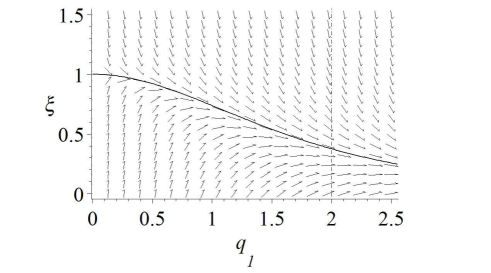
(a)

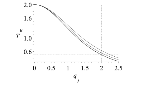
(b)

Figure 1: (a) Direction field corresponding to the Riccati equation (55), where the solution with $\xi(0)=\mu:=\lambda_{2}-\lambda_{1}$, for $\lambda_{2}=2$, $\lambda_{1}=1$, is also plotted. (b) Three solutions of the Riccati equation (55) for $\lambda_{2}=2$: the lowermost one corresponds to $\lambda_{1}=2$ and the other two, in ascending order, to $\lambda_{1}=1.75$ and $\lambda_{1}=1$, respectively. Note that the corresponding to $\lambda_{1}=\lambda_{2}=2$, holds the point $(2,\lambda_{1}/4)=(2,1/2)$.

Using the reversibility.  One sees from Lemma 9 that the Hamiltonian (49) satisfies the reversibility defined in Section 2.5, with respect to the linear involution $\mathcal{R}:(q,p)\mapsto(Rq,-Rp)$, with $R=\mathrm{diag}[r_{1},r_{2}]$, and for any $r_{1},r_{2}=\pm 1$. In particular, if we take $r_{1}=r_{2}=1$, then Proposition 10 yields

$$S_{0}^{{\rm s}}(q_{1})=-S_{0}^{{\rm u}}(q_{1})=-\frac{2\lambda_{1}q_{1}^{\,2}}{4+q_{1}^{\,2}},\quad S_{1}^{{\rm s}}(q_{1})=-S_{1}^{{\rm u}}(q_{1})=0,\quad T^{{\rm s}}(q_{1})=-T^{{\rm u}}(q_{1}).$$ (56)

Let us now consider the other local chart $(\widetilde{\mathcal{U}},\tilde{\varphi}^{*})$. The (local) stable manifolds $\widetilde{\mathcal{W}}^{{\rm s}}$ of the origin $\widetilde{O}:=(\widetilde{q},\widetilde{p})=(0,0)$ (corresponding, in this coordinate system, to the point $\tilde{P}=(0,0,1,0,0,0)$ on the phase space $T^{*}\mathbb{S}^{2}$), can be put as a graph of a function through the same generating function $S^{{\rm s}}$, for the Hamiltonian takes exactly the same expression in both local charts, as we pointed out before. Thus, the manifold $\widetilde{\mathcal{W}}^{{\rm s}}$ is given by $\widetilde{p}=\nabla S^{{\rm s}}(\widetilde{q})$. Therefore, we know from (24) that the change of coordinates (46) yields the identity $\widehat{S}^{{\rm s}}=S^{{\rm s}}\circ\chi+c$, with $c$ constant, and this gives $\widetilde{\mathcal{W}}^{{\rm s}}$ in the coordinates $(q,p)$ of the chart $(\mathcal{U},\varphi)$.

Expanding $\widehat{S}^{{\rm s}}$ around the outgoing part of $\gamma$ given by (52), regarding the reversibility (56) and the components $\chi=(\chi_{1},\chi_{2})$ given in (45), one has

$$\widehat{S}^{{\rm s}}(q) = \widehat{S}^{{\rm s}}_{0}(q_{1})+\widehat{S}^{{\rm s}}_{1}(q_{1})q_{2}+\frac{1}{2}\widehat{T}^{{\rm s}}(q_{1})q_{2}^{\,2}+\cdots$$

$$= c-S^{{\rm u}}_{0}(\chi_{1}(q))-S^{{\rm u}}_{1}(\chi_{1}(q))\chi_{2}(q)-\frac{1}{2}T^{{\rm s}}(\chi_{1}(q))\chi_{2}(q)^{2}+\cdots$$

$$= c-S_{0}^{{\rm u}}\left(\frac{4q_{1}}{q_{1}^{\,2}+q_{2}^{\,2}}\right)-\frac{1}{2}T^{{\rm u}}\left(\frac{4q_{1}}{q_{1}^{\,2}+q_{2}^{\,2}}\right)\frac{16q_{2}^{\,2}}{(q_{1}^{\,2}+q_{2}^{\,2})^{2}}+\cdots$$

$$= c-S_{0}^{{\rm u}}\left(\frac{4}{q_{1}}\right)+\frac{1}{2}\left[\frac{8}{q_{1}^{\,3}}(S^{{\rm u}}_{0})^{\prime}\left(\frac{4}{q_{1}}\right)-\frac{16}{q_{1}^{\,4}}{T}^{{\rm u}}\left(\frac{4}{q_{1}}\right)\right]q_{2}^{\,2}+\cdots,$$

and by comparison of coefficients,

$$\widehat{S}^{{\rm s}}_{0}(q_{1})=c-S^{{\rm u}}_{0}\left(\frac{4}{q_{1}}\right)=c-\frac{8\lambda_{1}}{q_{1}^{\,2}+4},\qquad$$

$$\widehat{T}^{{\rm s}}(q_{1})=\frac{8}{q_{1}^{\,3}}(S^{{\rm u}}_{0})^{\prime}\left(\frac{4}{q_{1}}\right)-\frac{16}{q_{1}^{\,4}}T^{{\rm u}}\left(\frac{4}{q_{1}}\right)=\frac{32\lambda_{1}}{(q_{1}^{\,2}+4)^{2}}-\frac{16}{q_{1}^{\,4}}T^{{\rm u}}\left(\frac{4}{q_{1}}\right)$$

(according to (27), the constant $c$ can be fixed if, for example, we set $\widehat{S}_{0}^{{\rm s}}(2)=S^{{\rm u}}_{0}(2)=\lambda_{1}$; this exacts $c=2\lambda_{1}$). Then, the difference between $T^{{\rm u}}$ and $\widehat{T}^{{\rm s}}$ at $q^{*}_{1}=2$ is

$$T^{{\rm u}}(2)-\widehat{T}^{{\rm s}}(2)=2T^{{\rm u}}(2)-\frac{\lambda_{1}}{2}$$

and therefore,

$$T^{{\rm u}}(2)\neq\frac{\lambda_{1}}{4}$$ (57)

is a necessary and sufficient condition for transversality between $\mathcal{W}^{{\rm u}}$ and $\widetilde{\mathcal{W}}^{{\rm s}}$ along the heteroclinic orbit $\gamma$. This is stated in the proposition below. Notice that, in the chart (44), for $q=(q^{*}_{1},0)=(2,0)$ we obtain the point $(1,0,0)\in\mathbb{S}^{2}$.

Proposition 12

If in the system (43) defined on the $2$-sphere $\mathbb{S}^{2}$, with $A$ the diagonal matrix $A=\mathrm{diag}[\lambda_{1},\lambda_{2},\lambda_{3}]$, we assume $\lambda_{2}>\lambda_{1}>\lambda_{3}=0$; then, for its associated Hamiltonian flow in the phase space $T^{*}\mathbb{S}^{2}$, the stable invariant manifold $\widetilde{\mathcal{W}}^{{\rm s}}$ of the point $\widetilde{\mathcal{P}}=(0,0,1,0,0,0)$ and the unstable invariant manifold $\mathcal{W}^{{\rm u}}$ of the point $\mathcal{P}=(0,0,-1,0,0,0)$ intersect transversely along the orbit $\gamma$ (see (52)).

Proof.  By the considerations in the previous paragraph, it suffices to check the transversality condition (57), which is equivalent to $\xi(2)\neq 0$, where $\xi(q_{1}):=T^{{\rm u}}(q_{1})-T^{\rm u}_{0}(q_{1})$, with $T_{0}^{{\rm u}}(q_{1})$ given by (54); but in the proof of Lemma 11 it is stated that $\xi>0$ for $q_{1}>0$. Thus, in particular, $\xi(2)\neq 0$ is satisfied. This proves the proposition.   

Integrability of the Riccati equation.  Alternatively, the Riccati equation (53) could have been solved explicitly in order to check the transversality condition (57). First, a standard change of type

$$T^{{\rm u}}=\frac{16\lambda_{1}q_{1}}{\left(4+q_{1}^{\,2}\right)^{2}}\cdot\frac{y^{\prime}}{y},$$ (58)

where $T^{{\rm u}}=T^{{\rm u}}(q_{1})$, and $y=y(q_{1})$ is the new unknown function, transforms (53) into the second-order linear equation

$$y^{\prime\prime}-\frac{3q_{1}^{\,2}-4}{q_{1}(4+q_{1}^{\,2})}\,y^{\prime}-\frac{4\lambda_{2}^{\,2}+(\lambda_{2}^{\,2}-4\lambda_{1}^{\,2})q_{1}^{\,2}}{\lambda_{1}^{\,2}q_{1}^{\,2}(4+q_{1}^{\,2})}\,y=0.$$ (59)

Remark.  This is a particular case of the well-known fact that any Riccati equation $z^{\prime\prime}+a(x)z+b(x)z^{2}=c(x)$ transforms into a second-order linear equation, $y^{\prime\prime}+\left(a(x)-\displaystyle\frac{b^{\prime}(x)}{b(x)}\right)y^{\prime}-b(x)c(x)y=0$, through the change $z=\displaystyle\frac{y^{\prime}}{b(x)y}$ .

Now, the Kovacic’s algorithm can be applied to investigate the (Liouvillian) integrability of second-order differential equations with coefficients in the class $\mathbb{C}(x)$ of rational functions (for a complete description of the process and applications, we point the reader to [Kov86], [DL92], [AMW11] and references therein). This algorithm is implemented in some computer algebra systems such as Maple; and when applied to equation (59), it produces the following two fundamental solutions:

$$y_{1}(q_{1})=\left(-4(\lambda_{{2}}+\lambda_{{1}})+(\lambda_{{1}}-\lambda_{{2}})q_{1}^{\,2}\right)q_{1}^{\lambda_{2}/\lambda_{1}},$$

$$y_{2}(q_{1})=\frac{4(\lambda_{{2}}-\lambda_{{1}})+(\lambda_{{1}}+\lambda_{2})q_{1}^{\,2}}{\lambda_{{2}}+\lambda_{1}}\>q_{1}^{-\lambda_{2}/\lambda_{1}};$$

hence, the linear equation (59) is integrable and so it is the Riccati equation (53). Actually, transforming back $y_{1}(q_{1})$ using (58), one obtains a solution of (53),

$$T^{{\rm u}}(q_{1})=\frac{16\lambda_{1}q_{1}}{\left(4+q_{1}^{\,2}\right)^{2}}\cdot\frac{y^{\prime}_{1}(q_{1})}{y_{1}(q_{1})}=\frac{-\left(16\,\lambda_{2}^{\,2}+16\,\lambda_{1}\lambda_{2}\right)\left(q_{1}^{\,2}+4\right)+32\,\lambda_{1}^{\,2}q_{1}^{\,2}}{\left(q_{1}^{\,2}+4\right)^{2}\left(\left(\lambda_{1}-\lambda_{2}\right)q_{1}^{\,2}-4\,\lambda_{1}-4\,\lambda_{2}\right)},$$

with $T^{{\rm u}}(0)=\lambda_{2}$; and since $\lambda_{2}>\lambda_{1}>0$, it is well defined for all $q_{1}>0$. Besides, the transversality condition (57) can also be checked straightforward from this explicit form of the solution of the Riccati equation (53). Indeed, for $q_{1}=2$ it gives

$$T^{{\rm u}}(2)=\frac{1}{4}\left(\lambda_{2}+\lambda_{1}-\frac{\lambda_{1}^{\,2}}{\lambda_{2}}\right)>\frac{\lambda_{1}}{4}$$

for $\lambda_{2}>\lambda_{1}>0$. In Figure 1(b), the function $T^{{\rm u}}$ is plotted for different values of the parameters.

3 The case of a 2-torus: $Q=\mathbb{T}^{2}$

3.1 The generating functions in the periodic case

In what comes, that the configuration space will be the 2-torus, i.e. $Q=\mathbb{T}^{2}=(\mathbb{R}/2\pi\mathbb{Z})^{2}$. In view of the form of the Hamiltonian (1), this is equivalent to suppose that the quadratic form $B(q)$ and the potential $V(q)$ are both $2\pi$-periodic functions with respect to $q=(q_{1},q_{2})$. In this way, the hyperbolic point $O=(0,0,0,0)$ can be identified with $\widetilde{O}=(2\pi,0,0,0)$, and therefore a biasymptotic orbit $\gamma$ connecting both ends is a homoclinic orbit or loop.

Let us introduce coordinates in a neighborhood of $O$ and in a neighborhood of $\widetilde{O}$, denoted $(q,p)=(q_{1},q_{2},p_{1},p_{2})$ and $(\tilde{q},\tilde{p})=(\tilde{q}_{1},\tilde{q}_{2},\tilde{p}_{1},\tilde{p}_{2})$, having the origin at $O$ and $\widetilde{O}$ respectively. It is clear that the change (3) relating them is given by

$$(\tilde{q}_{1},\tilde{q}_{2})=\chi(q_{1},q_{2})=(q_{1}-2\pi,q_{2}),\qquad(\tilde{p}_{1},\tilde{p}_{2})=(p_{1},p_{2}).$$ (60)

since ${\rm D}\chi(q)^{-\top}={\rm Id}$.

Remark.  Due to the periodicity of the Hamiltonian, the corresponding Hamiltonian equations write identically in either coordinates $(q,p)$ or $(\tilde{q},\tilde{p})$. The invariant manifolds $\mathcal{W}^{{\rm u},{\rm s}}$ and $\widetilde{\mathcal{W}}^{{\rm u},{\rm s}}$ are related by the periodicity and, therefore, their generating functions $S^{{\rm u},{\rm s}}$ and $\widetilde{S}^{{\rm u},{\rm s}}$ are the same functions (note however, that the functions $S^{{\rm u},{\rm s}}$ depend on $q$ whilst $\widetilde{S}^{{\rm u},{\rm s}}$ depend on $\tilde{q}$).

We assume the hypotheses (H1–H4) stated in Section 1.1, with some minor modifications in order to adapt them to the case $Q=\mathbb{T}^{2}$ being studied here:

• the orbit $\gamma$ satisfies $q_{2}=0$, with $q_{1}$ increasing along the orbit from $0$ to $2\pi$;

• the generating function $S^{{\rm u}}(q_{1},q_{2})$ of the invariant manifold $\mathcal{W}^{{\rm u}}$ of $O$ is defined in a $\mathbb{R}^{2}$-neighborhood of the segment $0\leq q_{1}\leq\pi$ of type $U=\left(-a,\pi+a\right)\times\left(-\delta,\delta\right)$, for some $a>0$ and $\delta>0$; and conversely, the generating function $\widetilde{S}^{{\rm s}}(\tilde{q}_{1},\tilde{q}_{2})$ of the invariant manifold $\widetilde{W}^{{\rm s}}$ of $\widetilde{O}$ is defined in a $\mathbb{R}^{2}$-neighborhood of the segment $-\pi\leq\tilde{q}_{1}\leq 0$ of type $\widetilde{U}=\left(-\pi-a,a\right)\times\left(-\delta,\delta\right)$.

Applying the change (60), we can write the manifold $\widetilde{W}^{\rm s}$ in the coordinates $(q,p)$. As in (6), it has a generating function, given by $\widehat{S}^{\rm s}=\widetilde{S}^{\rm s}\circ\chi+{\rm const}=S^{\rm s}\circ\chi+\rm const$, that is,

$$\widehat{S}^{\rm s}(q_{1},q_{2})=S^{\rm s}(q_{1}-2\pi,q_{2})+\sigma.$$ (61)

In other words, the generating function $\widehat{S}^{{\rm s}}(q)$ is the function $\widetilde{S}^{{\rm s}}(\tilde{q})$ expressed in the coordinates $q$ and shifted by an additive constant $\sigma$, which will be chosen below.

By hypothesis (H4^′), we see that $S^{\rm u}(q)$ and $\widehat{S}^{\rm s}(q)$ can be compared in their common domain $U\cap\chi^{-1}(\widetilde{U})=\left(\pi-a,\pi+a\right)\times\left(-\delta,\delta\right)$, which is a $\mathbb{R}^{2}$-neighborhood of $q^{*}_{1}=\pi$. As we see below, our choice of this point to check the transversality allows us to take advantage of the reversibility properties of the Hamiltonian.

The generating functions along the loop.  As in the general setting described in Section 2.2, the loop $\gamma$ is described by the coefficients $S_{0}$ and $S_{1}$, of orders 0 and 1, in the expansion in $q_{2}$ of the generating function of any of the invariant manifolds containing it. More precisely, the loop $\gamma$ is given by the equations (26–27), which correspond to the coefficients in the expansions (21) and (25). Such coefficients are, initially, functions of $q_{1}$ defined in a finite interval. Nevertheless, using that they must coincide for the unstable and stable manifolds, together with the $2\pi$-periodicity in $q_{1}$ of the Hamiltonian, we are going to show that such coefficients are $4\pi$-periodic functions of $q_{1}$.

Combining (26–27) with the identity (61), we have

$$\gamma: p_{1}=S^{\prime}_{0}(q_{1}):=(S^{\rm u}_{0})^{\prime}(q_{1})=(\widehat{S}^{\rm s}_{0})^{\prime}(q_{1})=(S^{\rm s}_{0})^{\prime}(q_{1}-2\pi),$$ (62)

$$p_{2}=S_{1}(q_{1}):=S^{\rm u}_{1}(q_{1})=\widehat{S}^{\rm s}_{1}(q_{1})=S^{\rm s}_{1}(q_{1}-2\pi).$$

As a parameterization of $\gamma$, this is valid for $0<q_{1}<2\pi$, but the functions in the equalities can be extended up to a neighborhood of $0\leq q_{1}\leq 2\pi$.

In fact, it is easy to see from the above equations (62) and the reversibility relations of Proposition 10 with $r_{1}=r_{2}=1$ —this is the trivial $\mathcal{R}$-reversibility, see the remark after Lemma 9—, that $S^{\prime}_{0}$ and $S_{1}$ can be extended as $2\pi$-antiperiodic functions:

$$\begin{array}[]{ll}S^{\prime}_{0}(q_{1})=(S^{\rm s}_{0})^{\prime}(q_{1}-2\pi)=-(S^{\rm u}_{0})^{\prime}(q_{1}-2\pi)=-S^{\prime}_{0}(q_{1}-2\pi),\\[4.0pt] S_{1}(q_{1})=S^{\rm s}_{1}(q_{1}-2\pi)=-S^{\rm u}_{1}(q_{1}-2\pi)=-S_{1}(q_{1}-2\pi).\end{array}$$

Thus, the functions $S^{\prime}_{0}(q_{1})$ and $S_{1}(q_{1})$ can be defined for all $q_{1}\in\mathbb{R}$, and are $2\pi$-antiperiodic, and hence they are $4\pi$-periodic and have zero average. It turns out that the coefficient $S_{0}(q_{1})$ (without derivative) is also a $4\pi$-periodic function. Indeed, one can easily check that a primitive of any $2\pi$-antiperiodic function is $4\pi$-periodic.

We point out that this period $4\pi$ is due to the fact that the functions $S^{\prime}_{0}(q_{1})$ and $S_{1}(q_{1})$ parameterize two loops of $O$. Indeed, the loop $\gamma$ is obtained for $0<q_{1}<2\pi$ and satisfies $p_{1}>0$, and another loop is obtained for $2\pi<q_{1}<4\pi$ and satisfies $p_{1}<0$ (see an example in Figures 2(a) and 2(b)).

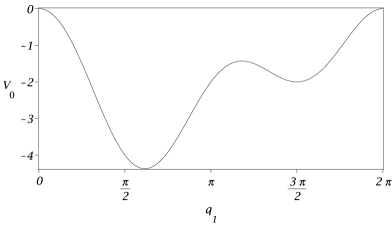
(a)

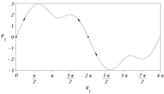
(b)

Figure 2: (a) Graph of the $2\pi$-periodic potential $V_{0}(q_{1})=\cos q_{1}-\sin q_{1}+\cos 2q_{1}-\frac{1}{2}\sin 2q_{1}-2$. (b) Projection onto the plane $(q_{1},p_{1})$ of the loops, given by the graph $p_{1}=S^{\prime}_{0}(q_{1})$ and assuming $\beta(q_{1})=1$ (see Proposition 5(b)); the loop $\gamma$ has $q_{1}$ increasing from $0$ to $2\pi$, and a second loop obtained from the periodicity has $q_{1}$ decreasing from $4\pi$ to $2\pi$.

Now it is clear, by integrating from 0 to $2\pi$ the first equation in (62), that we can write

$$S_{0}(q_{1}):=S^{\rm u}_{0}(q_{1})=\widehat{S}^{\rm s}_{0}(q_{1})=S^{\rm s}_{0}(q_{1}-2\pi)+\sigma,$$

where $\sigma$ is the constant in (61), given by

$$\sigma=\int_{0}^{2\pi}p_{1}\,\mathrm{d}q_{1}=S_{0}(2\pi)-S_{0}(0)=S^{\rm u}_{0}(2\pi)=-S^{\rm s}_{0}(-2\pi),$$ (63)

and we have taken into account our choice $S^{{\rm u},{\rm s}}_{0}(0)=0$ in (21).

The generating functions of the invariant manifolds.  Let us return to the invariant manifolds $\mathcal{W}^{\rm u}$ and $\widetilde{\mathcal{W}}^{\rm s}$, described in the coordinates $(q,p)$ by their generating functions $S^{\rm u}(q_{1},q_{2})$ and $\widehat{S}^{\rm s}(q_{1},q_{2})$. We know from the previous paragraph the relations concerning the coefficients of orders 0 and 1 in their expansions in $q_{2}$, and now we are interested in the coefficients of order 2, which are used in order to study the transversality.

Expanding in $q_{2}$ the identity (61), the coefficients of order 2 satisfy the equality

$$\widehat{T}^{{\rm s}}(q_{1})=T^{{\rm s}}(q_{1}-2\pi).$$

By hypothesis (H4^′), the functions $T^{\rm u}$ and $\widehat{T}^{{\rm s}}$ are defined for $q_{1}\in\left(-a,\pi+a\right)$ and $q_{1}\in\left(\pi-a,2\pi+a\right)$ respectively. Then, they can be compared for $q_{1}\in\left(\pi-a,\pi+a\right)$, which makes a difference with the fact that the coefficients of orders 0 and 1 (giving only the loop in (62)) are functions defined for all $q_{1}\in\mathbb{R}$.

Reversibility relations and transversality.  Finally, we assume the reversibility of the Hamiltonian in the sense stated in Section 2.5, i.e. with respect to an involution $\mathcal{R}$ of the form (40) with the matrix $R=\mathrm{diag}[r_{1},r_{2}]$ given in (41). Since we want to compare $\mathcal{W}^{{\rm u}}$ with $\widetilde{\mathcal{W}}^{{\rm s}}$ along $\gamma$, we shall fix $r_{1}=-1$, for this will be the case of interest: the loop is mapped into itself by the reversibility, $\mathcal{R}\gamma=\gamma$, since it reverses the sign of $q_{1}$, but keeps the sign of $p_{1}$. In other words, for $r_{1}=-1$ the restriction of $\mathcal{R}$ to the plane $(q_{1},p_{1})$ is a symmetry with respect to $q_{1}=0$ (or equivalently $q_{1}=\pi$).

Proposition 13

Under the hypothesis of this section, if the Hamiltonian (1) is $\mathcal{R}$-reversible with $r_{1}=-1$ (and $r_{2}=\pm 1$), then the following equality holds:

$$\widehat{S}^{{\rm s}}(2\pi-q_{1},r_{2}q_{2})=-S^{{\rm u}}(q_{1},q_{2})+\sigma,\qquad(q_{1},q_{2})\in\left(\pi-a,\pi+a\right)\times\left(-\delta,\delta\right),$$ (64)

where $\sigma$ is the constant in (61). Besides, its coefficients satisfy

$$\begin{array}[]{lcll}S_{0}(2\pi-q_{1})&=&-S_{0}(q_{1})+\sigma,&\qquad q_{1}\in\mathbb{R},\\[4.0pt] S_{1}(2\pi-q_{1})&=&-r_{2}S_{1}(q_{1}),&\qquad q_{1}\in\mathbb{R},\\[4.0pt] \widehat{T}^{{\rm s}}(2\pi-q_{1})&=&-T^{{\rm u}}(q_{1}),&\qquad q_{1}\in\left(\pi-a,\pi+a\right).\end{array}$$ (65)

Proof.  We use the reversibility relations given by Proposition 10, with $r_{1}=-1$. The first equality (64) follows from (61) and the first relation in Proposition 10:

$$\widehat{S}^{\rm s}(2\pi-q_{1},r_{2}q_{2})=S^{\rm s}(-q_{1},r_{2}q_{2})+\sigma=-S^{\rm u}(q_{1},q_{2})+\sigma.$$

Expanding this equality in $q_{2}$, we get the remaining three equalities (65).

However, to ensure the validity for $q_{1}\notin\left(\pi-a,\pi+a\right)$ of the first two equalities (65), we should deal with the whole loop. For a given point $(q_{1},0,p_{1},p_{2})\in\gamma$, we have in (62) the equations $p_{1}=S^{\prime}_{0}(q_{1})$ and $p_{2}=S_{1}(q_{1})$. Since $\mathcal{R}$ takes this point into another point of $\gamma$, we also have $p_{1}=S^{\prime}_{0}(2\pi-q_{1})$ and $-r_{2}p_{2}=S_{1}(2\pi-q_{1})$. Then, the functions $S_{0}$ and $S_{1}$ satisfy the identities $S^{\prime}_{0}(2\pi-q_{1})=S^{\prime}_{0}(q_{1})$ and $S_{1}(2\pi-q_{1})=-r_{2}S_{1}(q_{1})$. The second one corresponds to our statement, and integrating the first one we obtain $S_{0}(2\pi-q_{1})=-S_{0}(q_{1})+\rm const$, where for $q_{1}=0$ we see that the constant is $\sigma$, in agreement with (63).   

As a direct consequence of this proposition, we see that in this case $Q=\mathbb{T}^{2}$ the transversality condition (8) becomes very simple. Using the third equality (65) at $q^{*}_{1}=\pi$, we get that the necessary and sufficient condition for the transversality of the invariant manifolds $\mathcal{W}^{\rm u}$ and $\widetilde{\mathcal{W}}^{\rm s}$ along the loop $\gamma$, can be expressed as follows:

$$T^{{\rm u}}(\pi)\neq 0.$$

3.2 Example: two identical connected pendula

As an example with the configuration manifold $Q=\mathbb{T}^{2}$, we consider the system of two identical pendula connected by an interacting potential. This model was considered in [GS95], where the transversality of the invariant manifolds along a loop was established by using the variational equations around it (for other properties of this model, see for instance [Arn89, §23D]). Here, our aim is to apply the method developed in this paper to recover the result of transversality in a somewhat more general model.

Initially, in symplectic coordinates $(\xi,\eta)=(\xi_{1},\xi_{2},\eta_{1},\eta_{2})\in\mathbb{T}^{2}\times\mathbb{R}^{2}$ we consider the Hamiltonian

$$H(\xi,\eta)=\textstyle\frac{1}{2}(\eta_{1}^{\,2}+\eta_{2}^{\,2})+(\cos\xi_{1}-1)+(\cos\xi_{2}-1)+f(\xi_{1})(1-\cos(\xi_{2}-\xi_{1})),$$ (66)

where the interacting term is given by a $2\pi$-periodic even function $f(\xi_{1})$, such that $0\leq f(0)<1/2$. Under this inequality, the origin is a hyperbolic equilibrium point with (different) Lyapunov exponents $\pm 1$, $\pm b$, where we define $b=\sqrt{1-2f(0)}$, $0<b\leq 1$. The case of a constant function $f$, considered in [GS95], corresponds to a linear spring connecting the two pendula. We point out that the term $1-\cos(\xi_{2}-\xi_{1})$ allows us to keep the periodicity in $\xi_{1}$, but could be replaced for instance by $(\xi_{2}-\xi_{1})^{2}/2$.

It is clear that, if we assume $f\equiv 0$ in (66), the system is separable and integrable: it consists of the product of two identical pendula with coordinates $(\xi_{j},\eta_{j})$, $j=1,2$. We have, for each pendulum, the (positive) separatrix

$$\xi_{j}=4\arctan\mathrm{e}^{t},\qquad\eta_{j}=2\sin\frac{\xi_{j}}{2}=\frac{2}{\cosh t}.$$ (67)

Combining the two separatrices, with a free initial condition for one of them, say the first one, we have the following 1-parameter family of loops indexed by $s\in\mathbb{R}$ (see Figure 3(a)),

$$\begin{array}[]{lll}\bar{\gamma}_{s}:&\bar{\xi}_{1}(t,s)=4\arctan\mathrm{e}^{s+t},&\bar{\xi}_{2}(t)=4\arctan\mathrm{e}^{t},\\[2.0pt] &\bar{\eta}_{1}(t,s)=\displaystyle\frac{2}{\cosh(s+t)},&\bar{\eta}_{2}(t)=\displaystyle\frac{2}{\cosh t}.\end{array}$$ (68)

If we consider $f\not\equiv 0$ in (66), in general the family of loops is destroyed, but the concrete loop $\gamma=\bar{\gamma}_{0}$ remains unchanged, as well as the dynamics along it. Our aim is to provide a sufficient condition on the function $f$, ensuring that the invariant manifolds intersect transversely along this loop.

In order to apply the results of Section 2, we perform the symplectic change of coordinates

$$\left(\begin{array}[]{c}\xi_{1}\\[3.0pt] \xi_{2}\end{array}\right)=\varphi(q)=\left(\begin{array}[]{c}q_{1}\\[3.0pt] q_{1}+q_{2}\end{array}\right),\qquad\left(\begin{array}[]{c}\eta_{1}\\[3.0pt] \eta_{2}\end{array}\right)={\rm D}\varphi(q)^{-\top}p=\left(\begin{array}[]{c}p_{1}-p_{2}\\[3.0pt] p_{2}\end{array}\right),$$ (69)

where it is clear that $\xi=\varphi(q)$ is a well-defined change on $\mathbb{T}^{2}$. In the new coordinates $(q,p)$, the expression of the Hamiltonian $H$ takes the form (1), with

$$B(q)=\left(\begin{array}[]{cc}1&-1\\[3.0pt] -1&2\end{array}\right),\quad V(q)=(\cos q_{1}-1)+(\cos(q_{1}+q_{2})-1)+f(q_{1})(1-\cos q_{2}).$$

It is easy to see from Lemma 9 that $H$ is $\mathcal{R}$-reversible, with $r_{1}=r_{2}=-1$ (recall that $f$ is an even function). Now, the loop $\gamma$ lies on the line $q_{2}=0$:

$$q_{1}^{0}(t)=4\arctan\mathrm{e}^{t},\quad q_{2}^{0}(t)=0,\quad p_{1}^{0}(t)=\frac{4}{\cosh t},\quad p_{2}^{0}(t)=\frac{2}{\cosh t}.$$

We know from (26) that the loop is also given by

$$q_{2}=0,\quad p_{1}=S_{0}^{\prime}(q_{1})=4\sin\frac{q_{1}}{2},\quad p_{2}=S_{1}(q_{1})=2\sin\frac{q_{1}}{2}.$$

Notice that these are $4\pi$-periodic functions, in agreement with the considerations of Section 3.1.

Remark.  As an alternative to (69), we might have chosen as $\xi=\varphi(q)$ a rotation taking the line $\xi_{1}=\xi_{2}$ into $q_{2}=0$. This change would lead to a diagonal matrix $B(q)$ and, although it is not a one-to-one change on $\mathbb{T}^{2}$, some arrangements can be done. However, we chose the change (69) since it is a particular case of the change considered for the example of Section 4.2.

Now, we can write down the Riccati equation (36) allowing us to study the transversality. Developing $V(q)$ in $q_{2}$, we get:

$$V_{0}(q_{1})=2(\cos q_{1}-1),\quad V_{1}(q_{1})=-\sin q_{1},\quad Y(q_{1})=\cos q_{1}-f(q_{1}).$$

Then, the Riccati equation for the unstable manifold $\mathcal{W}^{\rm u}$ is

$$2\sin\frac{q_{1}}{2}\,(T^{\rm u})^{\prime}-2\cos\frac{q_{1}}{2}\,T^{\rm u}+2(T^{\rm u})^{2}=-\left(\sin^{2}\frac{q_{1}}{2}+f(q_{1})\right),\qquad T^{\rm u}(0)=\frac{1+b}{2},$$ (70)

where the initial condition comes from Lemma 7. We give below a sufficient condition on $f$, ensuring that the solution of (70) can be extended up to $q_{1}=\pi$, and satisfies the transversality condition $T^{\rm u}(\pi)\neq 0$.

We provide another useful form for the Riccati equation (70) by carrying out the change of variable $x=-\cos(q_{1}/2)$, with a further modification in order to remove the linear term. Writing $T^{\rm u}(q_{1})=(\bar{T}^{\rm u}(x)-x)/2$ and $f(q_{1})=\bar{f}(x)$, we get the equation

$$(1-x^{2})\frac{\mathrm{d}\bar{T}^{\rm u}}{\mathrm{d}x}+(\bar{T}^{\rm u})^{2}=-2(1-x^{2})+(1-2\bar{f}(x)),\qquad\bar{T}^{\rm u}(-1)=b,$$ (71)

and the transversality condition becomes $\bar{T}^{\rm u}(0)\neq 0$.

As in Section 2.6 the Riccati equation (70) can be transformed, through the change $\bar{T}^{\rm u}(x)=\displaystyle\frac{1-x^{2}}{y(x)}\,\displaystyle\frac{\mathrm{d}y}{\mathrm{d}x}$, into the second-order linear differential equation

$$(1-x^{2})\,\frac{\mathrm{d}^{2}y}{\mathrm{d}x^{2}}-2x\frac{\mathrm{d}y}{\mathrm{d}x}+\left(2-\frac{1-2\bar{f}(x)}{1-x^{2}}\right)y=0.$$ (72)

We are going to establish the transversality of the invariant manifolds along the loop $\gamma$ by checking the transversality condition, for a wide class of functions $f$ in (66). We start with the simplest case of a constant function, already considered in [GS95].

Lemma 14

If we consider $1-2\bar{f}(x)\equiv b^{2}$ constant, with $0<b<1$, then the solution of (71) is

$$\bar{T}^{\rm u}_{b}(x)=b-\displaystyle\frac{1-x^{2}}{b-x},$$ (73)

which can be extended up to the interval $x\in\left[-1,b\right)$, and satisfies $\bar{T}^{\rm u}_{b}(0)=b-1/b<0$.

Proof.  In this case, the second-order equation (72) is a generalized Legendre equation, for which a fundamental system of solutions is given by

$$y_{1}(x)=(b+x)\left(\frac{1-x}{1+x}\right)^{b/2},\qquad y_{2}(x)=(b-x)\left(\frac{1+x}{1-x}\right)^{b/2}=y_{1}(-x).$$

We get, from the second one, the solution of (71) as given in (73). This solution obviously satisfies the transversality condition, provided $0<b<1$ (of course, the separable case $b=1$ has to be excluded).   

Proposition 15

If the function $\bar{f}$ satisfies $0<\bar{f}(x)<1/2$ for all $x\in[-1,0]$, then the solution $\bar{T}^{\rm u}(x)$ of (71) can be extended up to the interval $x\in[-1,0]$, and satisfies $\bar{T}^{\rm u}(0)<0$.

Proof.  The argument is similar to the one given for the example of Section 2.6. With a given $\bar{f}(x)$, we write (71) in the normalized form $\displaystyle\frac{\mathrm{d}\bar{T}^{\rm u}}{\mathrm{d}x}=F(x,\bar{T}^{\rm u})$, where the function $F$ is defined for $(x,\bar{T}^{\rm u})\in\left(-1,0\right]\times\mathbb{R}$. Let $c$ and $d$ be positive constants such that $0<c^{2}\leq 1-2\bar{f}(x)\leq d^{2}<1$ for any $x$. Replacing $1-2\bar{f}(x)$ by $c$ and $d$ in (71), we define functions $F_{c}(x,\bar{T}^{\rm u})$ and $F_{d}(x,\bar{T}^{\rm u})$, corresponding to respective differential equations of the type considered in Lemma 14. We know that their associated solutions $\bar{T}_{c}^{\rm u}$ and $\bar{T}_{d}^{\rm u}$ are both defined for $x\in\left[-1,c\right)$ since $c<d$. Combining the initial conditions $\bar{T}_{c}^{\rm u}(-1)=c$, $\bar{T}^{\rm u}(-1)=b$, $\bar{T}_{d}^{\rm u}(-1)=d$, that satisfy $c<b<d$, with the fact that the inequality $F_{c}\leq F\leq F_{d}$ is true for $x>-1$, we see that the solution $\bar{T}^{\rm u}(x)$ is confined between $\bar{T}_{c}^{\rm u}(x)$ and $\bar{T}_{d}^{\rm u}(x)$, and hence it can also be extended up to the whole interval $\left[-1,c\right)$, and satisfies $\bar{T}^{\rm u}(0)<\bar{T}_{d}^{\rm u}(0)<0$.   

Remark.  If the function $f$ in (66) is a trigonometric polynomial, then the change of variable between $q_{1}$ and $x$ leads to a second-order linear differential equation (72), whose coefficients are rational functions of $x$; hence, as in Section 2.6 one can apply Kovacic’s algorithm to see whether (72) is integrable (in the Liouville sense) or not and, when it is, obtain explicit solutions. In such a case, the transversality condition could be checked directly. Nevertheless, applying Proposition 15 we can check the transversality in many cases, even when it is not possible to solve (72) explicitly. As a concrete example, choosing $f(\xi_{1})=(2-\cos\xi_{1})/8$ in (66), we have $\bar{f}(x)=(3-2x^{2})/8$, and applying Kovacic’s algorithm (as implemented in Maple) for this case it turns out that the equation (72) cannot be solved explicitly but, on the other hand, without solving it we see from Proposition 15 that, for this example, the transversality condition is fulfilled.

4 The case of a perturbed Hamiltonian

4.1 Mel^′nikov integrals

Now, we study the invariant manifolds in a Hamiltonian depending on a small perturbation parameter $\varepsilon$,

$$H_{\varepsilon}(q,p)=H(q,p)+\varepsilon H_{*}(q,p).$$ (74)

As in Section 3, we assume that the configuration manifold is $Q=\mathbb{T}^{2}$. For the unperturbed case $\varepsilon=0$, we assume that the Hamiltonian $H_{0}=H$ is in the situation described in Section 3.1. In particular, it has a hyberbolic point $O$ at the origin, with a loop $\gamma$ contained in $q_{2}=0$.

Concerning the invariant manifolds in a neighborhood of the loop, we are going to consider two different situations:

• the unperturbed invariant manifolds $\mathcal{W}^{{\rm u},{\rm s}}$ intersect transversely along the loop $\gamma$;

• the unperturbed invariant manifolds $\mathcal{W}^{{\rm u},{\rm s}}$ coincide along the loop $\gamma$.

We stress that loops of both types (A) and (B) may coexist in the same Hamiltonian $H$ (and each of them can be moved to $q_{2}=0$ by a specific symplectic change), as illustrated by the example of Section 4.2.

Notice that a loop $\gamma$ of type (A) is isolated in the sense that, if an orbit close to $\gamma$ is a loop, it is not contained in a small neighborhood of $\gamma$.

On the other hand, if $\gamma$ is a loop of type (B) it belongs to a $1$-parameter family of loops, filling the 2-dimensional homoclinic manifold or separatrix $\mathcal{W}:=\mathcal{W}^{\rm u}=\mathcal{W}^{\rm s}$.

For $\varepsilon\neq 0$, in both cases (A) and (B) the loop $\gamma$ will not survive in general. Our aim is to study whether, for $\varepsilon$ small enough, there exists a perturbed loop $\gamma_{\varepsilon}$ at distance ${\mathcal{O}}(\varepsilon)$ from $\gamma$, and the perturbed manifolds $\mathcal{W}_{\varepsilon}^{\rm u}$ and $\mathcal{W}_{\varepsilon}^{\rm s}$ intersect transversely along $\gamma_{\varepsilon}$, inside the energy level containing them. We show that, in the case (A), this problem is quite simple and can be solved by applying the implicit function theorem on a transverse section $q_{1}=\rm const$. Instead, in the case (B) we have a problem of splitting of separatrices, which must be re-scaled in order to apply the implicit function theorem, leading to a necessary and sufficient condition which can be expressed in terms of Mel^′nikov integrals. In other words, we have for (A) and (B) a regular and a singular perturbation problem respectively.

It is clear that for $\varepsilon$ small enough we have a perturbed hyperbolic equilibrium point $O_{\varepsilon}$ inherited from $O$, whose invariant manifolds $\mathcal{W}_{\varepsilon}^{{\rm u},{\rm s}}$ can be expressed in terms of perturbed generating functions: $p=\nabla S_{\varepsilon}^{\rm u}(q)$ and $p=\nabla\widehat{S}_{\varepsilon}^{\rm s}(q)$ (see Section 2.2 for the notations). We point out that the identity (61) also applies here to the perturbed case: $\widehat{S}^{\rm s}_{\varepsilon}(q_{1},q_{2})=S^{\rm s}_{\varepsilon}(q_{1}-2\pi,q_{2})+\sigma_{\varepsilon}$.

Let us consider the expansion in $\varepsilon$ of the generating functions,

$$S_{\varepsilon}^{\rm u}(q)=S^{\rm u}(q)+\varepsilon S_{*}^{\rm u}(q)+{\mathcal{O}}(\varepsilon^{2}),\qquad\widehat{S}_{\varepsilon}^{\rm s}(q)=\widehat{S}^{\rm s}(q)+\varepsilon\widehat{S}_{*}^{\rm s}(q)+{\mathcal{O}}(\varepsilon^{2}).$$ (75)

On the other hand, we know from the ideas introduced in Section 2.2 that the transversality of the perturbed manifolds, inside the energy level containing them, can be studied from the expansion in $q_{2}$, up to order 2, of the generating functions (75). For the unstable manifold, we write

$$S_{\varepsilon}^{\rm u}(q)=S_{0,\varepsilon}^{\rm u}(q_{1})+S_{1,\varepsilon}^{\rm u}(q_{1})\,q_{2}+\textstyle\frac{1}{2}T_{\varepsilon}^{\rm u}(q_{1})\,q_{2}^{\,2}+{\mathcal{O}}(q_{2}^{\,3}),$$

with

$$S_{j,\varepsilon}^{\rm u}(q_{1})=S_{j}(q_{1})+\varepsilon S_{j,*}^{\rm u}(q_{1})+{\mathcal{O}}(\varepsilon^{2}),\quad j=0,1,$$

$$T_{\varepsilon}^{\rm u}(q_{1})=T^{\rm u}(q_{1})+\varepsilon T_{*}^{\rm u}(q_{1})+{\mathcal{O}}(\varepsilon^{2}),$$

and analogously for $\widehat{S}_{\varepsilon}^{\rm s}(q)$. Notice that, for $\varepsilon=0$, we have written $S_{j}(q_{1}):=S_{j}^{\rm u}(q_{1})=\widehat{S}_{j}^{\rm s}(q_{1})$, $j=0,1$, since these terms coincide due to the existence of the unperturbed loop $\gamma$ (recall the definitions (27)).

Following a standard terminology (see for instance [DG00]), we define the splitting potential as the difference between the generating functions for the unstable and stable manifolds:

$$\mathcal{L}_{\varepsilon}(q)=\Delta S_{\varepsilon}(q):=S_{\varepsilon}^{\rm u}(q)-\widehat{S}_{\varepsilon}^{\rm s}(q)$$ (76)

(for any functions $f^{\rm u}$ and $\widehat{f}^{\rm s}$, we are using the notation $\Delta f=f^{\rm u}-\widehat{f}^{\rm s}$). We point out that the name ‘splitting potential’ is normally used in the context of splitting of separatrices, i.e. our case (B), but we are considering here a somewhat more general situation. Expanding $\mathcal{L}_{\varepsilon}$ in $q_{2}$, we write

$$\mathcal{L}_{\varepsilon}(q)=\Delta S_{0,\varepsilon}(q_{1})+\Delta S_{1,\varepsilon}(q_{1})\,q_{2}+\textstyle\frac{1}{2}\Delta T_{\varepsilon}(q_{1})\,q_{2}^{\,2}+{\mathcal{O}}(q_{2}^{\,3}).$$

If we consider the expansion $\mathcal{L}_{\varepsilon}=\mathcal{L}+\varepsilon\mathcal{L}_{*}+{\mathcal{O}}(\varepsilon^{2})$, we have

$$\mathcal{L}(q)=\textstyle\frac{1}{2}\Delta T(q_{1})\,q_{2}^{\,2}+{\mathcal{O}}(q_{2}^{\,3}),$$

$$\mathcal{L}_{*}(q)=\Delta S_{0,*}(q_{1})+\Delta S_{1,*}(q_{1})\,q_{2}+\textstyle\frac{1}{2}\Delta T_{*}(q_{1})\,q_{2}^{\,2}+{\mathcal{O}}(q_{2}^{\,3}),$$

where we used that $\Delta S_{0}(q_{1})=\Delta S_{1}(q_{1})=0$, by the existence of the unperturbed loop $\gamma$.

Now, we can rewrite the two hypotheses on the loop, in terms of the unperturbed generating functions. Recalling the transversality condition (8) for the case (A), we have:

• $\Delta T(q_{1})\neq 0$ for any $q_{1}$;

• $\Delta S(q)=0$ for any $q=(q_{1},q_{2})$.

Theorem 16

• If $\gamma$ is a loop of type (A), then for $\varepsilon$ small enough there exists a perturbed loop $\gamma_{\varepsilon}$ biasymptotic to $O_{\varepsilon}$, and the invariant manifolds $\mathcal{W}_{\varepsilon}^{{\rm u},{\rm s}}$ intersect transversely along $\gamma_{\varepsilon}$.

• If $\gamma$ is a loop of type (B) and the conditions

  $$\frac{\partial\mathcal{L}_{*}}{\partial q_{2}}(\pi,0)=\Delta S_{1,*}(\pi)=0,\qquad\frac{\partial^{2}\mathcal{L}_{*}}{\partial q_{2}^{\,2}}(\pi,0)=\Delta T_{*}(\pi)\neq 0$$ (77)

  are fulfilled, then for $\varepsilon\neq 0$ small enough there exists a perturbed loop $\gamma_{\varepsilon}$ biasymptotic to $O_{\varepsilon}$, and the invariant manifolds $\mathcal{W}_{\varepsilon}^{{\rm u},{\rm s}}$ intersect transversely along $\gamma_{\varepsilon}$.

Proof.  As in Section 2.2, the energy level $\mathcal{N}_{\varepsilon}$ containing both perturbed invariant manifolds is given by the equation $H_{\varepsilon}-H_{\varepsilon}(O_{\varepsilon})=0$. Since for $\varepsilon=0$ we have $\frac{\partial H}{\partial p_{1}}=\dot{q}_{1}\neq 0$ on $\gamma$, we see from the implicit function that, near $\gamma$ and for $\varepsilon$ small enough, we can parameterize $\mathcal{N}_{\varepsilon}$ as $p_{1}=g_{\varepsilon}(q_{1},q_{2},p_{2})$. In the coordinates $(q_{1},q_{2},p_{2})$ of $\mathcal{N}_{\varepsilon}$, the intersections between the invariant manifolds $\mathcal{W}_{\varepsilon}^{\rm u}$ and $\mathcal{W}_{\varepsilon}^{\rm s}$ are given by the equation

$$p_{2}=\frac{\partial S_{\varepsilon}^{\rm u}}{\partial q_{2}}(q_{1},q_{2})=\frac{\partial\widehat{S}_{\varepsilon}^{\rm s}}{\partial q_{2}}(q_{1},q_{2}),\qquad\textrm{i.e.}\quad\frac{\partial\mathcal{L}_{\varepsilon}}{\partial q_{2}}(q_{1},q_{2})=0.$$

It is enough to consider the intersections in a transverse section, say $q_{1}=\pi$, and solve the equation for $q_{2}$. Expanding in $q_{2}$, we see that the intersections are given by the solutions of

$$\frac{\partial\mathcal{L}_{\varepsilon}}{\partial q_{2}}(\pi,q_{2})=\Delta S_{1,\varepsilon}(\pi)+\Delta T_{\varepsilon}(\pi)\,q_{2}+{\mathcal{O}}(q_{2}^{\,2})=0.$$ (78)

Now, expanding in $\varepsilon$ and recalling that $\Delta S_{1}=0$, the equation becomes

$$\left(\Delta T(\pi)\,q_{2}+{\mathcal{O}}(q_{2}^{\,2})\right)+\varepsilon\left(\Delta S_{1,*}(\pi)+\Delta T_{*}(\pi)\,q_{2}+{\mathcal{O}}(q_{2}^{\,2})\right)+{\mathcal{O}}(\varepsilon^{2})=0.$$ (79)

Therefore, in the case (A) there is a solution $q_{2}={\mathcal{O}}(\varepsilon)$, and hence the invariant manifolds intersect transversely along a perturbed loop $\gamma_{\varepsilon}$, for $\varepsilon$ small enough.

In the case (B), the fact that $\mathcal{L}(q)=\Delta S(q)=0$ for any $q$ implies that $\displaystyle\frac{\partial\mathcal{L}}{\partial q_{2}}(\pi,q_{2})=\Delta T(\pi)\,q_{2}+{\mathcal{O}}(q_{2}^{\,2})=0$, and hence the expansion (79) begins with terms of order 1 in $\varepsilon$. Then, dividing by $\varepsilon$ the whole equation we obtain:

$$\Delta S_{1,*}(\pi)+\Delta T_{*}(\pi)\,q_{2}+{\mathcal{O}}(q_{2}^{\,2})+{\mathcal{O}}(\varepsilon)=0.$$

Since we assumed in (77) that $\Delta S_{1,*}(\pi)=0$ and $\Delta T_{*}(\pi)\neq 0$, we see that there is a solution $q_{2}={\mathcal{O}}(\varepsilon)$, and hence the invariant manifolds intersect transversely along a perturbed loop $\gamma_{\varepsilon}$, for $\varepsilon\neq 0$ small enough.   

Remark.  In the case (B), it is easy to see from the existence of the perturbed loop $\gamma_{\varepsilon}$ that $\Delta S_{1,*}(q_{1})=0$ for any $q_{1}$. Indeed, parameterizing $\gamma_{\varepsilon}$ by $q_{1}$, we write $q_{2}=f_{\varepsilon}(q_{1})$. It is satisfied that $\displaystyle\frac{\partial\mathcal{L}_{\varepsilon}}{\partial q_{2}}(q_{1},f_{\varepsilon}(q_{1}))=0$. Expanding this equation in $\varepsilon$ and using that for $\varepsilon=0$ we have $\mathcal{L}=0$ and $f(q_{1})=0$, we obtain: $\Delta S_{1,*}(q_{1})=\displaystyle\frac{\partial\mathcal{L}_{*}}{\partial q_{2}}(q_{1},0)=0$.

Remark.  We point out that, for a loop of type (B), it is not enough to impose a condition like (8), and we need as an additional condition that the coefficients $S_{1,*}^{\rm u}(\pi)$ and $\widehat{S}_{1,*}^{\rm s}(\pi)$ coincide. Otherwise, the existence of a perturbed loop $\gamma_{\varepsilon}$ close to $\gamma$ could not be established in general.

The remaining part of this section concerns the case (B), and our aim is to provide an explicit condition allowing us to check (77) in a concrete example. For $\varepsilon=0$, the separatrix $\mathcal{W}$ is a graph $p=\nabla S(q)$, with the generating function $S(q):=S^{\rm u}(q)=\widehat{S}^{\rm s}(q)$, and the inner dynamics on $\mathcal{W}$ is given by the ordinary differential equation

$$\dot{q}=B(q)\nabla S(q).$$ (80)

For a given $q=(q_{1},q_{2})$, denoting $\check{q}(t,q)$ the solution of (80) that satisfies the initial condition $\check{q}(0,q)=q$, we have a loop

$$\check{x}(t,q)=(\check{q}(t,q),\check{p}(t,q)),\qquad\textrm{with \ $\check{p}(t,q)=\nabla S(\check{q}(t,q))$}.$$ (81)

Of course, it will be enough to consider the initial condition in a direction transverse to $q_{2}=0$:

$$q=\kappa(s)=(\kappa_{1}(s),\kappa_{2}(s)),\ \ s\in\left(-a,a\right),\qquad\textrm{with \ $\kappa(0)=(\pi,0)$ \ and \ $\kappa^{\prime}_{2}(0)\neq 0$.}$$ (82)

In this way, we have a 1-parameter family of loops indexed by $s$, that we denote $\bar{\gamma}_{s}$, given by $\bar{q}(t,s):=\check{q}(t,\kappa(s))$. The particular loop contained in $q_{2}=0$ is $\bar{\gamma}_{0}=\gamma$, and we write $q^{0}(t)=(q_{1}^{0}(t),0)=\bar{q}(t,0)$. Notice that $(q_{1},q_{2})=\bar{q}(t,s)$, $(t,s)\in\mathbb{R}\times\left(-a,a\right)$, is a change of parameters for the separatrix $\mathcal{W}$, in a neighborhood of $\gamma$.

As a possible approach, we could see the functions $T_{\varepsilon}^{\rm u}(q_{1})$ and $\widehat{T}_{\varepsilon}^{\rm s}(q_{1})$ as solutions of Riccati equations as in (36), with initial conditions at $q_{1}=0$ and $q_{1}=2\pi$ respectively. Developing such equations in $\varepsilon$ and taking the terms of order 1, the functions $T_{*}^{\rm u}(q_{1})$ and $\widehat{T}_{*}^{\rm s}(q_{1})$ become solutions of linear differential equations, and hence they can be expressed in terms of integrals. Comparing such integrals, one would obtain a condition for the transversality which could be checked.

Nevertheless, similar integrals of Mel^′nikov type can be obtained, in a more direct way, by developing in $\varepsilon$ the Hamilton–Jacobi equation satisfied by the perturbed generating functions (75) and comparing the unstable and stable ones. An analogous approach was previously used in [LMS03] (see also [Sau01]), for the case of invariant manifolds of tori associated to a simple resonance, i.e. with a 1-d.o.f. hyperbolic part. We are going to show that a first order approximation for $\varepsilon$ small of the splitting potential $\mathcal{L}_{\varepsilon}$ defined in (76) is given by the Mel^′nikov potential, defined as the integral

$$L(q)=-\int_{-\infty}^{\infty}\left[H_{*}(\check{x}(t,q))-H_{*}(O)\right]\,\mathrm{d}t,$$ (83)

absolutely convergent due to the fact that $\check{x}(t,q)$ tends to $O$, with exponential bounds, as $t\to\pm\infty$. Essentially, the Mel^′nikov potential is defined as the integral of the perturbation $H_{*}$ on the unperturbed loops. See also [Tre94] for another definition of a Mel^′nikov integral along the loops contained in a separatrix, and [DR97] for the case of a hyperbolic fixed point of a symplectic map.

Theorem 17

The splitting potential is given at first order in $\varepsilon$ by the Mel^′nikov potential: for some constant $c$,

$$\mathcal{L}_{\varepsilon}(q)=\varepsilon(L(q)+c)+{\mathcal{O}}(\varepsilon^{2}).$$

Proof.  Expanding in $\varepsilon$ the generating functions in (76), it is enough to show that the difference of their first order terms is given by the Mel^′nikov potential:

$$S_{*}^{\rm u}(q)-\widehat{S}_{*}^{\rm s}(q)=L(q)+c.$$ (84)

As in the proof of Theorem 6, we use that the perturbed generating functions satisfy the Hamilton–Jacobi equation, but now we expand it in $\varepsilon$. We start with the generating function associated to the unstable manifold: for any $q$, we have

$$H_{\varepsilon}(q,\nabla S^{\rm u}_{\varepsilon}(q))=\mathcal{H}(q)+\varepsilon\mathcal{H}^{\rm u}_{*}(q)+{\mathcal{O}}(\varepsilon^{2})=\varepsilon H_{*}(O)+{\mathcal{O}}(\varepsilon^{2})$$

(to obtain the constant at the right hand side, we expand $H_{\varepsilon}(O_{\varepsilon})$ in $\varepsilon$ and we use that $H(O)=0$ and $\nabla H(O)=0$). The terms of orders 0 and 1 are

$$\mathcal{H}(q)=H(q,\nabla S(q)),$$

$$\mathcal{H}^{\rm u}_{*}(q)=\left\langle\frac{\partial H}{\partial p}(q,\nabla S(q)),\nabla S^{\rm u}_{*}(q)\right\rangle+H_{*}(q,\nabla S(q)).$$

Since for any $q$ we have $\mathcal{H}^{\rm u}_{*}(q)=H_{*}(O)$, we deduce from (1) that $\nabla S^{\rm u}_{*}(q)$ satisfies the following linear partial differential equation:

$$\left\langle B(q)\nabla S(q),\nabla S^{\rm u}_{*}(q)\right\rangle=-[H_{*}(q,\nabla S(q))-H_{*}(O)].$$ (85)

In the solution of this equation, the characteristic curves play an essential rôle. Since they are given by the ordinary differential equation (80), the characteristic curves are projections of the unperturbed loops (81) onto the configuration space: $q=\check{q}(t,q)$.

What follows is a standard argument for the Poincaré–Mel^′nikov method. Using that $S^{\rm u}_{*}(\check{q}(t,q))$ tends to $S^{\rm u}_{*}(0,0)$ as $t\to-\infty$ for any $q$, we see that

$$S^{\rm u}_{*}(q)-S^{\rm u}_{*}(0,0)=\int_{-\infty}^{0}\frac{\mathrm{d}}{\mathrm{d}t}\left[S^{\rm u}_{*}(\check{q}(t,q))\right]\,\mathrm{d}t=\int_{-\infty}^{0}\left\langle\nabla S^{\rm u}_{*}(\check{q}(t,q)),\dot{\check{q}}(t,q)\right\rangle\,\mathrm{d}t$$

$$\phantom{S^{\rm u}_{*}(q)-S^{\rm u}_{*}(0)}=-\int_{-\infty}^{0}[H_{*}(\check{x}(t,q))-H_{*}(O)]\,\mathrm{d}t,$$

where we have used (80) together with (85). Proceeding analogously with the generating function associated to the stable manifold, we have

$$\widehat{S}^{\rm s}_{*}(2\pi,0)-\widehat{S}^{\rm s}_{*}(q)=-\int_{0}^{\infty}[H_{*}(\check{x}(t,q))-H_{*}(O)]\,\mathrm{d}t,$$

and adding the two expressions we get the identity (84), with $c=S^{\rm u}_{*}(0,0)-\widehat{S}^{\rm s}_{*}(2\pi,0)$.   

We see from this result that, in terms of the Mel^′nikov potential, the transversality condition (77) becomes

$$\frac{\partial L}{\partial q_{2}}(\pi,0)=\Delta S_{1,*}(\pi)=0,\qquad\frac{\partial^{2}L}{\partial q_{2}^{\,2}}(\pi,0)=\Delta T_{*}(\pi)\neq 0.$$ (86)

Now, we show in the following easy lemma that the Mel^′nikov potential $L$ is constant along each loop or, in other words, it is a first integral of the inner dynamics on the separatrix, given by (80).

Lemma 18

The value of $L(\check{q}(\tau,q))$ does not depend on $\tau$.

Proof.  It is enough to carry out the change of variable $t\mapsto t-\tau$ in the integral (83), together with using the identity $\check{x}(t,\check{q}(\tau,q))=\check{x}(t+\tau,q)$.   

As a consequence, the splitting potential can be studied in terms of the parameter $s$ introduced in (82). With this in mind, and denoting $\bar{x}(t,s):=\check{x}(t,\kappa(s))$, we define the reduced Mel^′nikov potential as

$$\widetilde{L}(s):=L(\kappa(s))=-\int_{-\infty}^{\infty}\left[H_{*}(\bar{x}(t,s))-H_{*}(O)\right]\,\mathrm{d}t,\quad s\in\left(-a,a\right).$$ (87)

We show in the next result that the transversality condition can also be written in terms of $\widetilde{L}(s)$ (for an illustration, see the example of Section 4.2).

Proposition 19

If the reduced Mel^′nikov potential $\widetilde{L}(s)$ has a nondegenerate critical point at $s=0$, then for $\varepsilon\neq 0$ small enough there exists a perturbed loop $\gamma_{\varepsilon}$ biasymptotic to $O_{\varepsilon}$, and the invariant manifolds $\mathcal{W}_{\varepsilon}^{{\rm u},{\rm s}}$ intersect transversely along $\gamma_{\varepsilon}$.

Proof.  We first show that

$$\widetilde{L}^{\prime}(0)=0\qquad\Longleftrightarrow\qquad\frac{\partial L}{\partial q_{2}}(\pi,0)=0$$

and, when this is satisfied, we also show that

$$\widetilde{L}^{\prime\prime}(0)\neq 0\qquad\Longleftrightarrow\qquad\frac{\partial^{2}L}{\partial q_{2}^{\,2}}(\pi,0)\neq 0.$$

Then, the transversality condition (86) is fulfilled when the reduced potential $\widetilde{L}(s)$ has a nondegenerate critical point at $s=0$.

To show the two equivalences, we use the identity

$$L(\bar{q}(t,s))=\widetilde{L}(s),$$ (88)

which comes from Lemma 18 and the fact that $\bar{q}(0,s)=\kappa(s)$. The first derivative with respect to $s$ of the identity (88) provides

$$\frac{\partial L}{\partial q_{1}}(\bar{q}(t,s))\,\frac{\partial\bar{q}_{1}}{\partial s}(t,s)+\frac{\partial L}{\partial q_{2}}(\bar{q}(t,s))\,\frac{\partial\bar{q}_{2}}{\partial s}(t,s)=\widetilde{L}^{\prime}(s),$$

Considering $s=0$ and using that $L$ is constant along $q_{2}=0$, we get the equality $\displaystyle\frac{\partial L}{\partial q_{2}}(\bar{q}(t,0))\,\frac{\partial\bar{q}_{2}}{\partial s}(t,0)=\widetilde{L}^{\prime}(0)$. Since by (82) we have $\displaystyle\frac{\partial\bar{q}_{2}}{\partial s}(0,0)=\kappa^{\prime}_{2}(0)\neq 0$, we obtain the first equivalence. Now, assuming that $\widetilde{L}^{\prime}(0)=0$ we deduce that $\displaystyle\frac{\partial L}{\partial q_{2}}(\bar{q}(t,0))=0$ at least in a neighborhood of $t=0$. Thus, we have $\displaystyle\frac{\partial^{2}L}{\partial q_{1}^{\,2}}(\pi,0)=\frac{\partial^{2}L}{\partial q_{1}\,\partial q_{2}}(\pi,0)=0$, and hence the second derivative with respect to $s$ of (88), at $s=t=0$, provides

$$\frac{\partial^{2}L}{\partial q_{2}^{\,2}}(\pi,0)\,\kappa^{\prime}_{2}(0)^{2}=\widetilde{L}^{\prime\prime}(0),$$

which implies the second equivalence.   

Remark.  If one defines the splitting function as $\mathcal{M}_{\varepsilon}(q)=\displaystyle\frac{\partial\mathcal{L}_{\varepsilon}}{\partial q_{2}}(q)$, this provides a measure of the distance between the invariant manifolds in the $p_{2}$-direction. At first order, this function can be approximated in terms of the Mel^′nikov function $M(q)=\displaystyle\frac{\partial L}{\partial q_{2}}(q)$, or the reduced one $\widetilde{M}(s)=\widetilde{L}^{\prime}(s)$, which has to have a simple zero at $s=0$, as the condition for the transversality of the invariant manifolds.

To end this section, we revisit the above results assuming for the perturbed Hamiltonian a suitable type of reversibility (see Section 2.5).

Proposition 20

If the Hamiltonian $H_{\varepsilon}$ is $\mathcal{R}$-reversible with $r_{1}=r_{2}=-1$, then $\mathcal{L}_{\varepsilon}(\pi,q_{2})$ and $L(\pi,q_{2})$ are even functions in $q_{2}$.

Proof.  We see from the considerations of Section 3.1, in particular Proposition 13, that the generating functions of the invariant manifolds $\mathcal{W}^{{\rm u},{\rm s}}_{\varepsilon}$ are related by $\widehat{S}^{\rm s}_{\varepsilon}(2\pi-q_{1},-q_{2})=-S^{\rm u}_{\varepsilon}(q_{1},q_{2})+\sigma_{\varepsilon}$. Then, we obtain

$$\mathcal{L}_{\varepsilon}(\pi,q_{2})=S^{\rm u}_{\varepsilon}(\pi,q_{2})+S^{\rm u}_{\varepsilon}(\pi,-q_{2})+\sigma_{\varepsilon},$$

an even function. This applies also to the Mel^′nikov potential $L(\pi,q_{2})$, though one could also check that this is an even function directly from its definition (83).   

Clearly, the fact that $\mathcal{L}_{\varepsilon}(\pi,q_{2})$ is even in $q_{2}$ implies that the equation (78) always has $q_{2}=0$ as a solution, implying the existence of a perturbed loop $\gamma_{\varepsilon}$ (whose $q_{2}$-coordinate coincides with $\gamma$ at $q_{1}=\pi$ but, in general, we will have $\gamma_{\varepsilon}\neq\gamma$). Nevertheless, an additional condition has to be imposed in order to ensure the transversality of the invariant manifolds along the loop $\gamma_{\varepsilon}$.

Additionally, if we choose $q=\kappa(s)$ in (82) in such a way that the family of unperturbed loops satisfies $\bar{\gamma}_{-s}=\mathcal{R}\bar{\gamma}_{s}$, then the reduced Mel^′nikov potential $\widetilde{L}(s)$ is an even function in $s$. Then, it always has a critical point at $s=0$, and we only have to check its nondegeneracy, $\widetilde{L}^{\prime\prime}(0)\neq 0$, in order to ensure transversality.

4.2 Example: two different weakly connected pendula

In symplectic coordinates $(\xi,\eta)\in\mathbb{T}^{2}\times\mathbb{R}^{2}$ we consider the Hamiltonian

$$H_{\varepsilon}(\xi,\eta)=\textstyle\frac{1}{2}(\eta_{1}^{\,2}+\eta_{2}^{\,2})+(\cos\xi_{1}-1)+\lambda^{2}(\cos\xi_{2}-1)+\varepsilon(1-\cos(\xi_{2}-\xi_{1})),$$

where $\varepsilon$ is a small parameter, and $\lambda\geq 1$ is a fixed value (recall that the case $\lambda=1$ has already been considered in Section 3.2).

For $\varepsilon=0$ the system is separable, and consists of two pendula with Lyapunov exponents $\pm 1$ and $\pm\lambda$, generalizing the separable case of Section 3.2. On the region $\eta_{1},\eta_{2}\geq 0$ (the other three ones are symmetric), it has a 1-parameter family of loops $\bar{\gamma}_{s}$, $s\in\mathbb{R}$, plus two special loops $\widehat{\gamma}_{1}$ and $\widehat{\gamma}_{2}$ with a different topological behavior. The two special loops are given by the separatrix of first/second pendulum, with the equilibrium point of the second/first pendulum:

$$\widehat{\gamma}_{1}:\qquad\xi_{1}(t)=4\arctan\mathrm{e}^{t},\quad\eta_{1}(t)=\displaystyle\frac{2}{\cosh t}\,,\quad\xi_{2}(t)=\eta_{2}(t)=0,$$

$$\widehat{\gamma}_{2}:\qquad\xi_{1}(t)=\eta_{1}(t)=0,\quad\xi_{2}(t)=4\arctan\mathrm{e}^{\lambda t},\quad\eta_{2}(t)=\displaystyle\frac{2\lambda}{\cosh\lambda t}\,;$$

and the 1-parameter family is given by the separatrices of the two pendula, with a free initial condition in one of them (see Figure 3(b)):

$$\begin{array}[]{lll}\bar{\gamma}_{s}:&\bar{\xi}_{1}=\bar{\xi}_{1}(t,s)=4\arctan\mathrm{e}^{t-s},&\bar{\xi}_{2}=\bar{\xi}_{2}(t)=4\arctan\mathrm{e}^{\lambda t},\\[4.0pt] &\bar{\eta}_{1}=\bar{\eta}_{1}(t,s)=\displaystyle\frac{2}{\cosh(t-s)}\,,&\bar{\eta}_{2}=\bar{\eta}_{2}(t)=\displaystyle\frac{2\lambda}{\cosh\lambda t}\,.\end{array}$$

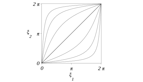
(a)

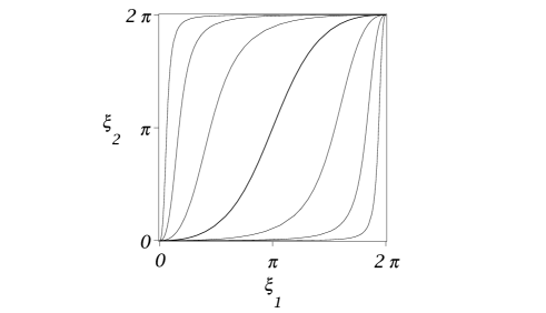
(b)

Figure 3: The 1-parameter family of loops in the separable case,  (a) for $\lambda=1$;  (b) for $\lambda=2.5$.

It is not hard to see that the loops $\widehat{\gamma}_{1}$ and $\widehat{\gamma}_{2}$ are of type (A). Indeed, the unperturbed unstable/stable invariant manifolds of the loop $\widehat{\gamma}_{1}$ are given by the separatrix of the first pendulum, times the local unstable/stable curves of the equilibrium point of the second pendulum: recalling (67), their equations are $\eta_{1}=2\sin(\xi_{1}/2)$, $\eta_{2}=\pm 2\lambda\sin(\xi_{2}/2)$ (with the signs $+$/$-$ for the unstable/stable manifold respectively), and it is clear that they intersect transversely. Then, we see as a consequence of Theorem 16(a) that the equilibrium point $O_{\varepsilon}=O$ has a perturbed loop $\widehat{\gamma}_{1,\varepsilon}$ whose invariant manifolds intersect transversely along it for $\varepsilon$ small enough (from the Hamiltonian equations, one sees that for $\varepsilon\neq 0$ there is no orbit contained in $\xi_{2}=0$, and hence $\widehat{\gamma}_{1,\varepsilon}\neq\widehat{\gamma}_{1}$). The same considerations are valid for the loop $\widehat{\gamma}_{2}$, since we did not use the fact that $\lambda\geq 1$, and both loops are completely analogous.

Now, we study the loop $\gamma=\bar{\gamma}_{0}$, corrsponding to $s=0$ in the 1-parameter family. The existence of this family implies that this is a loop of type (B), whose separatrix $\mathcal{W}$ is the manifold defined by the equations $\eta_{1}=2\sin(\xi_{1}/2)$, $\eta_{2}=2\lambda\sin(\xi_{2}/2)$, $0<\xi_{1},\xi_{2}<2\pi$. The manifold $\mathcal{W}$ contains the whole family of loops $\bar{\gamma}_{s}$, $s\in\mathbb{R}$.

In order to introduce new coordinates $(q,p)$ such that the loop $\gamma$ is contained in $q_{2}=0$, we take into account that the $\xi$-projection of the loop $\gamma$ is the graph

$$\xi_{2}=h(\xi_{1}):=4\arctan\left(\tan^{\lambda}\frac{\xi_{1}}{4}\right).$$

This function $h:\mathbb{T}\rightarrow\mathbb{T}$ is of class $\mathcal{C}^{r}$, where $r$ is the integer part of $\lambda$, and $h$ is analytic if $\lambda$ is integer. Notice that we can consider $h$ as an odd function, since the equality $h(2\pi-\xi_{1})=2\pi-h(\xi_{1})$ is fulfilled.

Thus, we consider the change of coordinates

$$\left(\begin{array}[]{c}\xi_{1}\\[3.0pt] \xi_{2}\end{array}\right)=\varphi(q)=\left(\begin{array}[]{c}q_{1}\\[3.0pt] h(q_{1})+q_{2}\end{array}\right),$$

$$\left(\begin{array}[]{c}\eta_{1}\\[3.0pt] \eta_{2}\end{array}\right)={\rm D}\varphi(q)^{-\top}p=\left(\begin{array}[]{cc}1&-h^{\prime}(q_{1})\\[3.0pt] 0&1\end{array}\right)\left(\begin{array}[]{c}p_{1}\\[3.0pt] p_{2}\end{array}\right).$$

(notice that $x=\varphi(q)$ is a well-defined change on $\mathbb{T}^{2}$). In the new coordinates $(q,p)$ the Hamiltonian takes the form (74) where, for the unperturbed part $H$, we have

$$B(q)=\left(\begin{array}[]{cc}1&-h^{\prime}(q_{1})\\[3.0pt] -h^{\prime}(q_{1})&1+h^{\prime}(q_{1})^{2}\end{array}\right),$$ (93)

$$V(q)=(\cos q_{1}-1)+\lambda^{2}(\cos(h(q_{1})+q_{2})-1),$$ (94)

and the perturbation $\varepsilon H_{*}$ is given by

$$H_{*}(q)=1-\cos(h(q_{1})-q_{1}+q_{2}).$$ (95)

Let us write down, for $\varepsilon=0$, the $q$-coordinates of the unperturbed loops,

$$\bar{\gamma}_{s}:\quad\bar{q}_{1}=\bar{\xi}_{1}=4\arctan\mathrm{e}^{t-s},\quad\bar{q}_{2}=\bar{\xi}_{2}-h(\bar{\xi}_{1})=4\arctan\mathrm{e}^{\lambda t}-4\arctan\mathrm{e}^{\lambda(t-s)},$$ (96)

and it is clear that the loop $\gamma=\bar{\gamma}_{0}$ is now contained in $q_{2}=0$. As in (82), the initial conditions in (96) are given by $\kappa(s)=(4\arctan\mathrm{e}^{-s},\pi-4\arctan\mathrm{e}^{-\lambda s})$, a direction transverse to $q_{2}=0$ for $s=0$.

As we easily check, the perturbed Hamiltonian $H_{\varepsilon}$ in (93–95) is $\mathcal{R}$-reversible with $r_{1}=r_{2}=-1$ (using that the functions $h$ and $h^{\prime}$ are odd and even respectively). Then, we see from Proposition 20 that there exists a perturbed loop $\gamma_{\varepsilon}$ close to $\gamma$.

To study the transversality of the perturbed invariant manifolds along $\gamma_{\varepsilon}$, we use the reduced Mel^′nikov potential:

$$\widetilde{L}(s) = -\int_{-\infty}^{\infty}H_{*}(\bar{q})\,\mathrm{d}t=-\int_{-\infty}^{\infty}\left[1-\cos(h(\bar{q}_{1})-\bar{q}_{1}+\bar{q}_{2})\right]\,\mathrm{d}t$$ (97)

$$= -\int_{-\infty}^{\infty}\left[1-\cos(\bar{\xi}_{2}-\bar{\xi}_{1})\right]\,\mathrm{d}t,$$

where the expressions for $\bar{\xi}_{1}=\bar{\xi}_{1}(t,s)$ and $\bar{\xi}_{2}=\bar{\xi}_{2}(t)$ have been introduced in (68).

The following result implies, according to Proposition 19, that the invariant manifolds intersect transversely along the perturbed loop $\gamma_{\varepsilon}$ for $\varepsilon\neq 0$ small enough, at least for the interval of $\lambda$ considered.

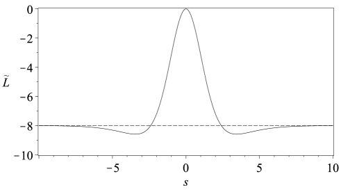
Figure 4: The reduced Mel^′nikov potential $\widetilde{L}(s)$ for $\lambda=1$.

Proposition 21

Assuming that $1\leq\lambda\leq\lambda_{0}\simeq 3.68078$, the reduced Mel^′nikov potential (97) has a nondegenerate critical point at $s=0$.

Proof.  Differentiating (97) with respect to $s$, we obtain:

$$\begin{array}[]{l}\displaystyle\widetilde{L}^{\prime}(s)=\int_{-\infty}^{\infty}\sin(\bar{\xi}_{2}-\bar{\xi}_{1})\,\frac{\partial\bar{\xi}_{1}}{\partial s}\,\mathrm{d}t,\\ \displaystyle\widetilde{L}^{\prime\prime}(s)=-\int_{-\infty}^{\infty}\left[\cos(\bar{\xi}_{2}-\bar{\xi}_{1})\,\left(\frac{\partial\bar{\xi}_{1}}{\partial s}\right)^{2}-\sin(\bar{\xi}_{2}-\bar{\xi}_{1})\,\frac{\partial^{2}\bar{\xi}_{1}}{\partial s^{\,2}}\right]\,\mathrm{d}t,\end{array}$$ (98)

where we have $\displaystyle\frac{\partial\bar{\xi}_{1}}{\partial s}=-2\sin(\bar{\xi}_{1}/2)$ and $\displaystyle\frac{\partial^{2}\bar{\xi}_{1}}{\partial s^{\,2}}=\sin\bar{\xi}_{1}$.

Due to the $\mathcal{R}$-reversibility and the fact that the family of unperturbed loops satisfies $\bar{\gamma}_{-s}=\mathcal{R}\bar{\gamma}_{s}$, it turns out that $\widetilde{L}(s)$ is an even function, and hence $\widetilde{L}^{\prime}(0)=0$ (this is a consequence of Proposition 20, or may also be checked directly).

Now, let us see that $L^{\prime\prime}(0)<0$, at least for a large interval of values of the parameter $\lambda$. We are going to show that for $s=0$ the function inside the integral in (98),

$$f(t)=4\cos(\bar{\xi}_{2}-\bar{\xi}_{1})\,\sin^{2}\frac{\bar{\xi}_{1}}{2}-\sin(\bar{\xi}_{2}-\bar{\xi}_{1})\,\sin\bar{\xi}_{1},$$

is positive for any $t\in\mathbb{R}$. Notice that for $s=0$ we have $\bar{\xi}_{1}=4\arctan\mathrm{e}^{t}$ and $\bar{\xi}_{2}=h(\bar{\xi}_{1})=4\arctan\mathrm{e}^{\lambda t}$.

For any $t>0$, the difference $\bar{\xi}_{2}-\bar{\xi}_{1}$ is positive, and reaches its maximum value $\Xi_{\lambda}$ when $t$ is such that $\cosh\lambda t=\lambda\cosh t$. Using that $\bar{\xi}_{2}=h(\bar{\xi}_{1})$ is increasing in $\lambda$ for $t>0$, then we see that $\Xi_{\lambda}$ is also increasing from 0 to $\pi$ as $\lambda$ goes from 1 to $\infty$. Therefore, there exists a value $\lambda_{0}$ such that $\Xi_{\lambda_{0}}=\pi/2$, and numerically we see that $\lambda_{0}\simeq 3.68078$.

If $1\leq\lambda\leq\lambda_{0}$, then for $t>0$ we have $\pi<\bar{\xi}_{1}<2\pi$ and $0\leq\bar{\xi}_{2}-\bar{\xi}_{1}\leq\pi/2$, and this implies that $f(t)\geq 0$ for any $t>0$. Similar inequalities show that $f(t)\geq 0$ for $t<0$, and we also have $f(0)=4$.   

Remark.  Of course, it is not necessary to have a function $f(t)$ positive for all $t$, in order to obtain a positive integral. Numerically, one can see that the result of Proposition 21 is valid for other values of $\lambda$, larger than $\lambda_{0}$.

Finally we point out, for integer values of $\lambda$, the Mel^′nikov potential (97) could be computed explicitly by writing it as the integral of a rational function. Applying standard trigonometric and hyperbolic formulas, and replacing $t\to\frac{s}{2}+t$, the integral becomes

$$\widetilde{L}(s)=-2\int_{-\infty}^{\infty}\left[\frac{\sinh\left(\frac{s}{2}-t\right)+\sinh\lambda\left(\frac{s}{2}+t\right)}{\cosh\left(\frac{s}{2}-t\right)\cdot\cosh\lambda\left(\frac{s}{2}+t\right)}\right]^{2}\,\mathrm{d}t.$$

This can be transformed into the integral of a rational function, if $\lambda$ is integer, through the change $x=\tanh t$. This change is analogous to the one carried out in Section 3.2, transforming the Riccati equation (70) into an equation with rational coefficients (in fact, the change $x=\tanh t$ is the composition of $q_{1}=4\arctan\mathrm{e}^{t}$ and $x=-\cos(q_{1}/2)$).

For instance, in the simplest case $\lambda=1$ we obtain

$$\widetilde{L}(s) = -8\sinh^{2}{\textstyle\frac{s}{2}}\cdot\int_{-1}^{1}\frac{\mathrm{d}x}{\left(\cosh^{2}\frac{s}{2}-x^{2}\sinh^{2}\frac{s}{2}\right)^{2}}$$

$$= -4\tanh{\textstyle\frac{s}{2}}\cdot\left(\frac{s}{\cosh^{2}\frac{s}{2}}+2\tanh\textstyle\frac{s}{2}\right).$$

A numerical inspection of this function (see Figure 4) shows that it has 2 additional critical points, associated for $\varepsilon\neq 0$ small enough to other perturbed loops.

Acknowledgments.  We would like to express our sincere thanks to Sergey V. Bolotin for his indications about the existence of homoclinic orbits, and to Primitivo Acosta-Humánez and J. Tomás Lázaro for useful discussions and remarks about Riccati equations and the Kovacic’s algorithm.

References

- [AMW11] P.B. Acosta-Humánez, J.J. Morales-Ruiz, and J.-A. Weil. Galoisian approach to integrability of Schrödinger equation. Rep. Math. Phys., 67(3):305–374, 2011.
- [Arn64] V.I. Arnol′d. Instability of dynamical systems with several degrees of freedom. Soviet Math. Dokl., 5(3):581–585, 1964.
- [Arn89] V.I. Arnol′d. Mathematical methods of classical mechanics, volume 60 of Grad. Texts in Math. Springer-Verlag, New York, 2nd edition, 1989.
- [BG86] G. Benettin and G. Gallavotti. Stability of motions near resonances in quasi-integrable Hamiltonian systems. J. Statist. Phys., 44(3-4):293–338, 1986.
- [Bol78] S.V. Bolotin. Libration motions of natural dynamical systems (in Russian). Vestnik Moskov. Univ. Ser. I Mat. Mekh., (1978:6):72–77, 1978.
- [BR98a] S.V. Bolotin and P.H. Rabinowitz. A variational construction of chaotic trajectories for a Hamiltonian system on a torus. Boll. Unione Mat. Ital. Sez. B Artic. Ric. Mat. (8), 1(3):541–570, 1998.
- [BR98b] S.V. Bolotin and P.H. Rabinowitz. A variational construction of chaotic trajectories for a reversible Hamiltonian system. J. Differential Equations, 148(2):364–387, 1998.
- [CL55] E.A. Coddington and N. Levinson. Theory of ordinary differential equations. McGraw-Hill, New York–Toronto–London, 1955.
- [Dev78] R.L. Devaney. Transversal homoclinic orbits in an integrable system. Amer. J. Math., 100(3):631–642, 1978.
- [DG00] A. Delshams and P. Gutiérrez. Splitting potential and the Poincaré–Melnikov method for whiskered tori in Hamiltonian systems. J. Nonlinear Sci., 10(4):433–476, 2000.
- [DG01] A. Delshams and P. Gutiérrez. Homoclinic orbits to invariant tori in Hamiltonian systems. In C.K.R.T. Jones and A.I. Khibnik, editors, Multiple-Time-Scale Dynamical Systems (Minneapolis, MN, 1997), volume 122 of IMA Vol. Math. Appl., pages 1–27. Springer-Verlag, New York, 2001.
- [DG04] A. Delshams and P. Gutiérrez. Exponentially small splitting for whiskered tori in Hamiltonian systems: continuation of transverse homoclinic orbits. Discrete Contin. Dyn. Syst., 11(4):757–783, 2004.
- [DGKP10] A. Delshams, P. Gutiérrez, O. Koltsova, and J.R. Pacha. Transverse intersections between invariant manifolds of doubly hyperbolic invariant tori, via the Poincaré–Mel′nikov method. Regul. Chaotic Dyn., 15(2-3):222–236, 2010.
- [DL92] A. Duval and M. Loday-Richaud. Kovačič’s algorithm and its application to some families of special functions. Appl. Algebra Engrg. Comm. Comput., 3(3):211–246, 1992.
- [DR97] A. Delshams and R. Ramírez-Ros. Melnikov potential for exact symplectic maps. Comm. Math. Phys., 190:213–245, 1997.
- [Eli94] L.H. Eliasson. Biasymptotic solutions of perturbed integrable Hamiltonian systems. Bol. Soc. Brasil. Mat. (N.S.), 25(1):57–76, 1994.
- [GS95] V.G. Gelfreich and D.K. Sharomov. Examples of Hamiltonian systems with transversal homoclinic orbits. Phys. Lett. A, 197(2):139–146, 1995.
- [Hal95] G. Haller. Diffusion at intersecting resonances in Hamiltonian systems. Phys. Lett. A, 200(1):34–42, 1995.
- [Hal97] G. Haller. Universal homoclinic bifurcations and chaos near double resonances. J. Statist. Phys., 86(5-6):1011–1051, 1997.
- [KLDG05] O. Koltsova, L.M. Lerman, A. Delshams, and P. Gutiérrez. Homoclinic orbits to invariant tori near a homoclinic orbit to center–center–saddle equilibrium. Phys. D, 201(3-4):268–290, 2005.
- [Kov86] J.J. Kovacic. An algorithm for solving second order linear homogeneous differential equations. J. Symbolic Comput., 2(1):3–43, 1986.
- [LMS03] P. Lochak, J.-P. Marco, and D. Sauzin. On the splitting of invariant manifolds in multidimensional near-integrable Hamiltonian systems. Mem. Amer. Math. Soc., 163(775), 2003.
- [Mos80] J. Moser. Various aspects of integrable Hamiltonian systems. In Dynamical systems (C.I.M.E. Summer School, Bressanone, 1978), volume 8 of Progr. Math., pages 233–289. Birkhäuser Boston, Mass., 1980.
- [Nek77] N.N. Nekhoroshev. An exponential estimate of the time of stability of nearly-integrable Hamiltonian systems. Russian Math. Surveys, 32(6):1–65, 1977. (Uspekhi Mat. Nauk, 32(6):5–66, 1977).
- [RT06] M. Rudnev and V. Ten. A model for separatrix splitting near multiple resonances. Regul. Chaotic Dyn., 11(1):83–102, 2006.
- [Sau01] D. Sauzin. A new method for measuring the splitting of invariant manifolds. Ann. Sci. École Norm. Sup. (4), 34(2):159–221, 2001.
- [Tre94] D.V. Treschev. Hyperbolic tori and asymptotic surfaces in Hamiltonian systems. Russian J. Math. Phys., 2(1):93–110, 1994.