1. Introduction

The premise of the paper is that it is much easier to solve a boundary integral equation (BIE) defined on a curve in $\mathbb{R}^{2}$ than one defined on a surface in $\mathbb{R}^{3}$. With the development of high order accurate Nyström discretization techniques [14, 2, 15, 5, 13], it has become possible to attain close to double precision accuracy in 2D using only a very moderate number of degrees of freedom. This opens up the possibility of solving a BIE on a rotationally symmetric surface with the same efficiency since such an equation can in principle be written as a sequence of BIEs defined on a generating curve. However, there is a practical obstacle: The kernels in the BIEs on the generating curve are given via Fourier integrals that cannot be evaluated analytically. The principal contribution of the present paper is to describe a set of fast methods for constructing approximations to these kernels.

1.1. Problem formulation

This paper presents a numerical technique for solving boundary integral equations (BIEs) defined on axisymmetric surfaces in $\mathbb{R}^{3}$. Specifically, we consider second kind Fredholm equations of the form

(1) $$\sigma({\boldsymbol{x}})+\int_{\Gamma}k(\boldsymbol{x},\boldsymbol{x}^{\prime})\,\sigma(\boldsymbol{x}^{\prime})\,dA(\boldsymbol{x}^{\prime})=f(\boldsymbol{x}),\hskip 10.00002pt\boldsymbol{x}\in\Gamma,$$

under two assumptions: First, that $\Gamma$ is a surface in $\mathbb{R}^{3}$ obtained by rotating a curve $\gamma$ about an axis. Second, that the kernel $k$ is invariant under rotation about the symmetry axis in the sense that

(2) $$k(\boldsymbol{x},\boldsymbol{x}^{\prime})=k(\theta-\theta^{\prime},r,z,r^{\prime},z^{\prime}),$$

where $(r,\,z,\,\theta)$ and $(r^{\prime},\,z^{\prime},\,\theta^{\prime})$ are cylindrical coordinates for $\boldsymbol{x}$ and $\boldsymbol{x}^{\prime}$, respectively,

(3) $$\boldsymbol{x} =(r\,\cos\theta,\,r\,\sin\theta,\,z),$$

(4) $$\boldsymbol{x}^{\prime} =(r^{\prime}\,\cos\theta^{\prime},\,r^{\prime}\,\sin\theta^{\prime},\,z^{\prime}),$$

see Figure 1. Under these assumptions, the equation (1), which is defined on the two-dimensional surface $\Gamma$, can via a Fourier transform in the azimuthal variable be recast as a sequence of equations defined on the one-dimensional curve $\gamma$. To be precise, letting $\sigma_{n}$, $f_{n}$, and $k_{n}$ denote the Fourier coefficients of $\sigma$, $f$, and $k$, respectively (so that (9), (10), and (11) hold), the equation (1) is equivalent to the sequence of equations

(5) $$\sigma_{n}(r,z)+\sqrt{2\pi}\int_{\gamma}k_{n}(r,z,r^{\prime},z^{\prime})\,\sigma_{n}(r^{\prime},z^{\prime})\,r^{\prime}\,dl(r^{\prime},z^{\prime})=f_{n}(r,z),\hskip 10.00002pt(r,z)\in\gamma,\hskip 5.0ptn\in\mathbb{Z}.$$

Whenever $f$ can be represented with a moderate number of Fourier modes, the formula (5) provides an efficient technique for computing the corresponding modes of $\sigma$. The conversion of (1) to (5) appears in, e.g., [20], and is described in detail in Section 2. Note that the conversion procedure does not require the data function $f$ to be rotationally symmetric.

1.2. Applications and prior work

Equations like (1) arise in many areas of mathematical physics and engineering, commonly as reformulations of elliptic partial differential equations. Advantages of a BIE approach include a reduction in dimensionality, often a radical improvement in the conditioning of the mathematical equation to be solved, a natural way of handling problems defined on exterior domains, and a relative ease in implementing high-order discretization schemes, see, e.g., [3].

The observation that BIEs on rotationally symmetric surfaces can conveniently be solved by recasting them as a sequence of BIEs on a generating curve has previously been exploited in the context of stress analysis [4], scattering [9, 17, 22, 23, 24], and potential theory [12, 19, 20, 21]. Most of these approaches have relied on collocation or Galerkin discretizations and have generally used low-order accurate discretizations.

1.3. Kernel evaluations

A complication of the axisymmetric formulation is the need to determine the kernels $k_{n}$ in (5). Each kernel $k_{n}$ is defined as a Fourier integral of the original kernel function $k$ in the azimuthal variable $\theta$ in (2), cf. (8), that cannot be evaluated analytically, and would be too expensive to approximate via standard quadrature techniques. The FFT can be used to a accelerate the computation in certain regimes. For many points, however, the function which is to be transformed is sharply peaked, and the FFT would at these points yield inaccurate results.

1.4. Principal contributions of present work

This paper resolves the difficulty of computing the kernel functions $k_{n}$ described in Section 1.3. For the case of kernels associated with the Laplace equation, it provides analytic recursion relations that are valid precisely in the regions where the FFT loses accuracy. The kernels associated with the Helmholtz equation can then be obtained via a perturbation technique.

The paper also describes a high-order Nyström discretization of the BIEs (5) that provides far higher accuracy and speed than previously published methods. The discretization scheme converges fast enough that for simple generating curves, a relative accuracy of $10^{-10}$ is obtained using as few as a hundred points, cf. Section 8. The rapid convergence of the discretization leads to linear systems of small size that can be solved directly via, e.g., Gaussian elimination, making the algorithm particularly effective in environments involving multiple right hand sides or when the linear system is challenging for iterative solvers (as happens for many scattering problems).

Finally, the efficient techniques for evaluating the fundamental solutions to the Laplace and Helmholtz equations in an axisymmetric environment have applications beyond solving boundary integral equations, for details see Section 7.

1.5. Asymptotic costs

To describe the asymptotic complexity of the method, we let $N_{\rm tot}$ denote the total number of discretization points, and assume that as $N_{\rm tot}$ grows, the number of Fourier modes required to resolve the solution scales proportionate to the number of discretization points required along the generating curve $\gamma$. Then the asymptotic cost of solving (1) for a single right-hand side $f$ is $O(N_{\rm tot}^{2})$. If additional right hand sides are given, any subsequent solve requires only $O(N_{\rm tot}^{3/2})$ operations. Numerical experiments presented in Section 8 indicate that the constants of proportionality in the two estimates are moderate. For instance, in a simulation with $N_{\rm tot}=320\,800$, the scheme requires 1 minute for the first solve, and $0.49$ seconds for each additional right hand side (on a standard laptop).

Observe that since a high-order discretization scheme is used, even complicated geometries can be resolved to high accuracy with a moderate number $N_{\rm tot}$ of points.

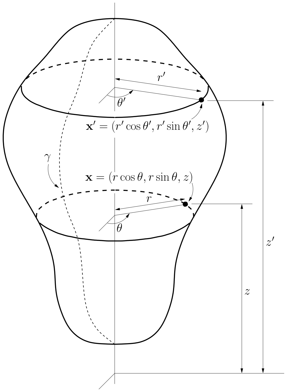
Figure 1. The axisymmetric domain $\Gamma$ generated by the curve $\gamma$.

1.6. Outline

Section 2 provides details on the conversion of a BIE on a rotationally symmetric surface to a sequence of BIEs on a generating curve. Section 3 describes a high order methods for discretizing a BIE on a curve. Section 4 summarizes the algorithm and estimates its computational costs. Section 5 describes how to rapidly evaluate the kernels associated with the Laplace equation, and then Section 6 deals with the Helmholtz case. Section 7 describes other applications of the kernel evaluation techniques. Section 8 illustrates the performance of the proposed method via numerical experiments.

2. Fourier Representation of BIE

Consider the BIE (1) under the assumptions on rotational symmetry stated in Section 1.1 (i.e. $\Gamma$ is a rotationally symmetric surface generated by a curve $\gamma$ and that $k$ is a rotationally symmetric kernel). Cylindrical coordinates $(r,z,\theta)$ are introduced as specified in (3). We write $\Gamma=\gamma\times\mathbb{T}$ where $\mathbb{T}$ is the one-dimensional torus, usually parameterized by $\theta\in(-\pi,\,\pi]$.

2.1. Separation of Variables

We define for $n\in\mathbb{Z}$ the functions $f_{n}$, $\sigma_{n}$, and $k_{n}$ via

(6) $$f_{n}(r,z) =\int_{\mathbb{T}}\frac{e^{-in\theta}}{\sqrt{2\pi}}\,f(\theta,r,z)\,d\theta,$$

(7) $$\sigma_{n}(r,z) =\int_{\mathbb{T}}\frac{e^{-in\theta}}{\sqrt{2\pi}}\,\sigma(\theta,r,z)\,d\theta,$$

(8) $$k_{n}(r,z,r^{\prime},z^{\prime}) =\int_{\mathbb{T}}\frac{e^{-in\theta}}{\sqrt{2\pi}}\,k(\theta,r,z,r^{\prime},z^{\prime})\,d\theta.$$

Formulas (6), (7), and (8) define $f_{n}$, $\sigma_{n}$, and $k_{n}$ as the coefficients in the Fourier series of the functions $f$, $\sigma$, and $k$ about the azimuthal variable,

(9) $$f(\boldsymbol{x}) =\sum_{n\in\mathbb{Z}}\frac{e^{in\theta}}{\sqrt{2\pi}}\,f_{n}(r,z),$$

(10) $$\sigma(\boldsymbol{x}) =\sum_{n\in\mathbb{Z}}\frac{e^{in\theta}}{\sqrt{2\pi}}\,\sigma_{n}(r,z),$$

(11) $$k(\boldsymbol{x},\boldsymbol{x}^{\prime})=k(\theta-\theta^{\prime},r,z,r^{\prime},z^{\prime}) =\sum_{n\in\mathbb{Z}}\frac{e^{in(\theta-\theta^{\prime})}}{\sqrt{2\pi}}\,k_{n}(r,z,r^{\prime},z^{\prime}).$$

To determine the Fourier representation of (1), we multiply the equation by $e^{-in\theta}/\sqrt{2\pi}$ and integrate $\theta$ over $\mathbb{T}$. Equation (1) can then be said to be equivalent to the sequence of equations

(12) $$\sigma_{n}(r,z)+\int_{\gamma\times\mathbb{T}}\left[\int_{\mathbb{T}}\frac{e^{-in\theta}}{\sqrt{2\pi}}\,k(\boldsymbol{x},\boldsymbol{x}^{\prime})\,d\theta\right]\,\sigma(\boldsymbol{x}^{\prime})\,dA(\boldsymbol{x}^{\prime})=f_{n}(r,z),\qquad n\in\mathbb{Z}.$$

Invoking (11), we evaluate the bracketed factor in (12) as

(13) $$\int_{\mathbb{T}}\frac{e^{-in\theta}}{\sqrt{2\pi}}\,k(\boldsymbol{x},\boldsymbol{x}^{\prime})\,d\theta=\int_{\mathbb{T}}\frac{e^{-in\theta}}{\sqrt{2\pi}}\,k(\theta-\theta^{\prime},r,z,r^{\prime},z^{\prime})\,d\theta\\ =e^{-in\theta^{\prime}}\int_{\mathbb{T}}\frac{e^{-in(\theta-\theta^{\prime})}}{\sqrt{2\pi}}\,k(\theta-\theta^{\prime},r,z,r^{\prime},z^{\prime})\,d\theta=e^{-in\theta^{\prime}}\,k_{n}(r,z,r^{\prime},z^{\prime}).$$

Inserting (13) into (12) and executing the integration of $\theta^{\prime}$ over $\mathbb{T}$, we find that (1) is equivalent to the sequence of equations

(14) $$\sigma_{n}(r,z)+\sqrt{2\pi}\int_{\gamma}\,k_{n}(r,z,r^{\prime},z^{\prime})\,\sigma_{n}(r^{\prime},z^{\prime})\,r^{\prime}\,dl(r^{\prime},z^{\prime})=f_{n}(r,z),\hskip 10.00002ptn\in\mathbb{Z}.$$

For future reference, we define for $n\in\mathbb{Z}$ the boundary integral operators $\mathcal{K}_{n}$ via

(15) $$[\mathcal{K}_{n}\,\sigma_{n}](r,z)=\sqrt{2\pi}\int_{\gamma}k_{n}(r,z,r^{\prime},z^{\prime})\,\sigma_{n}(r^{\prime},z^{\prime})\,r^{\prime}\,dl(r^{\prime},z^{\prime}).$$

Then equation (14) can be written

(16) $$\bigl{(}I+\mathcal{K}_{n})\,\sigma_{n}=f_{n},\qquad n\in\mathbb{Z}.$$

When each operator $I+\mathcal{K}_{n}$ is continuously invertible, we write the solution of (1) as

(17) $$\sigma(r,z,\theta)=\sum_{n\in\mathbb{Z}}\frac{e^{in\theta}}{\sqrt{2\pi}}[(I+\mathcal{K}_{n})^{-1}f_{n}](r,z).$$

2.2. Truncation of the Fourier series

When evaluating the solution operator (17) in practice, we will choose a truncation parameter $N$, and evaluate only the lowest $2N+1$ Fourier modes. If $N$ is chosen so that the given function $f$ is well-represented by its lowest $2N+1$ Fourier modes, then in typical environments the solution obtained by truncating the sum (17) will also be accurate. To substantiate this claim, suppose that $\varepsilon$ is a given tolerance, and that $N$ has been chosen so that

(18) $$||f-\sum_{n=-N}^{N}\frac{e^{in\theta}}{\sqrt{2\pi}}f_{n}||\leq\varepsilon,$$

We define an approximate solution via

(19) $$\sigma_{\textrm{approx}}=\sum_{n=-N}^{N}\frac{e^{in\theta}}{\sqrt{2\pi}}(I+\mathcal{K}_{n})^{-1}f_{n}.$$

From Parseval’s identity, we then find that the error in the solution satisfies

$$||\sigma-\sigma_{\textrm{approx}}||^{2}=\sum_{|n|>N}||(I+\mathcal{K}_{n})^{-1}f_{n}||^{2}\leq\sum_{|n|>N}||(I+\mathcal{K}_{n})^{-1}||^{2}\,||f_{n}||^{2}$$

$$\leq\left(\max_{|n|>N}||(I+\mathcal{K}_{n})^{-1}||^{2}\right)\sum_{|n|>N}||f_{n}||^{2}\leq\left(\max_{|n|>N}||(I+\mathcal{K}_{n})^{-1}||^{2}\right)\varepsilon^{2}.$$

It is typically the case that the kernel $k(\boldsymbol{x},\boldsymbol{x}^{\prime})$ has enough smoothness that the Fourier modes $k_{n}(r,z,r^{\prime},z^{\prime})$ decay as $n\rightarrow\infty$. Then $||\mathcal{K}_{n}||\rightarrow 0$ as $n\rightarrow\infty$ and $||(I+\mathcal{K}_{n})^{-1}||\rightarrow 1$. Thus, an accurate approximation of $f$ leads to an approximation in $\sigma$ that is of the same order of accuracy. Figure 4 illustrates how fast this convergence is for Laplace’s equation (note that in the case illustrated, the original equation is $\tfrac{1}{2}\sigma+\mathcal{K}\sigma=f$, and it is shown that $||(\tfrac{1}{2}I+\mathcal{K}_{n})^{-1}||\rightarrow 1/2$).

3. Nyström discretization of BIEs on the generating curve

We discretize the BIEs (5) defined on the generating curve $\gamma$ using a Nyström scheme. In describing the scheme, we keep the formulas uncluttered by discussing a generic integral equation

$$\sigma(\boldsymbol{x})+\int_{\gamma}k(\boldsymbol{x},\boldsymbol{x}^{\prime})\,\sigma(\boldsymbol{x}^{\prime})\,dl(\boldsymbol{x}^{\prime})=f(\boldsymbol{x}),\qquad\boldsymbol{x}\in\gamma,$$

where $\gamma$ is a simple smooth curve in the plane, and $k$ is a weakly singular kernel function.

3.1. Quadrature nodes

Consider a quadrature rule on $\gamma$ with nodes $\{\boldsymbol{x}_{i}\}_{i=1}^{I}\subset\gamma$ and weights $\{w_{i}\}_{i=1}^{I}$. In other words, for a sufficiently smooth function $\varphi$ on $\gamma$,

(20) $$\int_{\gamma}\varphi(\boldsymbol{x})\,dl(\boldsymbol{x})\approx\sum_{i=1}^{I}\varphi(\boldsymbol{x}_{i})\,w_{i}.$$

For the experiments in this paper, we use a composite Gaussian rule with $10$ points per panel. Such a rule admits for local refinement, and can easily be modified to accommodate contours with corners that are only piece-wise smooth.

3.2. A simplistic Nyström scheme

The Nyström discretization of (20) corresponding to a quadrature with nodes $\{\boldsymbol{x}_{i}\}_{i=1}^{I}$ takes the form

(21) $$\sigma_{i}+\sum_{j=1}^{I}a_{i,j}\,\sigma_{j}=f(\boldsymbol{x}_{i}),\qquad i=1,\,2,\,3,\,\dots,\,I,$$

where $\{a_{i,j}\}_{i,j=1}^{I}$ are coefficients such that

(22) $$\int_{\gamma}k(\boldsymbol{x}_{i},\boldsymbol{x}^{\prime})\,\sigma(\boldsymbol{x}^{\prime})\,dl(\boldsymbol{x}^{\prime})\approx\sum_{j=1}^{I}a_{i,j}\,\sigma(\boldsymbol{x}_{j}),\qquad i=1,\,2,\,3,\,\dots,\,I.$$

The solution of (21) is a vector $\boldsymbol{\sigma}=[\sigma_{i}]_{i=1}^{I}$ such that each $\sigma_{i}$ is an approximation to $\sigma(\boldsymbol{x}_{i})$.

A simplistic way to construct coefficients $a_{i,j}$ so that (22) holds is to simply apply the rule (20) to each function $\boldsymbol{x}^{\prime}\mapsto k(\boldsymbol{x}_{i},\boldsymbol{x}^{\prime})\,\sigma(\boldsymbol{x}^{\prime})$ whence

(23) $$a_{i,j}=k(\boldsymbol{x}_{i},\boldsymbol{x}_{j})\,w_{j}.$$

This generally results in low accuracy since the kernel $k(\boldsymbol{x},\boldsymbol{x}^{\prime})$ has a singularity at the diagonal. However, the formula (23) has the great advantage that constructing each $a_{i,j}$ costs no more than a kernel evaluation; we seek to preserve this property for as many elements as possible.

3.3. High-order accurate Nyström discretization

It is possible to construct a high-order discretization that preserves the simple formula (23) for the vast majority of coefficients $a_{i,j}$ [13]. The only coefficients that need to be modified are those for which the target point $\boldsymbol{x}_{i}$ is near the panel $\tau$ holding $\boldsymbol{x}_{j}$. In this case, $a_{i,j}$ is conceptually constructed as follows: First map the pointwise values $\{\sigma_{j}\}_{\boldsymbol{x}_{j}\in\tau}$ to their unique polynomial interpolant on $\tau$, then integrate this polynomial against the singular (or sharply peaked) functions $\boldsymbol{x}^{\prime}\mapsto k(\boldsymbol{x}_{i},\boldsymbol{x}^{\prime})$ using the quadratures of [15] Operationally, the end result is that $a_{i,j}$ is given by

(24) $$a_{i,j}=\left\{\begin{array}[]{ll}\sum_{p=1}^{m}k(\boldsymbol{x}_{i},\boldsymbol{y}_{i,j,p})\,v_{i,j,p}&\mbox{if }\boldsymbol{x}_{i}\mbox{ and }\boldsymbol{x}_{j}\mbox{ are near},\\ k(\boldsymbol{x}_{i},\boldsymbol{x}_{j})\,w_{j}&\mbox{if }\boldsymbol{x}_{i}\mbox{ and }\boldsymbol{x}_{j}\mbox{ are not near}.\end{array}\right.$$

In (24), $m$ is a small integer (roughly equal to the order of the Gaussian quadrature), the numbers $v_{i,j,p}$ are coefficients that depend on $\gamma$ but not on $k$, and $\boldsymbol{y}_{i,j,p}$ are points on $\gamma$ located in the same panel as $\boldsymbol{x}_{j}$ (in fact, $\boldsymbol{y}_{i,j,p}=\boldsymbol{y}_{i,j^{\prime},p}$ when $j$ and $j^{\prime}$ belong to the same panel, so the number of kernel evaluations required is less than it seems). For details, see [13].

4. The full algorithm

4.1. Overview

At this point, we have shown how to convert a BIE defined on an axisymmetric surface in $\mathbb{R}^{3}$ to a sequence of equations defined on a curve in $\mathbb{R}^{2}$ (Section 2), and then how to discretize each of these reduced equations (Section 3). Putting the components together, we obtain the following algorithm for solving (1) to within some preset tolerance $\varepsilon$:

1. Given $f$, determine a truncation parameter $N$ such that $||f-\sum_{n=-N}^{N}\frac{e^{in\theta}}{\sqrt{2\pi}}\,f_{n}||\leq\varepsilon$.

2. Fix a quadrature rule for $\gamma$ with nodes $\{(r_{i},z_{i})\}_{i=1}^{I}\subset\gamma$ and form for each Fourier mode $n=-N,\,-N\,+1,\,-N+2,\,\dots,\,N$ the corresponding Nyström discretization as described in Section 3. The number of nodes $I$ must be picked to meet the computational tolerance $\varepsilon$. Denote the resulting coefficient matrices $\{\mathsf{A}^{(n)}\}_{n=-N}^{N}$.

3. Evaluate via the FFT the terms $\{f_{n}(r_{i},z_{i})\}_{n=-N}^{N}$ (as defined by (6)) for $i=1,\,2,\,3,\,\dots,\,I$.

4. Solve the equation $(\mathsf{I}+\mathsf{A}^{(n)})\,\sigma_{n}=f_{n}$ for $n=-N,\,-N+1,\,-N+2,\,\dots,\,N$.

5. Construct $\sigma_{\rm approx}$ using formula (19) evaluated via the FFT.

The construction of the matrices $\mathsf{A}^{(n)}$ in Step ii can be accelerated using the FFT (as described in Section 4.2), but even with such acceleration, it is typically by a wide margin the most expensive part of the algorithm. However, this step needs to be performed only once for any given geometry. The method therefore becomes particularly efficient when (1) needs to be solved for a sequence of right-hand sides. In this case, it may be worth the cost to pre-compute the inverse (or LU-factorization) of each matrix $\mathsf{I}+\mathsf{A}^{(n)}$.

4.2. Cost of computing the coefficient matrices

For each of the $2N+1$ Fourier modes, we need to construct an $I\times I$ matrix $\mathsf{A}^{(n)}$ with entries $a_{i,j}^{(n)}$. These entries are derived from the kernel functions $k_{n}$ defined by (8). Note that whenever $(r,z)\neq(r^{\prime},z^{\prime})$, the function $\theta\mapsto k(\theta,r,z,r^{\prime},z^{\prime})$ is $C^{\infty}$, but that as $(r^{\prime},z^{\prime})\rightarrow(r,z)$ it develops a progressively sharper peak around $\theta=0$.

For two nodes $(r_{i},z_{i})$ and $(r_{j},z_{j})$ that are “not near” (in the sense defined in Section 3.3) the matrix entries are given by the formula

(25) $$a_{i,j}^{(n)}=k_{n}(r_{i},z_{i},r_{j},z_{j})\,w_{j}$$

where $k_{n}$ is given by (8). Using the FFT, all $2N+1$ entries can be evaluated at once in $O(N\log N)$ operations. The FFT implicitly evaluates the integrals (8) via a trapezoidal rule which is highly accurate since the points $(r_{i},z_{i})$ and $(r_{j},z_{j})$ are well-separated on the curve $\gamma$.

For two nodes $(r_{i},z_{i})$ and $(r_{j},z_{j})$ that are not well-separated on $\gamma$, evaluating $a_{i,j}^{(n)}$ is dicier. The first complication is that we must now use the corrected formula, cf. (24),

(26) $$a_{i,j}^{(n)}=\sum_{p=1}^{m}k_{n}(r_{i},z_{i},r_{i,j,p},z_{i,j,p})\,v_{i,j,p}.$$

The second complication is that the FFT acceleration for computing the kernels $\{k_{n}\}_{n=-N}^{N}$ jointly no longer works since the integrand in (8) is too peaked for the simplistic trapezoidal rule implicit in the FFT. Fortunately, it turns out that for the kernels we are most interested in (the single and double layer kernels associated with the Laplace and Helmholtz equations), the sequence $\{k_{n}\}_{n=-N}^{N}$ can be evaluated very efficiently via certain recurrence relations as described in Sections 5 and 6 (for the Laplace and Helmholtz equations, respectively). Happily, the analytic formulas are stable precisely in the region where the FFT becomes inaccurate.

4.3. Computational Costs

The asymptotic cost of the algorithm described in Section 4.1 will be expressed in terms of the number $N$ of Fourier modes required, and the number $I$ of discretization points required along $\gamma$. The total cost can be split into three components:

1. Cost of forming the matrices $\{\mathsf{A}^{(n)}\}_{n=-N}^{N}$: We need to form $2N+1$ matrices, each of size $I\times I$. For $O(I^{2})$ entries in each matrix, the formula (25) applies and using the FFT, all $2N+1$ entries can be computed at once at cost $O(N\log N)$. For $O(I)$ entries close to the diagonal, the formula (26) applies, and all the $2N+1$ entries can be computed at once at cost $O(N)$ using the recursion relations in Sections 5 and 6. The total cost of this step is therefore $O(I^{2}N\log N)$.

2. Cost of transforming functions from physical space to Fourier space and back: The boundary data $f$ must be decomposed into Fourier modes $\{f_{n}\}_{n=-N}^{N}$, and after the linear systems $(\mathsf{I}+\mathsf{A}^{(n)})\sigma_{n}=f_{n}$ have been solved, the Fourier modes $\{\sigma_{n}\}_{n=-N}^{N}$ must be transformed back to physical space. The asymptotic cost is $O(IN\log(N))$.

3. Cost of solving the linear systems $(\mathsf{I}+\mathsf{A}^{(n)})\,\sigma_{n}=f_{n}$: Using a direct solver such as Gaussian elimination, the asymptotic cost is $O(I^{3}N)$.

We make some practical observations:

• The cost of executing FFTs is minimal and is dwarfed by the remaining costs.

• The scheme is highly efficient in situations where the same equation needs to be solved for a sequence of different right hand sides. In this situation, one factors the matrices $\mathsf{I}+\mathsf{A}^{(n)}$ once at cost $O(I^{3}N)$, and then the cost of processing an additional right hand side is only $O(I^{2}N+IN\log N)$ with a very small constant of proportionality.

• To elucidate the computational costs, let us express them in terms of the total number of discretization points $N_{\rm tot}$ under the simplifying assumption that $I\sim N$. Since $N_{\rm tot}=IN$, we find $I\sim N_{\rm tot}^{1/2}$ and $N\sim N_{\rm tot}^{1/2}$. Then:

  Cost of setting up linear systems:	$O(N_{\rm tot}^{3/2}\log N_{\rm tot})$
  Cost of the first solve:	$O(N_{\rm tot}^{2})$
  Cost of subsequent solves:	$O(N_{\rm tot}^{3/2})$

  We observe that even though the asymptotic cost of forming the linear systems is less than the cost of factoring the matrices, the set-up phase tends to dominate unless $N_{\rm tot}$ is large. Moreover, the $O(N_{\rm tot}^{3/2})$ cost of the subsequent solves has a very small constant of proportionality.

• The high order discretization employed achieves high accuracy with a small number of points. In practical terms, this means that despite the $O(N_{\rm tot}^{2})$ scaling, the scheme is very fast even for moderately complicated geometries.

• The system matrices $\mathsf{I}+\mathsf{A}^{(n)}$ often have internal structure that allow them to be inverted using “fast methods” such as, e.g., those in [18]. The cost of inversion and application can in fact be accelerated to near optimal complexity.

5. Accelerations for the Single and Double Layer Kernels Associated with Laplace’s Equation

This section describes an efficient technique based on recursion relations for evaluating the kernel $k_{n}$, cf. (8), when $k$ is either the single or double layer kernel associated with Laplace’s equation.

5.1. The Double Layer Kernels of Laplace’s Equation

Let $D\subset\mathbb{R}^{3}$ be a bounded domain whose boundary is given by a smooth surface $\Gamma$, let $E=\bar{D}^{\rm c}$ denote the domain exterior to $D$, and let $\boldsymbol{n}$ be the outward unit normal to $D$. Consider the interior and exterior Dirichlet problems of potential theory [11],

(27) $$\Delta u=0\hskip 5.0pt\textrm{in}\hskip 5.0ptD,\hskip 10.00002ptu=f\hskip 5.0pt\textrm{on}\hskip 5.0pt\Gamma,\hskip 20.00003pt$$ (interior Dirichlet problem)

(28) $$\Delta u=0\hskip 5.0pt\textrm{in}\hskip 5.0ptE,\hskip 10.00002ptu=f\hskip 5.0pt\textrm{on}\hskip 5.0pt\Gamma.\hskip 20.00003pt$$ (exterior Dirichlet problem)

The solutions to (27) and (28) can be written in the respective forms

(29) $$u(\boldsymbol{x})=\int_{\Gamma}\frac{\boldsymbol{n}(\boldsymbol{x}^{\prime})\cdot(\boldsymbol{x}-\boldsymbol{x}^{\prime})}{4\pi|\boldsymbol{x}-\boldsymbol{x}^{\prime}|^{3}}\sigma(\boldsymbol{x}^{\prime})\,dA(\boldsymbol{x}^{\prime}),\hskip 10.00002pt\boldsymbol{x}\in D,$$

(30) $$u(\boldsymbol{x})=\int_{\Gamma}\left(-\frac{\boldsymbol{n}(\boldsymbol{x}^{\prime})\cdot(\boldsymbol{x}-\boldsymbol{x}^{\prime})}{4\pi|\boldsymbol{x}-\boldsymbol{x}^{\prime}|^{3}}+\frac{1}{4\pi|\boldsymbol{x}-\boldsymbol{x}_{0}|}\right)\sigma(\boldsymbol{x}^{\prime})\,dA(\boldsymbol{x}^{\prime}),\hskip 10.00002pt\boldsymbol{x}\in E,$$

where $\sigma$ is a boundary charge distribution that can be determined using the boundary conditions. The point $\boldsymbol{x}_{0}$ can be placed at any suitable location in $D$. The resulting equations are

(31) $$-\frac{1}{2}\sigma(\boldsymbol{x}) +\int_{\Gamma}\frac{\boldsymbol{n}(\boldsymbol{x}^{\prime})\cdot(\boldsymbol{x}-\boldsymbol{x}^{\prime})}{4\pi|\boldsymbol{x}-\boldsymbol{x}^{\prime}|^{3}}\sigma(\boldsymbol{x}^{\prime})\,dA(\boldsymbol{x}^{\prime})=f(\boldsymbol{x}),$$

(32) $$-\frac{1}{2}\sigma(\boldsymbol{x}) +\int_{\Gamma}\left(-\frac{\boldsymbol{n}(\boldsymbol{x}^{\prime})\cdot(\boldsymbol{x}-\boldsymbol{x}^{\prime})}{4\pi|\boldsymbol{x}-\boldsymbol{x}^{\prime}|^{3}}+\frac{1}{4\pi|\boldsymbol{x}-\boldsymbol{x}_{0}|}\right)\sigma(\boldsymbol{x}^{\prime})\,dA(\boldsymbol{x}^{\prime})=f(\boldsymbol{x}),$$

where $\boldsymbol{x}\in\Gamma$ in (31) and (32).

Remark 1.

There are other integral formulations for the solution to Laplace’s equation. The double layer formulation presented here is a good choice in that it provides an integral operator that leads to well conditioned linear systems. However, the methodology of this chapter is equally applicable to single-layer formulations that lead to first kind Fredholm BIEs.

5.2. Separation of Variables

Using the procedure given in Section 2, if $\Gamma=\gamma\times\mathbb{T}$, then (27) and (28) can be recast as a series of BIEs defined along $\gamma$. We express $\boldsymbol{n}$ in cylindrical coordinates as

$$\boldsymbol{n}(\boldsymbol{x}^{\prime})=(n_{r^{\prime}}\cos\theta^{\prime},n_{r^{\prime}}\sin\theta^{\prime},n_{z^{\prime}}).$$

Further,

$$|\boldsymbol{x}-\boldsymbol{x}^{\prime}|^{2} =(r\cos\theta-r^{\prime}\cos\theta^{\prime})^{2}+(r\sin\theta-r^{\prime}\sin\theta^{\prime})^{2}+(z-z^{\prime})^{2}$$

$$=r^{2}+(r^{\prime})^{2}-2rr^{\prime}(\sin\theta\sin\theta^{\prime}+\cos\theta\cos\theta^{\prime})+(z-z^{\prime})^{2}$$

$$=r^{2}+(r^{\prime})^{2}-2rr^{\prime}\cos(\theta-\theta^{\prime})+(z-z^{\prime})^{2}$$

and

$$\boldsymbol{n}(\boldsymbol{x}^{\prime})\cdot(\boldsymbol{x}-\boldsymbol{x}^{\prime}) =(n_{r^{\prime}}\cos\theta^{\prime},n_{r^{\prime}}\sin\theta^{\prime},n_{z^{\prime}})\cdot(r\cos\theta-r^{\prime}\cos\theta^{\prime},r\sin\theta-r^{\prime}\sin\theta^{\prime},z-z^{\prime})$$

$$=n_{r^{\prime}}r(\sin\theta\sin\theta^{\prime}+\cos\theta\cos\theta^{\prime})-n_{r^{\prime}}r^{\prime}+n_{z^{\prime}}(z-z^{\prime})$$

$$=n_{r^{\prime}}(r\cos(\theta-\theta^{\prime})-r^{\prime})+n_{z^{\prime}}(z-z^{\prime}).$$

Then for a point $\boldsymbol{x}^{\prime}\in\Gamma$, the kernel of the internal Dirichlet problem can be expanded as

$$\frac{\boldsymbol{n}(\boldsymbol{x}^{\prime})\cdot(\boldsymbol{x}-\boldsymbol{x}^{\prime})}{4\pi|\boldsymbol{x}-\boldsymbol{x}^{\prime}|^{3}}=\frac{1}{\sqrt{2\pi}}\sum_{n\in\mathbb{Z}}e^{in(\theta-\theta^{\prime})}d^{(i)}_{n}(r,z,r^{\prime},z^{\prime}),$$

where

$$d^{(i)}_{n}(r,z,r^{\prime},z^{\prime})=\frac{1}{\sqrt{32\pi^{3}}}\int_{\mathbb{T}}e^{-in\theta}\left[\frac{n_{r^{\prime}}(r\cos\theta-r^{\prime})+n_{z^{\prime}}(z-z^{\prime})}{(r^{2}+(r^{\prime})^{2}-2rr^{\prime}\cos\theta+(z-z^{\prime})^{2})^{3/2}}\right]\,d\theta.$$

Similarly, the kernel of the external Dirichlet problem can be written as

$$-\frac{\boldsymbol{n}(\boldsymbol{x}^{\prime})\cdot(\boldsymbol{x}-\boldsymbol{x}^{\prime})}{4\pi|\boldsymbol{x}-\boldsymbol{x}^{\prime}|^{3}}+\frac{1}{4\pi|\boldsymbol{x}-\boldsymbol{x}_{0}|}=\frac{1}{\sqrt{2\pi}}\sum_{n\in\mathbb{Z}}e^{in(\theta-\theta^{\prime})}d^{(e)}_{n}(r,z,r^{\prime},z^{\prime}),$$

with

$$d^{(e)}_{n}(r,z,r^{\prime},z^{\prime})=\frac{1}{\sqrt{32\pi^{3}}} \int_{\mathbb{T}}e^{-in\theta}\biggl{(}-\frac{n_{r^{\prime}}(r\cos\theta-r^{\prime})+n_{z^{\prime}}(z-z^{\prime})}{(r^{2}+(r^{\prime})^{2}-2rr^{\prime}\cos\theta+(z-z^{\prime})^{2})^{3/2}}+$$

$$+\frac{1}{(r^{2}+r_{0}^{2}-2rr_{0}\cos\theta+(z-z_{0})^{2})^{1/2}}\biggr{)}\,d\theta,$$

where $\boldsymbol{x}_{0}$ has been written in cylindrical coordinates as $(r_{0}\cos(\theta_{0}),r_{0}\sin(\theta_{0}),z_{0})$. With the expansions of the kernels available, the procedure described in Section 4 can be used to solve (31) and (32) by solving

(33) $$\sigma_{n}(r,z)+\sqrt{2\pi}\int_{\gamma}d^{(i)}_{n}(r,r^{\prime},z,z^{\prime})\sigma_{n}(r^{\prime},z^{\prime})\,r^{\prime}\,dl(r^{\prime},z^{\prime})=f_{n}(r,z)$$

and

(34) $$\sigma_{n}(r,z)+\sqrt{2\pi}\int_{\gamma}d^{(e)}_{n}(r,r^{\prime},z,z^{\prime})\sigma_{n}(r^{\prime},z^{\prime})\,r^{\prime}\,dl(r^{\prime},z^{\prime})=f_{n}(r,z),$$

respectively for $n=-N,-N+1,\ldots,N$. Note that the kernels $d^{(i)}_{n}$ and $d^{(e)}_{n}$ contain a log-singularity as $(r^{\prime},z^{\prime})\rightarrow(r,z)$.

5.3. Evaluation of Kernels

The values of $d^{(i)}_{n}$ and $d^{(e)}_{n}$ for $n=-N,-N+1,\ldots,N$ need to be computed efficiently and with high accuracy to construct the Nyström discretization of (33) and (34). Note that the integrands of $d^{(i)}_{n}$ and $d^{(e)}_{n}$ are real valued and even functions on the interval $[-\pi,\pi]$. Therefore, $d^{(i)}_{n}$ can be written as

(35) $$d_{n}^{(i)}(r,z,r^{\prime},z^{\prime})=\frac{1}{\sqrt{32\pi^{3}}}\int_{\mathbb{T}}\left[\frac{n_{r^{\prime}}(r\cos t-r^{\prime})+n_{z^{\prime}}(z-z^{\prime})}{(r^{2}+(r^{\prime})^{2}-2rr^{\prime}\cos t+(z-z^{\prime})^{2})^{3/2}}\right]\cos(nt)\,dt.$$

Note that $d^{(e)}_{n}$ can be written in a similar form.

This integrand is oscillatory and increasingly peaked at the origin as $(r^{\prime},z^{\prime})$ approaches $(r,z)$. As long as $r^{\prime}$ and $r$ as well as $z^{\prime}$ and $z$ are well separated, the integrand does not experience peaks near the origin, and as mentioned before, the FFT provides a fast and accurate way for calculating $d^{(i)}_{n}$ and $d^{(e)}_{n}$.

In regimes where the integrand is peaked, the FFT no longer provides a means of evaluating $d^{(i)}_{n}$ and $d^{(e)}_{n}$ with the desired accuracy. One possible solution to this issue is applying adaptive quadrature to fully resolve the peak. However, this must be done for each value of $n$ required and becomes prohibitively expensive if $N$ is large.

Fortunately, an analytical solution to (35) exists. As noted in [8], the single-layer kernel can be expanded with respect to the azimuthal variable as

$$s(\boldsymbol{x},\boldsymbol{x}^{\prime})=\frac{1}{4\pi|\boldsymbol{x}-\boldsymbol{x}^{\prime}|} =\frac{1}{4\pi(r^{2}+(r^{\prime})^{2}-2rr^{\prime}\cos(\theta-\theta^{\prime})+(z-z^{\prime})^{2})^{1/2}}$$

$$=\frac{1}{\sqrt{2\pi}}\sum_{n\in\mathbb{Z}}e^{in(\theta-\theta^{\prime})}s_{n}(r,z,r^{\prime},z^{\prime}),$$

where

$$s_{n}(r,z,r^{\prime},z^{\prime}) =\frac{1}{\sqrt{32\pi^{3}}}\int_{\mathbb{T}}\frac{\cos(nt)}{(r^{2}+(r^{\prime})^{2}-2rr^{\prime}\cos(t)+(z-z^{\prime})^{2})^{1/2}}\,dt$$

$$=\frac{1}{\sqrt{8\pi^{3}rr^{\prime}}}\int_{\mathbb{T}}\frac{\cos(nt)}{\sqrt{8(\chi-\cos(t))}}\,dt$$

$$=\frac{1}{\sqrt{8\pi^{3}rr^{\prime}}}\mathcal{Q}_{n-1/2}(\chi),$$

$\mathcal{Q}_{n-1/2}$ is the half-integer degree Legendre function of the second kind, and

$$\chi=\frac{r^{2}+(r^{\prime})^{2}+(z-z^{\prime})^{2}}{2rr^{\prime}}.$$

To find an analytical form for (35), first note that in cylindrical coordinates the double-layer kernel can be written in terms of the single-layer kernel,

$$\frac{\boldsymbol{n}(\boldsymbol{x}^{\prime})\cdot(\boldsymbol{x}-\boldsymbol{x}^{\prime})}{4\pi|\boldsymbol{x}-\boldsymbol{x}^{\prime}|^{3}}= \frac{n_{r^{\prime}}(r\cos(\theta-\theta^{\prime})-r^{\prime})+n_{z^{\prime}}(z-z^{\prime})}{4\pi(r^{2}+(r^{\prime})^{2}-2rr^{\prime}\cos(\theta-\theta^{\prime})+(z-z^{\prime})^{2})^{3/2}}$$

$$= \frac{1}{4\pi}\biggl{[}n_{r^{\prime}}\frac{\partial}{\partial r^{\prime}}\left(\frac{1}{(r^{2}+(r^{\prime})^{2}-2rr^{\prime}\cos(\theta-\theta^{\prime})+(z-z^{\prime})^{2})^{1/2}}\right)+$$

$$+n_{z^{\prime}}\frac{\partial}{\partial z^{\prime}}\left(\frac{1}{(r^{2}+(r^{\prime})^{2}-2rr^{\prime}\cos(\theta-\theta^{\prime})+(z-z^{\prime})^{2})^{1/2}}\right)\biggr{]}.$$

The coefficients of the Fourier series expansion of the double-layer kernel are then given by $d^{(i)}_{n}$, which can be written using the previous equation as

$$d_{n}^{(i)}(r,z,r^{\prime},z^{\prime})= n_{r^{\prime}}\int_{\mathbb{T}}\frac{\partial}{\partial r^{\prime}}\left(\frac{\cos(nt)}{(32\pi^{3}(r^{2}+(r^{\prime})^{2}-2rr^{\prime}\cos(t)+(z-z^{\prime})^{2}))^{1/2}}\right)\,dt+$$

$$+n_{z^{\prime}}\int_{\mathbb{T}}\frac{\partial}{\partial z^{\prime}}\left(\frac{\cos(nt)}{(32\pi^{3}(r^{2}+(r^{\prime})^{2}-2rr^{\prime}\cos(t)+(z-z^{\prime})^{2}))^{1/2}}\right)\,dt$$

$$= n_{r^{\prime}}\frac{\partial}{\partial r^{\prime}}\left(\frac{1}{\sqrt{8\pi^{3}rr^{\prime}}}\mathcal{Q}_{n-1/2}(\chi)\right)+n_{z^{\prime}}\frac{\partial}{\partial z^{\prime}}\left(\frac{1}{\sqrt{8\pi^{3}rr^{\prime}}}\mathcal{Q}_{n-1/2}(\chi)\right)$$

$$= \frac{1}{\sqrt{8\pi^{3}rr^{\prime}}}\left[n_{r^{\prime}}\left(\frac{\partial\mathcal{Q}_{n-1/2}(\chi)}{\partial\chi}\frac{\partial\chi}{\partial r^{\prime}}-\frac{\mathcal{Q}_{n-1/2}(\chi)}{2r^{\prime}}\right)+n_{z^{\prime}}\frac{\partial\mathcal{Q}_{n-1/2}(\chi)}{\partial\chi}\frac{\partial\chi}{\partial z^{\prime}}\right].$$

To utilize this form of $d^{(i)}_{n}$, set $\mu=\sqrt{\frac{2}{\chi+1}}$ and note that

$$\frac{\partial\chi}{\partial r^{\prime}}=\frac{(r^{\prime})^{2}-r^{2}-(z-z^{\prime})^{2}}{2r(r^{\prime})^{2}},$$

$$\frac{\partial\chi}{\partial z^{\prime}}=\frac{z^{\prime}-z}{rr^{\prime}},$$

$$\mathcal{Q}_{-1/2}(\chi)=\mu K(\mu),$$

$$\mathcal{Q}_{1/2}(\chi)=\chi\mu K(\mu)-\sqrt{2(\chi+1)}E(\mu),$$

$$\mathcal{Q}_{-n-1/2}(\chi)=\mathcal{Q}_{n-1/2}(\chi),$$

$$\mathcal{Q}_{n-1/2}(\chi)=4\frac{n-1}{2n-1}\chi\mathcal{Q}_{n-3/2}(\chi)-\frac{2n-3}{2n-1}\mathcal{Q}_{n-5/2}(\chi),$$

$$\frac{\partial\mathcal{Q}_{n-1/2}(\chi)}{\partial\chi}=\frac{2n-1}{2(\chi^{2}-1)}\left(\chi\mathcal{Q}_{n-1/2}-\mathcal{Q}_{n-3/2}\right),$$

where $K$ and $E$ are the complete elliptic integrals of the first and second kinds, respectively. The first two relations follow immediately from the definition of $\chi$ and the relations for the Legendre functions of the second kind can be found in [1]. With these relations in hand, the calculation of $d^{(i)}_{n}$ for $n=-N,-N+1,\ldots,N$ can be done accurately and efficiently when $r^{\prime}$ and $r$ as well as $z^{\prime}$ and $z$ are in close proximity. The calculation of $d^{(e)}_{n}$ can be done analogously.

Remark 2.

Note that the forward recursion relation for the Legendre functions $\mathcal{Q}_{n-1/2}(\chi)$ is unstable when $\chi>1$. In practice, the instability is mild when $\chi$ is near $1$ and the recursion relation can still be employed to accurately compute values in this regime. Additionally, if stability becomes an issue, Miller’s algorithm [10] can be used to calculate the values of the Legendre functions using the backwards recursion relation, which is stable for $\chi>1$.

6. Fast Kernel Evaluation for the Helmholtz Equation

Section 5 describes how to efficiently evaluate the kernels $k_{n}$ as defined by (8) for kernels associated with Laplace’s equation. This section generalizes these methods to a broad class of kernels that includes the single and double layer kernels associated with the Helmholtz equation.

6.1. Rapid Kernel Calculation via Convolution

Consider a kernel of the form

(36) $$f(\boldsymbol{x},\boldsymbol{x}^{\prime})=s(\boldsymbol{x},\boldsymbol{x}^{\prime})\,g(\boldsymbol{x},\boldsymbol{x}^{\prime}),$$

where

$$s(\boldsymbol{x},\boldsymbol{x}^{\prime})=\frac{1}{4\pi|\boldsymbol{x}-\boldsymbol{x}^{\prime}|}$$

is the single layer kernel of Laplace’s equation and $g(\boldsymbol{x},\boldsymbol{x}^{\prime})$ is a smooth function for all $\boldsymbol{x},\boldsymbol{x}^{\prime}\in\mathbb{R}^{3}$. Common examples of kernels that take this form include the fundamental solution of the Helmholtz equation and screened Coulomb (Yukawa) potentials.

Letting

$$\boldsymbol{x} =(r\,\cos\theta,\,r\,\sin\theta,\,z),$$

$$\boldsymbol{x}^{\prime} =(r^{\prime}\,\cos\theta^{\prime},\,r^{\prime}\,\sin\theta^{\prime},\,z^{\prime}),$$

we are interested in calculating the Fourier expansion of (36) in terms of the azimuthal variable. When $g(\boldsymbol{x},\boldsymbol{x}^{\prime})=1$ (the Laplace kernel), we know how to rapidly compute these Fourier coefficients rapidly and efficiently. However, when $g$ takes a nontrivial form, this is not generally true; there is no known analytical formula for calculating the Fourier coefficients of (36).

We will now describe an efficient technique for calculating the the Fourier coefficients of (36), when the function $g$ is sufficiently smooth. For a fixed value of $(r,z)$ and $(r^{\prime},z^{\prime})$, the functions $s$ and $g$ are periodic in the azimuthal variable over the interval $\mathbb{T}$. Dropping the dependence of $s$ and $g$ on $(r,z)$ and $(r^{\prime},z^{\prime})$ for notational clarity, we define $t=\theta-\theta^{\prime}\in\mathbb{T}$ and the Fourier series expansions of $s$ and $g$ as

(37) $$s(t) =\sum_{n\in\mathbb{Z}}\frac{e^{int}}{\sqrt{2\pi}}\,s_{n},$$

(38) $$g(t) =\sum_{n\in\mathbb{Z}}\frac{e^{int}}{\sqrt{2\pi}}\,g_{n},$$

where

(39) $$s_{n} =\int_{\mathbb{T}}\frac{e^{-int}}{\sqrt{2\pi}}\,s(t)\,dt,$$

(40) $$g_{n} =\int_{\mathbb{T}}\frac{e^{-int}}{\sqrt{2\pi}}\,g(t)\,dt.$$

The values given by (39) can be calculated as described in Section 5, while the values given by (40) can be rapidly and accurately computed using the FFT.

Assuming the Fourier series defined by (37) and (38) are uniformly convergent, we find

$$f_{n}=\frac{1}{\sqrt{2\pi}}\int_{\mathbb{T}}s(t)\,g(t)\,e^{-int}\,dt=\sum_{k\in\mathbb{Z}}s_{k}\,g_{n-k}=[s_{k}*g_{k}](n),$$

where $s_{k}*g_{k}$ is the discrete convolution of the sequences defined by (39) and (40).

In a practical setting, the Fourier series are truncated to finite length. Assuming that we have kept $-N,-N+1,\ldots,N$ terms, directly calculating the convolution would require $O(N^{2})$ operations. Fortunately, this computation can be accelerated to $O(N\log N)$ operations by employing the discrete convolution theorem and the FFT [6].

Letting $\mathcal{D}$ denote the discrete Fourier transform (DFT), the discrete convolution theorem states that the convolution of two periodic sequences $\{a_{n}\}$ and $\{b_{n}\}$ is related by

$$\mathcal{D}\{a_{n}*b_{n}\}_{k}=\alpha A_{k}B_{k},$$

where $\{A_{n}\}=\mathcal{D}\{a_{n}\}$, $\{B_{n}\}=\mathcal{D}\{b_{n}\}$, and $\alpha$ is a known constant depending upon the length of the periodic sequences and the definition of the DFT. Thus, we can rapidly calculate the convolution of two periodic sequences by taking the FFT of each sequence, computing the pointwise product of the result, and then applying the inverse FFT.

Of course, the sequences that we need to convolute are not periodic. Applying the discrete convolution to the sequences defined by (39) and (40) will not be exact, but the error incurred will be small assuming that the Fourier coefficients decay rapidly and that $N$ is large enough. To see this, assume that

$$s(t) =\sum_{n=-N}^{N}\frac{e^{int}}{\sqrt{2\pi}}\,s_{n},$$

$$g(t) =\sum_{n=-N}^{N}\frac{e^{int}}{\sqrt{2\pi}}\,g_{n}.$$

Then the exact Fourier representation of $f$ can be found by taking the product of these two series, which will be of length $4N+1$. As is well known, the coefficients of this product is given by the discrete convolution of the sequences containing the coefficients of the two series, and these sequences must first be padded with $2N$ zeros. Thus, we can effectively calculate the Fourier coefficients of the function given by (36) by calculating $2N+1$ Fourier coefficients of $s$ and $g$, padding these sequences with zeros, calculating the discrete convolution of these sequences, and truncating the resulting sequence. In practice, padding may not even be required if the Fourier coefficients of $s$ and $g$ decay sufficiently fast.

Note that the procedure described in this section is quite general. The azimuthal Fourier coefficients of many kernels that can be represented as the product of a singular function and a smooth function can be found, assuming that there is an accurate technique for determining the coefficients of the singular function.

6.2. Application to the Helmholtz Equation

In this section, we will apply the fast kernel calculation technique described in Section 6.1 to the exterior Dirichlet problem for the Helmholtz equation. Let $D\subset\mathbb{R}^{3}$ be a bounded domain whose boundary is given by a smooth surface $\Gamma$, let $E=\bar{D}^{\rm c}$ denote the domain exterior to $D$, and let $\boldsymbol{n}$ and be the outward unit normal to $D$. The partial differential equation representing this problem is given by

(41) $$\Delta u+k^{2}u=0\hskip 5.0pt\textrm{in}\hskip 5.0ptE,\hskip 10.00002ptu=f\hskip 5.0pt\textrm{on}\hskip 5.0pt\Gamma,$$

where $k>0$ is the wavenumber, and $u$ satisfies the Sommerfeld radiation condition

(42) $$\lim_{r\rightarrow\infty}r\left(\frac{\partial u}{\partial r}-i\,k\,u\right)=0,$$

where $r=|\boldsymbol{x}|$ and the limit holds uniformly in all directions $\boldsymbol{x}/|\boldsymbol{x}|$. Let the single and double layer potentials for the Helmholtz equation be given by

(43) $$\phi(\boldsymbol{x},\boldsymbol{x}^{\prime}) =\frac{e^{ik|\boldsymbol{x}-\boldsymbol{x}^{\prime}|}}{4\pi|\boldsymbol{x}-\boldsymbol{x}^{\prime}|},\hskip 20.00003pt(\textrm{single layer})$$

(44) $$\frac{\partial\phi(\boldsymbol{x},\boldsymbol{x}^{\prime})}{\partial\boldsymbol{n}(\boldsymbol{x}^{\prime})} =\frac{\boldsymbol{n}(\boldsymbol{x}^{\prime})\cdot(\boldsymbol{x}-\boldsymbol{x}^{\prime})}{4\pi|\boldsymbol{x}-\boldsymbol{x}^{\prime}|^{3}}\left[\left(1-ik|\boldsymbol{x}-\boldsymbol{x}^{\prime}|\right)e^{ik|\boldsymbol{x}-\boldsymbol{x}^{\prime}|}\right].\hskip 20.00003pt(\textrm{double layer})$$

The solution to (41) can be written in terms of the double layer potential,

$$u(\boldsymbol{x})=\int_{\Gamma}\frac{\partial\phi(\boldsymbol{x},\boldsymbol{x}^{\prime})}{\partial\boldsymbol{n}(\boldsymbol{x}^{\prime})}\,\sigma(\boldsymbol{x}^{\prime})\,dA(\boldsymbol{x}^{\prime}),\hskip 10.00002pt\boldsymbol{x}\in E,$$

where $\sigma$ is a boundary charge density that can be determined using the boundary conditions. The resulting boundary integral equation is given by

(45) $$\frac{1}{2}\sigma(\boldsymbol{x})+\int_{\Gamma}\frac{\partial\phi(\boldsymbol{x},\boldsymbol{x}^{\prime})}{\partial\boldsymbol{n}(\boldsymbol{x}^{\prime})}\,\sigma(\boldsymbol{x}^{\prime})\,dA(\boldsymbol{x}^{\prime})=f(\boldsymbol{x}).$$

As is well known, (45) is not always uniquely solvable, even though (41) is uniquely solvable for all $k>0$. A common solution to this is to represent the solution to (41) as a combined single and double layer potential,

$$u(\boldsymbol{x})=\int_{\Gamma}\left(\frac{\partial\phi(\boldsymbol{x},\boldsymbol{x}^{\prime})}{\partial\boldsymbol{n}(\boldsymbol{x}^{\prime})}-i\,\nu\,\phi(\boldsymbol{x},\boldsymbol{x}^{\prime})\right)\,\sigma(\boldsymbol{x}^{\prime})\,dA(\boldsymbol{x}^{\prime}),\hskip 10.00002pt\boldsymbol{x}\in E,$$

where $\nu>0$. We have freedom in choosing $\nu$, see, e.g., [7, 16], for some analysis on this choice. The boundary integral equation we need to solve is

(46) $$\frac{1}{2}\sigma(\boldsymbol{x})+\int_{\Gamma}\left(\frac{\partial\phi(\boldsymbol{x},\boldsymbol{x}^{\prime})}{\partial\boldsymbol{n}(\boldsymbol{x}^{\prime})}-i\,\nu\,\phi(\boldsymbol{x},\boldsymbol{x}^{\prime})\right)\,\sigma(\boldsymbol{x}^{\prime})\,dA(\boldsymbol{x}^{\prime})=f(\boldsymbol{x}).$$

7. Fast evaluation of fundamental solutions in cylindrical coordinates

The techniques for kernel evaluations described in Sections 4.2, 5, and 6 are useful not only for solving BIEs, but for solving the Laplace and Helmholtz equations in a variety of contexts where cylindrical coordinates are effective. To illustrate, observe that the free space equation

(47) $$-\Delta u(\boldsymbol{x})-k^{2}\,u(\boldsymbol{x})=f(\boldsymbol{x}),\qquad\boldsymbol{x}\in\mathbb{R}^{3}$$

has the solution

(48) $$u(\boldsymbol{x})=\int_{\mathbb{R}^{3}}\phi^{(k)}(\boldsymbol{x},\boldsymbol{x}^{\prime})\,f(\boldsymbol{x}^{\prime})\,dA(\boldsymbol{x}^{\prime}).\qquad\boldsymbol{x}\in\mathbb{R}^{3},$$

where $\phi^{(k)}$ is the fundamental solution

$$\phi^{(k)}(\boldsymbol{x})=\frac{e^{ik|\boldsymbol{x}|}}{4\pi|\boldsymbol{x}|}.$$

In cylindrical coordinates, we write (48) as

(49) $$u(\boldsymbol{x})=\sum_{n=-\infty}^{\infty}\frac{e^{in\theta}}{\sqrt{2\pi}}\int_{H}\phi_{n}^{(k)}(r,z,r^{\prime},z^{\prime})f_{n}(r^{\prime},z^{\prime})dA(r^{\prime},z^{\prime})$$

where $H=\{(r,z)\in\mathbb{R}^{2}\,\colon\,r\geq 0\}$ is a half-plane, and where $u_{n}$, $f_{n}$, and $\phi_{n}^{(k)}$ are the Fourier coefficients defined by

$$u(\boldsymbol{x})= \sum_{n=-\infty}^{\infty}\frac{e^{in\theta}}{\sqrt{2\pi}}u_{n}(r,z),$$

$$f(\boldsymbol{x})= \sum_{n=-\infty}^{\infty}\frac{e^{in\theta}}{\sqrt{2\pi}}f_{n}(r,z),$$

$$\phi^{(k)}(\boldsymbol{x},\boldsymbol{x}^{\prime}) =\sum_{n=-\infty}^{\infty}\frac{e^{in(\theta-\theta^{\prime})}}{\sqrt{2\pi}}\phi_{n}^{(k)}(r,z,r^{\prime},z^{\prime}).$$

The kernel $\phi_{n}^{(k)}$ in (49) can be evaluated efficiently using the techniques of Sections 4.2, 5 and 6. If $f$ has a rapidly convergent Fourier series, and if “fast” summation (e.g. the Fast Multipole Method) is used to evaluate the integrals in (49), then very efficient solvers result.

More generally, we observe that the equation (47) can be expressed

(50) $$-\frac{\partial^{2}u_{n}}{\partial^{2}r}-\frac{1}{r}\frac{\partial u_{n}}{\partial r}-\frac{\partial^{2}u_{n}}{\partial^{2}z}+\left(\frac{n^{2}}{r^{2}}-k^{2}\right)u_{n}=f_{n},\qquad n\in\mathbb{Z}.$$

and that the function $\phi_{n}^{(k)}$ is the Green’s function of (50).

8. Numerical Results

This section describes several numerical experiments performed to assess the efficiency and accuracy of the numerical scheme outlined in Section 4.1. The geometries investigated are described in Figure 2. The generating curves were parameterized by arc length, and split into $N_{\rm P}$ panels of equal length. A 10-point Gaussian quadrature has been used along each panel, with the modified quadratures of [15] used to handle the integrable singularities in the kernel. The algorithm was implemented in FORTRAN, using BLAS, LAPACK, and the FFT library provided by Intel’s MKL library. All numerical experiments in this section have been carried out on a Macbook Pro with a 2.4 GHz Intel Core 2 Duo and 4GB of RAM.

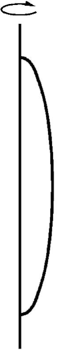
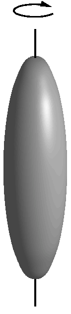
(a)

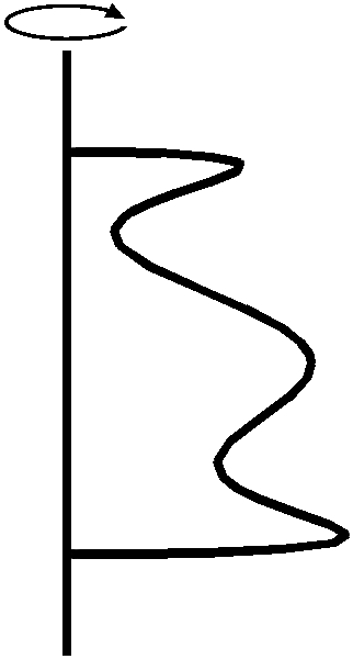
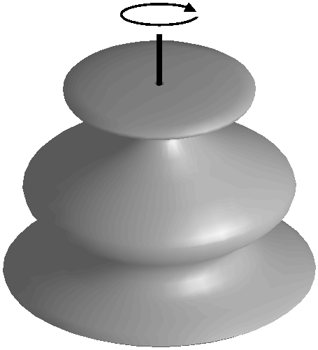
(b)

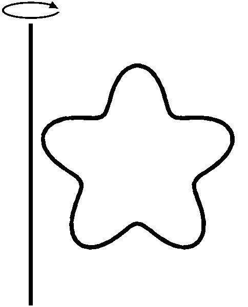
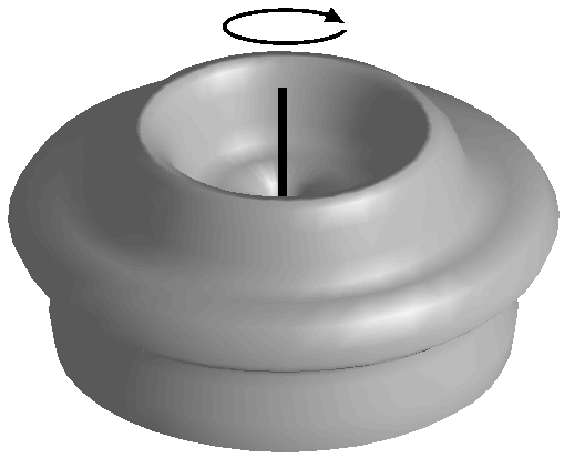
(c)

Figure 2. Domains used in numerical examples. All items are rotated about the vertical axis. (a) An ellipse. (b) A wavy block. (c) A starfish torus.

8.1. Laplace’s equation

We solved Laplace’s equation in the domain interior to the surfaces shown in Figure 2. The solution was represented via the double layer Ansatz (29) leading to the BIE (31). The kernels $d_{n}$ defined via (35) were evaluated using the techniques described in Section 5.3. Tn this case $\mathsf{A}^{(n)}=\mathsf{A}^{(-n)}$, and so we need only to invert $N+1$ matrices. Further, the FFT used here is complex-valued, and a real-valued FFT would yield a significant decrease in computation time.

To investigate the speed of the proposed method, we solved a sequence of problems on the domain in Figure 2(a). The timing results are given in Table 1. The reported results include:

$N_{\rm{P}}$	the number of panels used to discretize the contour (each panel has $I/N_{\rm{P}}$ nodes)
$N$	the Fourier truncation parameter (we keep $2N+1$ modes)
$T_{\textrm{mat}}$	time to construct the linear systems (utilizing the recursion relation)
$T_{\textrm{inv}}$	time to invert the linear systems
$T_{\textrm{fft}}$	time to Fourier transform the right hand side and the solution
$T_{\textrm{apply}}$	time to apply the inverse to the right hand side

The most expensive component of the calculation is the kernel evaluation required to form the coefficient matrices $\mathsf{A}^{(n)}$. Table 2 compares the use of the recursion relation in evaluating the kernel when it is near-singular to using an adaptive Gaussian quadrature. The efficiency of the recursion relation is evident.

Figure 3 plots the time to construct the linear systems as the number of degrees of freedom $N_{\rm tot}=I(2N+1)$ increases, for the case when $I\approx 2N+1$. The estimated asymptotic costs given in this Figure match well with the estimates derived in Section 4.3. It is also clear that as $N_{\rm tot}$ grows, the cost of inversion will eventually dominate. We remark that the asymptotic scaling of this cost can be lowered by using fast techniques for the inversion of boundary integral operators, but that little gain would be achieved for the problem sizes considered here.

We observe that the largest problem reported in Table 1 involves $320\,800$ degrees of freedom. The method requires $1$ minute of pre-computation for this example, and is then capable of computing a solution $u$ from a given data function $f$ in $0.49$ seconds.

$N_{\rm{P}}$	$2N+1$	$T_{\textrm{mat}}$	$T_{\textrm{inv}}$	$T_{\textrm{{fft}}}$	$T_{\textrm{apply}}$
5	25	1.70E-02	1.42E-03	7.81E-05	3.83E-05
10	25	3.64E-02	6.15E-03	1.68E-04	2.66E-04
20	25	9.73E-02	3.52E-02	3.69E-04	2.10E-03
40	25	3.09E-01	2.35E-01	6.69E-04	4.82E-03
80	25	1.20E+00	1.88E+00	1.36E-03	2.85E-02
5	51	2.83E-02	3.02E-03	2.38E-04	1.13E-04
10	51	6.71E-02	1.23E-02	4.48E-04	6.58E-04
20	51	2.02E-01	7.42E-02	9.17E-04	2.63E-03
40	51	7.28E-01	4.94E-01	1.92E-03	1.03E-02
80	51	3.07E+00	3.73E+00	3.59E-03	6.17E-02
5	101	5.08E-02	5.48E-03	7.27E-04	2.38E-04
10	101	1.35E-01	2.27E-02	1.41E-03	1.33E-03
20	101	4.39E-01	1.32E-01	2.73E-03	4.60E-03
40	101	1.98E+00	1.04E+00	6.20E-03	2.14E-02
80	101	7.13E+00	7.04E+00	1.12E-02	1.12E-01
5	201	1.07E-01	1.06E-02	1.80E-03	6.36E-04
10	201	3.33E-01	4.96E-02	3.83E-03	2.79E-03
20	201	1.12E+00	2.73E-01	7.05E-03	9.46E-03
40	201	4.63E+00	1.88E+00	1.46E-02	4.15E-02
80	201	1.71E+01	1.41E+01	2.93E-02	2.15E-01
5	401	1.87E-01	2.15E-02	3.43E-03	1.48E-03
10	401	5.85E-01	9.51E-02	6.59E-03	5.05E-03
20	401	2.15E+00	5.42E-01	1.33E-02	1.91E-02
40	401	8.40E+00	3.71E+00	2.78E-02	7.98E-02
80	401	3.15E+01	2.83E+01	5.56E-02	4.34E-01

Table 1. Timing results in seconds performed for the domain given in Figure 2(a) for the interior Dirichlet problem.

$2N+1$	Composite Quadrature	Recursion Relation
25	1.9	0.017
50	3.1	0.028
100	6.6	0.051
200	18.9	0.107

Table 2. Timing comparison in seconds for constructing the matrices $(\mathsf{I}+\mathsf{A}^{(n)})$ using composite Gaussian quadrature and the recursion relation described in Section 5.3 to evaluate $k_{n}$ for diagonal and near diagonal blocks. The FFT is used to evaluate $k_{n}$ at all other entries. $2N+1$ is the total number of Fourier modes used. 5 panels were used to discretize the boundary.

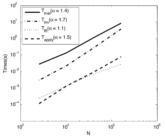
Figure 3. Timings of the algorithm as the number of degrees of freedom $N_{\rm tot}=I(2N+1)$ increases. The timings reported here are for the case $I\approx 2N+1$. The numbers in parentheses provide estimates of the asymptotic complexity, i.e. the best fit to a curve $T=C\,N_{\rm tot}^{\alpha}$.

To test the accuracy of the approach, we have solved a both interior and exterior Dirichlet problems on each of the domains given in Figure 2. Exact solutions were generated by placing a few random point charges outside of the domain where the solution was calculated. The solution was evaluated at points defined on a sphere encompassing (or interior to) the boundary. The errors reported in Tables 3-5 are relative errors measured in the $l^{\infty}$-norm, $||u_{\epsilon}-u||_{\infty}/||u||_{\infty}$, where $u$ is the exact potential and $u_{\epsilon}$ is the potential obtained from the numerical solution.

For all geometries, 10 digits of accuracy has been obtained from a discretization involving a relatively small number of degrees of freedom, due to the rapid convergence of the Gaussian quadrature. This is especially advantageous, as the most expensive component of the algorithm is the construction of the linear systems, the majority of the cost being directly related to the number of panels used. Further, the number of Fourier modes required to obtain 10 digits of accuracy is on the order of 100 modes. Although not investigated here, the discretization technique naturally lends itself to nonuniform refinement in the $rz$-plane, allowing one to resolve features of the generating curve that require finer resolution.

The number of correct digits obtained as the number of panels and number of Fourier modes increases eventually stalls. This is a result of a loss of precision in determining the kernels, as well as cancelation errors incurred when evaluating interactions between nearby points. This is especially prominent with the use of Gaussian quadratures, as points cluster near the ends of the panels. If more digits are required, high precision arithmetic can be employed in the setup phase of the algorithm.

$N_{\rm P}$	$2N+1$
-	25	51	101	201	401
5	3.9506E-04	4.6172E-04	4.6199E-04	4.6203E-04	4.6204E-04
10	1.3140E-05	1.1091E-08	4.8475E-09	4.8480E-09	4.8481E-09
20	1.7232E-05	7.7964E-09	4.7197E-12	4.7232E-12	4.7237E-12
40	2.7527E-05	2.7147E-08	2.8818E-14	5.7173E-14	5.7658E-14
80	2.118E-05	9.4821E-09	2.1529E-13	2.0392E-13	2.0356E-13

Table 3. Error in internal Dirichlet problem solved on domain (a) in Figure 2.

$N_{\rm P}$	$2N+1$
-	25	51	101	201	401
5	8.6992E-04	1.3615E-03	1.3620E-03	1.3621E-03	1.3621E-03
10	2.2610E-04	9.6399E-05	9.6751E-05	9.6751E-05	9.6752E-05
20	2.6291E-04	4.6053E-07	2.4794E-07	2.4794E-07	2.4794E-07
40	3.1714E-04	2.8922E-07	2.2875E-11	2.3601E-11	2.3605E-11
80	3.0404E-04	3.5955E-07	3.3708E-11	3.3138E-11	3.3150E-11

Table 4. Error in external Dirichlet problem solved on domain (b) in Figure 2.

$N_{\rm P}$	$2N+1$
-	25	51	101	201	401
5	4.3633E-04	7.9169E-05	7.8970E-05	7.8970E-05	7.8971E-05
10	3.9007E-04	6.8504E-07	2.0274E-08	2.0272E-08	2.0272E-08
20	3.8803E-04	6.4014E-07	3.2138E-11	3.1624E-11	3.1625E-11
40	3.8456E-04	6.4098E-07	6.5742E-12	3.4529E-12	3.4530E-12
80	3.9828E-04	6.4486E-07	6.8987E-12	3.1914E-12	3.1913E-12

Table 5. Error in external Dirichlet problem solved on domain (c) in Figure 2.

Finally, we investigated the conditioning of the numerical procedure. Figure 4 shows the smallest and largest singular values of the matrices $\{\tfrac{1}{2}\mathsf{I}+\mathsf{A}^{(n)}\}_{n=-200}^{200}$ on the domain shown in Figure 2(a). The convergence of both the smallest and the largest singular values to $1/2$ follow from the convergence $||\mathsf{A}^{(n)}||\rightarrow 0$, cf. Section 2.2. Figure 4 indicates both that all matrices involved are well-conditioned, and that truncation of the Fourier series is generally safe.

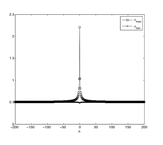
Figure 4. Maximum and minimum singular values for the matrices resulting from an 80 panel discretization of a sphere using 400 Fourier modes, where $n$ is the the matrix associated with the $n^{\textrm{th}}$ Fourier mode.

8.2. Helmholtz Equation

In this section, we repeat many of the experiments reported in Section 8.1, but now for the Helmholtz equation on an exterior domain with the associated “combined field” BIE formulation (46). The algorithm employed to solve the integral equation is the same as described in Section 4, with the caveat that the kernels are calculated using the fast procedure described in Section 6.1.

Table 6 presents timing results, with all variables defined as in Section 8.1.

$N_{\rm{P}}$	$2N+1$	$T_{\textrm{mat}}$	$T_{\textrm{inv}}$	$T_{\textrm{{fft}}}$	$T_{\textrm{apply}}$
5	25	4.51E-02	3.78E-03	2.59E-04	1.77E-04
10	25	1.18E-01	2.03E-02	4.42E-04	8.38E-04
20	25	3.77E-01	1.48E-01	8.47E-04	3.05E-03
40	25	1.27E+00	9.71E-01	1.71E-03	1.19E-02
80	25	5.37E+00	8.20E+00	3.68E-03	8.17E-02
5	51	8.06E-02	6.91E-03	5.09E-04	3.66E-04
10	51	2.25E-01	4.27E-02	1.10E-03	1.00E-03
20	51	7.53E-01	2.85E-01	2.08E-03	6.13E-03
40	51	2.69E+00	1.95E+00	3.83E-03	2.79E-02
80	51	1.01E+01	1.47E+01	7.55E-03	1.40E-01
5	101	1.57E-01	1.36E-02	1.33E-03	8.13E-04
10	101	4.74E-01	8.20E-02	2.55E-03	3.05E-03
20	101	1.58E+00	5.27E-01	5.03E-03	1.17E-02
40	101	5.95E+00	3.81E+00	1.01E-02	5.67E-02
80	101	2.11E+01	2.72E+01	1.90E-02	2.39E-01
5	201	3.02E-01	2.50E-02	2.56E-03	1.64E-03
10	201	9.40E-01	1.56E-01	5.09E-03	5.71E-03
20	201	3.23E+00	1.02E+00	1.01E-02	2.15E-02
40	201	1.19E+01	7.32E+00	2.05E-02	9.94E-02
80	201	4.35E+01	5.38E+01	4.04E-02	4.67E-01
5	401	5.90E-01	5.046E-02	5.66E-03	3.48E-03
10	401	1.86E+00	2.97E-01	1.05E-02	1.06E-02
20	401	6.60E+00	2.04E+00	2.20E-02	4.75E-02
40	401	2.40E+01	1.46E+01	4.42E-02	1.98E-01

Table 6. Timing results in seconds performed for a spherical domain.

The largest problem size considered here has 80 panels and 201 Fourier modes, leading to $160\,800$ unknowns discretizing the surface. Note that this problem size is slightly smaller than the largest considered in Section 8.1, due to memory constraints. This is because the matrices now contain complex entries, and thus use twice the memory compared with the Laplace case. The total running time of the algorithm is 97 seconds for this problem size. If given additional right hand sides, we can solve them in 0.51 seconds. We also remark that the asymptotic scaling of the cost of this algorithm is identical to that of the Laplace case, it simply takes more operations (roughly twice as many) to calculate the kernels and perform the required matrix operations.

We have assessed the accuracy of the algorithm for various domains, discretization parameters, and Fourier modes. The boundary conditions used are determined by placing point charges inside the domains, and we evaluate the solution at random points placed on a sphere that encompasses the boundary. In the combined field BIE (46), we set the parameter $\nu=k$.

$N_{\rm P}$	$2N+1$
-	25	51	101	201	401
5	4.2306E-04	4.0187E-04	4.0185E-04	4.0185E-04	4.0185E-04
10	3.4791E-06	2.3738E-06	2.3759E-06	2.3760E-06	2.376E-06
20	7.8645E-06	4.5707E-09	7.1732E-11	7.1730E-11	7.173E-11
40	1.3908E-05	1.5980E-08	2.9812E-13	3.1500E-13	3.148E-13
80	1.0164E-05	5.4190E-09	4.9276E-13	4.8895E-13	-

Table 7. Relative error in external Helmholtz problem for the domain in Figure 2(a). The domain is 1 wavelength in length (the major axis).

$N_{\rm P}$	$2N+1$
-	25	51	101	201	401
5	2.0516E+00	3.4665E+00	4.1762E+00	4.4320E+00	4.4951E+00
10	2.3847E-01	2.4301E-01	2.4310E-01	2.4312E-01	2.4313E-01
20	1.7792E-02	8.8147E-06	8.8075E-06	8.8081E-06	8.8082E-06
40	1.7054E-02	5.4967E-08	3.7994E-10	3.7999E-10	3.7998E-10
80	1.7302E-02	1.6689E-08	1.8777E-11	1.8782E-11	-

Table 8. Relative error in external Helmholtz problem for the domain in Figure 2(a). The domain is 25 wavelengths in length (the major axis).

First, we consider the ellipsoidal domain given in Figure 2(a). The major axis of this ellipse has a diameter of 2, and its minor axes have a diameter of 1/2. Table 7 lists the accuracy achieved. We achieve 9 digits of accuracy in this problem with 20 panels and 51 Fourier modes. We have not padded the two sequences in the convolution procedure described in Section 6.1, but as more modes are used the tails of the sequence rapidly approach zero, increasing the accuracy of the convolution algorithm utilized to calculate the kernels. Table 8 displays the same data, but with the wavenumber increased so that there are 25 wavelengths along the length of the ellipsoid. We see a minor decrease in accuracy as we would expect, but it only takes 40 panels and 51 Fourier modes to achieve 8 digits of accuracy.

$N_{\rm P}$	$2N+1$
-	25	51	101	201	401
5	2.6874E+00	2.5719E+00	2.5826E+00	2.2374E+00	1.9047E+00
10	1.6351E+00	4.2972E+00	4.6017E+00	1.0380E+00	1.0328E+00
20	4.3666E+00	2.6963E-03	2.6966E-03	2.6967E-03	2.6967E-03
40	4.4498E+00	9.1729E-08	4.1650E-08	4.1661E-08	4.1664E-08
80	4.3692E+00	7.3799E-08	1.4811E-10	1.4812E-10	-

Table 9. Relative error in external Helmholtz problem for the domain in Figure 2(b). The domain is 10 wavelengths in length (the major axis).

$N_{\rm P}$	$2N+1$
-	25	51	101	201	401
5	1.1140E+01	3.2400E+01	3.3885E+01	4.4322E+01	1.6151E+01
10	1.9626E+01	7.7739E+01	6.2931E+01	3.6335E-01	3.6344E-01
20	2.6155E+01	4.9485E+01	2.5796E+01	4.8239E-05	4.8245E-05
40	3.3316E+01	5.0645E+01	2.4330E+01	1.3841E-09	1.3846E-09
80	1.6966E+01	6.0163E+01	2.4354E+01	1.6510E-10	-

Table 10. Relative error in external Helmholtz problem for the domain in Figure 2(c). The domain is 10 wavelengths in length (the major axis).

We now consider the more complex domains given in Figures 2(b) and 2(c). They are a wavy shaped block and a starfish shaped block with the outer diameter of size roughly $1.5$ and $1.0$, respectively. The accuracy for various values of $N_{P}$ and $N$ are given in Table 9 and 10. We achieve 8 digits of accuracy with $40$ panels and $51$ Fourier modes for the wavy block and 9 digits of accuracy with $40$ panels and $201$ Fourier modes for the starfish block.

Acknowledgements: The work reported was supported by NSF grants DMS0748488 and DMS0941476.

References

- [1] M. Abramowitz and I.A. Stegun, Handbook of mathematical functions with formulas, graphs, and mathematical tables, Dover, New York, 1965.
- [2] Bradley K. Alpert, Hybrid gauss-trapezoidal quadrature rules, SIAM J. Sci. Comput. 20 (1999), 1551–1584.
- [3] K. Atkinson, The numerical solution of integral equations of the second kind, Cambridge University Press, Cambridge, 1997.
- [4] A.A. Bakr, The boundary integral equation method in axisymmetric stress analysis problems, Springer-Verlag, Berlin, 1985.
- [5] J. Bremer, A fast direct solver for the integral equations of scattering theory on planar curves with corners, Journal of Computational Physics (2011), no. 0, –.
- [6] B. Briggs and V.E. Henson, The DFT: An owner’s manual for the discrete fourier transform, SIAM, Philadelphia, 1995.
- [7] O.P. Bruno and L.A. Kunyansky, A fast, high-order algorithm for the solution of surface scattering problems: basic implementation, test, and applications, J. Comput. Phys. 169 (2001), 80–110.
- [8] H.S. Cohl and J.E. Tohline, A compact cylindrical green’s function expansion for the solution of potential problems, Astrophys. J. 527 (1999), 86–101.
- [9] J.L. Fleming, A.W. Wood, and W.D. Wood Jr., Locally corrected nyström method for em scattering by bodies of revolution, J. Comput. Phys. 196 (2004), 41–52.
- [10] A. Gil, J. Segura, and N.M. Temme, Numerical methods for special functions, SIAM, Philadelphia, 2007.
- [11] R.B. Guenther and J.W. Lee, Partial differential equations of mathematical physics and integral equations, Dover, New York, 1988.
- [12] A.K. Gupta, The boundary integral equation method for potential problems involving axisymmetric geometry and arbitrary boundary conditions, Master’s thesis, University of Kentucky, 1979.
- [13] S. Hao, P.G. Martinsson, and P. Young, High-order accurate nystrom discretization of integral equations with weakly singular kernels on smooth curves in the plane, 2011, arXiv.org report #1112.6262.
- [14] S. Kapur and V. Rokhlin, High-order corrected trapezoidal quadrature rules for singular functions, SIAM J. Numer. Anal. 34 (1997), 1331–1356.
- [15] P. Kolm and V. Rokhlin, Numerical quadratures for singular and hypersingular integrals, Comput. Math. Appl. 41 (2001), 327–352.
- [16] R. Kress and W.T. Spassov, On the condition of boundary integral operators for the exterior dirichlet problem for the Helmholtz equation, Numer. Math. 42 (1983), 77–95.
- [17] A.H. Kuijpers, G. Verbeek, and J.W. Verheij, An improved acoustic fourier boundary element method formulation using fast fourier transform integration, J. Acoust. Soc. Am. 102 (1997), 1394–1401.
- [18] P.G. Martinsson and V. Rokhlin, A fast direct solver for boundary integral equations in two dimensions, J. Comput. Phys. 205 (2004), 1–23.
- [19] C. Provatidis, A boundary element method for axisymmetric potential problems with non-axisymmetric boundary conditions using fast fourier transform, Engrg. Comput. 15 (1998), 428–449.
- [20] F.J. Rizzo and D.J. Shippy, A boundary integral approach to potential and elasticity problems for axisymmetric bodies with arbitrary boundary conditions, Mech. Res. Commun. 6 (1979), 99–103.
- [21] D.J. Shippy, F.J. Rizzo, and A.K. Gupta, Boundary-integral solution of potential problems involving axisymmetric bodies and nonsymmetric boundary conditions, Developments in Theoretical and Applied Mechanics (J.E. Stoneking, ed.), 1980, pp. 189–206.
- [22] B. Soenarko, A boundary element formuluation for radiation of acoustic waves from axisymmetric bodies with arbitrary boundary conditions, J. Acoust. Soc. Am. 93 (1993), 631–639.
- [23] S.V. Tsinopoulos, J.P. Agnantiaris, and D. Polyzos, An advanced boundary element/fast fourier transform axisymmetric formulation for acoustic radiation and wave scattering problems, J. Acoust. Soc. Am. 105 (1999), 1517–1526.
- [24] W. Wang, N. Atalla, and J. Nicolas, A boundary integral approach for accoustic radiation of axisymmetric bodies with arbitrary boundary conditions valid for all wave numbers, J. Acoust. Soc. Am. 101 (1997), 1468–1478.