Computing Cartograms with Optimal Complexity

Abstract

In a rectilinear dual of a planar graph vertices are represented by simple rectilinear polygons and edges are represented by side-contact between the corresponding polygons. A rectilinear dual is called a cartogram if the area of each region is equal to a pre-specified weight of the corresponding vertex. The complexity of a cartogram is determined by the maximum number of corners (or sides) required for any polygon. In a series of papers the polygonal complexity of such representations for maximal planar graphs has been reduced from the initial 40 to 34, then to 12 and very recently to the currently best known 10. Here we describe a construction with 8-sided polygons, which is optimal in terms of polygonal complexity as 8-sided polygons are sometimes necessary. Specifically, we show how to compute the combinatorial structure and how to refine the representation into an area-universal rectangular layout in linear time. The exact cartogram can be computed from the area-universal rectangular layout with numerical iteration, or can be approximated with a hill-climbing heuristic.

We also describe an alternative construction for Hamiltonian maximal planar graphs, which allows us to directly compute the cartograms in linear time. Moreover, we prove that even for Hamiltonian graphs 8-sided rectilinear polygons are necessary, by constructing a non-trivial lower bound example. The complexity of the cartograms can be reduced to 6 if the Hamiltonian path has the extra property that it is one-legged, as in outer-planar graphs. Thus, we have optimal representations (in terms of both polygonal complexity and running time) for Hamiltonian maximal planar and maximal outer-planar graphs.

1 Introduction

There is a large body of work about representing planar graphs as contact graphs, i.e., graphs whose vertices are represented by geometrical objects with edges corresponding to two objects touching in some specified fashion. Typical classes of objects might be curves, line segments, or polygons. An early result is Koebe’s 1936 theorem [18] that all planar graphs can be represented by touching disks.

In this paper, we consider contact representations of planar graphs, with vertices represented by simple interior-disjoint polygons and adjacencies represented by a non-trivial contact (shared boundary) between the corresponding polygons. We are specifically interested in the rectilinear weighted version where the vertices are represented by simple (axis-aligned) rectilinear polygons. This type of a representation is known as a rectilinear dual of the input planar graph.

In the weighted version, the input is a planar graph $G=(V,E)$ along with a weight function $w:V(G)\rightarrow\mathbb{R}^{+}$ that assigns a weight to each vertex of $G$. A rectilinear dual is called a cartogram if the area of each region is equal to the pre-specified weight of the corresponding vertex. Such representations have practical applications in cartography [24], geography [28] and sociology [15], but also in VLSI Layout and floor-planning [22]. Other applications can be found in visualization of relational data, where using the adjacency of regions to represent edges in a graph can lead to a more compelling visualization than just drawing a line segment between two points [4].

For rectilinear duals (unweighted) and for cartograms (weighted) it is often desirable, for aesthetic, practical and cognitive reasons, to limit the polygonal complexity of the representation, measured by the number of sides (or by the number of corners). Similarly, it is also desirable to minimize the unused area in the representation, also known as holes in floor-planning and VLSI layouts. A given rectilinear dual is area-universal if it can realize a cartogram with any pre-specified set of weights for the vertices of the graph without disturbing the underlying adjacencies and without increasing the polygonal complexity.

With these considerations in mind, we study the problem of constructing area-universal rectilinear duals and show how to compute cartograms with worst-case optimal polygonal complexity and without any holes.

1.1 Related Work

In our paper and in most of the other papers cited here, “planar graph” refers to an inner-triangulated planar graph with a simple outer-face; the former restriction is required if at most three rectilinear polygons are allowed to meet in a point and the latter restriction is customary to achieve that the union of all the polygons in the representation is a rectangle.

Rectilinear duals (unweighted) were first studied in graph theoretic context, and then with renewed interest in the context of VLSI layouts and floor planning. It is known that $8$ sides are sometimes necessary and always sufficient [13, 21, 34].

The case when the rectilinear polygons are restricted to rectangles has been of particular interest and there are several (independent) characterizations of the class of planar graphs that allows such rectangular duals [30, 20, 19]. A historical overview and a summary of the state of the art in the rectangle contact graphs literature can be found in Buchsbaum et al. [4].

In the above results on rectilinear duals and rectangular duals, the areas of the polygons are not considered; that is, these results deal with the unweighted version of the problem. The weighted version dates back to 1934 when Raisz described rectangular cartograms [24]. Algorithms by van Kreveld and Speckmann [31] and Heilmann et al. [14] yield representations with touching rectangles but the adjacencies may be disturbed and there may also be a small distortions of the weights. Recently, Eppstein et al. [11] characterized the class of planar graphs that have area-universal rectangular duals. The construction of the actual cartogram, given the area-universal rectilinear dual and the weight function, can be accomplished using a result by Wimer et al. [33], which in turn requires numerical iteration.

The result of Eppstein et al. above is restricted to planar graphs that have rectangular duals. Going back to the more general rectilinear duals, leads to a series of papers where the main goal has been to reduce the polygonal complexity while respecting all areas and adjacencies. De Berg et al. initially showed that 40 sides suffice [8]. This was later improved to $34$ sides [17]. In a recent paper [3] the polygonal complexity was reduced to 12 sides and even more recently to 10 sides [2].

Side contact representations of planar graphs have also been studied without the restriction to rectilinear polygons. In the unweighted case 6-sided polygons are sometimes necessary and always sufficient [12]. The constructive upper bound relies on convex 6-sided polygons. In the weighted version, where the area of each polygon is prescribed, examples are known for which polygons with 7 sides are necessary [29]. This lower bound is matched by constructive upper bound of 7 sides if holes are allowed [1]. In the same paper it is shown that even allowing arbitrarily high polygonal complexity and holes of arbitrary size, there exist examples with prescribed areas which cannot be represented with convex polygons. If holes are not allowed then the best previously known polygonal complexity is 10, and it is achieved with rectilinear polygons [2].

1.2 Our Results

Recall that the known lower bound on the polygonal complexity even for unweighted rectilinear duals is 8 while the best known upper bound is 10. Here we present the first construction that matches the lower bound. Specifically, our construction produces 8-sided area-universal rectilinear duals in linear time, and is thus optimal in terms of polygonal complexity. The exact cartogram can be computed from the area-universal rectangular layout with numerical iteration, or can be approximated with a hill-climbing heuristic.

For Hamiltonian maximal planar graphs we have an alternative construction which allows us to directly compute cartograms with 8-sided rectilinear polygons in linear time. Moreover, we prove that 8-sided rectilinear polygons are necessary by constructing a non-trivial lower bound example. If the Hamiltonian path has the extra property that it is one-legged, then we can reduce the polygonal complexity and realize cartograms with 6-sided polygons. This can be used to obtain 6-sided cartograms of maximal outer-planar graphs. Thus we have optimal (in terms of both polygonal complexity and running time) representations for Hamiltonian maximal planar and maximal outer-planar graphs.

2 Preliminaries

A planar graph, $G=(V,E)$, is one that has a drawing without crossing in the plane along with an embedding, defined via the cyclic ordering of edges around each vertex. A plane graph is a fixed planar embedding of a planar graph. It splits the plane into connected regions called faces; the unbounded region is the outer-face and all other faces are called interior faces. A planar (plane) graph is maximal if no edge can be added to it without violating planarity. Thus each face of a maximal plane graph is a triangle. A Hamiltonian cycle in a graph $G$ is a simple cycle containing all the vertices of $G$. A graph $G$ is called Hamiltonian if it contains a Hamiltonian cycle.

A set $P$ of closed simple interior-disjoint polygons with an isomorphism $\mathcal{P}:V\rightarrow P$ is a polygonal contact representation of a graph if for any two vertices $u,v\in V$ the boundaries of $\mathcal{P}(u)$ and $\mathcal{P}(v)$ share a non-empty line-segment if and only if $(u,v)$ is an edge. Such a representation is known as a rectilinear dual of the input graph if polygons in $P$ are rectilinear. In the weighted version the input is the graph $G$, along with a weight function $w:V(G)\rightarrow\mathbb{R}^{+}$ that assigns a weight to each vertex of $G$. A rectilinear dual is called a cartogram if the area of each polygon is equal to the pre-specified weight of the corresponding vertex. We define the complexity of a polygon as the number of sides it has. A common objective is to realize a given graph and a set of weights, using polygons with minimal complexity.

2.1 Canonical Orders and Schnyder Realizers

Next we briefly summarize the concepts of a “canonical order” of a planar graph [10] and that of a “Schnyder realizer” [27]. Let $G=(V,E)$ be a maximal plane graph with outer vertices $u$, $v$, $w$ in clockwise order. Then we can compute in linear time [7] a canonical order or shelling order of the vertices $v_{1}=u$, $v_{2}=v$, $v_{3}$, $\ldots$, $v_{n}=w$, which is defined as one that meets the following criteria for every $4\leq i\leq n$.

• The subgraph $G_{i-1}\subseteq G$ induced by $v_{1}$, $v_{2}$, $\ldots$, $v_{i-1}$ is biconnected, and the boundary of its outer face is a cycle $C_{i-1}$ containing the edge $(u,v)$.

• The vertex $v_{i}$ is in the exterior face of $G_{i-1}$, and its neighbors in $G_{i-1}$ form an (at least 2-element) subinterval of the path $C_{i-1}-(u,v)$.

A Schnyder realizer of a maximal plane graph $G$ is a partition of the interior edges of $G$ into three sets $\mathcal{S}_{1}$, $\mathcal{S}_{2}$ and $\mathcal{S}_{3}$ of directed edges such that for each interior vertex $v$, the following conditions hold:

• $v$ has out-degree exactly one in each of $\mathcal{S}_{1}$, $\mathcal{S}_{2}$ and $\mathcal{S}_{3}$,

• the counterclockwise order of the edges incident to $v$ is: entering $\mathcal{S}_{1}$, leaving $\mathcal{S}_{2}$, entering $\mathcal{S}_{3}$, leaving $\mathcal{S}_{1}$, entering $\mathcal{S}_{2}$, leaving $\mathcal{S}_{3}$.

Schnyder proved that any maximal plane graph has a Schnyder realizer and it can be computed in $O(n)$ time [27]. The first condition implies that $\mathcal{S}_{i}$, for $i=1,2,3$ defines a tree rooted at exactly one exterior vertex and containing all the interior vertices such that the edges are directed towards the root. Denote by $\Phi_{k}(v)$ the parent of vertex $v$ in tree $T_{k}$. The following well-known lemma shows a profound connection between canonical orders and Schnyder realizers.

Lemma 2.1

Let $G$ be a maximal plane graph. Then the following hold.

1. A canonical order of the vertices of $G$ defines a Schnyder realizer of $G$, where the outgoing edges of a vertex $v$ are to its first and last predecessor (where “first” is w.r.t. the clockwise order around $v$), and to its highest-numbered successor.

2. A Schnyder realizer with trees $S_{1}$, $S_{2}$, $S_{3}$ defines a canonical order, which is a topological order of the acyclic graph $\mathcal{S}_{1}^{-1}\cup\mathcal{S}_{2}^{-1}\cup\mathcal{S}_{3}$, where $\mathcal{S}_{k}^{-1}$ is the tree $\mathcal{S}_{k}$ with the direction of all its edges reversed.

3 Cartograms with 8-Sided Polygons

In this section we show that 8-sided polygons are always sufficient and sometimes necessary for a cartogram of a maximal planar graph. Our algorithm for constructing 8-sided area-universal rectilinear duals has three main phases. In the first phase we create a contact representation of the graph $G$, where each vertex of $G$ is represented by an upside-down T, i.e., a horizontal segment and a vertical segment. Figures 1(a)-(b) show a maximal planar graph and its contact representation using T’s, where the three ends of each T are marked with arrows. In the second phase we make both the horizontal and vertical segments of each T into thin polygons with $\lambda$ thickness for some $\lambda>0$. We then have a contact representation of $G$ with $T$-shaped polygons as illustrated in Figure 1(c). In the third phase we remove all the unused area in the representation by assigning each (rectangular) hole to one of the polygons adjacent to it, as illustrated in Figure 1(d). We show that the resulting representation is an area-universal rectilinear dual of $G$ with polygonal complexity 8, as illustrated in Figure 1(e).

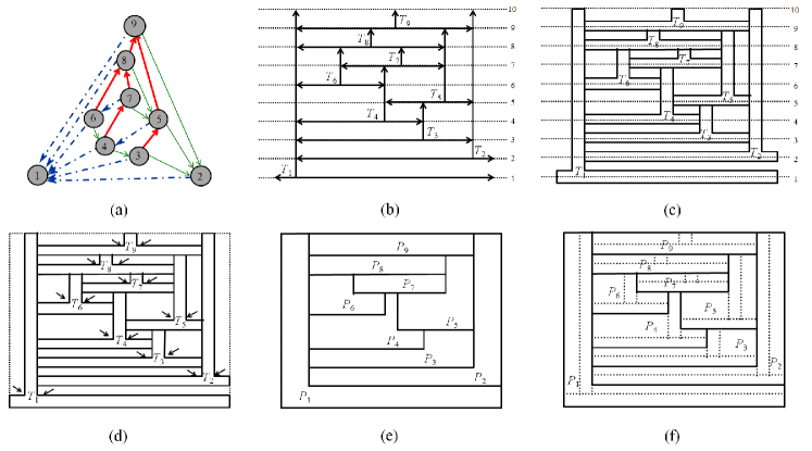
Figure 1: Construction of a rectilinear dual of a maximal planar graph with 8-sided polygons.

3.1 Constructing Contact Representation with T’s

Our contact representation with T’s is similar to the approach described by de Fraysseix et al. [9].

Let $G$ be a planar graph. As mentioned earlier, we may assume that $G$ is internally triangulated and has a simple outer-face. If need be, we can add two vertices (which we later choose as $v_{1}$ and $v_{2}$) and connect them to the outer-face to ensure that the graph is maximal. Now let $v_{1}$, $v_{2}$, $v_{3}$, $\ldots$, $v_{n}$ be a canonical order of the vertices in $G$ with corresponding Schnyder trees $\mathcal{S}_{1}$, $\mathcal{S}_{2}$ and $\mathcal{S}_{3}$ rooted at $v_{1}$, $v_{2}$ and $v_{n}$, Add to $\mathcal{S}_{1}$ the two edges $(v_{2},v_{1})$ and $(v_{n},v_{1})$ oriented towards $v_{1}$ and add to $\mathcal{S}_{2}$ the edge $(v_{n},v_{2})$ oriented towards $v_{2}$. In what follows, we sometimes identify vertex $v_{i}$ with its canonical label $i$.

We assign to vertex $i$ the T-shape $T_{i}$ consisting horizontal and vertical segments $h_{i}$ and $b_{i}$. Begin by placing $T_{1}$ and $T_{2}$ so that $h_{1}$ is placed at $y=1$, $h_{2}$ is placed at $y=2$, the topmost points of both $b_{1}$ and $b_{2}$ have $y$-coordinate $n+1$ and the leftmost point of the $h_{2}$ touches $b_{1}$. Next the algorithm iteratively constructs the contact representation by defining $T_{k}$ so that $h_{k}$ is placed at $y=k$ and the topmost point of $b_{k}$ has $y$-coordinate $\Phi_{3}(k)$ for $3\leq k<n$. After the $k$-th step of the algorithm we have a contact representation of $G_{k}$, and we maintain the invariant that the order of the vertical segments with non-empty parts in the half-plane $y>k$ corresponds to the same circular order of the vertices along $C_{k}-(v_{1},v_{2})$.

Consider inserting $T_{k}$ for $v_{k}$. The neighbors $v_{k_{1}}$, $v_{k_{2}}$, $\ldots$, $v_{k_{d}}$ of $v_{k}$ in $G_{k-1}$ form a subinterval of $C_{k-1}-(v_{1},v_{2})$ and hence the corresponding vertical segments are also in the same order in the half-plane $y>k-1$ of the representation of $G_{k-1}$. Since $v_{k}=\Phi_{3}(v_{k_{i}})$ for $1<i<d$ (Lemma 2.1), the topmost points of the corresponding vertical segments have $y$-coordinate $k$. As $v_{k_{1}}$ and $v_{k_{d}}$ are the parents of $v_{k}$ in $\mathcal{S}_{1}$ and $\mathcal{S}_{2}$, the $x$-coordinates of $b_{k_{1}}$ and $b_{k_{d}}$ define the $x$-coordinates of the two endpoints of $h_{k}$. Let these coordinates be $x_{l}$ and $x_{r}$; then $h_{k}$ is placed between the two points $(x_{l},k)$, $(x_{r},k)$ and $b_{k}$ is placed between the two points $(x_{m},k)$, $(x_{m},\Phi_{3}(k))$ with $x_{l}+1<x_{m}<x_{r}-1$. Finally for $k=n$, we place $T_{n}$ so that $h_{n}$ touches $b_{1}$ to the left and $b_{2}$ to the right and the topmost point of $b_{n}$ has $y$-coordinate $n+1$.

We note here that this representation can be computed in linear time so that all coordinates are integers by pre-computing a topological order $\pi$ of ${\cal S}_{1}^{-1}\cup{\cal S}_{2}$; then $h_{k}$ is the segment $[\pi(\Phi_{1}(k)),\pi(\Phi_{2}(k))]\times k$ and $b_{k}$ is the segment $\pi(k)\times[k,\Phi_{3}(k)]$.

3.2 $\lambda$-Fattening of $T_{i}$’s

Let $\Gamma^{\prime}$ be the contact representation of $G$ using T’s obtained above. In this phase of the algorithm, we “fatten” T’s so that each vertex is represented by a $T$-shaped polygon. We replace each horizontal segment $h_{i}$ by an axis-aligned rectangle $H_{i}$ which has the same width as $h_{i}$, and whose top (bottom) side is $\lambda/2$ above (below) $h_{i}$, for some $0<\lambda$, as illustrated in Figure 2(a). Similarly, we replace each vertical segment $b_{i}$ by an axis-aligned rectangle $B_{i}$ which has the same height as $b_{i}$ and whose left (right) side is $\lambda/2$ to the left (right) of $b_{i}$. We call this process $\lambda$-fattening of $T_{i}$. Note that this process creates intersections of $H_{i}$ with $B_{i}$, $B_{\Phi_{1}(i)}$ and $B_{\Phi_{2}(i)}$ and intersection of $B_{i}$ with $H_{\Phi_{3}(i)}$. We remove these intersections by replacing $H_{i}$ by $H_{i}-B_{\Phi_{1}(i)}-B_{\Phi_{2}(i)}$ and replacing $B_{i}$ by $B_{i}-H_{i}-H_{\Phi_{3}(i)}$. The resulting layout is a contact representation $\Gamma^{\prime\prime}$ of $G$ where each vertex $v_{i}$ of $G$ is represented by the $T$-shaped polygon $H_{i}\cup B_{i}$.

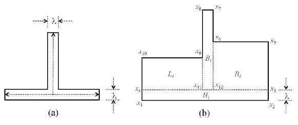
Figure 2: (a) $\lambda$-fattening of $T$, and (b) subdividing a $T$-shaped polygon into four rectangles.

3.3 Removing unused area

In this step, we begin with the $\lambda$-fat $T$-shaped polygonal layout, $\Gamma^{\prime\prime}$, from above and assign each (rectangular) hole to a polygon adjacent to it. We start by placing an axis-aligned rectangle of minimum size that encloses $\Gamma^{\prime\prime}$. This creates five new bounded holes. Note that all the holes in $\Gamma^{\prime\prime}$ are rectangles, and each of them is bounded at the bottom by $H_{i}$ for some vertex $v_{i}$. We assign each hole to this vertex. This assigns at most two holes to each vertex $v_{i}$: one hole $L_{i}$ to the left of $B_{i}$, and one hole $R_{i}$ to the right of $B_{i}$. Now for each vertex $v_{i}$, define $P_{i}=T_{i}\cup L_{i}\cup R_{i}$. It is easy to see that $P_{i}$ is an 8-sided rectilinear polygon since the left side of $L_{i}$ has the same $x$-coordinate as the left side of $H_{i}$ and the right side of $R_{i}$ has the same $x$-coordinate as the right side of $H_{i}$. Thus we have a rectilinear dual, $\Gamma$, of $G$ where each vertex $v_{i}$ is represented by $P_{i}$.

We preferred the above description for the computation of $\Gamma$ since it gives the reader some intuition for the construction. However, we note here that the coordinates of $P_{i}$ could be computed directly, without going through T-shapes and $\lambda$-fattening, using the values $\Phi_{k}(v_{i})$ for $k=1,2,3$ and a topological order $\pi$ of ${\cal S}_{1}^{-1}\cup{\cal S}_{2}$. To this end, we take a topological ordering of the acyclic graph $\mathcal{S}_{1}^{-1}\cup\mathcal{S}_{2}$ and for each vertex $v_{i}\neq v_{n}$, we denote the index of $v_{i}$ in this topological ordering by $\pi(i)$. We can fix the placement of the left and right side of $B_{i}$ at $x$-coordinate $\pi(i)-\lambda/2$ and $\pi(i)+\lambda/2$, respectively. Then for each vertex $v_{i}$, the 8-sided rectilinear polygon $P_{i}$ representing $v_{i}$ is defined as follows.

• The horizontal base segment of $P_{i}$ has $y$-coordinate $i-\lambda/2$ and extends from the left to the right segment (defined below.)

• The horizontal top segment of $P_{i}$ has $y$-coordinate $\Phi_{3}(i)$ (in case of $P_{n}$, the top segment has $y$-coordinate $n+\lambda/2$).

• The vertical left segment of $P_{i}$ has $x$-coordinate $\pi(\Phi_{1}(i))+\lambda/2$ and goes upward from the base segment (in case of $P_{1}$ and $P_{n}$, the left segment has $x$-coordinate $1-\lambda/2$).

• The vertical right segment of $P_{i}$ has $x$-coordinate $\pi(\Phi_{2}(i))-\lambda/2$ and goes upward from the base segment (in case of $P_{2}$ and $P_{n}$, the right segment has $x$-coordinate $n-1+\lambda/2$).

• If $v_{i}$ has no children in $\mathcal{S}_{2}$, then the left segment extends upward until the top segment. Otherwise let $j$ be the vertex in it that comes clockwise after $\Phi_{1}(i)$ in the order of neighbors around $i$. (One can see that $v_{j}$ is the child of $v_{i}$ in $\mathcal{S}_{2}$ with the lowest canonical number.) In this case, the left segment extends upward until $x$-coordinate $j-\lambda/2$, from which point the polygon continues rightward towards the left reflex corner at $\pi(i)-\lambda/2$, and then upward until it meets the top segment.

• If $v_{i}$ has no children in $\mathcal{S}_{1}$, then the right segment extends upward until the top segment. Otherwise let $j$ be the vertex in it that comes counter-clockwise after $\Phi_{2}(i)$ in the order of neighbors around $i$. (One can see that $v_{j}$ is the child of $v_{i}$ in $\mathcal{S}_{1}$ with the lowest canonical number.) In this case, the right segment extends upward until $x$-coordinate $j-\lambda/2$, from which point the polygon continues leftward towards the right reflex corner at $\pi(i)+\lambda/2$, and then upward until it meets the top segment.

Then the union of these $n$ polygons define the rectilinear dual $\Gamma$ of $G$ which is contained inside the rectangle $[1-\lambda/2,n-1+\lambda/2]\times[1-\lambda/2,n+\lambda/2]$. Thus we can compute the representation in linear time, and by scaling the representation by a constat factor, we can make all coordinates to be integers of size $O(n)$.

3.4 Area-Universality

A rectilinear dual $\Gamma$ is area-universal if any assignment of areas to its polygons can be realized by a combinatorially equivalent layout. Eppstein et al. [11] studied this concept for the case when all the polygons are rectangles and the outer-face boundary is also a rectangle (which they call a rectangular layout). They gave a characterization of area-universal rectangular layouts using the concept of “maximal line-segment”. A line-segment of a layout is the union of inner edges of the layout forming a consecutive part of a straight-line. A line-segment that is not contained in any other line-segment is maximal. A maximal line-segment $s$ is called one-sided if it is part of the side of at least one rectangular face, or in other words, if the perpendicular line segments that attach to its interior are all on one side of $s$.

Lemma 3.1

[11] A rectangular layout is area-universal if and only if each maximal segment in the layout is one-sided.

No such characterization is known when some faces are not rectangles. Still we can use the characterization from Lemma 3.1 to show that the rectilinear dual obtained by the algorithm from the previous section is area-universal, with the following Lemma.

Lemma 3.2

Let $\Gamma$ be the rectilinear dual obtained by the above algorithm. Then $\Gamma$ is area-universal.

Proof: To show the area-universality of $\Gamma$, we divide all the polygons in $\Gamma$ into a set of rectangles such that the resulting rectangular layout is area-universal. Specifically, we divide each polygon $P_{i}$ into four rectangles $H_{i}$ $B_{i}$, $L_{i}$ and $R_{i}$ (as defined in the previous subsection) by adding three auxiliary segments: one horizontal and two vertical, as illustrated in Figure 2(b). Any horizontal segment $s$ not on the bounding box belongs to some $H_{i}$ (either top or bottom), and expanding it to its maximum it ends at $B_{\Phi_{1}(v_{i})}$ on the left and $B_{\Phi_{2}(i)}$ on the right. So $s$ is one-sided since it is a side of the rectangle $H_{i}$. Any vertical segment $s$ not on the bounding box belongs to some $B_{i}$ (either left or right), and expanding it to its maximum it ends at $H_{i}$ on the bottom and $H_{\Phi_{3}(i)}$ on the top. So $s$ is one-sided since it is a side of the rectangle $B_{i}$.

Now given any assignment of areas $w:V\rightarrow\mathbb{R}^{+}$ to the vertices $V$ of $G$, we split $w(v_{i})$ arbitrarily into four parts and assign the four values to its four associated rectangles. Since $\Gamma^{*}$ is area-universal, there exists a rectilinear dual of $G$ that is combinatorially equivalent to $\Gamma$ for which these areas are realized. Figure 1(f) illustrates the rectangular layout obtained from the rectilinear dual in Figure 1(e). $\Box$

So for any area-assignment, the rectilinear dual that we found can be turned into a combinatorially equivalent one that respects the area requirements. This proves our main result for maximal planar graphs. Omitting $v_{1}$ and $v_{2}$ from the drawing still results in a cartogram where the union of all polygons is a rectangle, so the result also holds for all planar graphs that are inner triangulated and have a simple outer-face.

Recall that the lower bound on the complexity of polygons in any rectilinear dual (and hence in any cartogram) is 8, as proven by Yeap and Sarrafzadeh [34]. The algorithm described in this section, along with this lower bound leads to our main theorem.

Theorem 3.1

Eight-sided polygons are always sufficient and sometimes necessary for a cartogram of an inner triangulated planar graph with a simple outer-face.

3.5 Feature Size and Supporting Line Set

In addition to optimal polygonal complexity, we point out here that the 8-sided area-universal rectilinear layout constructed with our algorithm maximizes the feature size and reduces the number of supporting lines. Earlier constructions, e.g., [8, 3], often rely on “thin connectors” to maintain adjacencies, whereas our construction does not. Specifically, let $G$ be a maximal planar graph with a prescribed weight function $w:V(G)\rightarrow\mathbb{R}^{+}$. Choose $W$ and $H$ such that $W\times H=A=\sum_{v\in V(G)}w(v)$. We are interested in cartograms within a rectangle of width $W$ and the height $H$. Define $w_{min}=min_{v\in V(G)}w(v)$.

Recall that each vertex $v_{i}$ is represented by the union of at most four rectangles $H_{i}\cup B_{i}\cup R_{i}\cup L_{i}$, with $H_{i}$ and $B_{i}$ non-empty. We can distribute the weight of $v_{i}$ arbitrarily among them. In particular, we can assign zero areas to the rectangles $L_{i}$ and $R_{i}$ and split its weight into two equal parts to $H_{i}$ and $B_{i}$. In this layout each original vertex is represented by rectangles $H_{i}$ and $B_{i}$ whose union is either a rectangle or some fattened $T$ or $L$, and all the necessary contacts remain. Hence we can use this simplified layout to produce the cartogram.

The distribution of the weight of $v_{i}$ in equal parts to $H_{i}$ and $B_{i}$ allows to bound the feature size. The height and width of each rectangle are bounded by $H$ and $W$ respectively. Its weight is at least $w_{min}/2$. Therefore, the height and width of each rectangle is at least $\frac{w_{min}}{2\max\{W,H\}}$. Thus the minimum feature size of the cartogram is at least $\frac{w_{min}}{2\max\{W,H\}}$. This is worst-case optimal, as the polygon with the smallest weight might need to reach from left to right and top to bottom in the representation. We may choose $W=H=\sqrt{A}$. Then the minimum feature size is $\frac{w_{min}}{2\sqrt{A}}$. Furthermore the rectangular layout based on the rectangles $H_{i}$ and $B_{i}$ alone yields a cartogram with at most $2n$ supporting lines, instead of the $3n$ supporting lines in the cartogram based on four rectangles per vertex.

3.6 Computing the Cartogram

The proof of Lemma 3.1 implies an algorithm for computing the final cartogram. Splitting the $T$-shaped polygons into four rectangles and distributing the weights on these rectangles yields an area-universal rectangular dual. This combinatorial structure has to be turned into an actual cartogram, i.e., into a layout respecting the given weights. Wimer et al. [33] gave a formulation of the problem which combines flows and quadratic equations. Eppstein et al. [11] indicated that a solution can be found with a numerical iteration. Alternate methods also exist, based on non-linear programming [26], geometric programming [23], and convex programming [6]. Heuristic hill-climbing schemes converge much quicker and can be used in practice, at the expense of small errors [5, 16, 32].

3.7 Implementation and Experimental Results

We implemented the entire algorithm, along with a force-directed heuristic to compute the final cartogram. We treat each region as a rectilinear “room” containing an amount of “air” equal to the weight assigned to the corresponding vertex. We then simulate the natural phenomenon of air pressure applied to the “walls”, which correspond to the line segment borders in our layout.

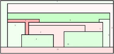
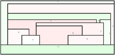
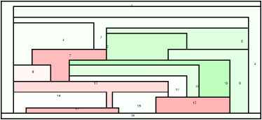
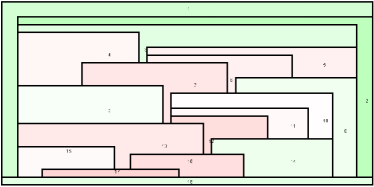
Figure 3: Input-output pairs: weights are assigned at random in the range $[10,100]$, and the cartographic error in the output file is less than 1%. The colors indicate air-pressure: the greener a region is, the more it needs to shrink; the redder a regions is, the more it needs to grow.

For each vertex $v_{i}$ of $G$, the polygon $P_{i}$ contains air with volume $w(v_{i})$. If the area of $P_{i}$ is $A_{i}$, then the pressure applied to each of the walls surrounding $P_{i}$ is given by $\mathcal{P}(v_{i})=\frac{w(v_{i})}{A_{i}}$. In Section 3.4, we saw that the maximal segments of the layout are the two horizontal and the two vertical segment associated with each polygon. For each polygon, the horizontal segment other than the base is entirely inside the polygon, hence it feels no “pressure” on it. For each of the other three segments $s$ for the polygon $P_{i}$, the “inward force” it feels is given by $\mathcal{F}(s)=\sum_{v_{j}\in V(s)}[\mathcal{P}(v_{j})l_{j}]-\mathcal{P}(v_{i})l_{i}$. Here $V(s)$ is the set of vertices other that $v_{i}$ whose corresponding polygon touches the segment $s$ and $l_{i}$ (resp. $l_{j}$) denotes the length of $s$ that is shared with $P_{i}$ (resp. $P_{j}$). At each iteration, we consider the segment that feels the maximum pressure and let it move in the appropriate direction. The convergence of this scheme follows from [16]. Some sample input-output pairs are shown in Fig. 3; more examples and movies showing the gradual transformation can be found at www.cs.arizona.edu/~mjalam/optocart.

We ran a few simple experiments to test the heuristic for time and accuracy. In the first experiment we generated 5 graphs on $n$ vertices with $n$ in the range $[10-50]$ and assigned 5 random weight distributions with weights in the range $[10-100]$. Next we ran the heuristic until the cartographic error dropped below 1% and recorded the average time. All the averages were below 50 milliseconds, which confirms that good solutions can be found very quickly in practice; see Fig 4(a). In the second experiment we fixed the time allowed and tested the quality of the cartograms obtained within the time limit. Specifically, we generated 5 graphs on $n$ vertices with $n$ in the range $[10-50]$ and assigned 5 random weight distributions with weights in the range $[10-100]$. We allowed the program to run for 1 millisecond and recorded the average “cartographic error”. Even with such a small time limit, the average cartographic error was under 2.5%; see Fig. 4(b). Here, the cartographic error for a cartogram of a planar graph $G=(V,E)$ is defined as in [31]: $max_{v\in V}(|A(v)-w(v)|/w(v))$, where $w(v)$ denotes the weight assigned to $v$ and $A(v)$ denotes the area of the polygon representing $v$. All of the experiments were run on an Intel Core i3 machine with a 2.2GHz processor and 4GB RAM.

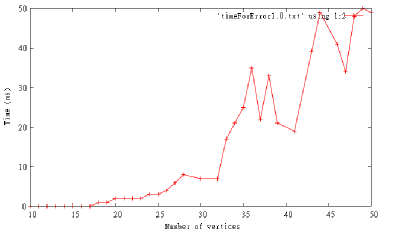
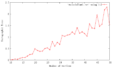
(a)                                                              (b)

Figure 4: Experimental results for graphs with 10-50 vertices. Each sample point corresponds to 25 graphs. (a) Plotting the average time it takes to reach cartographic error of 1%. (b) Plotting the average cartographic error achieved in 1millisecond.

4 Cartograms for Hamiltonian Graphs

In this section we show that 8-sided polygons are always sufficient and sometimes necessary for a cartogram of a Hamiltonian maximal planar graph. We first give a direct linear-time construction with 8-sided regions without relying on numerical iteration or heuristics, as discussed in the previous section. We then prove that this is optimal by showing that 8 sides are necessary, with a non-trivial lower bound example.

4.1 Sufficiency of 8-sided Polygons

Let $v_{1},\dots,v_{n}$ be a Hamiltonian cycle of a maximal planar graph $G$. Consider a plane embedding of $G$ with the edge $(v_{1},v_{n})$ on the triangular outer-face. The Hamiltonian cycle splits the plane graph $G$ into two outer-planar graphs which we call the left graph $G_{l}$ and right graph $G_{r}$. Edges on the Hamiltonian cycle belong to both graphs. The naming is with respect to a planar drawing $\Gamma$ of $G$ in which the vertices $v_{1},\dots,v_{n}$ are placed in increasing order along a vertical line, and the edges are drawn with $y$-monotone curves with leftmost edge $(v_{1},v_{n})$; see Figure 5(a).

Lemma 4.1

Let $G=(V,E)$ be a Hamiltonian maximal planar graph and let $w:V\rightarrow\mathbb{R}^{+}$ be a weight function. Then a cartogram with 8-sided polygons can be computed in linear time.

Proof: Let $v_{1},\ldots,v_{n}$ be a Hamiltonian cycle and $\Gamma$ be the drawing defined above with $(v_{1},v_{n})$ on the outer-face. Suppose $R$ is a rectangle of width $W$ and height $H$ where $W\times H=A=\sum_{v\in V}w(v)$. Each vertex $v_{i}$ will be represented as the union of three rectangles, the left leg, the body $B_{i}$, and right leg of $v_{i}$. We set the width of the legs to $\lambda_{i}=w(v_{i})/(2H+W)$; see Figure 5(b).

Our algorithms places vertices $v_{1},\dots,v_{n}$ in this order, and also reserves vertical strips for legs of all vertices that have earlier neighbors. More precisely, let ${\cal L}_{j}$ be all vertices $v_{k}$ with an edge $(v_{i},v_{k})$ in $G_{l}$ for which $i\leq j<k$. Similarly define ${\cal R}_{j}$ with respect to edges in $G_{r}$. In the drawing $\Gamma$, ${\cal L}_{j}$ are those vertices above $v_{j}$ for which the horizontal ray left from $v_{j}$ crosses an incident edge.

We place vertices $v_{1},\dots,v_{j}$ with the following invariant: The horizontal line through the top of $B_{j}$ intersects, from left to right: (a) a vertical strip of width $\lambda_{k}$ for each $v_{k}\in{\cal L}_{j}$, in descending order, (b) a non-empty part of the top of $B_{j}$, and (c) a vertical strip of width $\lambda_{k}$ for each $v_{k}\in{\cal R}_{j}$, in ascending order.

We start by placing $B_{1}$ as a rectangle that spans the bottom of $R$. At the left and right end of the top of $B_{1}$, we reserve vertical strips of width $\lambda_{k}$ for each vertex in ${\cal L}_{1}$ and ${\cal R}_{1}$, respectively.

To place $B_{i}$, $i>1$, first locate the vertical strips reserved for $v_{i}$ in previous steps (since $v_{i}\in{\cal L}_{i-1}$ and $i\in{\cal R}_{i-1}$, there always are such strips, though they may have started only at the top of $B_{i-1}$). Since vertical strips are in descending/ascending order, the strips for $v_{i}$ are the innermost ones. Let $B_{i}$ be a rectangle just above $B_{i-1}$ connecting these strips. Choose the height of $B_{i}$ so large that it, together with the left and right leg inside the strips, has area $w(v_{i})$; we will discuss soon why this height is positive.

Finally, at the top left of the polygon of $v_{j}$ we reserve a new vertical strip of width $\lambda_{k}$ for each vertex $k$ that is in ${\cal L}_{i}-{\cal L}_{i-1}$. Similarly reserve strips for vertices in ${\cal R}_{i}-{\cal R}_{i-1}$. Using planarity, it is easy to see that vertices in ${\cal L}_{i}-{\cal L}_{i-1}$ must have smaller indices than vertices in ${\cal L}_{i-1}$, and so this can be done such that the order required for the invariant is respected.

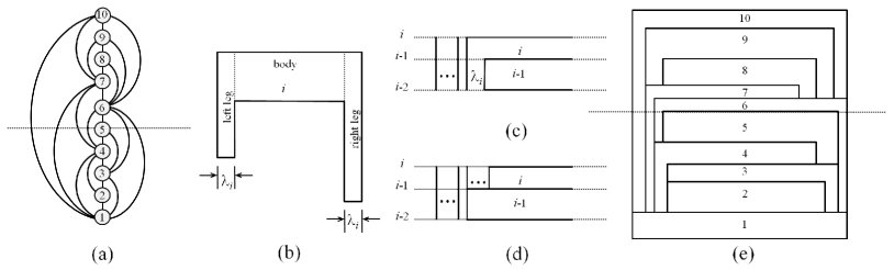
Figure 5: (a) A Hamiltonian maximal planar graph $G$, (b) an 8-sided polygon for vertex $i$, (c)–(d) illustration for the algorithm to construct a cartogram of $G$, (e) a cartogram of $G$ with 8-sided polygons.

Clearly this algorithm takes linear time and constructs 8-gons of the correct area. To see that it creates contacts for all edges, consider an edge $(v_{i},v_{k})$ with $i<k$ in $G_{l}$ (edges in $G_{r}$ are similar.) By definition $k\in{\cal L}_{i}$. If $v_{k}\in{\cal L}_{i}-{\cal L}_{i-1}$, then we reserved a vertical strip for $v_{k}$ when placing $v_{i}$. This vertical strip is used for the left leg of $v_{k}$, which hence touches $v_{i}$. Otherwise ($v_{k}\not\in{\cal L}_{i}-{\cal L}_{i-1}$) we have $v_{k}\in{\cal L}_{i-1}$. At the time that $v_{i-1}$ was placed, there hence existed a vertical strip for $v_{k}$. There also was a vertical strip for $v_{i}\in{\cal L}_{i-1}$. These two strips must be adjacent, because by planarity (and edge $(v_{i},v_{k})$) there can be no vertex $v_{j}$ with $i<j<k$ in ${\cal L}_{i-1}$. So these strips create a contact between the two left legs of $v_{i}$ and $v_{k}$.

We now discuss the choice of $\lambda_{i}=w(v_{i})/(2H+W)$. Each leg of $v_{i}$ has height $\leq H$ and width $\lambda_{i}$, hence area $\leq H\lambda_{i}$. Then the body $B_{i}$ has area $\geq w(v_{i})-2H\lambda_{i}$ and width $\leq W$, hence height $\geq(w(v_{i})-2H\lambda_{i})/W=\lambda_{i}$. It follows that $B_{i}$ has positive height. Also all vertical strips fit: after placing vertex $v_{i}$, we have a strip of width $\lambda_{k}$ for each vertex $v_{k}$ in ${\cal L}_{i}$ and ${\cal R}_{i}$, and these strips use width

$$\sum_{v_{k}\in{\cal L}_{i}}\frac{w(v_{k})}{2H{+}W}+\sum_{v_{k}\in{\cal R}_{i}}\frac{w(v_{k})}{2H{+}W}\leq\frac{2\sum_{v_{k}\in V-\{v_{i}\}}w(v_{k})}{2H{+}W}\leq\frac{2(A-w(v_{i}))}{2H{+}W}\leq\frac{2A}{2H}-\frac{2w(v_{i})}{2H{+}W}=W-2\lambda_{i}.$$

Hence $B_{i}$ has width $\geq 2\lambda_{i}$ and the polygon of $v_{i}$ has minimum feature size $\lambda_{i}$. $\Box$

This algorithm also guarantees a minimum feature size for the cartogram: $\min_{v_{i}\in V}\lambda_{i}=\frac{w_{min}}{2H{+}W}$, where $w_{min}=\min_{v\in V}w(v_{i})$. Choosing $W=\sqrt{2A}$ and $H=\sqrt{A/2}$, yields minimum feature size $\frac{w_{min}}{2\sqrt{2}\sqrt{A}}$.

4.2 Necessity of 8-sided Polygons

While it was known that 8-sided rectilinear polygons are necessary for general planar graphs [25], here we show that 8-sided rectilinear polygons are necessary even for Hamiltonian maximal planar graphs.

Figure 6: (a) A maximal planar Hamiltonian graph with a weight function that requires at least one 8-sided polygon in any cartogram. (b) Illustration for the proof of Lemma 4.2.

Lemma 4.2

Consider the Hamiltonian maximal planar graph $G=(V,E)$ in Figure 6(a). Define $w(j)=w(l)=D$ and $w(v)=\delta$ for $v\in V\setminus\{j,l\}$, where $D\gg\delta$. Then any cartogram of $G$ with weight function $w$ requires at least one 8-sided polygon.

Proof: Assume for a contradiction that $G$ admits a cartogram $\Gamma$ with respect to $w$ such that the polygons $\{P(v)\}$ used in $\Gamma$ have complexity at most 6. Observe that if $\{u,v,x\}$ is some separating triangle in $G$, i.e., three mutually adjacent vertices whose removal disconnect the graph, then the region $R_{uvw}$ used for the inside of the separating triangle contains at least one reflex corner of the polygon $P(u)$, $P(v)$, or $P(x)$. The $5$-vertex set $\{a,c,e,g,i\}$ in $G$ is the union of the five separating triangles $\{a,c,g\}$, $\{a,c,e\}$, $\{c,e,g\}$, $\{a,e,i\}$, and $\{e,g,i\}$ with disjoint interiors. Since all the polygons in $\Gamma$ are either $4$-sided or $6$-sided, the union of the polygons for these five vertices has at most five reflex corners and hence each of the five separating triangles above contains the only reflex corner of the polygon for $a$, $c$, $e$, $g$, or $i$. In particular, the outer boundary of $R_{aei}$ contains exactly one reflex corner from one of $P(a)$, $P(e)$ and $P(i)$, and hence it is a rectangle, say $1234$. By symmetry, we may assume that the reflex corner of $P(i)$ is not used for $R_{aei}$.

The $4$-vertex set $\{a,i,k,m\}$ is the disjoint union of three separating triangles $\{a,k,m\}$, $\{k,i,m\}$, $\{i,a,m\}$ whose interiors are vertices $l,j$ and $n$, respectively. Since the reflex corner of $P(i)$ is not used for $R_{aei}$, it also cannot be used for any of these separating triangles. Hence each of $P(j)$, $P(l)$ and $P(n)$ contains exactly one reflex corner from $P(a)$, $P(k)$ and $P(m)$. In particular, rectangle $1234$ (which is $R_{aei}$) must contain the reflex corner of $P(a)$. We also can conclude that $P(j)$, $P(l)$ and $P(n)$ are all rectangles, since there are no additional reflex corners available to accommodate additional convex corners from $P(j)$, $P(l)$ and $P(n)$.

Assume the naming in Figure 6(b) is such that edge $12$ belongs to $P(i)$, edges $23$ and $34$ belong to $P(a)$ and edge $41$ belongs to $P(e)$. By the adjacencies, $P(k)$ must occupy corners 1 and 4 and $P(n)$ must occupy corner 2, while corner 3 (which is the reflex corner of $P(a)$) could belong to $n$ or $l$.

Now consider the rectangles $P(j)$ and $P(l)$. If $D$ is sufficiently big, then these two rectangles each occupy almost half of rectangle $1234$. Therefore, either their $x$-range or their $y$-range must overlap in their interior. Assume their $y$-range overlaps, the other case is similar. Which polygon should occupy the area that is between $P(j)$ and $P(l)$ horizontally? It cannot be $k$, because $P(k)$ contains corners 1 and 2 and hence would obtain 2 reflex angles from $P(j)$ and $P(l)$. So it must be $P(m)$, since $n$ is not adjacent to $j$ and $l$. But $P(m)$ must also separate $P(n)$ from both $P(j)$ and $P(l)$. Regardless of whether $n$ or $l$ occupies corner 3, this is not possible without two reflex vertices for $m$. Therefore either the areas are not respected or some polygon must have 8 sides. $\Box$

Lemma 4.1 together with Lemma 4.2 yield the following theorem.

Theorem 4.1

Eight-sided polygons are always sufficient and sometimes necessary for a cartogram of a Hamiltonian maximal planar graph.

5 Cartograms with 6-sided Polygons

Here we study cartograms with rectilinear 6-sided polygons. We first note that these are easily constructed for outer-planar graphs. Then we generalize this technique to other maximal planar Hamiltonian graphs.

5.1 Maximal Outer-planar Graphs

Our algorithm from Lemma 4.1 naturally gives drawings of maximal outer-planar graphs that use 6-sided polygons. Another linear-time algorithm for constructing a cartogram of a maximal outer-planar graph with 6-sided rectilinear polygons is also described in [2], however, our construction based on Lemma 4.1 is much simpler. Any maximal outer-planar graph $G$ can be made into a maximal Hamiltonian graph by duplicating $G$ and gluing the copies together at the outer-face such that $G_{l}=G=G_{r}$. (This graph has double edges, but the algorithm in Lemma 4.1 can handle double edges as long as one copy is in the left and one in the right graph.) Create the drawing based on Lemma 4.1 with all vertices having double the weight, and cut it in half with a vertical line. This gives a drawing of $G$ with 6-sided rectilinear polygons as desired.

5.2 One-Legged Hamiltonian Cycles

We now aim to find more maximal Hamiltonian graphs which have cartograms with 6-sided polygons. In a Hamiltonian cycle $v_{1},\ldots,v_{n}$, call vertex $v_{j}$ two-legged if it has a neighbor $v_{i}^{l}$ in $G_{l}$ with $i^{l}<j-1$ and also a neighbor $v_{i}^{r}$ in $G_{r}$ with $i_{r}<j-1$. Call a Hamiltonian cycle one-legged if none of its vertices is two-legged. In the construction from Lemma 4.1, the polygon of $v_{j}$ obtains a reflex vertex on both sides only if it has a neighbor below $v_{j-1}$ on both sides, or in other words, if it is two-legged. Hence we have:

Lemma 5.1

Let $G=(V,E)$ be a maximal planar graph with a one-legged Hamiltonian cycle and let $w:V\rightarrow R^{+}$ be a weight function. Then a cartogram with $6$-sided polygons can be computed in linear time.

It is a natural question to characterize graphs that have such Hamiltonian cycles. Given a Hamiltonian cycle $v_{1},\ldots,v_{n}$ we fix a plane embedding of $G$ with outer triangle $\{v_{1},v_{k},v_{n}\}$. The following lemma gives charecterization of graphs with such hamiltonian cycles.

Lemma 5.2

Let $v_{1},\ldots,v_{n}$ be a Hamiltonian cycle in a maximal plane graph $G$ with $(v_{1},v_{n})$ on the outer triangle. Define $w_{i}:=v_{n-i+1}$. Then the following conditions are equivalent:

1. The Hamiltonian cycle is one-legged.

2. For $i=2,\ldots,n$, edge $(v_{i-1},v_{i})$ is an outer edge of the graph $G_{i}$ induced by by $v_{1},v_{2},\ldots,v_{i}$ (with the induced embedding.)

3. $v_{n-1}$ is an outer vertex and vertex $v_{i}$ has at least two neighbors with a larger index for $i=1,\ldots,n-2$.

4. $w_{1},\ldots,w_{n}$ is a canonical ordering for $G$.

5. $G$ admits a Schnyder realizer $(\mathcal{S}_{1},\mathcal{S}_{2},\mathcal{S}_{3})$ in which $w_{1}$, $w_{2}$ and $w_{n}$ are the roots of $\mathcal{S}_{1}$, $\mathcal{S}_{2}$ and $\mathcal{S}_{3}$, respectively and every inner vertex is a leaf in $\mathcal{S}_{1}$ or $\mathcal{S}_{2}$.

Proof: (a) $\Longleftrightarrow$ (b): For $i=2,\ldots,n$ we argue that (a) vertex $v_{i}$ is not two-legged if and only if (b) holds for $i$. Indeed, $(v_{i-1},v_{i})$ is an inner edge in $G_{i}$ if and only if there are boundary edges $(v_{i},v_{j})$ and $(v_{i},v_{k})$ with $j,k<i-1$ in $G_{l}$ and $G_{r}$, respectively. But then $v_{i}$ is two-legged by definition.

(b) $\Longleftrightarrow$ (c): Since $v_{n}$ is an outer vertex and $G_{n}=G$, (b) holds for $i=n$ if and only if $v_{n-1}$ is an outer vertex. For $i=2,\ldots,n-1$ we argue that (b) holds for $i$ if and only if (c) holds for $i-1$. Let $v_{i}^{l}$, respectively $v_{i}^{r}$, denote the third vertex in the inner facial triangle containing the edge $(v_{i-1},v_{i})$ in $G_{l}$, respectively $G_{r}$. (Both triangles exist, since $(v_{i-1},v_{i})$ is an inner edge in $G$.) Now $(v_{i-1},v_{i})$ is an inner edge in $G_{i}$ if and only if both, $v_{i}^{l}$ and $v_{i}^{r}$, have a smaller index than $v_{i-1}$, which in turn holds if and only if the index of every neighbor of $v_{i-1}$, different from $v_{i}$, is smaller than $i-1$.

(c) $\Longrightarrow$ (d): By (c) $\{w_{1},w_{2},w_{n}\}=\{v_{n},v_{n-1},v_{1}\}$ is the outer triangle of $G$, and moreover, $\tilde{G}_{3}$, which is induced by $v_{n},v_{n-1},v_{n-2}$, is a triangle. Hence the outer boundary of $\tilde{G}_{3}$ is a simple cycle $C_{3}$ containing the edge $(w_{1},w_{2})$. In other words, the first condition of a canonical ordering is met for $i=4$. Assuming (c) and the first condition for $i=4,\ldots,n-1$, we show that the second and first condition holds for $i$ and $i+1$, respectively. In the end, the second condition holds for $i=n$ since $w_{n}$ is an outer vertex.

First note that $w_{i}$ is in the exterior face of $\tilde{G}_{i-1}$ since $w_{n}$ lies in the exterior face and the path $w_{i},\ldots,w_{n}$ is disjoint from vertices in $\tilde{G}_{i-1}$ and the embedding is planar. By (c) $w_{i}$ has at least two neighbors in $\tilde{G}_{i-1}$. If the neighbors would not form a subinterval of the path $C_{i-1}\setminus(w_{1},w_{2})$, there would be a non-triangular inner face in $\tilde{G}_{i}$, which contains a vertex $w_{j}$ with $j>i$ in its interior. But then the path $w_{j},\ldots,w_{n}$, which is disjoint from $\tilde{G}_{i}$, would start and end in an interior and the exterior face of $\tilde{G}_{i}$, respectively. This again contradicts planarity. Thus the second condition of a canonical ordering is satisfied for $i$. Moreover $\tilde{G}_{i}$ is internally triangulated, has a simple outer cycle $C_{i}$ containing the edge $(w_{1},w_{2})$. In other words, the first condition holds for $i+1$.

(d) $\Longrightarrow$ (c): Since $w_{1},\dots,w_{n}$ is a canonical ordering, $(w_{1},w_{2})$ is an outer edge. In particular, $w_{2}=v_{n-1}$ is an outer vertex. Clearly $v_{1}$ has at least two neighbors and every neighbor has a larger index, i.e., (c) holds for $i=1$. Moreover, by the second condition of a canonical ordering every vertex $v_{i}=w_{n-i+1}$, for $i=2,\ldots,n-2$, has at least two neighbors in $\tilde{G}_{n-i}=G\setminus G_{i}$, which is the subgraph induced by $v_{n},\ldots,v_{i+1}$.

(d) $\Longrightarrow$ (e): Consider the Schnyder realizer $(\mathcal{S}_{1},\mathcal{S}_{2},\mathcal{S}_{3})$ of $G$ defined by the canonical order $w_{1},\ldots,w_{n}$ according to Lemma 2.1. For $i=3,\ldots,n-1$ the outer cycle $C_{i}$ of $\tilde{G}_{i}$ consists of the edge $(w_{1},w_{2})$, the $w_{i}w_{1}$-path $P_{1}$ in $\mathcal{S}_{1}$, and the $w_{i}w_{2}$-path $P_{2}$ in $\mathcal{S}_{2}$. Due to the counterclockwise order of edges in a Schnyder realizer, no vertex on $P_{1}$, respectively $P_{2}$, has an incoming inner edge in $\tilde{G}_{i}$ in $\mathcal{S}_{2}$, respectively $\mathcal{S}_{1}$. Thus considering only edges in $\tilde{G}_{i}$ every outer vertex in $\tilde{G}_{i}$, different from $w_{1}$, $w_{2}$, is a leaf in $\mathcal{S}_{1}$ or $\mathcal{S}_{2}$. When in the canonical ordering vertex $w_{i+1}$ is attached to $\tilde{G}_{i}$, some vertices on $C_{i}$ become inner vertices of $\tilde{G}_{i+1}$. Every inner edge in $\tilde{G}_{i+1}$, which was not an edge in $\tilde{G}_{i}$ is in $\mathcal{S}_{3}$. Thus every inner vertex in $\tilde{G}_{i}$ is a leaf in either $\mathcal{S}_{1}$ or $\mathcal{S}_{2}$.

(e) $\Longrightarrow$ (d): Consider a canonical ordering $w_{1},w_{2},\ldots,w_{n}$ of $G$ defined by the Schnyder realizer $(\mathcal{S}_{1},\mathcal{S}_{2},\mathcal{S}_{3})$ according to Lemma 2.1. Then $\{w_{1},w_{2},w_{3}\}$ is a triangle, hence $C_{3}$ consists of the edge $(w_{1},w_{2})$, the $w_{3}w_{1}$-path $P_{1}$ in $\mathcal{S}_{1}$, and the $w_{3}w_{2}$-path $P_{2}$ in $\mathcal{S}_{2}$. For $i=4,\ldots,n$ the vertex $w_{i}$ is attached to $\tilde{G}_{i-1}$. If $w_{i+1}$ would have no edge to $w_{i}$ then the outgoing edge of $w_{i}$ in $\mathcal{S}_{1}$ or $\mathcal{S}_{2}$ is connected an inner vertex in the $w_{i}w_{2}$-path or $w_{i}w_{1}$-path, respectively. But this vertex would then have an incoming edge in both, $\mathcal{S}_{1}$ and $\mathcal{S}_{2}$ – a contradiction. $\Box$

Figure 7 shows an example of a maximal plane graph with a one-legged Hamiltonian cycle, the corresponding canonical ordering, and the Schnyder realizer.

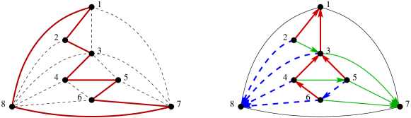
Figure 7: A graph with a one-legged Hamiltonian cycle and the corresponding Schnyder realizer.

Once we have a one-legged Hamiltonian cycle, we can build a 6-sided cartogram via Lemma 5.1 in linear time. Alternately we could obtain from it a Schnyder wood, rooted such that every vertex is a leaf in $\mathcal{S}_{1}$ or $\mathcal{S}_{2}$, and hence obtain a 6-sided cartogram via the algorithm in Section 3. However, we prefer the construction of Lemma 5.1 due to its linear runtime.

We know that not every Hamiltonian maximally planar graph admits a one-legged Hamiltonian cycle; for example, the graph in Figure 6 does not even admit a cartogram with 6-gons. However, we believe that some non-trivial subclasses of Hamiltonian maximally planar graphs are also one-legged Hamiltonian. In particular, we have the following conjecture:

Conjecture 5.1

Every 4-connected maximal planar graph has a one-legged Hamiltonian cycle.

Note that by Lemma 5.2, the conjecture is equivalent to asking whether every 4-connected maximal graph has a Hamiltonian cycle such that taking the vertices in this order gives a canonical ordering. Such a result might be of use for other graph problems as well.

6 Conclusion and Open Problems

We presented a cartogram construction for maximal planar graphs with optimal polygonal complexity. For the precise realization of the actual cartogram this approach requires numerical iteration. Even though the simple heuristic works well in practice, a natural open problem is whether everything can be computed with an entirely combinatorial linear-time approach.

We also presented such an entirely combinatorial linear-time construction for Hamiltonian maximal planar graphs and showed that the resulting 8-sided cartograms are optimal. Finally, we showed that if the graph admits a one-legged Hamiltonian cycle (for example outer-planar graphs), only 6 sides are needed. It remains to identify larger classes of planar graphs which are one-legged Hamiltonian and thus have 6-sided cartograms. We conjecture that 4-connected maximal planar graphs have this property.

All of the constructions in this paper yield area-universal rectilinear duals with optimal polygonal complexity. While Eppstein et al. [11] characterized area-universal rectangular layouts, a similar characterization remains an open problem for general area-universal rectilinear layouts.

For some classes of graphs the unweighted and weighted versions of the problem have the same polygonal complexity, as in the case of general planar graphs where we have shown that the tight bound of 8-sided for weighted graphs matches the tight bound for unweighted graphs. On the other hand, Hamiltonian maximal planar graphs have a tight bound of 6 in the unweighted case, while we have shown that the tight bound is 8 in the weighted case. It would be interesting to study when the weighted version of the problem increases the polygonal complexity.

In a similar vein, rectilinear representations are often desirable for practical and technical reasons (e.g., for VLSI layout or floor-planning). Sometimes, insisting on rectilinear representation increases the underlying polygonal complexity. For example, general (unweighted) planar graphs can be represented by 6-sided polygons (tight bound) while 8 are needed in the rectilinear case. For the weighted version, we also now know that 8 sided are sufficient in the rectilinear case, but can we improve this to 7 sides if we do not insist on rectilinear layouts?

References

- [1] M. J. Alam, T. Biedl, S. Felsner, M. Kaufmann, and S. G. Kobourov. Proportional contact representations of planar graphs. In Graph Drawing (GD 2011), 2011.
- [2] M. J. Alam, T. C. Biedl, S. Felsner, A. Gerasch, M. Kaufmann, and S. G. Kobourov. Linear-time algorithms for hole-free rectilinear proportional contact graph representations. In ISAAC, volume 7074 of LNCS, pages 281–291. Springer, 2011.
- [3] T. Biedl and L. E. Ruiz Velázquez. Orthogonal cartograms with few corners per face. In Data Structures and Algorithms Symposium (WADS’11), volume 6844 of LNCS, pages 98–109. Springer, 2011.
- [4] A. L. Buchsbaum, E. R. Gansner, C. M. Procopiuc, and S. Venkatasubramanian. Rectangular layouts and contact graphs. ACM Transactions on Algorithms, 4(1), 2008.
- [5] I. Cederbaum. Analogy between vlsi floorplanning problems and realisation of a resistive network. IEE Proceedings, Part G, Circuits, Devices and Systems, 139(1):99–103, 1992.
- [6] T. Chen and M. K. H. Fan. On convex formulation of the floorplan area minimization problem. In International Symposium on Physical Design, pages 124–128, 1998.
- [7] M. Chrobak and T. Payne. A linear-time algorithm for drawing planar graphs. Inform. Process. Lett., 54:241–246, 1995.
- [8] M. de Berg, E. Mumford, and B. Speckmann. On rectilinear duals for vertex-weighted plane graphs. Discrete Mathematics, 309(7):1794–1812, 2009.
- [9] H. de Fraysseix, P. O. de Mendez, and P. Rosenstiehl. On triangle contact graphs. Combinatorics, Probability and Computing, 3:233–246, 1994.
- [10] H. de Fraysseix, J. Pach, and R. Pollack. How to draw a planar graph on a grid. Combinatorica, 10(1):41–51, 1990.
- [11] D. Eppstein, E. Mumford, B. Speckmann, and K. Verbeek. Area-universal rectangular layouts. In ACM Symposium on Computational Geometry, pages 267–276. ACM, 2009.
- [12] E. R. Gansner, Y. Hu, M. Kaufmann, and S. G. Kobourov. Optimal polygonal representation of planar graphs. In 9th Latin Am. Symp. on Th. Informatics (LATIN), pages 417–432, 2010.
- [13] X. He. On floor-plan of plane graphs. SIAM Journal of Computing, 28(6):2150–2167, 1999.
- [14] R. Heilmann, D. A. Keim, C. Panse, and M. Sips. Recmap: Rectangular map approximations. In IEEE Symp. on Information Visualization (InfoVis 2004), pages 33–40, 2004.
- [15] D. H. House and C. J. Kocmoud. Continuous cartogram construction. In Proceedings of the conference on Visualization (VIS ’98), pages 197–204, 1998.
- [16] T. Izumi, A. Takahashi, and Y. Kajitani. Air-pressure model and fast algorithms for zero-wasted-area layout of general floorplan. IEICE Transaction on Fundamentals of Electronics, Communications and Computer Sciences, Special Section on Discrete Mathematics and Its Applications, E81–A(5):857–865, 1998.
- [17] A. Kawaguchi and H. Nagamochi. Orthogonal drawings for plane graphs with specified face areas. In 4th Conf. on Theory and Applications of Models of Comp., pages 584–594, 2007.
- [18] P. Koebe. Kontaktprobleme der konformen Abbildung. Berichte über die Verhandlungen der Sächsischen Akademie der Wissenschaften zu Leipzig. Math.-Phys. Klasse, 88:141–164, 1936.
- [19] K. Koźmiński and E. Kinnen. Rectangular duals of planar graphs. Networks, 15:145–157, 1985.
- [20] S. M. Leinwand and Y.-T. Lai. An algorithm for building rectangular floor-plans. In 21st Design Automation Conference, pages 663–664. IEEE Press, 1984.
- [21] C.-C. Liao, H.-I. Lu, and H.-C. Yen. Compact floor-planning via orderly spanning trees. Journal of Algorithms, 48:441–451, 2003.
- [22] J. Michalek, R. Choudhary, and P. Papalambros. Architectural layout design optimization. Engineering Optimization, 34(5):461–484, 2002.
- [23] T.-S. Moh, T.-S. Chang, and S. L. Hakimi. Globally optimal floorplanning for a layout problem. IEEE Transactions on Circuits and Systems I: Fundamental Theory and Applications, 43(9):713–720, 1996.
- [24] E. Raisz. The rectangular statistical cartogram. Geographical Review, 24(3):292–296, 1934.
- [25] I. Rinsma. Nonexistence of a certain rectangular floorplan with specified area and adjacency. Environment and Planning B: Planning and Design, 14:163–166, 1987.
- [26] E. Rosenberg. Optimal module sizing in vlsi floorplanning by nonlinear programming. Methods and Models of Operations Research, 33:131–143, 1989.
- [27] W. Schnyder. Embedding planar graphs on the grid. In ACM-SIAM Symposium on Discrete Algorithms (SODA), pages 138–148, 1990.
- [28] W. Tobler. Thirty five years of computer cartograms. Annals, Assoc. American Geographers, 94:58–73, 2004.
- [29] T. Ueckerdt. Geometric Representations of Graphs with low Polygonal Complexity. PhD thesis, Technische Universität Berlin, 2011.
- [30] P. Ungar. On diagrams representing graphs. J. London Math. Soc., 28:336–342, 1953.
- [31] M. J. van Kreveld and B. Speckmann. On rectangular cartograms. Computational Geometry, 37(3):175–187, 2007.
- [32] K. Wang and W.-K. Chen. Floorplan area optimization using network analogous approach. In IEEE International Symposium on Circuits and Systems, volume 1, pages 167 –170, 1995.
- [33] S. Wimer, I. Koren, and I. Cederbaum. Floorplans, planar graphs, and layouts. IEEE Transactions on Circuits and Systems, 35(3):267 –278, 1988.
- [34] K.-H. Yeap and M. Sarrafzadeh. Floor-planning by graph dualization: 2-concave rectilinear modules. SIAM Journal on Computing, 22:500–526, 1993.