Analysis of wasp-waisted hysteresis loops in magnetic rocks

Abstract

The random-field Ising model of hysteresis is generalized to dilute magnets and solved on a Bethe lattice. Exact expressions for the major and minor hysteresis loops are obtained. In the strongly dilute limit the model provides a simple and useful understanding of the shapes of hysteresis loops in magnetic rock samples.

I Introduction

Hysteresis is a non-equilibrium effect bertotti . If a system is driven by a cyclic force that changes faster than the system can adjust to it, then the response does not move up and down on a single path but rather makes a hysteresis loop. Theoretically the area of the hysteresis loop should vanish as the frequency of the driving field goes to zero but several systems with quenched disorder show large hysteresis even at the slowest driving rate. This behavior arises from the presence of numerous metastable states in the system that are separated from each other by energy barriers much larger than the thermal energy. The metastable states correspond to local minima in the free-energy landscape of the system. The system remains practically trapped in a local minimum and is unable to attain thermal equilibrium over observation times. However, it can be made to jump from one local minimum to another if a sufficiently strong force is applied to it. We focus on magnetic systems. The magnetization induced by a cyclic field traces a hysteresis loop. The loop is essentially a locus of magnetizations of metastable states along the trajectory. Its shape and area are clearly objects of practical interest because these determine the rate of energy dissipation in the system. Somewhat less obvious but equally important is the fact that the hysteresis loop also contains information regarding the distribution of local free-energy minima and the energy barriers between them. Sethna et al introduced the non-equilibrium random-field Ising model of hysteresis that not only reproduces the shapes of hysteresis loops ’pleasantly familiar to the experimentalist’ but also provides an understanding of other aspects associated with it e.g. Barkhausen noise, return point memory, and critical-point phenomena sethna1 ; sethna2 .

Originally the random-field Ising model was introduced to study the effect of quenched positional disorder on the critical behavior of a system in thermal equilibrium  imry-ma . It showed that even an arbitrarily small amount of disorder raises the lower critical dimension of a system. The lower critical dimension is the dimension below which a system can not possess long-range order in a state of thermal equilibrium. Above its lower critical dimension, it may evolve into an ordered state at low temperatures but its approach to thermal equilibrium is not smooth. This is due to the presence of a large number of local minima in the free-energy landscape of disordered systems  young . The local minima are surrounded by high barriers. The barrier heights are random but much higher than the thermal energy of the system. Hence the approach to thermal equilibrium is very slow and sporadic. Indeed the system may not reach equilibrium over practical time scales. This makes the determination of the equilibrium state (the global minimum of free-energy) a difficult task numerically as well as analytically. The dynamics of the approach to thermal equilibrium in the random-field Ising model has been well studied  villain ; dsfisher but the progress has been slow due to the difficulty of the problem.

The difficulty of thermal equilibration is sidelined if the model is used to study hysteresis. Practically speaking, even in the zero frequency limit of the driving field, hysteresis is observed over time periods that are much shorter than the time required for the system to equilibrate. Thus the thermal relaxation process and the global minimum of the free-energy are not of primary importance in this case. In the non-equilibrium random-field Ising model proposed by Sethna et al  sethna1 , the time required by the system to equilibrate is set equal to infinity. Equivalently, the temperature of the system is set equal to zero. The metastable states under the stochastic thermal dynamics thus become stable states under the athermal zero-temperature deterministic dynamics. This does not compromise with the essential physics of the problem. There is an argument based on the renormalization group theory that the phase transition in the equilibrium random-field Ising model is controlled by a stable zero-temperature fixed point dsfisher . Several key features of hysteresis observed in disordered ferromagnets as well other systems whose dynamics is characterized by avalanches are very well reproduced qualitatively and even quantitatively by the zero-temperature non-equilibrium random field Ising model sethna3 . The deterministic dynamics also makes the model amenable to an exact solution in some special cases dhar ; shukla ; shukla2 .

This paper generalizes the non-equilibrium random-field model of hysteresis to dilute magnetic systems. We solve the dilute version of the model exactly on a Bethe lattice and apply the results to explain the shapes of hysteresis loops of magnetic rocks. We choose magnetic rocks for two reasons: (i) these are natural realizations of very dilute magnetic systems, and (ii) have not received the same attention in the physics literature as in geology. It is recognized that rock magnetism arises from a few percent or less of magnetic minerals present in the rocks dunlop1 ; dunlop2 . The commonly occurring magnetic minerals are magnetite ($Fe_{3}O_{4}$), maghemite ($\gamma Fe_{2}O_{3}$), titanomagnetite ($Fe_{2-y}Ti_{y}O_{3}$), pyrrhotite ($Fe_{7}S_{8}$), greigite ($Fe_{3}S_{4}$), hematite ($\alpha Fe_{2}O_{3}$), and goethite ($FeOOH$). The composition note is generally determined by breaking the rock sample. Recently, hysteresis measurements have been employed as a a possible nondestructive alternative. The motivation for this comes from the fact that the hysteresis loop of a rock sample as a whole is generally different from that of its magnetic constituents in their pure form. Pure magnetic minerals are mostly ferromagnetic or ferrimagnetic and therefore their hysteresis loops are similar to those of iron ($Fe$). On the other hand, hysteresis loop of a rock sample as a whole can have unusual shapes including a wasp-waisted shape that is constricted in the middle roberts1 ; roberts2 ; tauxe1 . The wasp-waisted shape is thought to arise from the fact that the grains dispersed in the rock have a distribution of sizes, domain states, and coercive fields roberts1 ; roberts2 ; tauxe1 ; wasilewski ; becker ; pick1 ; pick2 ; bean ; hejda ; bennett ; davies ; tauxe2 ; kletetschka . One would like to determine the distribution of magnetic grains from the hysteresis loop of the rock sample. It is not immediately obvious if this is feasible. A given distribution of grains and a set of interactions between them will produce a unique hysteresis loop. However, the inverse relationship of the hysteresis loop to the contents of the rock is not necessarily unique. This is because the detailed information concerning the grains has to be integrated over in order to obtain the hysteresis loop. Nevertheless there are practical advantages in exploring the extent to which we can deduce the composition of a rock from its hysteresis loop. As a first step towards this goal, one would like to study simple models of hysteresis and explore how their predictions vary with the parameters of the model.

There are a number of models of hysteresis in magnetic rocks in the field of geology. The majority of these use qualitatively similar assumptions and differ from each other only in detail. As an illustration we consider the model studied in reference  tauxe1 . Grains of magnetic minerals of various sizes are assumed to be randomly dispersed in the rock. The grains are frozen in their positions but their magnetization can rotate or flip under a driving field as well as under thermal fluctuations. Interactions between the grains are neglected. This is presumably justified because the grains occupy only a few percent of the total volume of the sample and therefore they may be well separated from each other to interact significantly. The size of a grain determines the quality of its response to the applied field. Small grains (say 30 nm or less) behave like a paramagnet and respond to a cyclic field without hysteresis. Larger grains behave like a ferromagnet and respond to the cyclic field with hysteresis. This is because the size of the grain is related to the size of the energy barriers that stand in the way of smooth rotation or flipping of magnetization within a grain. These barriers are small for small grains and large for large grains. The thermal energy of the system provides the criterion for deciding whether a grain is small or large. If the barriers are small in comparison with the thermal energy, the magnetization is able to rotate freely under thermal fluctuations and is able to attain thermal equilibrium. In this situation the average magnetization is zero in zero applied field. In a non-zero applied field it is given by the Langevin function for a paramagnet. Larger grains are not able to attain thermal equilibrium over time scales of the experiment. Their response to the cyclic field is the non-equilibrium response in the form of a hysteresis loop. A hysteresis loop may be characterized by a number of parameters such as the saturation magnetization, the remanent magnetization, and the coercive field. These parameters are related to the size, shape and material of the grain. Some variants of the model of hysteresis in a rock sample consider directly a distribution of the coercivities of the grains, others a distribution of the sizes that is translated into coercivities through an assumed relationship between the two. The task of the models is to reproduce the experimentally observed shapes of hysteresis loops for a reasonable choice of the parameters of the model. Some models achieve this task by considering grains of different sizes  tauxe1 ; bean , others by strongly contrasting coercivities  wasilewski ; roberts1 . A few models have also included interactions between the grains  bennett ; hejda ; davies . A number of models reproduce major hysteresis loops similar to those observed in the laboratory experiments. Thus the difficulty is not that we do not have a model of rock magnetism but that we have several. The question naturally arises if we can distinguish between these models. Some authors have suggested that the comparison of experimental first-order reversal curves (minor hysteresis loops) with the predictions of different models may serve to distinguish between them bennett .

As stated earlier, we adapt the non-equilibrium random-field model of hysteresis to dilute magnets. It offers a framework for understanding hysteresis loops of magnetic rocks and the relationship between different models employed for the purpose in the field of geology. The non-equilibrium random field Ising model  sethna1 ; sethna2 is defined on a lattice whose sites are occupied by an Ising spin (a binary variable that represents a unit domain with magnetization $\pm 1$). The magnetization of a unit domain is allowed to flip (up/down) rather than rotate continuously. Each spin interacts with its nearest neighbors and experiences a uniform external field as well as a Gaussian quenched random-field with average value zero and standard deviation $\sigma$. This model along with the zero-temperature Glauber dynamics has played a key role in understanding several aspects of ferromagnetic hysteresis including Barkhausen noise, return point memory, and scale invariant avalanches characterizing critical hysteresis. The ingredient we add to this model is the random dilution of magnetic sites. We are interested in the limit of large dilution when only a few percent of the sites are occupied by spins. In this case the spins form small isolated clusters of different sizes. The absence of a large spanning cluster on the lattice precludes scale invariant avalanches or critical hysteresis but reproduces shapes of hysteresis loops that are commonly seen in magnetic rock samples. The size distribution of scattered clusters on the lattice is determined by the random occupancy of the lattice sites by spins. A cluster may be thought of as a magnetic grain in other models of rock magnetism but here there is no need to make a separate assumption for the distribution of grain size. It is also easily understood why small clusters behave somewhat like paramagnets and larger ones like ferromagnets. Spins flip up or down whenever the net field at their site changes sign. An isolated spin (smallest cluster) has no memory and behaves like a perfect paramagnet. A spin connected to other spins is influenced by them in addition to the on-site magnetic field and therefore it shows hysteresis. The random field Ising model of ferromagnetic hysteresis can be solved exactly on a Bethe lattice and gives important insights into the behavior of the model  dhar ; shukla . In the following we extend this solution to the dilute case. The exact solution in the dilute case is convenient in studying the effect of changing various parameters on the shape of hysteresis loops without performing time consuming simulations of the model.

II The model

The dilute random-field Ising model is defined by the Hamiltonian,

$$H=-J\sum_{i,j}c_{i}c_{j}{S_{i}}{S_{j}}-\sum_{i}{h_{i}}c_{i}{S_{i}}-{h}\sum_{i}c_{i}{S_{i}},$$ (1)

where $J$ ($J>0$) is a ferromagnetic exchange interaction and the sum is over nearest neighbor sites $\{i,j\}$ of a lattice. The restriction to nearest neighbor interactions means that the model applies to systems in which long range dipolar interactions are negligible. $S_{i}=\pm 1$ is an Ising spin, $h_{i}$ is a random-field, and $h$ is a uniform external field. The random-field $h_{i}$ is drawn from a Gaussian distribution with mean value zero and standard deviation $\sigma$. The quantity $c_{i}$ is a random variable taking the value $1$ with probability $c$ and $0$ with probability $1-c$. Thus $c$ is the concentration of lattice sites occupied by spins. The quantities $\{h_{i}\}$ and $\{c_{i}\}$ are quenched and therefore remain unchanged under the evolution of the system. The spins are the dynamical variables. These are governed by the zero-temperature Glauber dynamics at discrete time steps $t$,

$$S_{i}(t+1)=\mbox{sign }\left[J\sum_{j}c_{j}S_{j}(t)+h_{i}+h\right]$$ (2)

The sum on the right-hand-side is over nearest neighbors of site $i$. At a fixed applied field $h$, this dynamics lowers the energy of the system iteratively and takes it to a stable fixed-point $\{S^{*}_{i}(h)\}$ such that for each lattice site $i$

$$S^{*}_{i}(h)=\mbox{sign }\left[J\sum_{j}c_{j}S^{*}_{j}(h)+h_{i}+h\right]$$ (3)

We are interested in the hysteresis loop when the applied field $h$ is cycled from $-\infty$ to $\infty$ and back to $-\infty$ infinitely slowly. Numerically, we start with a sufficiently large and negative $h$, so that the system is at the fixed-point $\{S^{*}_{i}(h=-\infty)=-1\}$. Now $h$ is increased slowly until this fixed point becomes unstable. We hold $h$ fixed at this value and allow the system to evolve under the iterative dynamics until it reaches a new fixed point. The new fixed-point is characterized by its magnetization per site $m^{*}(h)$,

$$m^{*}(h)=\frac{1}{N}\sum_{i}c_{i}S^{*}_{i}(h)$$ (4)

The process is repeated i.e. we start with a fixed-point and increase $h$ until this fixed-point becomes unstable. We then hold $h$ fixed and allow the system to evolve to a new fixed-point characterized by a higher $m^{*}(h)$. Holding $h$ constant during the evolution of the system amounts to the assumption that the applied field varies infinitely slowly as compared with the internal relaxational processes of the system. The above process is repeated until all fixed-points in increasing applied field are determined. The trajectory of the magnetizations $m^{*}(h)$ of these fixed-points forms the lower half of the hysteresis loop. The upper half of the hysteresis loop is obtained similarly by starting with the fixed-point with $m^{*}=1$ and decreasing the field in smallest steps to obtain the sequence of fixed-points up to $m^{*}=-1$. If the size of the sample $N$ is sufficiently large so that finite size effects can be neglected, the magnetization $m^{*}_{u}(h)$ on the upper half of the hysteresis loop is related to the magnetization $m^{*}_{l}(h)$ on the lower half by the theoretical symmetry relation $m^{*}_{u}(h)=-m^{*}_{l}(-h)$. Hysteresis loops for the undiluted case ($c$=1) have been studied numerically on $d$-dimensional regular lattices, and by an exact solution on a Bethe lattice  dhar ; shukla . In the following we extend the exact solution on the Bethe lattice to $c\leq 1$ and apply it to rock magnetism.

III Hysteresis on a Bethe lattice

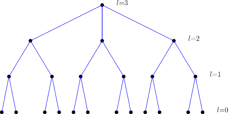
Figure 1: (Color online) A Cayley tree with with 4 levels ($l=0,1,2,3$) and coordination number $z=3$. Each node is connected to $z$ nearest neighbors except the nodes at the surface ($l=0$) which have only one neighbor. The deep interior of the tree where surface effects can be neglected is known as the Bethe lattice.

A Bethe lattice is an infinite-size branching tree of coordination number $z$. It may be visualized as the deep interior of a large branching tree (Cayley tree) of the same coordination number. Figure (1) shows a small ( 4 levels) Cayley tree with $z=3$ drawn such that the lattice points at the bottom row (level 0) are at the surface of the tree, and the point at the top (level 3) is at the root (center) of the tree. All lattice points except on the surface have $z$ nearest neighbors. A lattice point on the surface has only one neighbor. Analysis of hysteresis on a Cayley tree is simpler because there are no closed loops on the lattice. However most of the lattice points lie on the surface and therefore special care has to be exercised to ensure that the results apply to the deep interior of the tree and are insensitive to conditions on the surface. We adopt two separate methods to eliminate the surface effects. In our analytic calculations we use recursion relations that take us from the surface towards the interior of the tree level by level. Fixed-points of these recursion relations are insensitive to the random-fields on the surface. In numerical simulations we employ a different strategy. We perform simulations on a surfaceless random graph of coordination number $z$. The two methods of eliminating surface effects are equivalent and therefore our theoretical results match our simulation results perfectly.

Consider a tree whose sites are randomly occupied by an Ising spin with probability $c$. If $c$ is slightly less than unity the lattice acquires holes (regions without spins). For values of $c$ closer to zero it breaks up into disjointed clusters of spins. It is not immediately obvious that the earlier method of recursion relations  dhar starting from the surface of a compact lattice ($c=1$) and moving towards its interior is still useful i.e. if it would yield fixed-points in spite of enhanced surface effects. But we find that the method works over the entire range $0\leq c\leq 1$. We start with a diluted lattice and $h=-\infty$ so that all spins are down initially. The field is slowly ramped up from $-\infty$ to $h$ and we ask what fraction of spins are up at $h$. We choose a site at random in the deep interior of the tree and call it the central site. The probability that the central site is occupied by a spin is equal to $c$. We now calculate the probability that it is up as well. Each nearest neighbor of the central site if it is occupied by a spin forms the vertex of a subtree. The subtrees do not interact with each other except through the central site. Therefore the evolution on $z$ subtrees meeting at the central site is independent of each other as long as the central site does not flip up from its initial state. It is an important property of the model that the order in which the spins flip up does not influence the fixed-point at $h$  dhar , so we may assume that the central site is the last site to flip up at $h$ if it flips up at all. Before we can say whether the central sites may flip up or not, we need to know the conditional probability $cP^{*}(h)$ that a nearest neighbor of the central site is up given that the central site is down at applied field $h$.

$P^{*}(h)$ is the fixed point of the recursion equation,

$$P^{l}(h)=\sum_{i=0}^{z-1}\binom{z-1}{i}{(1-c)}^{i}\left[\sum_{j=0}^{z-1-i}\binom{z-1-i}{j}\left\{cP^{l-1}(h)\right\}^{j}\left\{c-cP^{l-1}(h)\right\}^{z-1-i-j}p_{j}(i;h)\right]$$ (5)

The above equation is written on the assumption that all spins in the system were down before being exposed to a field $h$. Spins on the surface had the first chance to flip up at $h$, then spins on level 1 and so on. In this process of organized relaxation, spins up to level $l-1$ have been relaxed and we are at the point of calculating the probability that a spin at level $l$ (say at site $x$) flips up while spins at level $l+1$ are still down. With this explanation, equation (5) is easily understood after various symbols are defined. $P^{l}(h)$ is the conditional probability that the spin at site $x$ at level $l$ is up given that its nearest neighbor at level $l+1$ is down. Similarly, $P^{l-1}(h)$ is the conditional probability that a site at level $l-1$ is up given that its nearest neighbor at level $l$ (site $x$) is down. The site $x$ has one neighbor at level $l+1$ and $z-1$ neighbors at level $l-1$. These neighbors can be occupied by spins with probability $c$ or unoccupied with probability $1-c$. The neighbors at level $l-1$, if occupied, could be up or down independently of each other; $p_{j}(i;h)$ is the probability that site $x$ has sufficient quenched field to flip up at $h$ if $j$ neighbors are up, $i$ neighbors are unoccupied by spins, and consequently $z-j-i$ neighbors are down.

$$p_{j}(i;h)=\int_{(z-2j-i)J-h}^{\infty}\phi(h_{i})dh_{i};\hskip 14.22636pt\phi(hi)=\frac{1}{\sqrt{2\pi\sigma^{2}}}e^{\frac{-hi^{2}}{2\sigma^{2}}}$$ (6)

The probability that a randomly chosen site on the lattice (the central site) is occupied and up is,

$$p(h)=c\sum_{i=0}^{z}\binom{z}{i}\{1-c\}^{i}\left[\sum_{j=0}^{z-i}\binom{z-i}{j}\{cP^{*}(h)\}^{j}\{c-cP^{*}(h)\}^{z-i-j}p_{j}(i,h)\right]$$ (7)

The magnetization per spin on the lower and upper half of the major hysteresis loop is given by

$$m^{*}_{l}(h)=2p(h)-c;\mbox{\hskip 14.22636pt}m^{*}_{u}(h)=-m^{*}_{l}(-h)$$ (8)

If we reverse the applied field before completing the lower half of the major loop, we generate a minor hysteresis loop. First reversal of the field generates the upper half of the minor loop, and a second reversal generates the lower half. When the field on second reversal reaches the point where the first reversal was made, the lower half of the minor loop meets the starting point of the upper half. In other words, the minor loop closes upon itself at the point where it started. This property of the random-field Ising model is known as the return point memory. Consider the upper half of the minor loop. Suppose the applied field is reversed from $h$ to $h^{d}$ $(h^{d}\leq h)$. We need to calculate the probability that an occupied site, say site $x$, that is up at $h$ turns down at $h^{d}$. When site $x$ turns up at $h$, the field on its nearest neighbors increases by an amount $2J$. This may cause some neighbors to turn up as well. Each neighbor that turns up increases the field on site $x$ by an amount $2J$. Therefore on reversing the field, site $x$ can turn down only after all neighbors which turned up after it have turned down. The probability $D^{*}(h^{d})$ that an occupied nearest neighbor of site $x$ that was down before site $x$ turned up at $h$ is again down at $h^{d}$ is determined by the fixed point of the following recursion relation.

$$\begin{split}D^{*}(h^{d})=c\sum_{i=0}^{z-1}\binom{z-1}{i}{(1-c)}^{i}\left[\sum_{j=0}^{z-1-i}\binom{z-1-i}{j}\{cP^{*}(h)\}^{j}\{c-cP^{*}(h)\}^{z-1-j-i}\{1-p_{j+1}(i;h)\}\right]\\ +c\sum_{i=0}^{z-1}\binom{z-1}{i}{(1-c)}^{i}\left[\sum_{j=0}^{z-1-i}\binom{z-1-i}{j}\{cP^{*}(h)\}^{j}\{D^{*}(h^{d})\}^{z-1-j-i}\{p_{j+1}(i;h)-p_{j+1}(i;h^{d})\}\right]\end{split}$$ (9)

Given an occupied site $x$ that is up at $h$, the first sum above gives the conditional probability that an occupied nearest neighbor of $x$ remains down at $h$ after site $x$ has turned up. The second sum takes into account the situation that the nearest neighbor in question turns up at $h$ after site $x$ turns up but turns down at $h^{d}$.

The fraction of occupied sites that turn down at $h^{d}$ is given by

$$q(h^{d})=c\sum_{i=0}^{z}\binom{z}{i}{(1-c)}^{i}\left[\sum_{j=0}^{z-i}\binom{z-i}{j}\{cP^{*}(h)\}^{j}\{D^{*}(h^{d})\}^{z-i-j}\{p_{j}(i,h)-p_{j}(i,h^{d})\}\right]$$ (10)

The magnetization on the upper return loop and in the range of the applied field $h-2J\leq h^{d}\leq h$ is given by

$$m(h^{d})=2\{p(h)-q(h^{d})\}-c$$ (11)

At $h^{d}=h-2J$, all occupied neighbors of the central site that flipped up because the central site flipped up at $h$ would flip down but the central site would stay up. If the applied field decreases further, the central site would turn down before any of its occupied nearest neighbors. This means that at $h-2J$ the system arrives at some point on the upper half of the major hysteresis loop, and moves on it upon further decrease in the applied field . The magnetization for $h^{d}\leq h-2J$ is given by

$$m(h^{d})=2\tilde{p}(h^{d})-c$$ (12)

Where,

$$\begin{split}\tilde{p}(h^{d})=c\sum_{i=0}^{z}\binom{z}{i}{(1-c)}^{i}\left[\sum_{j=0}^{z-i}\binom{z-i}{j}\{c\tilde{P}^{*}(h^{d})\}^{j}\{(1-c\tilde{P}^{*}(h^{d}))\}^{z-i-j}p_{j}(i;h^{d})\right]\end{split}$$ (13)

and $\tilde{P}^{*}(h^{d})$ is given by the fixed point of the following recursion relation.

$$\begin{split}\tilde{P}^{l}(h^{d})=\sum_{i=0}^{z-1}\binom{z-1}{i}{(1-c)}^{i}\left[\sum_{j=0}^{z-1-i}\binom{z-1-i}{j}\{c\tilde{P}^{l-1}(h^{d})\}^{j}\{c-c\tilde{P}^{l-1}(h^{d})\}^{z-1-i-j}p_{j+1}(i;h^{d})\right]\end{split}$$ (14)

The lower half of the return loop is obtained by reversing the field from $h^{d}$′ to $h^{u}$ ($h^{u}>h^{d}$). If $h^{d}′<h-2J$, the lower half of the minor loop starts from the major loop, and therefore it is related by symmetry to the upper half of the return loop that has been obtained above. We only need to consider the case $h^{d}\geq h-2J$. In this case, the magnetization on the lower half of the return loop may be written as,

$$m(h^{u})=2\{p(h)-q(h^{d})+p^{\prime}(h^{u})\}-c$$ (15)

Where $p^{\prime}(h^{u})$ is the probability that an occupied site that is up at $h$, down at $h^{d}$, turns up again at $h^{u}$.

$$p^{\prime}(h^{u})=c\sum_{i=0}^{z}\binom{z}{i}{(1-c)}^{i}\left[\sum_{j=0}^{z-i}\binom{z-i}{j}\{U^{*}(h^{u})\}^{j}\{D^{*}(h^{d})\}^{z-i-j}\{p_{j}(i,h^{u})-p_{j}(i,h^{d})\}\right]$$ (16)

Here $U^{*}(h^{u})$ is the conditional probability that an occupied nearest neighbor of a site $x$ turns up before site $x$ turns up on the lower return loop. It is determined by the fixed point of the following equation.

$$\begin{split}U^{*}(h^{u})=cP^{*}(h)-c\sum_{i=0}^{z-1}\binom{z-1}{i}{(1-c)}^{i}\left[\sum_{j=0}^{z-1-j}\binom{z-1-i}{j}\{cP^{*}(h)\}^{j}\{D^{*}(h^{d})\}^{z-1-i-j}\{p_{j}(i,h)-p_{j}(i,h^{d})\}\right]\\ +c\sum_{i=0}^{z-1}\binom{z-1}{i}{(1-c)}^{i}\left[\sum_{j=0}^{z-1-i}\binom{z-1-i}{j}\{U^{*}(h^{u})\}^{j}\{D^{*}(h^{d})\}^{z-1-i-j}\{p_{j}(i,h^{u})-p_{j}(i,h^{d})\}\right]\end{split}$$ (17)

The rationale for the equation (17) is as follows. Given an occupied site $x$ that is down at $h^{d}$, the first two terms on the right hand side account for the probability that an occupied nearest neighbor of site $x$ is up at $h^{u}\geq h^{d}$. Note that the neighbor in question must have been up at h in order to be up at $h^{d}$, and if it is already up at $h^{d}$, then it will remain up on the entire lower half of the return loop, i.e. at $h^{u}\geq h^{d}$. The last term gives the probability that the nearest neighbor was down at $h^{d}$, but turned up on the lower return loop before site $x$ turned up. It can be verified that the lower return loop meets the lower major loop at $h^{u}=h$ and merges with it for $h^{u}>h$, thus proving the property of return point memory.

The method of calculating the minor loop may be extended to obtain a series of smaller minor loops nested within the minor loop obtained above. The key point is that whenever the applied field is reversed, a site $x$ may flip only after all neighbors of site $x$ which flipped in response to the flipping of site $x$ on the immediately preceding sector have flipped back. The neighbors of site $x$ which did not flip on the preceding sector in response to the flipping of site $x$ do not flip in the reversed field before site $x$ has flipped. We have obtained above expression for the return loop when the applied field is reversed from $h$ on the lower major loop to $h^{d}$′ ($h-2J\leq h^{d}′\leq h$), and reversed again from $h^{d}$′ to $h^{u}$′′ ($h^{u}′\leq h$). When the applied field is reversed a third time from $h^{u}$ to $h^{dd}$ ($h^{dd}<h^{u}$), expressions for the magnetization on the nested return loop follow the same structure as the one on the trajectory from $h$ to $h^{d}$.

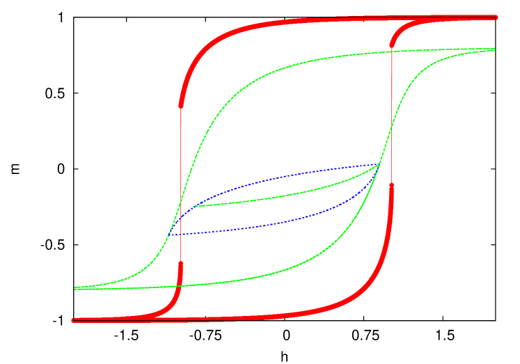
Figure 2: (Color online) Hysteresis loops on a $z=4$ lattice for $\sigma=1.7$: The larger loop (red/dark) with saturation at $m=\pm 1$ and first-order jumps in the magnetization is for $c=1$ (undiluted lattice); the smaller loop (green/grey) with saturation at $m=\pm 0.8$ is for $c=0.8$; Two minor loops within the smaller loop are also shown which are obtained by making excursions from $h=0.9$ to $h=-1.1$ and $h=-0.85$ respectively.

The analytic results obtained above are depicted in Figure (2) for $\sigma=1.7$ and $z=4$ for two concentrations of magnetic minerals; (i) c=1 (no dilution), and (ii) c=0.8 . The fixed point of equation (5) is evaluated numerically for a sufficiently large and negative applied field $h$, and used in equations (7) and (8) to obtain the magnetization at the start of the lower half of the hysteresis loop ($m_{l}^{*}\approx-c$). The applied field $h$ is then increased in small steps, and the process is repeated to determine $m_{l}^{*}(h)$ along the lower half of the hysteresis loop. Similarly, minor loops are obtained using equations (9) to (17). The upper half of the hysteresis loop is obtained by the relation $m_{u}^{*}(h)=-m_{l}^{*}(-h)$. Hysteresis on a $z\geq 4$ lattice is qualitatively different from the case of $z=2$ and $z=3$. For $z\geq 4$ there exists a non-equilibrium critical point ($\sigma=\sigma_{c},h=h_{c}$) on the lower half of the hysteresis loop, and another symmetrically placed critical point on the upper half. At these non-equilibrium critical points the response of the system to a slowly varying driving field is singular. Critical points do not exist on lattices with $z=2,3$. Let us focus on the critical point on the lower half of the hysteresis loop. For $z=4$ and $c=1$, we have $\sigma_{c}\approx 1.78$. For $z>4$, $\sigma_{c}$ increases with increasing $z$. For $\sigma<\sigma_{c}$, the two halves of the hysteresis loop have first order jumps in the magnetization as shown in Figure (2). For $c<1$, there is extra disorder in the system on account of the dilution of magnetic sites. This causes the first order jumps at $\sigma=1.78$ for $c=1$ to vanish at $c=0.8$, and the major hysteresis loop becomes smooth as seen in Figure (2). We have also shown two minor hysteresis loops for $c=0.8$. If $c<1$ but sufficiently large to form spanning clusters of occupied sites on the lattice, the qualitative behavior of hysteresis is similar to that on the undiluted lattice with $c=1$ but with an effectively reduced value of $\sigma_{c}$. These results are verified by numerical simulations of the model for the corresponding choices of the parameters $z,J,c$, and $\sigma$. As stated earlier, we performed numerical simulations on random graphs to eliminate surface effects. A random graph of N sites has no surface, but the price we pay is that it has some loops. However, for almost all sites in the graph, the local connectivity up to a distance of $log_{(z-1)}N$ is similar to the one in the deep interior of the branching tree. Thus the the theoretical results depicted in Figure (2) to (4) perfectly matched the corresponding results from the simulations of the model on random graphs. Indeed, the theoretical and simulation results are indistinguishable on the scale of the figures.

IV Application to rock magnetism

There are a variety of models in the literature that explain the shape of hysteresis loops in magnetic rock samples. Our objective is not merely to add to this list of models but also to simplify the situation. Our point is that extant models of ferromagnetic hysteresis also explain hysteresis in magnetic rocks if we add the ingredient of dilution to them. We have chosen the random field Ising model of hysteresis in ferromagnets at zero temperature and in the limit of zero frequency of the driving field. The advantage of this model is that it can be solved exactly on a Bethe lattice of an arbitrary coordination number $z$ shukla . The model has only a few parameters; the coordination number $z$ of the lattice, the interaction energy $J$ that aligns nearest neighbor spins parallel to each other, and a parameter $\sigma$ that tends to disorder the system. In spite of its simplicity, this model explains a number of experimental observations regarding return point memory, Barkhausen noise, non-equilibrium critical points on hysteresis loops, and universal behavior in the vicinity of these points sethna1 ; sethna2 . All we have done is diluted this model, i.e. only a fraction $c$ of the sites are occupied by magnetic entities. We have solved the dilute model exactly. Drawing upon the empirical observation that the magnetic minerals in a rock account for only a few percent of its mass, one may ask if the predicted hysteretic behavior of our model in the range $0.01\leq c\leq 0.1$ is reasonably close to the observed behavior of magnetic rocks. It indeed appears to be the case considering the minimal number of free parameters in our model.

Figure (3) shows three hysteresis loops for $c=0.1$; and $\sigma=0.05,0.2$, and $0.5$ respectively. We have set $J=1$ for convenience. Let us focus on $\sigma=0.05$ first. As the applied field $h$ increases from $h=-\infty$ the magnetization stays at its saturation value $m=-0.1$ until $h\approx-3\sigma$. It rises sharply from $m\approx-0.1$ to $m\approx 0.03$ around $h\approx 0$, and from $m\approx 0.03$ to $m\approx 0.1$ around $h\approx 1$. The rise around $h=0$ is due to isolated spins in the system. The quenched field has a Gaussian distribution with average value zero and standard deviation $\sigma$. Therefore some of the isolated sites turn up at $h\approx-3\sigma$, and almost all of them are up at $h\approx 3\sigma$. The fraction of isolated sites is $c(1-c)^{4}$. This is approximately equal to $0.034$. Occupied sites in clusters of size larger than unity account for the remaining fraction $0.066$. After all isolated sites have turned up the magnetization per site increases to $-0.1+2\times 0.34=.032$. It stays at this plateau value until the applied field increases further by an amount $2J-3\sigma$ enabling some surface sites of a connected cluster of down spins (dangling bonds) to turn up. Nearly all sites turn up at $h=2J+3\sigma$ and we get the saturated magnetization $m=.1$ as shown in figure (3). The same mechanism applies to hysteresis loops for other values of $\sigma$. With increasing $\sigma$ the sharp corners tend to get more rounded and the middle (pinched) portion of the loop broadens. We get a gentle pinched loop for $\sigma=0.2$. For $\sigma=0.5$ the constriction in the middle disappears completely and we get a normal ferromagnetic type of hysteresis loop as shown in figure (3). Thus our model reproduces various shapes of hysteresis loops observed in magnetic rocks with a minimum number of parameters and without invoking different mechanisms for different shapes. Figure 4 (see caption) shows another way of representing the same data as shown in figure 3. In this representation, the constriction in the middle of the hysteresis loop appears as a more pronounced dip in the middle of the plot and therefore it may be of some value in the analysis of experimental data.

Can we deduce the magnetic composition of the rock from the shape of its hysteresis loop? This is not possible in general because the hysteresis loop contains the information in an integrated form. Information is irreversibly lost in the process of integration and can not be retrieved. There is no unique way to obtain the components of a sum from the sum! However, our model provides a few guiding principles. Ferromagnetic shapes of hysteresis loops indicate a larger random-field disorder $\sigma$ in the system. On the other hand a wasp-waisted loop especially with a long and narrow waist and sharp bends indicates relatively small disorder $\sigma$. In this case the connectivity of spins at the surface of clusters has the larger effect on the shape of hysteresis loops. It should be possible to deduce the magnitude of interaction $J$ from the locations of sharp turns in the magnetization along the applied field. Similarly, it should be possible to deduce the relative size of clusters from the plateaus in the magnetization. The distribution of cluster sizes and the plateaus of the magnetizations are known exactly in our model in terms of the two parameters ($J$ and $\sigma$) of the model. However, more complex rock samples may not be adequately characterized by a simple two-parameter Hamiltonian. Also, there may be systems whose frozen disorder is not represented adequately by a Gaussian distribution. We have focused on the Gaussian distribution because it applies to many systems  sethna1 ; sethna2 and its use is justified by the central limit theorem. The effect of the shape of random-field distribution on critical hysteresis in the random-field Ising model ($c=1$) has been examined by Liu and Dahmen liu . They find that the Lorentzian and parabolic distributions of random fields yield the same critical exponents in three dimensions as the Gaussian random fields. This is not entirely surprising because a renormalization group analysis in $6-\epsilon$ dimensions  dahmen shows that for random-field distributions with a single maximum, it is only the curvature of the distribution at its maximum that determines the critical exponents. Therefore it is reasonable to use the Gaussian distribution as a common representative of smooth single-peaked distributions which all give the same critical exponents that agree with experiments. In the same vein, we have used the Gaussian distribution to understand the shapes of hysteresis loops in the strongly diluted limit of the random-field model. Before ending, we also wish to mention that wasp-waisted loops are not a property of magnetic rock samples only. Such loops are also seen in random magnets with the order parameter having a continuous symmetry shukla2 , shape memory alloys straka ; murray , and martensites goicoechea . Indeed the physics behind hysteresis in the random field Blume-Emery-Griffiths model goicoechea is very similar to that discussed here in the case of the dilute random-field Ising model.

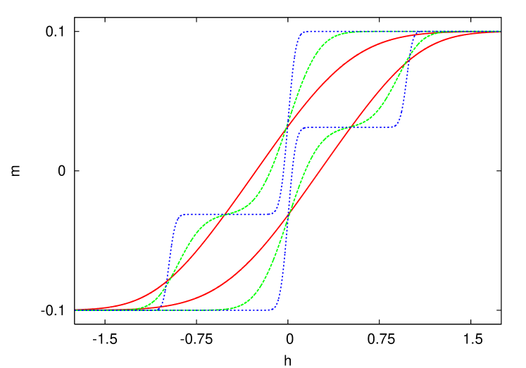
Figure 3: (Color online) Hysteresis loops on a lattice with $z=4$ and $c=0.1$ as may be appropriate for magnetic rock samples. The saturation $m=\pm 0.1$ is controlled by the fractional content of magnetic minerals in the rock ($c=0.1$) but the shapes depend on $\sigma$. Three representative cases are shown: (i) ferromagnetic shape shown in red (loop with the largest width at $m=0$ for $\sigma=0.5$; (ii) a very pronounced wasp-waisted loop in blue (loop with the smallest width at $m=0$) for $\sigma=0.05$, and (iii) a wasp-waisted loop in green (having intermediate width at $m=0$ for $\sigma=0.2$).

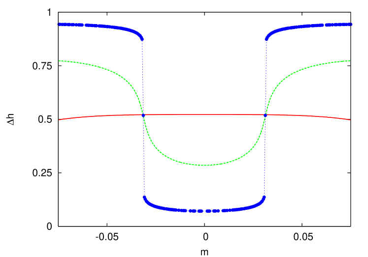
Figure 4: (Color online) This is a different representation of figure (3). For a fixed magnetization $m$ along the $x$-axis, the $y$-axis shows the difference of corresponding applied fields on the upper and lower halves of the hysteresis loop. The red line (nearly horizontal thin line) corresponds to $\sigma=.5$, the blue line (thick line with two nearly vertical jumps) corresponds to $\sigma=0.05$. The green line (intermediate dotted line) corresponds to $\sigma=0.2$.

References

- (1) See, for example, The Science of Hysteresis, edited by G Bertotti and I Mayergoyz, (Academic Press, Amsterdam, 2006).
- (2) J P Sethna, K Dahmen, S Kartha, J A Krumhansl, B W Roberts, and J D Shore, Phys Rev Lett 70, 3347 (1993).
- (3) J P Sethna, K Dahmen, O Perkovic. The Science of Hysteresis (Elsevier Inc 2005) Vol 2. Ch 2. pp 107-179.
- (4) Y Imry and S -k Ma, Phys Rev Lett 35, 1399 (1975).
- (5) D P Belanger and T Nattermann, in Spin Glasses and Random Fields edited by A P Young ( World Scientific, Singapore, 1998 ).
- (6) J Villain, Phys Rev Lett 52, 1543 (1984); G Grinstein and J F Fernandez, Phys Rev B 29, 6389 (1984); A J Bray and M A Moore, J Phys C 18, L 927 (1985).
- (7) D S Fisher, Phys Rev Lett 56, 416 (1986).
- (8) J P Sethna, K A Dahmen, and C R Myers, Nature (London) 410, 242 (2001) and references therein.
- (9) D Dhar, P Shukla, J P Sethna, J Phys A30, 5259 (1997).
- (10) P Shukla, Prog Theo Phys, Vol 96, No 1 (1996); P Shukla, Physica A 233,235 (1996); P Shukla,Phys Rev E 62, 4725 (2000); P Shukla,Phys Rev E 63,027102 (2001).
- (11) P Shukla and R S Kharwanlang, Phys Rev E 81, 031106 (2010); P Shukla and R S Kharwanlang, Phys Rev E 83, 011121 (2011).
- (12) Rock Magnetism: Fundamentals and Frontiers by D J Dunlop and O Ozdemir, Cambridge University Press, 2001.
- (13) D J Dunlop. Physics of the Earth and Planetary Interiors 26, 1-26 (1981).
- (14) An important aspect of rock magnetism (not discussed here) is that it provides a recorded memory of the intensity, direction, and polarity of the Earth’s magnetic field in the geological past. It reveals that the polarity of Earth’s magnetic field has reversed several times in the past, most recently about 780,000 years ago. This discovery revolutionized the field in the 1960s by providing evidence for continental drift and plate tectonics. See for example, D J Dunlop, ”Rock magnetism” in AccessScience, @McGraw-Hill Companies, 2008,http://www.accessscience.com
- (15) A P Roberts, Y Cui, K L Verosub. J Geo Phys Res 100, 17909-17924 (1995), and references therein.
- (16) A P Roberts, C R Pike, K L Verosub. J Geo Phys Res 105, 28461-28475 (2000).
- (17) L Tauxe, T A T Mullender, T Pick. J Geo Phys Res 101, 571-583 (1996).
- (18) P J Wasilewski, Earth Planet Sci Lett 20, 67-72 (1973).
- (19) J J Becker. IEEE Trans Magn Mag 18,1451-1453 (1982).
- (20) T Pick, L Tauxe. J Geo Phys Res 98,17949-17964 (1993).
- (21) T Pick, L Tauxe. Geo Phys J Int 119, 116-128 (1994); E502 (2005).
- (22) C P Bean, J Appl Phys 26,11 (1955).
- (23) P Hejda, A Kapicka, E Petrovsky, B A Sjoberg. IEEE Trans Magn 30,2 (1994).
- (24) L H Bennett and E D Torre. J Appl Phys 97 10E502 (2005).
- (25) J E Davies, L H Bennett, E D Torre, B C Choi, S N Piramanayagam, and E Girgis, IEEE Transactions on Magnetics, vol 44, 2722-2725 (2008).
- (26) L Tauxe, H N Bertram, and C Seberino, Geochem. Geophys. Geosyst., 3 (10), 1055 (2002). doi:10.1029/2001GC000241
- (27) G Kletetschka, and P J Wasilewski, Physics of the Earth and Planetary Interiors 129, 173-179 (2002).
- (28) Y Liu and K A Dahmen, Phys Rev E 79, 061124 (2009).
- (29) K Dahmen and J P Sethna, Phys Rev B 53, 14872 (1996).
- (30) L Straka, O Heczko, and N Lanska, IEEE Trans Magn 38, 5 (2002)
- (31) S J Murray, M Marioni, S M Allen, R C O’Handley, and T A Lograsso, Appll Phys Lett 77, 6 (2000)
- (32) J Goicoechea and J Ortin, J Phys IV France 05, C2-71 (1995).