AC susceptibility investigation of vortex dynamics
in nearly-optimally doped REFeAsO_1-xF_x superconductors (RE = La, Ce, Sm)

Abstract

Ac susceptibility and static magnetization measurements were performed in the nearly-optimally doped LaFeAsO_0.9F_0.1 and CeFeAsO_0.92F_0.08 superconductors, complementing earlier results on SmFeAsO_0.8F_0.2 [Phys. Rev. B 83, 174514 (2011)]. The magnetic field – temperature phase diagram of the mixed superconducting state is drawn for the three materials, displaying a sizeable reduction of the liquid phase upon increasing $T_{c}$ in the range of applied fields ($H\leq 5$ T). This result indicates that SmFeAsO_0.8F_0.2 is the most interesting compound among the investigated ones in view of possible applications. The field-dependence of the intra-grain depinning energy $U_{0}$ exhibits a common trend for all the samples with a typical crossover field value ($2500$ Oe $\lesssim H_{cr}\lesssim 5000$ Oe) separating regions where single and collective depinning processes are at work. Analysis of the data in terms of a simple two-fluid picture for slightly anisotropic materials allows to estimate the zero-temperature penetration depth $\lambda_{ab}(0)$ and the anisotropy parameter $\gamma$ for the three materials. Finally, a sizeable suppression of the superfluid density is deduced in a $s^{\pm}$ two-gap scenario.

I Introduction

Almost four years after the discovery of high-temperature superconductivity in Fe-based pnictides,Kam08 several questions are still open both on fundamental aspects and on possible technological applications. No clear and exhaustive explanations for the precise pairing mechanism have been given yet. Incontrovertible features of isotopic effects cannot entirely rule out a partial role of the lattice in the coupling process,Liu09 but it is essential to stress that $T_{c}$’s values are indeed too high to allow only a conventional pairing to be at work.Boe08 Strong evidences for a multi-band $s^{\pm}$ scenario similar to that proposed for magnesium di-borideGon02 have been reported, together with theoretical support,Bus10 ; Umm11 from a number of techniques in materials belonging to the 1111 family,Hun08 ; Dag09 ; Lee09 ; Wey10 to 122 compoundsKha09 and to 11 chalcogenides.Kha10

At the same time, it is still not clear whether these novel compounds will be helpful as valid technological tools. The answer to these problems will essentially come from specific measurements of critical current densities in relation to the features of the grain boundaries. Detailed studies of the practical applicability of granular superconductors, anyway, cannot leave aside precise investigations of the fundamental intrinsic properties of the materials. In this respect, the determination of the so-called irreversibility line is of the utmost importance. Such line, in fact, delimits the region in the magnetic field - temperature phase diagram where the dissipationless property of the thermodynamical superconducting phase is preserved even in the presence of a partial penetration of magnetic field inside the material. In a previous work on a powder sample of optimally-doped SmFeAsO_0.8F_0.2 (see Ref. Pra11, ) the determination of the intrinsic irreversibility line was performed by means of the ac susceptibility technique. Parameters like the superconducting critical temperature $T_{c}$ are anyway well known to be strongly dependent on the considered RE ion.Joh10 The question of whether (and how) the properties of the phase diagram of the flux lines and of the relative irreversibility lines too are indeed dependent on the RE ion is then of extreme importance.

In this paper we report on the phase diagram of the flux lines in three powder samples of REFeAsO_1-xF_x superconductors (RE = La, Ce, Sm) under conditions of nearly-optimal doping. In particular, much attention is devoted to the determination of the irreversibility line and its dependence on the RE ion. The features of pinning mechanisms and, in particular, of the characteristic depinning energy barriers are investigated in detail within a thermally-activated framework. Results are interpreted and analyzed by distinguishing two magnetic field regimes characterized by single and collective depinning processes. Together with a simple two-fluid model and a proper normalization, this allows us to make experimental data collapse on the same curve, a feature indicative of a common underlying mechanism independent on the precise material. Reliable estimates of the zero-temperature penetration depth $\lambda_{ab}(0)$ and of the dependence of the anisotropy parameter $\gamma$ on the RE ion are finally given, together with some interpretations of the observed behaviour in terms of a two-band $s^{\pm}$ model. Data relative to the Sm-based sample have already been presented in Ref. Pra11, and will be reported also here for the sake of clarity and completeness.

II Experimentals. Aspects of DC magnetization and AC susceptibility

Powder samples of REFeAsO_1-xF_x (with RE = La, Ce, Sm and nominal F^- contents $x=0.1$, $0.08$ and $0.2$, respectively) were synthesized as described in previous works.Pra11 ; Pra11b ; Kon09 ; Zhu08 Static magnetization $M_{dc}$ and ac susceptibility $\chi_{ac}$ measurements were performed by means of a Quantum Design MPMS-XL7 SQUID magnetometer and of a MPMS-XL5 SQUID susceptometer, respectively. In the latter case a small alternating magnetic field $H_{ac}$ with frequency $\nu_{m}$ is superimposed to a much higher static magnetic field $H$. Measurements were always performed in field-cooled (FC) conditions with $H_{ac}=0.0675-1.5$ Oe parallel to $\mu_{0}H$, which varied up to 5 T, while $\nu_{m}$ ranged from $37$ to $1488$ Hz.

$M_{dc}/H$ vs. temperature ($T$) raw data obtained under FC conditions at $H=5$ Oe are shown in Fig. 1. For the sake of clarity the curves have been reported after subtracting slight spurious contributions, leaving data above the superconducting onset at a constant zero offset value. $T_{c}(0)$ is defined as the critical temperature $T_{c}$ for $H\rightarrow 0$ Oe. Such values are obtained as the zero intercept of a linear extrapolation of data below the diamagnetic onsetPra11 and reported in Fig. 1 in correspondence of the diamagnetic onsets of the three samples. The saturation absolute value of the diamagnetic signals can be evaluated around $\left(0.27\pm 0.05\right)$ in $1/4\pi$ units. These values are typical for fully-superconducting powder samples in measurements under FC conditions, the observed reduction originating from the sample’s geometrical properties and morphology. In the case of the CeFeAsO_0.92F_0.08 sample, a sizeable paramagnetic contribution from the Ce sublattice can be clearly discerned already at such low value of magnetic field, mainly due to the high value of the Ce³⁺ magnetic moment. In fact, the fitting procedure to the experimental data at several values of $H$ already described in a previous workPra11 yields to $\mu_{Ce}\simeq 2.1\;\mu_{B}$ and $\mu_{Sm}\simeq 0.3\;\mu_{B}$ (raw data not shown).

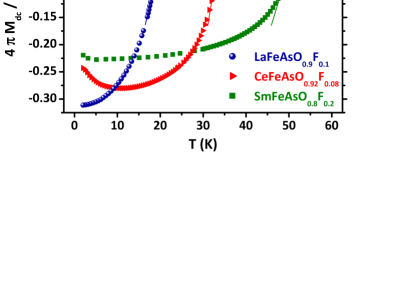
Figure 1: (Color online) $M_{dc}/H$ vs. $T$ curves (volume units) in FC conditions at $H=5$ Oe. The estimated $T_{c}(0)$ values are indicated in correspondence of the diamagnetic onsets.

Curves reported in Fig. 1 show quite sharp superconducting transitions. The slight roundness of the onset may be due to several reasons, both intrinsic (for instance the influence of superconducting fluctuations near $T_{c}$, as already discussed in Ref. Pra11b, ) and extrinsic (slight chemical inhomogeneity of the F^- doping ions, distribution of the geometrical size of grains). The signal, moreover, comes from differently oriented grains in the powder sample and also this fact may contribute to a broadening of the transition. The corresponding powder-averaged upper critical field

$$\langle H_{c2}(T)\rangle_{pwd}\simeq\frac{2}{3}H_{c2,H\parallel ab}(T)+\frac{1}{3}H_{c2,H\parallel c}(T)$$ (1)

was deduced for the three samples by examining the field dependence of $T_{c}$, as reported in Ref. Pra11, .

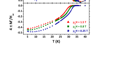
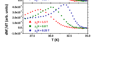
Figure 2: (Color online) Left: $\chi_{ac}$ vs. $T$ raw data for CeFeAsO_0.92F_0.08 ($H_{ac}=1.5$ Oe and $\nu_{m}=478$ Hz) at different $H$ values. The imaginary and the real components are shown in the upper and lower panels, respectively (volume units). Right: zoom of the onset region of the curves already reported in the left panels relative to $\chi_{ac}^{\prime\prime}$ and to the first derivative of $\chi_{ac}^{\prime}$ with respect to $T$ (upper and lower panels, respectively. See text for further details).

In Fig. 2 some typical $\chi_{ac}$ vs. $T$ curves for CeFeAsO_0.92F_0.08 are displayed (raw data of SmFeAsO_0.8F_0.2 have been reported previouslyPra11 ). Raw data for LaFeAsO_0.9F_0.1 are qualitatively similar to those in Fig. 2 and are not presented. The $\chi_{ac}^{\prime}$ vs. $T$ curves can be described in terms of a mixed-state shielding response with some degree of distortion occurring in those $T$ regions where sizeable contributions to the imaginary component appear. $\chi_{ac}^{\prime\prime}$ vs. $T$ curves are composed of two main peaked contributions: a narrow peak appears just below the diamagnetic onset while a much broader one is present at low $T$. This is quite a common phenomenology in superconducting powder samples.Nik89 ; Gom97 The high-$T$ peak is generally associated with the power absorption due to losses inside the single grains, while the broad low-$T$ peak can be associated with the generation of weak Josephson-like links among the different grains.

The three main features shown in Fig. 2, namely the diamagnetic onset in $\chi_{ac}^{\prime}$ and the two peaks in $\chi_{ac}^{\prime\prime}$, are strongly shifted to lower $T$ on increasing $H$ for all the samples. The $H$-dependence of the diamagnetic onset in $\chi_{ac}^{\prime}$, in particular, is much more marked than in the case of the diamagnetic onset in $M_{dc}/H$ vs. $T$ curves. The described behaviour can be directly associated to vortex dynamics and to the precise features of the irreversibility line.Pra11 ; Mal88 ; Tin88 ; VdB91 ; VdB93 ; Zhe94 When dealing with an electromagnetic wave impinging on a type II superconducting material, in fact, one has to carefully take into consideration typical spatial penetration lengthscales. The general treatment of the problem has been considered in several papers.Bra91 ; Cof92 ; Pro03 ; Pro11 In the presence of vortices, in particular, the overall penetration depth $\lambda_{ac}$ for the radiation can be generally expressed as the quadrature sum of $\lambda_{L}$ (representing the London penetration depth of the superconductor) and $\lambda_{C}$ (the so-called Campbell penetration depth), namely

$$\lambda_{ac}=\sqrt{\lambda_{L}^{2}+\lambda_{C}^{2}}.$$ (2)

$\lambda_{C}$ can be generally expressed asPro11

$$\lambda_{C}=\sqrt{\frac{\Phi_{0}H}{4\pi\alpha}}$$ (3)

where the Labusch parameter $\alpha$ mimics the curvature of the potential well associated with the pinning centers in a harmonic approximation. In other terms, $\alpha$ quantifies the average elastic restoring force density of the pinning centers acting on the flux lines (FLs).

The case of high effectiveness of the pinning mechanisms ($\alpha\rightarrow\infty$) ideally corresponds to a condition where FLs are completely fixed. This condition is, by definition, the so-called glassy phase of FLs where typically irreversible processes develop.Yes96 By qualitatively considering Eqs. (2) and (3) under these circumstancies, one notices that the penetration of the electromagnetic wave is only governed by the London penetration depth $\left(\lambda_{ac}\rightarrow\lambda_{L}\right)$. As a result, the electromagnetic wave is shielded by the superconductor leading to a diamagnetic response in $\chi_{ac}^{\prime}$. On the other hand, in the opposite case of completely ineffective pinning the Labusch constant can be considered as a vanishing quantity. In this case, the FLs are in the so-called liquid state and are substantially free to move generating dissipation. The condition $\alpha\rightarrow 0$ yields to $\lambda_{C}\rightarrow\infty$ or, at least, to $\lambda_{C}\gg R$ in the case of a powder sample ($R$ is the typical grain size) and no shielding can be detected even in the presence of a robust thermodynamical superconducting phase. As a result, $\chi_{ac}^{\prime}=0$ even if $M_{dc}/H$ already takes negative diamagnetic values. The onset of the diamagnetic response of the material in $\chi_{ac}^{\prime}$ vs. $T$ curves can then be interpreted as a crossover between the two described phases of the FLs and its $H$-dependence is a good choice in order to define the irreversibility line.

A slightly different criterion for determining the irreversibility line can be formulated by considering the intrinsic dissipative response inside the grains.Pra11 ; VdB91 ; Pal90 ; Emm91 ; Tin91 In particular, by now considering the $\chi_{ac}^{\prime\prime}$ vs. $T$ curves, one can denote by $T_{p}$ the position of the intra-grain maximum which is typically found just few-K below the diamagnetic onset in $\chi_{ac}^{\prime}$. This peak can be interpreted as arising from a resonating absorption of energy when the frequency of the radiation matches the inverse characteristic relaxation time $1/\tau_{c}$ of the vortices in the pinning potential dip, namely

$$2\pi\nu_{m}\tau_{c}|_{{}_{T=T_{p}}}=1.$$ (4)

The $H$-dependence of $T_{p}$ can then be chosen in order to describe the irreversibility line and in the following we will be referring to this as the $\chi_{ac}^{\prime\prime}$-criterion. Within a Debye-like relaxation framework, $T_{p}$ almost coincides with the characteristic temperature of the corresponding peak in the derivative of $\chi_{ac}^{\prime}$ with respect to $T$. This was experimentally verified in all the three investigated samples,Pra11 as explicitly shown only in the case of CeFeAsO_0.92F_0.08 in the right panel of Fig. 2.

III Phase diagrams and depinning energy barriers: main results

The FLs phase diagrams for the three examined samples are shown in Fig. 3 where both $\langle H_{c2}(T)\rangle_{pwd}$ (full symbols) and the irreversibility lines (opened symbols) are plotted as a function of the reduced temperature $t\equiv T/T_{c}(0)$.

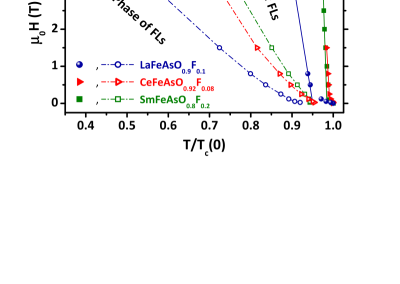
Figure 3: (Color online) Phase diagrams for the FLs in the investigated samples. Data for SmFeAsO_0.8F_0.2 have already been reported in Ref. Pra11, . Open symbols track the irreversibility line as deduced from data taken at $\nu_{m}=37$ Hz (dashed-dotted lines are guides for the eye). Full symbols track $\langle H_{c2}(T)\rangle_{pwd}$ (continuous lines are linear fits).

Table 1: Critical temperature $T_{c}(0)$ for $H\rightarrow 0$ Oe and correlation length $\langle\xi(0)\rangle_{pwd}$ for $T\rightarrow 0$ K as deduced from Eqs. (5) and (6).

Sample	$T_{c}(0)$ (K)	$\langle\xi(0)\rangle_{pwd}$ (Å)
SmFeAsO0.8F0.2	$52.3\pm 0.25$	$11.0\pm 0.1$
CeFeAsO0.92F0.08	$34.25\pm 0.25$	$15.7\pm 0.3$
LaFeAsO0.9F0.1	$20.2\pm 0.25$	$26.3\pm 0.5$

$\langle H_{c2}(T)\rangle_{pwd}$ vs. $t$ curves as determined from $M_{dc}$ data clearly display linear trends as a function of $t$. At low-$t$ values, anyway, a slight upper curvature can be detected for all the samples, a feature possibly associated with two-band superconductivity.Gur03 Data relative to CeFeAsO_0.92F_0.08 are limited to the low-$H$ values due to the dominant paramagnetic contribution arising from the Ce³⁺ sublattice which fully covers the superconducting response for $\mu_{0}H\gtrsim 2$ T. The slope of a linear fit to the data allows to estimate the upper critical field $\langle H_{c2}(0)\rangle_{pwd}$ extrapolated at $T=0$ K under the simplified assumption of single-band superconductivity through the Werthamer, Helfand and Hohenberg (WHH) relationWer66

$$\langle H_{c2}(0)\rangle_{pwd}\simeq 0.7\times T_{c}(0)\left|\frac{d\langle H_{c2}\rangle_{pwd}}{dT}\right|_{T\simeq T_{c}(0)}.$$ (5)

An overall correlation is observed between the gradual increase of $T_{c}(0)$ and a corresponding increase in the slope value and, accordingly, in the extrapolated $\langle H_{c2}(0)\rangle_{pwd}$. This, in turn, leads to a steady decrease of the extrapolated value of the powder-averaged Ginzburg-Landau (GL) coherence length $\langle\xi(0)\rangle_{pwd}$ at $T=0$ K, calculated from the relationTin96 ; DeG99 (see Tab. 1)

$$\langle H_{c2}(0)\rangle_{pwd}\equiv\frac{\Phi_{0}}{2\pi\langle\xi(0)\rangle_{pwd}^{2}}.$$ (6)

Results from $\chi_{ac}$ data will now be considered. The $\chi_{ac}^{\prime\prime}$-criterion was chosen for the determination of the irreversibility line. Data relative to the derivative of $\chi_{ac}^{\prime}$ were always analyzed due to their more favourable signal-to-noise ratio. A dependence of the $T_{p}$ value on $\nu_{m}$ was detected at all the values of the applied $H$. For this reason, data for the lowest accessible value $\nu_{m}=37$ Hz were chosen in order to draw the irreversibility lines in Fig. 3. It is possible to observe that the extension of the liquid phase of the flux lines is progressively reduced by the increase of $T_{c}$ in the explored $H$ range. This observation makes Sm-based materials rather interesting in view of possible technological applications.

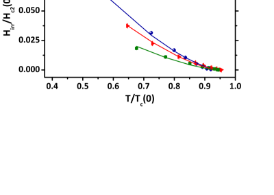
Figure 4: (Color online) Representation of the irreversibility lines relative to the investigated samples (already reported in the phase diagrams, see Fig. 3) where $H_{irr}(T)$ has been normalized with respect to the relative value of $\langle H_{c2}(0)\rangle_{pwd}$. Continuous lines are best-fits according to Eq. (7).

In order to better compare the behaviour of the three samples from a fundamental point of view, the irreversibility lines reported in Fig. 3 are presented again in Fig. 4 after normalizing the field values by $\langle H_{c2}(0)\rangle_{pwd}$. In all the three samples the irreversibility line can be described by means of a power-law function

$$\frac{H}{\langle H_{c2}(0)\rangle_{pwd}}\propto\left[0.95-\frac{T}{T_{c}(0)}\right]^{3/2}$$ (7)

characterized by the exponent $\beta=3/2$ (see the continuous lines in Fig. 4). This is a typical result in high-$T_{c}$ superconductors,Pra11 ; Mal88 ; Yes88 even if slightly different functional form have been reported, for instance, in the case of Ba(Fe_1-xCo_x)₂As₂ single-crystals.Pro08 Here the value $0.95$ (common for all the samples) phenomenologically accounts for the discrepancies at low magnetic fields when defining the irreversibility line from the $\chi_{ac}^{\prime\prime}$-criterion. It should be noticed that, when plotted on this different scale for the different samples, the extension of the liquid phase as a function of the RE ion shows a trend opposite to what displayed in Fig. 3. This interesting feature will be recalled and discussed later in Sect. V.

By now focussing on the $\nu_{m}$-dependence of $T_{p}$ one can notice that, similarly to what observed in SmFeAsO_0.8F_0.2,Pra11 the quantity $1/T_{p}$ displays a logarithmic dependence on $\nu_{m}$. This is clearly shown in the inset of Fig. 5 for CeFeAsO_0.92F_0.08 ($H_{ac}=1.5$ Oe, $\mu_{0}H=1.5$ T) even if the phenomenology is well verified for all the samples at all the $H$ values. In particular, data can always be fitted within a thermally-activated framework by the expression

$$\frac{1}{T_{p}\left(\nu_{m}\right)}=-\frac{1}{\langle U_{0}(H)\rangle_{pwd}}\ln\left(\frac{\nu_{m}}{\nu_{0}}\right)$$ (8)

(see the fitting function in the inset of Fig. 5). One can recognize that the logarithmic behaviour of $1/T_{p}$ is mainly controlled by the powder-averaged fitting parameter $\langle U_{0}(H)\rangle_{pwd}$, playing the role of an effective depinning energy barrier in a thermally-activated flux creep model. The parameter $\nu_{0}$ in Eq. (8) represents an intra-valley characteristic frequency associated with the motion of the vortices around their equilibrium position in the pinning centers.

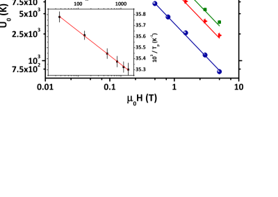
Figure 5: (Color online) Main panel: $H$-dependence of the depinning energy barriers $\langle U_{0}(H)\rangle_{pwd}$ in the three investigated samples. Data relative to SmFeAsO_0.8F_0.2 have already been reported in a previous work.Pra11 Continuous lines are best-fits to data according to a simple $1/H$ dependence. Inset: logarithmic $\nu_{m}$-dependence of $1/T_{p}$ in CeFeAsO_0.92F_0.08 ($H_{ac}=1.5$ Oe while $\mu_{0}H=1.5$ T). The continuous line is a best-fit function according to Eq. (8).

The results of the fitting procedure to $T_{p}\left(\nu_{m}\right)$ data according to Eq. (8) have been reported in the main panel of Fig. 5 for all the samples. A strongly-marked $H$-dependence of $\langle U_{0}(H)\rangle_{pwd}$ can clearly be discerned. Remarkably, a common trend is displayed for all the samples, making it possible to guess a common underlying mechanism. Beyond an overall sizeable reduction of $\langle U_{0}(H)\rangle_{pwd}$ with increasing $H$, a sharp crossover (at field values $2500$ Oe $\lesssim H_{cr}\lesssim 5000$ Oe common to all the samples) between two qualitatively different $\langle U_{0}(H)\rangle_{pwd}$ vs. $H$ regimes is observed for each sample. At low fields $H<H_{cr}$ the depinning energy $\langle U_{0}(H)\rangle_{pwd}$ is found to be only slightly dependent on $H$, while for values $H>H_{cr}$ a trend $\langle U_{0}(H)\rangle_{pwd}\propto 1/H$ can be discerned. The $1/H$ regime for depinning energies $\langle U_{0}(H)\rangle_{pwd}$ was indeed observed in different superconducting materials by means of several techniques ranging from magnetoresistivityPal90 to ac magnetometry itselfEmm91 and nuclear magnetic resonance.Rig98 This feature has already been reported in the SmFeAsO_0.8F_0.2 samplePra11 and, as it will be discussed later on, it can be justified in terms of pinning effects on a single FL propagating among bundles of entangled FLs. In this framework, the crossover between the two different trends of $\langle U_{0}(H)\rangle_{pwd}$ vs. $H$ shown in Fig. 5 can be interpreted as the transition from a basically single-flux line response at low $H$ values to a collective response of vortices for $H>5000$ Oe. The saturated low-$H$ values for the depinning energy barriers are typically $\langle U_{0}(H)\rangle_{pwd}\sim 10^{4}$ K. Such high values are in agreement with what reported from magnetoresistivity measurements in SmFeAsO_0.85 (see Ref. Lee10, ) and in Ba_1-xK_xFe₂As₂ single-crystals, even if in the latter case a much weaker $H$-dependence was observed.Wan10 These results are clearly indicative of strong intrinsic pinning of the vortex lines. Features of strong-pinning mechanisms have also been deduced in single-crystals of PrFeAsO_1-x and NdFeAsO_1-xF_x, confirming that the observed behaviour is intrinsic in REFeAsO_1-xF_x materials.VdB10

It must be noticed that, since the variation of $1/T_{p}$ vs. $\nu_{m}$ is very modest (see the vertical scale in the inset of Fig. 5), $\langle U_{0}(H)\rangle_{pwd}$ is not only determined at a fixed $H$ but almost in isothermal conditions as well. By referring to the inset of Fig. 5, in fact, one can recognize that $T_{p}(\nu_{m})$ is varying on a range of some tenths of K degree, as already observed in the case of the Sm-based sample.Pra11 This is a great advantage of the ac susceptibility technique if compared, for instance, to magnetoresistivity measurements where $\langle U_{0}(H)\rangle_{pwd}$ is estimated from an activated-like fit to data over a range of several tens of K degrees.Pal90 ; Lee10 One can then notice that the average temperature $T^{*}$ characterizing the variation of $T_{p}$ over the considered $\nu_{m}$ range is intrinsically positioned over the irreversibility line, so that the energy barrier should more correctly be referred to as $\langle U_{0}(H^{*},T^{*})\rangle_{pwd}$, where $(H^{*},T^{*})$ are the points on the $H$ – $T$ phase diagram belonging to the irreversibility line.

IV Analysis of the results

The observed behaviour can be explained by means of the phenomenological GL theoryTin96 and by referring to the model of single-vortex pinning by atomic impurities (like, for instance, ionic substitutions like O^2-/F^- or O^2- vacancies).Mal88 ; Tin88 ; Yes88 Due to the very small values of the coherence lengths $\sim 10$ Å, in fact, local defects on the atomic scale can be considered as strongly efficient pinning centers for FLs.Lee10 In this framework the energy $U_{0}$ is related to the FLs features only and does not depend on the precise pinning mechanisms.Tin88 Moreover, at strong $H$-values the high density of FLs gives rise to entangled bundles of vortices around the central one physically bound to the atomic defect.Mal88 ; Tin88 ; Yes88 Accordingly, the characteristic energy $U_{0}$ can be directly linked to the geometrical properties of the flux line lattice and, in particular, to the typical volume $V$ of the correlated vortex lines. The following phenomenological expression can be envisaged (where $U_{0}$ is expressed in K)Mal88 ; Tin88 ; Yes88

$$U_{0}(T)=\left\{\frac{H_{c}^{2}(T)}{8\pi}\right\}\frac{V}{k_{B}}$$ (9)

where the term between curly brackets quantifies the $T$-dependence of the superconducting condensation energy density. Two limiting cases can be considered.

On the one hand, by gradually increasing $H$ the density of vortices steadily increases and, accordingly, correlations among vortices increase too. A crossover to a regime where the depinning process leads to a collective response of an increasing number of vortices is then expected. In the simplified scenario of a square Abrikosov lattice of vortices, the quantity $d=\sqrt{\Phi_{0}/H}$ estimates the mutual distance among nearest neighbouring FLs. One can then assume that the correlations roughly extend over a cylindric volume whose radius is given by $d$. Namely one has $V\simeq\pi\xi(T)\Phi_{0}/H$, the characteristic size along the third dimension being determined by the coherence length.Yes88 After the substitution in Eq. (9), considerations on the powder-averaging making it possible to obtain a more convenient form in order to describe the experimental data. In particular, the following relation holds under a two-fluid approximation (see Appendix A.1 for details)

$$\langle U_{0}(H^{*},T^{*})\rangle_{pwd} = \frac{\Phi_{0}^{5/2}}{96\sqrt{2}\pi^{3/2}k_{B}}\frac{g(t^{*})\sqrt{\langle H_{c2}(0)\rangle_{pwd}}}{H^{*}}\times$$ (10)

$$\times \frac{1}{f_{1}(\gamma)\lambda_{ab}^{2}(0)}$$

where $g(t)$ is a function of $t$ and $f_{1}(\gamma)$ is a function of the anisotropy parameter $\gamma=\xi_{ab}/\xi_{c}=\lambda_{c}/\lambda_{ab}$.

On the other hand, at low enough magnetic fields the typical volume $V$ will be no longer sensitive to the presence of several flux lines but it will only be a function of the typical lengths of the single pinned vortex. As a consequence, one can consider a different cylindric volume with radius $\delta\xi(T)$. Here the heuristic parameter $\delta$ is introduced in order to grant a continuous crossover between the high- and the low-$H$ regimes.Yes88 Thus, again choosing the coherence length as the characteristic size also along the third dimension, the following relation follows

$$\langle U_{0}(H^{*},T^{*})\rangle_{pwd} = \frac{\Phi_{0}^{5/2}\delta^{2}}{192\sqrt{2}\pi^{5/2}k_{B}}\frac{h(t^{*})}{\sqrt{\langle H_{c2}(0)\rangle_{pwd}}}\times$$ (11)

$$\times \frac{1}{f_{2}(\gamma)\lambda_{ab}^{2}(0)}.$$

Here $h(t)$ is a function of $t$ and $f_{2}(\gamma)$ is a function of the anisotropy parameter (details relative to the derivation of Eq. (11) can be found in Appendix A.2).

The two resulting expressions show that in both the $H$-regimes $\lambda_{ab}(0)$ can be simply expressed as a function of the experimentally-accessible quantity $\langle U_{0}(H^{*},T^{*})\rangle_{pwd}$. One should consider that the continuity of $\lambda_{ab}(0)$ must clearly be assured at the crossover field.Yes88 The free parameters for the three different samples (namely, the anisotropy parameter $\gamma_{RE}$ and the parameter $\delta_{RE}$), anyway, make the fulfilment of this requirement quite arbitrary. Some other criterion from the analysis of experimental data should be formulated in order to derive some relations among the parameters, reducing as much as possible the degree of arbitrariness. This can be done by the examination of the FLs phase diagram and by taking into consideration the role of thermal fluctuations. As a final result of the procedure, as reported in detail in Appendix B, one finds that

$$\gamma_{Sm}^{3/2}\delta_{Sm}^{2}\simeq 1.6\gamma_{Ce}^{3/2}\delta_{Ce}^{2}\simeq 3\gamma_{La}^{3/2}\delta_{La}^{2}.$$ (12)

The linking up the different sets of data can now be performed under the fulfilment of the constraints reported in Eq. (12). As a starting point of the procedure, a reasonable value for one of the $\gamma_{RE}$ parameters should be taken as fixed. By referring to typical data reported in literature,Pal09 in particular, it will be assumed that $\gamma_{Sm}=5$. Next, data relative to the two different regimes (high- and low-$H$) in SmFeAsO_0.8F_0.2 are linked up by setting a proper value of $\delta_{Sm}$. The procedure is repeated also for Ce- and La-based samples, where the starting guesses for the parameters $\gamma_{RE}$ and $\delta_{RE}$ must be modified till the fulfilment of Eq. (12).

V Discussion

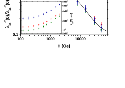
Figure 6: (Color online) Main panel: graphical representation of the collapse of experimental data represented in Fig. 5 after a proper normalization according to the value of $1/\lambda_{ab}^{2}(0)$ estimated at $250$ Oe. The continuous line is a best-fit to data according to Eq. (13). Inset: $H$-dependence of the $\lambda_{ab}(0)$ values for the three investigated samples. Open (full) symbols are relative to data from the low-$H$ (high-$H$) regime.

As reported in the inset of Fig. 6, the linking procedure of data in the two opposite limits described by Eqs. (10) and (11) under the constraints reported in Eq. (12) allows one to deduce a sizeable $H$-dependence of $\lambda_{ab}(0)$ itself. The saturation values in the limit $H\rightarrow 0$ Oe have been reported in the last column of Tab. 2 compared to the results of $\mu^{+}$SR measurements on the same samples (raw data not shown), together with the results for $\gamma_{RE}$ and $\delta_{RE}$. The presented results of $\mu^{+}$SR measurements are in good agreement with results on different samples characterized by slightly different stoichiometries.Kha08 ; Lue08 At the same time, the estimates of $\lambda_{ab}(0)$ for CeFeAsO_0.92F_0.08 and SmFeAsO_0.8F_0.2 by means of $\chi_{ac}$ are consistent with the values from $\mu^{+}$SR measurements within a systematic factor $\sim 2$. This discrepancy could possibly be accounted for by assuming that the correlations among vortices in the high-$H$ regime are actually extended over a bigger volume. In particular, it is immediate to realize that the choice of $2d$ for the cylindric volume, also implying a rescaling $\delta\rightarrow 2\delta$, leads to a complete agreement of $\chi_{ac}$ data with $\mu^{+}$SR ones.

Table 2: Parameters $\delta$, $\gamma$ and $\lambda_{ab}(0)$ (estrapolated for $H\rightarrow 0$ Oe) for the three samples resulting from the constrained linking procedure of data relative to the two distinct $H$-regimes (see text for details). Values of $\lambda_{ab}(0)$ as obtained from $\mu^{+}$SR measurements have been reported in the last column (raw data not shown in the text).

Sample	$\;\;\;\gamma\;\;\;$	$\;\;\;\delta\;\;\;$	$\lambda_{ab}(0)$ (nm)	$\lambda_{ab}(0)$ (nm)
			from $\chi_{ac}$	from $\mu^{+}$SR
LaFeAsO0.9F0.1	3.2	9.5	235 $\pm$ 15	$\diagup$
CeFeAsO0.92F0.08	4.25	10.5	128 $\pm$ 6	260 $\pm$ 15
SmFeAsO0.8F0.2	5	11.75	98 $\pm$ 8	200 $\pm$ 15

The observed behaviour of $\delta$ as a function of the RE ion can be qualitatively understood in terms of a compensation of the opposite trend in $\langle\xi\rangle_{pwd}$. The trend in the modification of the value of $\gamma$, on the other hand, can be correlated with the increase in the size of the liquid region in the phase diagram reported in Fig. 4. One can deduce that the increase in $\gamma$ possibly leads to the enhancement of 2-dimensional fluctuations, much more effective than the higher-dimensional ones in extending the liquid region of the phase diagram. It should be remarked that a similar trend in La- and Sm-based samples was reported in literature, even if the measured absolute values were considerably higher.Jar08

More interestingly, a scaling of $\lambda_{ab}^{-2}(0)$ is displayed in the main panel of Fig. 6 showing a clearly common $H$-dependence after a proper normalization with respect to the value $\lambda_{ab}^{-2}(0)$ taken at $H=250$ Oe. This feature possibly demonstrates the existence of a common material-independent underlying behaviour. It should also be remarked that the quantity $\lambda_{ab}^{-2}(0)$ is directly associated with the superfluid density $n_{s}$ of the superconducting state.Tin96 ; DeG99 This, in turn, implies that $n_{s}$ is partially suppressed by $H$ values much lower than $H_{c2}(0)$, a characteristic fingerprint of multi-gap superconductivity.Wey10 ; Kha08b By assuming a $H$-dependence typical of $s$-like bandsSon00 one can derive the following phenomenological fitting function

$$n_{s}(H)=n_{s1}+n_{s2}(H)=n_{s1}+\frac{1-n_{s1}}{1+\left(\frac{H}{H_{0}}\right)^{2}}.$$ (13)

The fitting results show that the main contribution to the superfluid density $\left(1-n_{s1}\right)\simeq 0.9$ comes from the weakest band that is suppressed by a typical magnetic field $H_{0}\simeq 1.25\times 10^{4}$ Oe. This quite unphysical result should possibly be associated with the high degree of approximation associated with the two-fluid model and the relative $T$-dependence of the characteristic lengths (see Eqs. (17) later in Appendix A.1). Our results are anyway in good qualitative agreement with previous reports obtained by means of torque magnetometry and local muon spin spectroscopy on an optimally-doped Sm-based superconductor.Wey10 In that case from $\mu^{+}$SR it was possible to deduce a weaker $H$-dependence, eventually saturating at $\mu_{0}H\sim 1.5$ T and involving the suppression of just $25$% of the overall superfluid density.

VI Conclusions

The phase diagram of the flux lines in three powder samples of REFeAsO_1-xF_x superconductors (RE = La, Ce, Sm) under conditions of nearly-optimal doping was investigated by means of ac susceptibility measurements. The irreversibility line has been estimated for the three samples, showing that in the accessible range of magnetic field the extension of the reversible liquid region is lowered with increasing $T_{c}$. This aspect could be of extreme interest in view of possible technological applications of these materials. The $H$-dependence of the characteristic depinning energy barriers was investigated in a thermally-activated framework. Results were interpreted by distinguishing two regimes of magnetic field characterized by single and collective depinning processes, allowing us to make experimental data collapse on the same temperature trend indicative of a common underlying mechanism independent on the precise material. Reliable estimates of the zero-temperature penetration depth $\lambda_{ab}(0)$ and of the RE-dependence of the anisotropy parameter $\gamma$ are finally given. Some interpretations of the observed behaviour in terms of a two-band $s^{\pm}$ model are proposed even if a refinement of the employed two-fluid model is in order.

Appendix A Derivation of the relations between $\langle U_{0}(H^{*},T^{*})\rangle_{pwd}$ and $\lambda_{ab}(0)$ in the two different $H$-regimes

A.1 Strongly correlated vortices. Depinning of bundles of flux lines

Let’s consider Eq. (9) in the limit of high-$H$, here rewritten for convenience

$$U_{0}(H,T)=\frac{H_{c}^{2}(T)}{8k_{B}}\frac{\xi(T)\Phi_{0}}{H},$$ (14)

as the starting point. By means of the GL relation for the flux quantum $\Phi_{0}=2\sqrt{2}\pi H_{c}(T)\lambda(T)\xi(T)$, one can write down an explicit expression for $U_{0}$ in different conditions of orientation of the magnetic field as follows

$$U_{0,H\parallel ab}(H,T) = \frac{\Phi_{0}^{3}}{64\pi^{2}k_{B}H}\frac{1}{\sqrt{\xi_{ab}(T)\xi_{c}(T)}\lambda_{ab}(T)\lambda_{c}(T)}$$

$$U_{0,H\parallel c}(H,T) = \frac{\Phi_{0}^{3}}{64\pi^{2}k_{B}H}\frac{1}{\xi_{ab}(T)\lambda_{ab}^{2}(T)}.$$ (15)

The expressions $\xi_{ab}/\xi_{c}=\lambda_{c}/\lambda_{ab}=\gamma$ hold for the different typical lengths in anisotropic superconductors, where $\gamma$ has already been defined in the text as the anisotropy parameter. By referring to Eq. (1) it is possible to perform a powder-like average of $U_{0}$ as

$$\langle U_{0}(H,T)\rangle_{pwd} \equiv \frac{2}{3}U_{0,H\parallel ab}(T)+\frac{1}{3}U_{0,H\parallel c}(T)={}$$

$$= \left(\frac{\sqrt{\gamma}+2}{3\gamma^{3/2}}\right)\frac{\Phi_{0}^{3}}{64\pi^{2}k_{B}H}\frac{1}{\xi_{c}(T)\lambda_{ab}^{2}(T)}.$$

In a simple two-fluid model, the $T$-dependence of $\xi_{c}(T)$ and $\lambda_{ab}(T)$ can be taken as

$$\xi_{c}(T)=\xi_{c}(0)\frac{\sqrt{1-t^{4}}}{1-t^{2}},\;\;\;\lambda_{ab}(T)=\lambda_{ab}(0)\frac{1}{\sqrt{1-t^{4}}}$$ (17)

where $t$ has already been defined as the reduced temperature $t\equiv T/T_{c}(0)$. It should be considered that, as already recalled, the estimate of $\langle U_{0}(H,T)\rangle_{pwd}$ is performed by definition at the values $(H^{*},T^{*})$ delimiting the irreversibility line. After the definition of the function $g(t)\equiv\left(1-t^{2}\right)\sqrt{1-t^{4}}$ it is then possible to write

$$\frac{\langle U_{0}(H^{*},T^{*})\rangle_{pwd}}{g(t^{*})} = \left(\frac{\sqrt{\gamma}+2}{3\gamma^{3/2}}\right)\frac{\Phi_{0}^{3}}{64\pi^{2}k_{B}H^{*}}\times$$ (18)

$$\times \frac{1}{\xi_{c}(0)\lambda_{ab}^{2}(0)}.$$

The quantity $\xi_{c}(0)$ can be independently derived by measuring the magnetic field dependence of the superconducting transition temperature $T_{c}$ by means of the relations reported in Eqs. (5) and (6) after proper considerations about the powder-average procedures. The two limiting configurations $H\parallel ab$ and $H\parallel c$ lead to the formulas

$$H_{c2,H\parallel ab}(T) = \frac{\Phi_{0}}{2\pi\xi_{ab}(T)\xi_{c}(T)},$$

$$H_{c2,H\parallel c}(T) = \frac{\Phi_{0}}{2\pi\xi_{ab}^{2}(T)}.$$ (19)

Following Eq. (1) it is possible to deduce that the experimentally-accessible quantity $\langle\xi(0)\rangle_{pwd}$, already defined in Eq. (6), is linked to $\xi_{c}(0)$ by the relation

$$\langle\xi(0)\rangle_{pwd}=\xi_{c}(0)\left(\frac{\sqrt{3}\gamma}{\sqrt{2\gamma+1}}\right).$$ (20)

Coming back to Eq. (18), one can substitute Eqs. (20) and (6) to obtain

$$\frac{\langle U_{0}(H^{*},T^{*})\rangle_{pwd}}{g(t^{*})\sqrt{\langle H_{c2}(0)\rangle_{pwd}}} = \frac{\Phi_{0}^{5/2}}{96\sqrt{2}\pi^{3/2}k_{B}}\times$$ (21)

$$\times \frac{1}{f_{1}(\gamma)\lambda_{ab}^{2}(0)}\frac{1}{H^{*}}$$

having defined the function of the anisotropy parameter

$$f_{1}(\gamma)=\frac{1}{\sqrt{3}}\frac{\sqrt{2\gamma^{2}+\gamma}}{\sqrt{\gamma}+2}.$$ (22)

Eq. (21) is equivalent to Eq. (10).

A.2 Weakly correlated vortices. Depinning of single flux lines

Let’s now consider Eq. (9) in the limit of low-$H$, here rewritten for convenience

$$U_{0}(T)=\frac{H_{c}^{2}(T)}{8k_{B}}\delta^{2}\xi^{3}(T).$$ (23)

Again by means of the GL relation for the flux quantum $\Phi_{0}=2\sqrt{2}\pi H_{c}(T)\lambda(T)\xi(T)$ it is possible to explicit the expressions for $U_{0}$ in the different cases of the orientation of the system with respect to the magnetic field as

$$U_{0,H\parallel ab}(T) = \frac{\Phi_{0}^{2}\delta^{2}}{64\pi^{2}k_{B}}\frac{\sqrt{\xi_{ab}(T)\xi_{c}(T)}}{\lambda_{ab}(T)\lambda_{c}(T)}$$

$$U_{0,H\parallel c}(T) = \frac{\Phi_{0}^{2}\delta^{2}}{64\pi^{2}k_{B}}\frac{\xi_{ab}(T)}{\lambda_{ab}^{2}(T)}.$$ (24)

Similarly to what performed in the previous Appendix concerning strongly correlated vortices, the $\gamma$ factor can be introduced and $\lambda_{ab}(T)$, $\xi_{c}(T)$ can be left as independent quantities. By considering that the estimate of $\langle U_{0}(H,T)\rangle_{pwd}$ is performed along the irreversibility line $(H^{*},T^{*})$, by employing Eq. (17) and after a powder-like average of the energy barrier one can write

$$\frac{\langle U_{0}(H^{*},T^{*})\rangle_{pwd}}{h(t^{*})} = \left(\frac{\gamma^{2}+2\sqrt{\gamma}}{3\gamma}\right)\frac{\Phi_{0}^{2}\delta^{2}}{64\pi^{2}k_{B}}\times$$ (25)

$$\times \frac{\xi_{c}(0)}{\lambda_{ab}^{2}(0)}$$

where $h(t)\equiv\left(1+t^{2}\right)\sqrt{1-t^{4}}$. By again expressing $\xi_{c}(0)$ in terms of $\langle H_{c2}(0)\rangle_{pwd}$ through Eq. (20) and by means of Eq. (6), it is finally possible to deduce the following expression

$$\frac{\langle U_{0}(H^{*},T^{*})\rangle_{pwd}\sqrt{\langle H_{c2}(0)\rangle_{pwd}}}{h(t^{*})} = \frac{\Phi_{0}^{5/2}\delta^{2}}{192\sqrt{2}\pi^{5/2}k_{B}}\times$$ (26)

$$\times \frac{1}{f_{2}(\gamma)\lambda_{ab}^{2}(0)}.$$

In the previous expression, $f_{2}(\gamma)$ is defined as

$$f_{2}(\gamma)=\frac{\sqrt{3}\gamma^{2}}{\left(\gamma^{2}+2\sqrt{\gamma}\right)\sqrt{2\gamma+1}}.$$ (27)

Eq. (26) is equivalent to Eq. (11).

Appendix B Linking procedure of data in the two different $H$-regimes

In this Appendix the problem of the continuity at the crossover field $H_{cr}$ of the $\lambda_{ab}(0)$ vs. $H$ data, obtained by means of Eqs. (10) and (11), will be considered. In particular, as already stated in the text, some constraints on the variability of the six parameters $\gamma_{RE}$ and $\delta_{RE}$ (RE = La, Ce, Sm) should be fixed in order to reduce as much as possible the degree of arbitrariness of the procedure of data-linking.

At this aim, it is convenient to introduce the Ginzburg-Levanyuk number $\widetilde{Gi}_{3D}(0)$ asLar05

$$\widetilde{Gi}_{3D}(0)=\frac{1}{2}\left[\frac{8\pi^{2}k_{B}T_{c}(0)\lambda^{2}(0)}{\Phi_{0}^{2}\xi(0)}\right]^{2}$$ (28)

quantifying the extension of the region of the $H-T$ phase diagram where thermal fluctuations are sizeable and significantly affect the physics of the system. The $H$-dependence of $\widetilde{Gi}_{3D}(0)$ is given byLar05

$$Gi_{3D}(0,H)=\left[\frac{2H\sqrt{\widetilde{Gi}_{3D}(0)}}{H_{c2}(0)}\right]^{2/3}.$$ (29)

In fact, one can assume that the position of the irreversibility line is mainly governed by the amount of thermal fluctuations in the system. As a consequence, $Gi_{3D}(0,H)$ is expected to be directly involved in the analytic expression relative to the irreversibility line itself. One hint at the correctness of this picture is possibly given by the similarity between the characteristic exponents observed in Eqs. (7) and (29). Similar considerations, moreover, have already been proposed in literature concerning the thermodynamical melting line (see, in particular, Sections IV and V of Ref. Bla94, and references therein. In that case, anyway, the considered exponent is $\beta=2$). The following expression for the irreversibility line can then be considered

$$1-\frac{T^{*}}{T_{c}(0)}=\frac{Gi_{3D}(0,H^{*})}{K^{2/3}}$$ (30)

where $K$ is an arbitrary proportionality factor. Together with Eq. (29), this straightforwardly leads to

$$\frac{2H^{*}\sqrt{\widetilde{Gi}_{3D}(0)}}{H_{c2}(0)}=K\left[1-\frac{T^{*}}{T_{c}(0)}\right]^{3/2}$$ (31)

Since all the sample-dependent quantities are already kept into consideration by $\widetilde{Gi}_{3D}(0)$, it is reasonable to assume $K$ as a sample-independent parameter. $K$ can typically be interpreted in terms of microscopic properties of the vortices.Bla94 In the present phenomenological model, anyway, such microscopic interpretations are left aside.

In order to give a suitable description of the experimental data, Eq. (31) should be powder-averaged by considering the criterion already presented in Eq. (1). By considering the definition of $\widetilde{Gi}_{3D}(0)$ reported in Eq. (28), one can write

$$\frac{\sqrt{\widetilde{Gi}_{3D}(0)}}{H_{c2}(0)} = \frac{1}{\sqrt{2}}\frac{8\pi^{2}k_{B}T_{c}(0)\lambda_{ab}(0)\lambda_{c}(0)}{\Phi_{0}^{2}\sqrt{\xi_{ab}(0)\xi_{c}(0)}}\frac{2\pi\xi_{ab}(0)\xi_{c}(0)}{\Phi_{0}}$$

$$\frac{\sqrt{\widetilde{Gi}_{3D}(0)}}{H_{c2}(0)} = \frac{1}{\sqrt{2}}\frac{8\pi^{2}k_{B}T_{c}(0)\lambda_{ab}^{2}(0)}{\Phi_{0}^{2}\xi_{ab}(0)}\frac{2\pi\xi_{ab}^{2}(0)}{\Phi_{0}}$$ (32)

for the two field orientations $H\parallel ab$ and $H\parallel c$, respectively. By again performing the powder-average procedure and after introducing the anisotropy parameter through the relations $\xi_{ab}/\xi_{c}=\lambda_{c}/\lambda_{ab}=\gamma$, by referring to Eqs. (6) and (20) one obtains the following expression

$$\left\langle\frac{\sqrt{\widetilde{Gi}_{3D}(0)}}{H_{c2}(0)}\right\rangle_{pwd} = \frac{1}{f_{3}(\gamma)}\frac{8\pi^{2}k_{B}T_{c}(0)\lambda_{ab}^{2}(0)}{\sqrt{2}\Phi_{0}^{2}\xi_{c}(0)}\times$$ (33)

$$\times \frac{1}{\langle H_{c2}(0)\rangle_{pwd}}$$

where the function $f_{3}(\gamma)$ is defined as

$$f_{3}(\gamma)=\frac{9\gamma^{2}}{\left(2\gamma^{3/2}+\gamma\right)\left(2\gamma+1\right)}.$$ (34)

One should now consider that the definition of $\widetilde{Gi}_{3D}(0)$ reported in Eq. (28) does not account for any $H$-dependence that is fully accounted for by Eq. (29). Eq. (33) is then referred to a $H=0$ Oe condition and, as a consequence, the quantity $\lambda_{ab}^{2}(0)/\xi_{c}(0)$ can be obtained by means of Eq. (25) (holding in the low-$H$ regime). By inserting the resulting expression into Eq. (31) one obtains

$$\frac{H^{*}}{\langle H_{c2}(0)\rangle_{pwd}}\simeq\widetilde{K}_{RE}\times\left[0.95-\frac{T^{*}}{T_{c}(0)}\right]^{3/2}$$ (35)

where

$$\widetilde{K}_{RE}\equiv\left\{\frac{\langle U_{0}(H^{*},T^{*})\rangle_{pwd}}{T_{c}(0)h(t^{*})}\right\}_{RE}\times\frac{27\sqrt{2}}{\gamma_{RE}^{3/2}\delta_{RE}^{2}}K.$$ (36)

As already discussed in the text, the factor $0.95$ in Eq. (35) phenomenologically accounts for the definition of the irreversibility line from the $\chi_{ac}^{\prime\prime}$-criterion.

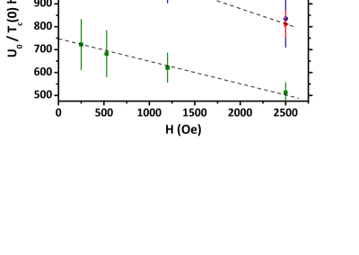
Figure 7: (Color online) Graphical representation of the quantity between square brackets in Eq. (36). The dashed lines are guides for the eye and they can be used to extrapolate the intercept values back to $H=0$ Oe.

The quantity between curly brackets in Eq. (36) can be experimentally estimated from a linear extrapolation of the intercept values back to $H=0$ Oe (see Fig. 7). One can then compare the sample-dependent quantity $\widetilde{K}_{RE}$ with the corresponding experimental quantities derived from the fitting procedure shown in Fig. 4. Together with the already cited assumption that $K$ is a sample-independent quantity, this implies that some constraints can be put on the variability of the parameters $\gamma_{RE}$ and $\delta_{RE}$. In particular, one finds that

$$\gamma_{Sm}^{3/2}\delta_{Sm}^{2}\simeq 1.6\gamma_{Ce}^{3/2}\delta_{Ce}^{2}\simeq 3\gamma_{La}^{3/2}\delta_{La}^{2},$$ (37)

as reported in Eq. (12).

References

- (1) Y. Kamihara, T. Watanabe, M. Hirano, H. Hosono, J. Am. Chem. Soc. 130, 3296 (2008)
- (2) R. H. Liu, T. Wu, G. Wu, H. Chen, X. F. Wang, Y. L. Xie, J. J. Ying, Y. J. Yan, Q. J. Li, B. C. Shi, W. S. Chu, Z. Y. Wu, X. H. Chen, Nature 459, 64 (2009)
- (3) L. Boeri, O. V. Dolgov, A. A. Golubov, Phys. Rev. Lett. 101, 026403 (2008)
- (4) R. S. Gonnelli, D. Daghero, G. A. Ummarino, V. A. Stepanov, J. Jun, S. M. Kazakov, J. Karpinski, Phys. Rev. Lett. 89, 247004 (2002)
- (5) A. Bussmann Holder, A. Simon, H. Keller, A. R. Bishop, J. Supercond. Nov. Magn. 23, 365 (2010)
- (6) G. A. Ummarino, Phys. Rev. B 83, 092508 (2011)
- (7) F. Hunte, J. Jaroszynski, A. Gurevich, D. C. Larbalestier, R. Jin, A. S. Sefat, M. A. McGuire, B. C. Sales, D. K. Christen, D. Mandrus, Nature 453, 903 (2008)
- (8) D. Daghero, M. Tortello, R. S. Gonnelli, V. A. Stepanov, N. D. Zhigadlo, J. Karpinski, Phys. Rev. B 80, 060502(R) (2009)
- (9) H.-S. Lee, M. Bartkowiak, J.-H. Park, J.-Y. Lee, J.-Y. Kim, N.-H. Sung, B. K. Cho, C.-U. Jung, J. S. Kim, H.-J. Lee, Phys. Rev. B 80, 144512 (2009)
- (10) S. Weyeneth, M. Bendele, R. Puzniak, F. Murányi, A. Bussmann-Holder, N. D. Zhigadlo, S. Katrych, Z. Bukowski, J. Karpinski, A. Shengelaya, R. Khasanov, H. Keller, Europhys. Lett. 91, 47005 (2010)
- (11) R. Khasanov, D. V. Evtushinsky, A. Amato, H.-H. Klauss, H. Luetkens, C. Niedermayer, B. Buchner, G. L. Sun, C. T. Lin, J. T. Park, D. S. Inosov, V. Hinkov, Phys. Rev. Lett. 102, 187005 (2009)
- (12) R. Khasanov, M. Bendele, A. Amato, K. Conder, H. Keller, H.-H. Klauss, H. Luetkens, E. Pomjakushina, Phys. Rev. Lett. 104, 087004 (2010)
- (13) G. Prando, P. Carretta, R. De Renzi, S. Sanna, A. Palenzona, M. Putti, M. Tropeano, Phys. Rev. B 83, 174514 (2011)
- (14) D. C. Johnston, Adv. Phys. 59, 803 (2010)
- (15) G. Prando, A. Lascialfari, A. Rigamonti, L. Romano, S. Sanna, M. Putti, M. Tropeano, Phys. Rev. B 84, 064507 (2011)
- (16) A. Kondrat, J. E. Hamann-Borrero, N. Leps, M. Kosmala, O. Schumann, A. Köhler, J. Werner, G. Behr, M. Braden, R. Klingeler, B. Büchner, C. Hess, Eur. Phys. J. B 70, 461 (2009)
- (17) X. Zhu, H. Yang, L. Fang, G. Mu, H.-H. Wen, Supercond. Sci. Technol. 21, 105001 (2008)
- (18) M. Nikolo, R. B. Goldfarb, Phys. Rev. B 39, 6615 (1989)
- (19) F. Gömöry, Supercond. Sci. Technol. 10, 523 (1997)
- (20) A. P. Malozemoff, T. K. Worthington, Y. Yeshurun, F. Holtzberg, P. H. Kes, Phys. Rev. B 38, 7203(R) (1988)
- (21) M. Tinkham, Phys. Rev. Lett. 61, 1658 (1988)
- (22) C. J. van der Beek, P. H. Kes, Phys. Rev. B 43, 13032 (1991)
- (23) C. J. van der Beek, V. B. Geshkenbein, V. M. Vinokur, Phys. Rev. B 48, 3393 (1993)
- (24) D. N. Zheng, A. M. Campbell, J. D. Johnson, J. R. Cooper, F. J. Blunt, A. Porch, P. A. Freeman, Phys. Rev. B 49, 1417 (1994)
- (25) E. H. Brandt, Phys. Rev. Lett. 67, 2219 (1991)
- (26) M. W. Coffey, J. R. Clem, Phys. Rev. B 45, 9872 (1992)
- (27) R. Prozorov, R. W. Giannetta, N. Kameda, T. Tamegai, J. A. Schlueter, P. Fournier, Phys. Rev. B 67, 184501 (2003)
- (28) P. Prommapan, M. A. Tanatar, B. Lee, S. Khim, K. H. Kim, R. Prozorov, Phys. Rev. B 84, 060509(R) (2011)
- (29) Y. Yeshurun, A. P. Malozemoff, A. Shaulov, Rev. Mod. Phys. 68, 911 (1996)
- (30) T. T. M. Palstra, B. Batlogg, R. B. van Dover, L. F. Schneemeyer, J. V. Waszczak, Phys. Rev. B 41, 6621 (1990)
- (31) J. H. P. M. Emmen, V. A. M. Brabers, W. J. M. de Jonge, Physica C 176, 137 (1991)
- (32) M. Tinkham, Physica B 169, 66 (1991)
- (33) A. Gurevich, Phys. Rev. B 67, 184515 (2003)
- (34) N. R. Werthamer, E. Helfand, P. C. Hohenberg, Phys. Rev. 147, 295 (1966)
- (35) M. Tinkham, Introduction to Superconductivity, McGraw-Hill Book Co. (1996)
- (36) P. G. de Gennes, Superconductivity of Metals and Alloys, Westview Press (1999)
- (37) Y. Yeshurun, A. P. Malozemoff, Phys. Rev. Lett. 60, 2202 (1988)
- (38) R. Prozorov, N. Ni, M. A. Tanatar, V. G. Kogan, R. T. Gordon, C. Martin, E. C. Blomberg, P. Prommapan, J. Q. Yan, S. L. Bud’ko, P. C. Canfield, Phys. Rev. B 78, 224506 (2008)
- (39) A. Rigamonti, F. Borsa, P. Carretta, Rep. Prog. Phys. 61, 1367 (1998)
- (40) H.-S. Lee, M. Bartkowiak, J. S. Kim, H.-J. Lee, Phys. Rev. B 82, 104523 (2010)
- (41) X.-L. Wang, S. R. Ghorbani, S.-I. Lee, S. X. Dou, C. T. Lin, T. H. Johansen, K.-H. Muller, Z. X. Cheng, G. Peleckis, M. Shabazi, A. J. Qviller, V. V. Yurchenko, G. L. Sun, D. L. Sun, Phys. Rev. B 82, 024525 (2010)
- (42) C. J. van der Beek, G. Rizza, M. Konczykowski, P. Fertey, I. Monnet, T. Klein, R. Okazaki, M. Ishikado, H. Kito, A. Iyo, H. Eisaki, S. Shamoto, M. E. Tillman, S. L. Bud’ko, P. C. Canfield, T. Shibauchi, Y. Matsuda, Phys. Rev. B 81, 174517 (2010)
- (43) I. Pallecchi, C. Fanciulli, M. Tropeano, A. Palenzona, M. Ferretti, A. Malagoli, A. Martinelli, I. Sheikin, M. Putti, C. Ferdeghini, Phys. Rev. B 79, 104515 (2009)
- (44) R. Khasanov, H. Luetkens, A. Amato, H.-H. Klauss, Z.-A. Ren, J. Yang, W. Lu, Z.-X. Zhao, Phys. Rev., B 78, 092506 (2008)
- (45) H. Luetkens, H.-H. Klauss, R. Khasanov, A. Amato, R. Klingeler, I. Hellmann, N. Leps, A. Kondrat, C. Hess, A. Kohler, G. Behr, J. Werner, B. Buchner, Phys. Rev. Lett. 101, 097009 (2008) and references therein
- (46) J. Jaroszynski, S. C. Riggs, F. Hunte, A. Gurevich, D. C. Larbalestier, G. S. Boebinger, F. F. Balakirev, A. Migliori, Z. A. Ren, W. Lu, J. Yang, X. L. Shen, X. L. Dong, Z. X. Zhao, R. Jin, A. S. Sefat, M. A. McGuire, B. C. Sales, D. K. Christen, D. Mandrus, Phys. Rev. B 78, 064511 (2008)
- (47) R. Khasanov, P. W. Klamut, A. Shengelaya, Z. Bukowski, I. M. Savic, C. Baines, H. Keller, Phys. Rev. B 78, 014502 (2008)
- (48) J. E. Sonier, J. H. Brewer, R. F. Kiefl, Rev. Mod. Phys. 72, 769 (2000)
- (49) A. Larkin, A. Varlamov, Theory of Fluctuations in Superconductors, Oxford Science Publications (2005)
- (50) G. Blatter, M. V. Feigel’man, V. B. Geshkenbein, A. I. Larkin, V. M. Vinokur, Rev. Mod. Phys. 66, 1125 (1994)