The Maximum Clique Problem in Multiple Interval Graphs

Abstract

Multiple interval graphs are variants of interval graphs where instead of a single interval, each vertex is assigned a set of intervals on the real line. We study the complexity of the MAXIMUM CLIQUE problem in several classes of multiple interval graphs. The MAXIMUM CLIQUE problem, or the problem of finding the size of the maximum clique, is known to be NP-complete for $t$-interval graphs when $t\geq 3$ and polynomial-time solvable when $t=1$. The problem is also known to be NP-complete in $t$-track graphs when $t\geq 4$ and polynomial-time solvable when $t\leq 2$. We show that MAXIMUM CLIQUE is already NP-complete for unit 2-interval graphs and unit 3-track graphs. Further, we show that the problem is APX-complete for 2-interval graphs, 3-track graphs, unit 3-interval graphs and unit 4-track graphs. We also introduce two new classes of graphs called $t$-circular interval graphs and $t$-circular track graphs and study the complexity of the MAXIMUM CLIQUE problem in them. On the positive side, we present a polynomial time $t$-approximation algorithm for WEIGHTED MAXIMUM CLIQUE on $t$-interval graphs, improving earlier work with approximation ratio $4t$.

1 Introduction

Given a family of sets $\mathcal{F}$, a graph $G$ with vertex set $V(G)$ and edge set $E(G)$ is said to be an “intersection graph of sets from $\mathcal{F}$” if $\exists f:V(G)\rightarrow\mathcal{F}$ such that for distinct $u,v\in V(G)$, $uv\in E(G)\Leftrightarrow f(u)\cap f(v)\not=\emptyset$. When $\mathcal{F}$ is the set of all closed intervals on the real line, it defines the well-known class of interval graphs. A $t$-interval is the union of $t$ intervals on the real line. When $\mathcal{F}$ is the set of all $t$-intervals, it defines the class of graphs called $t$-interval graphs. This class was first defined and studied by Trotter and Harary [24]. Given $t$ parallel lines (or tracks), if each element of $\mathcal{F}$ is the union of $t$ intervals on different lines, one defines the class of $t$-track graphs. It is easy to see that this class forms a subclass of $t$-interval graphs.

These classes of graphs received a lot of attention, for both their theoretical simplicity and their use in various fields like Scheduling [3, 12] or Computational Biology [2, 8]. West and Shmoys [26] showed that recognizing $t$-interval graphs for $t\geq 2$ is NP-complete.

Given a circle, the intersection graphs of arcs of this circle forms the class of circular arc graphs. We introduce similar generalizations of circular arc graphs. If $G$ has an intersection representation using $t$ arcs on a circle per vertex, then $G$ is called a $t$-circular interval graph. If instead, $G$ has an intersection representation using $t$ circles and exactly one arc on each circle corresponding to each vertex of $G$, then $G$ is called a $t$-circular track graph. Note that in this case, the class of $t$-circular track graphs may not be a subclass of the class of $t$-circular interval graphs. One can see after cutting the circles, that $t$-circular interval graphs and $t$-circular track graphs are respectively contained in $(t+1)$- and $(2t)$-interval graphs.

For all these intersection families of graphs, one can define a subclass where all the intervals or arcs have the same length. We respectively call those subclasses unit $t$-interval, unit $t$-track, unit $t$-circular interval, and unit $t$-circular track graphs.

MAXIMUM WEIGHTED CLIQUE is the problem of deciding, given a graph $G$ with weighted vertices and an integer $k$, whether $G$ has a clique of weight $k$. The case where all the weights are 1 is MAXIMUM CLIQUE. Zuckerman [27] showed that unless P=NP, there is no polynomial time algorithm that approximates the maximum clique within a factor $O(n^{1-\epsilon})$, for any $\epsilon>0$. MAXIMUM CLIQUE has been studied for many intersection graphs families. It has been shown to be polynomial for interval filament graphs [11], a graph class including circle graphs, chordal graphs and co-comparability graphs. It has been shown to be NP-complete for $B_{1}$-VPG graphs [19] (intersection of strings with one bend and axis-parallel parts [1]), and for segment graphs [6] (answering a conjecture of Kratochvíl and Nešetřil [18]).

MAXIMUM CLIQUE is polynomial for interval graphs (folklore) and for circular interval graphs [10, 13]. However, Butman et al. [5] showed that MAXIMUM CLIQUE is NP-complete for $t$-interval graphs when $t\geq 3$. For $t$-track graphs, MAXIMUM CLIQUE is polynomial-time solvable when $t\leq 2$ and NP-complete when $t\geq 4$ [17]. Butman et al. also showed a polynomial-time $\frac{t^{2}-t+1}{2}$ factor approximation algorithm for MAXIMUM CLIQUE in $t$-interval graphs. Koenig [17] observed that a similar approximation algorithm with a slightly better approximation ratio $\frac{t^{2}-t}{2}$ exists for MAXIMUM CLIQUE in $t$-track graphs. Butman et al. asked the following questions:

• Is MAXIMUM CLIQUE NP-hard in 2-interval graphs?

• Is it APX-hard in $t$-interval graphs for any constant $t\geq 2$?

• Can an algorithm with a better approximation ratio than $\frac{t^{2}-t+1}{2}$ be achieved for $t$-interval graphs?

We answer all of these questions in the affirmative. As far as the third question is concerned, Kammer, Tholey and Voepel [16] have already presented an improved polynomial-time approximation algorithm that achieves an approximation ratio of $4t$ for $t$-interval graphs. In this paper (Section 3), we present a linear time $2t$-approximation algorithm, and a polynomial time $t$-approximation algorithm for MAXIMUM WEIGHTED CLIQUE in $t$-interval graphs (and thus in $t$-track graphs), $t$-circular interval graphs, and $t$-circular track graphs. Then we show in Section 4 that MAXIMUM CLIQUE is APX-complete for many of these families (including 2-interval graphs). In Section 5, we show that for some of the remaining classes (including unit 2-interval graphs) MAXIMUM CLIQUE is NP-complete. In Section 6 we give some APX-hardness results for several problems restricted to the complement class of $t$-interval graphs. Finally, we conclude with some remarks and open questions.

2 Preliminaries

Consider a circle $C$ of length $l$ with a distinguished point $O$. The coordinate of a point $p\in C$ is the length of the arc going clockwise from $O$ to $p$. Given two reals $p$ and $q$, $[p,q]$ is the arc of $C$ going clockwise from the point with coordinate $p$ to the one with coordinate $q$. In the following, coordinates are understood modulo $l$.

A representation of a $t$-interval graph $G$ is a set of $t$ functions, $I_{1},\ldots,I_{t}$, assigning each vertex in $V(G)$ to an interval of the real line. For $t$-track graphs we have $t$ lines $L_{1},\ldots,L_{t}$, and each $I_{i}$ assigns intervals from $L_{i}$. Similarly, for a representation of $t$-circular interval graphs (resp. $t$-circular track graphs) we have a circle $C$ (resp. $t$ circles $C_{1},\ldots,C_{t}$) and $t$ functions $I_{i}$, assigning each vertex in $V(G)$ to an arc of $C$ (resp. of $C_{i}$).

3 Approximation algorithms

The first approximation algorithms for the MAXIMUM CLIQUE in $t$-interval graphs and $t$-track graphs [5, 17] are based on the fact that any $t$-interval representation (resp. $t$-track representation) of a clique admits a transversal (i.e. a set of points touching at least one interval of each vertex) of size $\tau=t^{2}-t+1$ (resp. $\tau=t^{2}-t$) [15]. Scanning the representation of a graph $G$ from left to right (in time $O(tn)$) one passes through the points of the transversal of a maximum clique $K$ of $G$. At some of those points there are at least $|K|/\tau$ intervals forming a subclique of $K$. Thus, this gives an $O(tn)$-time $\tau$-approximation. Butman et al. improved this ratio by 2 by considering every pair of points in the representation. The intervals at these points induce a co-bipartite graph, for which computing the maximum clique is polynomial (as computing a maximum independent set of a bipartite graph is polynomial). Then one can see that this gives a polynomial time $(\tau/2)$-approximation algorithm. This actually gives a polynomial exact algorithm for the MAXIMUM CLIQUE in $2$-track graphs [17], as $\tau=2$ in this case. For the other cases, Kammer et al. [16] greatly improved the approximation ratios from roughly $t^{2}/2$ to $4t$, using the new notion of $k$-perfect orientability. Using transversal arguments, we can easily improve this ratio for some subclasses. A representation is balanced if for each vertex, all its intervals (or arcs) have the same length.

Remark 1

In any balanced $t$-interval (resp. $t$-track, $t$-circular interval, or $t$-circular track) representation of a clique, the $2t$ interval extremities of the vertex with the smallest intervals form a transversal. Thus, in those classes of graphs MAXIMUM CLIQUE admits a linear time $2t$-approximation algorithm, and a polynomial time $t$-approximation algorithm.

We shall now show how to achieve the same approximation ratio without restraining to balanced representations.

Theorem 3.1

There is a linear time $2t$-approximation algorithm, and a polynomial time $t$-approximation algorithm for MAXIMUM WEIGHTED CLIQUE on $t$-interval graphs, $t$-track graphs, $t$-circular interval graphs, and $t$-circular track graphs.

Proof

The problem is polynomial when $t=1$, we thus assume that $t\geq 2$. Let us prove the theorem for $t$-interval graphs, the proofs for the other classes are exactly the same. Let $G$ be a weighted $t$-interval graph with weight function $w(u)$ on its vertices, and let $K$ be a maximum weighted clique of $G$. Let $I_{1},\ldots,I_{t}$ form a $t$-interval representation of $G$ such that for any vertex $u\in V(G)$, $I_{i}(u)=[u_{i},u^{\prime}_{i}]$. For any edge $uv$ there exists a $i$ and a $j\in[t]$ such that the point $u_{i}$ belongs to $I_{j}(v)$, or such that $v_{j}\in I_{i}(u)$. One can thus orient and color the edges of $G$ in such a way that $uv$ goes from $u$ to $v$ in color $i$ if $u_{i}\in I_{j}(v)$ for some $j$. In $K$ there is a vertex $u$ with more weight on its out-neighbors in $K$ than on its in-neighbors in $K$. Indeed, this comes from the fact that in the oriented graphs obtained from $K$ by replacing each vertex $u$ by $w(u)$ vertices $u_{i}$ and by putting an arc $u_{i}v_{j}$ if and only if there is an arc $uv$ in $K$, there is a vertex $u_{i}$ with $d^{+}(u_{i})\geq d^{-}(u_{i})$, which is equivalent to $w(N^{+}_{K}(u))\geq w(N^{-}_{K}(u))$. Thus there exists two distinct values $i$ and $j$ such that $u$ has at least weight $(w(K)-w(u))/2t$ on its out-neighbors in color $i$, and at least $(w(K)-w(u))/t$ out-neighbors in color $i$ or $j$. The vertex $u$ and its out-neighbors in a given color clearly induce a clique of $G$ (they intersect at $u_{i}$). Thus scanning the representation from left to right looking for the point with the more weights gives a clique of weight at least $w(u)+(w(K)-w(u))/2t>w(K)/2t$, which is a $2t$-approximation.

Then the graph induced by $u$ and its out-neighbors in color $i$ or $j$ being co-bipartite one can compute its maximum weighted clique in polynomial time (as computing a maximum weighted independent set of a bipartite graph is polynomial). This clique has weight at least $w(u)+(w(K)-w(u))/t>w(K)/t$ (the weight of the subclique of $K$ induced by $u$ and its neighbors in color $i$ or $j$). Thus, for each vertex $u$ of the graph and any pair $u_{i}$ and $u_{j}$ of interval left end, if we compute the maximum weighted clique of the corresponding co-bipartite graph, we obtain a $t$-approximation.

4 APX-hardness in multiple interval graphs

The complement of a graph $G$ is denoted by $\overline{G}$. Given a graph $G$ on $n$ vertices with $V(G)=\{x_{1},\ldots,x_{n}\}$ and $E(G)=\{e_{1},\ldots,e_{m}\}$, and a positive integer $w$, we define $Subd_{w}(G)$ to be the graph obtained by subdividing each edge of $G$ $w$ times. If $e_{k}\in E(G)$ and $e_{k}=x_{i}x_{j}$ where $i<j$, we define $l(k)=i$ and $r(k)=j$ (as if $x_{i}$ and $x_{j}$ were respectively the left and the right end of $e_{k}$). In the following we subdivide edges 2 or 4 times. In $Subd_{2}(G)$ (resp. $Subd_{4}(G)$), the vertices subdividing $e_{k}$ are $a_{k}$ and $b_{k}$ (resp. $a_{k},b_{k},c_{k},$ and $d_{k}$) and they are such that $(x_{l(k)},a_{k},b_{k},x_{r(k)})$ (resp. $(x_{l(k)},a_{k},b_{k},c_{k},d_{k},x_{r(k)})$) is the subpath of $Subd_{2}(G)$ (resp. $Subd_{4}(G)$) corresponding to $e_{k}$. To prove APX-hardness results we need the following structural theorem, which is of independent interest.

Theorem 4.1

Given any graph $G$,

• $\overline{Subd_{4}(G)}$ is a 2-interval graph,

• $\overline{Subd_{2}(G)}$ is a unit 3-interval graph,

• $\overline{Subd_{2}(G)}$ is a 3-track graph,

• $\overline{Subd_{2}(G)}$ is a unit 4-track graph,

• $\overline{Subd_{2}(G)}$ is a unit 2-circular interval graph (and thus a 2-circular interval graph),

• $\overline{Subd_{2}(G)}$ is a 2-circular track graph, and

• $\overline{Subd_{2}(G)}$ is a unit 4-circular track graph.

Furthermore, such representations can be constructed in linear time.

Since MAXIMUM INDEPENDENT SET is APX-hard even when restricted to degree bounded graphs [21, 4], Chlebík and Chelbíková [7] observed that MAXIMUM INDEPENDENT SET is APX-hard even when restricted to $2k$-subdivisions of 3-regular graphs for any fixed integer $k\geq 0$. Taking the complement graphs, we thus have that MAXIMUM CLIQUE is APX-hard even when restricted to the set ${\mathcal{C}}_{2k}=\{\overline{Subd_{2k}(G)}\ |$ any graph $G\}$, for any fixed integer $k\geq 0$. Thus, since MAXIMUM CLIQUE is approximable for all the graph classes considered in Theorem 4.1, we clearly have the next result.

Theorem 4.2

MAXIMUM CLIQUE is APX-complete for:

• 2-interval graph,

• unit 3-interval graph,

• 3-track graph,

• unit 4-track graph,

• unit 2-circular interval graph (and thus for 2-circular interval graphs),

• 2-circular track graph, and

• unit 4-circular track graph.

Remark 2

To prove that MAXIMUM CLIQUE is NP-hard on $B_{1}$-VPG graphs, Middendorf and Pfeiffer [19] proved that for any graph $G$, $\overline{Subd_{2}(G)}\in B_{1}$-VPG. One can thus see that MAXIMUM CLIQUE is actually APX-hard for this class of graphs.

We prove Theorem 4.1 in the following subsections.

4.1 2-interval graphs

Theorem 4.3

Given any graph $G$, $\overline{Subd_{4}(G)}$ is a 2-interval graph and a 2-interval representation for it can be constructed in linear time.

Proof

Recall that each edge $e_{k}=x_{i}x_{j}$ of $G$ where $i<j$, corresponds to the path $(x_{i},a_{k},b_{k},c_{k},d_{k},x_{j})$ in $Subd_{4}(G)$. We define the representation $\{I_{1},I_{2}\}$ of $\overline{Subd_{4}(G)}$ as follows (see also Figure 1). For $1\leq i\leq n$ and $1\leq k\leq m$:

$\begin{array}[]{lcl}I_{1}(a_{k})&=&[0,m(l(k)-1)+k-1]\\ I_{1}(x_{i})&=&[mi,mn+mi]\\ I_{2}(a_{k})&=&[mn+ml(k)+1,4mn+m-ml(k)-k+1]\\ I_{1}(b_{k})&=&[m(l(k)-1)+k,mn+m-k]\\ I_{1}(c_{k})&=&[mn+m-k+1,3mn+m-mr(k)-k+1]\\ I_{1}(d_{k})&=&[3mn+m-mr(k)-k+2,4mn+mr(k)]\\ I_{2}(b_{k})&=&[4mn+m-ml(k)-k+2,5mn+k]\\ I_{2}(x_{i})&=&[4mn+mi+1,5mn+mi+1]\\ I_{2}(d_{k})&=&[5mn+mr(k)+k+1,6mn+m+1]\\ I_{2}(c_{k})&=&[5mn+k+1,5mn+mr(k)+k]\end{array}$

Figure 1: The 2-interval representation of $\overline{Subd_{4}(G)}$.

Figure 1 (and the other figures of this kind) should be understood in the following way. The leftmost block labeled $a_{k}$ corresponds to the intervals $I_{1}(a_{k})$, and its shape, together with the label $(l(k),k)$ on the arrow mean that,

• the left end of the intervals $I_{1}(a_{k})$ are the same (coordinate 0), and that

• the right end of the intervals $I_{1}(a_{k})$ are ordered (from left to right) accordingly to $l(k)$, and in case of equality, accordingly to $k$.

Here we can see that this block is close to the blocks $I_{1}(b_{k})$, and $I_{1}(x_{i})$.

The left end of the interval $I_{1}(b_{k})$ is also ordered (from left to right) accordingly to $(l(k),k)$. Such situation means that $I_{1}(a_{k})$ intersects every $I_{1}(b_{k^{\prime}})$ such that $(l(k),k)>(l(k^{\prime}),k^{\prime})$, i.e. such that $l(k)>l(k^{\prime})$ or such that $l(k)=l(k^{\prime})$ and $k>k^{\prime}$. Note that since, between $I_{2}(a_{k})$ and $I_{2}(b_{k})$ we have the opposite situation, for any vertex $a_{k}$, $a_{k}$ is adjacent to every $b_{k^{\prime}}$, except $b_{k}$.

The left end of the interval $I_{1}(x_{i})$ is ordered (from left to right) accordingly to $i$. Such situation means that $I_{1}(a_{k})$ intersects every $I_{1}(x_{i})$ such that $l(k)>i$. Note that since, between $I_{1}(x_{i})$ and $I_{2}(a_{k})$ we have the opposite situation, for any vertex $a_{k}$, $a_{k}$ is adjacent to every $x_{i}$, except $x_{l(k)}$.

We claim that $I_{1}$ and $I_{2}$ together form a valid 2-interval representation for $\overline{Subd_{4}(G)}$. One can check it with Figure 1, but we give a full proof for this first construction. For any two vertices $u$ and $v$ of $\overline{Subd_{4}(G)}$, we will show that $uv$ is an edge of $\overline{Subd_{4}(G)}$ if and only if $I_{1}(u)\cup I_{2}(u)$ intersects $I_{1}(v)\cup I_{2}(v)$. We first consider the case where $uv$ is an edge.

Case $u=x_{i}$ and $v=x_{j}$:

$[mn,mn+m]\subseteq I_{1}(x_{i})\cap I_{1}(x_{j})$.

Case $u=x_{i}$ and $v=a_{k}$, where $l(k)\not=i$:

If $l(k)>i$, then $mi\in I_{1}(a_{k})\cap I_{1}(x_{i})$. If on the other hand, $l(k)<i$, then $mn+mi\in I_{1}(x_{i})\cap I_{2}(a_{k})$.

Case $u=x_{i}$ and $v=b_{k}$:

$mn\in I_{1}(x_{i})\cap I_{1}(b_{k})$.

Case $u=x_{i}$ and $v=c_{k}$:

$mn+m\in I_{1}(x_{i})\cap I_{1}(c_{k})$.

Case $u=x_{i}$ and $v=d_{k}$, where $r(k)\not=i$:

If $r(k)>i$, then $4mn+mi+m\in I_{1}(d_{k})\cap I_{2}(x_{i})$ and if $r(k)<i$, then $5mn+mi+1\in I_{2}(x_{i})\cap I_{2}(d_{k})$.

Case $u=a_{k}$ and $v=a_{k^{\prime}}$:

$0\in I_{1}(a_{k})\cap I_{1}(a_{k^{\prime}})$.

Case $u=a_{k}$ and $v=b_{k^{\prime}}$, where $k\not=k^{\prime}$:

If $l(k^{\prime})<l(k)$, then $m(l(k)-1)\in I_{1}(a_{k})\cap I_{1}(b_{k^{\prime}})$ and if $l(k)<l(k^{\prime})$, then $4mn-ml(k)+1\in I_{2}(a_{k})\cap I_{2}(b_{k^{\prime}})$. Suppose $l(k)=l(k^{\prime})$. Now, if $k^{\prime}<k$, then $m(l(k)-1)+k-1\in I_{1}(a_{k})\cap I_{1}(b_{k^{\prime}})$ and if $k^{\prime}>k$, then $4mn+m-ml(k)-k+1\in I_{2}(a_{k})\cap I_{2}(b_{k^{\prime}})$.

Case $u=a_{k}$ and $v=c_{k^{\prime}}$:

$2mn+1\in I_{2}(a_{k})\cap I_{1}(c_{k^{\prime}})$.

Case $u=a_{k}$ and $v=d_{k^{\prime}}$:

$3mn+1\in I_{2}(a_{k})\cap I_{1}(d_{k^{\prime}})$.

Case $u=b_{k}$ and $v=b_{k^{\prime}}$:

$mn\in I_{1}(b_{k})\cap I_{1}(b_{k^{\prime}})$.

Case $u=b_{k}$ and $v=c_{k^{\prime}}$, where $k\not=k^{\prime}$:

If $k<k^{\prime}$, then $mn+m-k\in I_{1}(b_{k})\cap I_{1}(c_{k^{\prime}})$.

Case $u=b_{k}$ and $v=d_{k^{\prime}}$:

$4mn+1\in I_{2}(b_{k})\cap I_{1}(d_{k^{\prime}})$.

Case $u=c_{k}$ and $v=c_{k^{\prime}}$:

$[mn+m,2mn+1]\subseteq I_{1}(c_{k})\cap I_{1}(c_{k^{\prime}})$.

Case $u=c_{k}$ and $v=d_{k^{\prime}}$, where $k\not=k^{\prime}$:

If $r(k)<r(k^{\prime})$, then $3mn-mr(k)+1\in I_{1}(c_{k})\cap I_{1}(d_{k^{\prime}})$ and if $r(k^{\prime})<r(k)$, then $5mn+mr(k)+1\in I_{2}(c_{k})\cap I_{2}(d_{k^{\prime}})$. Suppose $r(k)=r(k^{\prime})$. Now, if $k<k^{\prime}$, $3mn-mr(k)+1\in I_{1}(c_{k})\cap I_{1}(d_{k^{\prime}})$ and if $k^{\prime}<k$, then $5mn+mr(k)+k\in I_{2}(c_{k})\cap I_{2}(d_{k^{\prime}})$.

Case $u=d_{k}$ and $v=d_{k^{\prime}}$:

$6mn+m+1\in I_{2}(d_{k})\cap I_{2}(d_{k^{\prime}})$.

Let us now consider the case where $uv$ is not an edge. In particular, let us show that $I_{1}(u)<I_{1}(v)<I_{2}(u)<I_{2}(v)$, where $[u,u^{\prime}]<[v,v^{\prime}]$ means that $u^{\prime}<v$.

Case $u=x_{i}$ and $v=a_{k}$, where $l(k)=i$:

$I_{1}(a_{k})<I_{1}(x_{i})<I_{2}(a_{k})<I_{2}(x_{i})$.

Case $u=x_{i}$ and $v=d_{k}$, where $r(k)=i$:

$I_{1}(x_{i})<I_{1}(d_{k})<I_{2}(x_{i})<I_{2}(d_{k})$.

Case $u=a_{k}$ and $v=b_{k}$:

$I_{1}(a_{k})<I_{1}(b_{k})<I_{2}(a_{k})<I_{2}(b_{k})$.

Case $u=b_{k}$ and $v=c_{k}$:

$I_{1}(b_{k})<I_{1}(c_{k})<I_{2}(b_{k})<I_{2}(c_{k})$.

Case $u=c_{k}$ and $v=d_{k}$:

$I_{1}(c_{k})<I_{1}(d_{k})<I_{2}(c_{k})<I_{2}(d_{k})$.

Therefore, we have a valid 2-interval representation of $\overline{Subd_{4}(G)}$ and this representation can obviously be constructed in linear time.  

4.2 Unit 3-interval graphs

Theorem 4.4

Given any graph $G$, $\overline{Subd_{2}(G)}$ is a unit 3-interval graph and a unit 3-interval representation for it can be constructed in linear time.

Proof

Recall that each edge $e_{k}=x_{i}x_{j}$ of $G$ where $i<j$, corresponds to the path $(x_{i},a_{k},b_{k},x_{j})$ in $Subd_{2}(G)$. We define $I_{1}$, $I_{2}$ and $I_{3}$ as follows (see also Figure 2). Here again, $1\leq i\leq n$ and $1\leq k\leq m$.

$\begin{array}[]{lcl}I_{1}(b_{k})&=&[m(l(k)-1)+k,m(l(k)-1)+m^{2}+k]\\ I_{1}(a_{k})&=&[m(l(k)-1)+m^{2}+k+1,m(l(k)-1)+2m^{2}+k+1]\\ I_{1}(x_{i})&=&[mi+2m^{2}+2,mi+3m^{2}+2]\\ I_{2}(b_{k})&=&[mr(k)+3m^{2}+k+2,mr(k)+4m^{2}+k+2]\\ I_{2}(x_{i})&=&[mi+4m^{2}+m+3,mi+5m^{2}+m+3]\\ I_{2}(a_{k})&=&[ml(k)+5m^{2}+m+k+3,ml(k)+6m^{2}+m+k+3]\\ I_{3}(b_{k})&=&[ml(k)+6m^{2}+m+k+4,ml(k)+7m^{2}+m+k+4]\\ I_{3}(a_{k})&=&[15m^{2},16m^{2}]\\ I_{3}(x_{i})&=&[17m^{2},18m^{2}]\end{array}$

Figure 2: The unit 3-interval representation of $\overline{Subd_{2}(G)}$.

This representation can be constructed in linear time and it is easy to verify that $I_{1}$, $I_{2}$ and $I_{3}$ assign intervals of length $m^{2}$ to the vertices of $\overline{Subd_{2}(G)}$. Then one can also easily check in the figure that this is a valid unit 3-interval representation of $\overline{Subd_{2}(G)}$.  

4.3 3-track graphs

Theorem 4.5

Given any graph $G$, $\overline{Subd_{2}(G)}$ is a 3-track graph and a 3-track representation for it can be constructed in linear time.

Proof

We define a 3-track representation for $\overline{Subd_{2}(G)}$ as follows (see also Figure 3). For $1\leq i\leq n$ and $1\leq k\leq m$:

$\begin{array}[]{lcl}I_{1}(a_{k})&=&[0,l(k)]\\ I_{1}(x_{i})&=&[i+1,n+i+1]\\ I_{1}(b_{k})&=&[n+r(k)+2,2n+3]\\ I_{2}(x_{i})&=&[0,i]\\ I_{2}(a_{k})&=&[l(k)+1,n+k]\\ I_{2}(b_{k})&=&[n+k+1,m+n+2]\\ I_{3}(a_{k})&=&[0,m+1-k]\\ I_{3}(b_{k})&=&[m+2-k,m+r(k)]\\ I_{3}(x_{i})&=&[m+i+1,m+n+2]\end{array}$

Figure 3: The 3-track representation of $\overline{Subd_{2}(G)}$.

This representation can be constructed in linear time and one can easily check in the figure that this is a valid 3-track representation of $\overline{Subd_{2}(G)}$.  

4.4 Unit 4-track graphs

Theorem 4.6

Given any graph $G$, $\overline{Subd_{2}(G)}$ is a unit 4-track graph and a unit 4-track representation for it can be constructed in linear time.

Proof

We define $I_{1}$, $I_{2}$, $I_{3}$ and $I_{4}$ as follows (see also Figure 4). As usual, $1\leq i\leq n$ and $1\leq k\leq m$.

$\begin{array}[]{lcl}I_{1}(a_{k})&=&[m(l(k)-1)+k,m(l(k)-1)+m^{2}+k]\\ I_{1}(x_{i})&=&[mi+m^{2}+1,mi+2m^{2}+1]\\ I_{1}(b_{k})&=&[2m^{2}+mr(k)+k+1,3m^{2}+mr(k)+k+1]\\ I_{2}(b_{k})&=&[m(r(k)-1)+k,m(r(k)-1)+m^{2}+k]\\ I_{2}(x_{i})&=&[mi+m^{2}+1,mi+2m^{2}+1]\\ I_{2}(a_{k})&=&[2m^{2}+ml(k)+k+1,3m^{2}+ml(k)+k+1]\\ I_{3}(a_{k})&=&[k,k+m^{2}]\\ I_{3}(b_{k})&=&[k+m^{2}+1,k+2m^{2}+1]\\ I_{3}(x_{i})&=&[5m^{2},6m^{2}]\\ I_{4}(b_{k})&=&[k,k+m^{2}]\\ I_{4}(a_{k})&=&[k+m^{2}+1,k+2m^{2}+1]\\ I_{4}(x_{i})&=&[5m^{2},6m^{2}]\end{array}$

Figure 4: The unit 4-track representation of $\overline{Subd_{2}(G)}$.

This representation can be constructed in linear time and it is easy to verify that $I_{1}$, $I_{2}$, $I_{3}$ and $I_{4}$ assign intervals of length $m^{2}$ to the vertices of $\overline{Subd_{2}(G)}$. Then one can also easily check in the figure that this is a valid unit 4-track representation of $\overline{Subd_{2}(G)}$.  

4.5 Unit 2-circular interval graphs

Theorem 4.7

Given any graph $G$, $\overline{Subd_{2}(G)}$ is a unit 2-circular interval graph and a unit 2-circular interval representation for it can be constructed in linear time.

Proof

Let $C$ be a circle of circumference $6m^{2}+2m+4$. The mappings $I_{1}$ and $I_{2}$, which map $V(G)$ to arcs on this circle, are defined as follows (see also Figure 5).

$\begin{array}[]{lcl}I_{1}(b_{k})&=&[ml(k)+6m^{2}+m+k+4,m(l(k)-1)+m^{2}+k]\\ I_{1}(a_{k})&=&[m(l(k)-1)+m^{2}+k+1,m(l(k)-1)+2m^{2}+k+1]\\ I_{1}(x_{i})&=&[mi+2m^{2}+2,mi+3m^{2}+2]\\ I_{2}(b_{k})&=&[mr(k)+3m^{2}+k+2,mr(k)+4m^{2}+k+2]\\ I_{2}(x_{i})&=&[mi+4m^{2}+m+3,mi+5m^{2}+m+3]\\ I_{2}(a_{k})&=&[ml(k)+5m^{2}+m+k+3,ml(k)+6m^{2}+m+k+3]\end{array}$

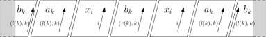
Figure 5: The unit 2-circular interval representation of $\overline{Subd_{2}(G)}$.

Note that this representation is almost the same as the unit 3-interval representation given for $\overline{Subd_{2}(G)}$ in the proof of Theorem 4.4, the only difference being that $I_{1}(b_{k})$ and $I_{3}(b_{k})$ have now been fused to form $I_{1}(b_{k})$ of the unit 2-circular interval representation being constructed. This representation can be constructed in linear time and it is easy to verify that the arcs have length $m^{2}$. Then one can also easily check in the figure that this is a valid unit 2-circular interval representation of $\overline{Subd_{2}(G)}$.  

4.6 2-circular track graphs

Theorem 4.8

Given any graph $G$, $\overline{Subd_{2}(G)}$ is a 2-circular track graph and a 2-circular track representation for it can be constructed in linear time.

Proof

We define a 2-circular track representation using circles $C_{1}$ and $C_{2}$, each having circumference at least $3n+1$, and mappings $I_{1}$ and $I_{2}$ defined as follows (see also Figure 6).

$\begin{array}[]{lcl}I_{1}(x_{i})=[i,i+n]\\ I_{1}(a_{k})=[l(k)+n+1,l(k)+2n]\\ I_{1}(b_{k})=[l(k)+2n+1,r(k)-1]\\ I_{2}(x_{i})=[i,i+n]\\ I_{2}(b_{k})=[r(k)+n+1,r(k)+2n]\\ I_{2}(a_{k})=[r(k)+2n+1,l(k)-1]\end{array}$

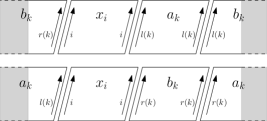
Figure 6: The 2-circular track representation of $\overline{Subd_{2}(G)}$.

Clearly, this representation can be constructed in linear time, and as before, it can be checked that the circles $C_{1}$ and $C_{2}$ together with the mappings $I_{1}$ and $I_{2}$ form a valid 2-circular track representation of $\overline{Subd_{2}(G)}$.  

5 NP-hardness in unit 2-interval and unit 3-track graphs

Valiant [25] has shown that every planar graph of degree at most 4 can be drawn on a grid of linear size such that the vertices are mapped to points of the grid and the edges to piecewise linear curves made up of horizontal and vertical line segments whose endpoints are also points of the grid. It is immediately clear that every planar graph $G$ has a subdivision $G^{\prime}$ that is an induced subgraph of a grid graph such that each edge of $G$ corresponds to a path of length at most $O(|V(G)|^{2})$ (see Figure 7). Note that here, some paths have even length and some have odd length. An even subdivision (resp. odd subdivision) of $G$ is a graph obtained from $G$ by subdividing each edge $e$ of $G$ an even (resp. odd) number of times, and at most $|V(G)|^{O(1)}$ times.

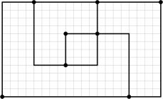
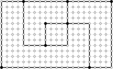
Figure 7: Embedding a planar graph in a grid.

Note that for any integer $k$, we can embed $G$ in a fine enough grid so that every horizontal and vertical segment in the original drawing of $G$ becomes a path that contains at least $k$ vertices in $G^{\prime}$. In Figure 7, we have chosen $k=5$.

Let $R(w,h)$ be the rectangular grid of height $h$ and width $w$. A path in $R(w,h)$ that contains only vertices from one row of the grid is called a horizontal grid-path and one that contains vertices from only one column is called a vertical grid-path. We denote by $R^{\prime}(w,h)$ the graph obtained by subdividing each edge of $R(w,h)$ once and by adding paths of length 3 between the newly introduced vertices as shown in Figure 8.

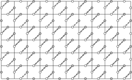
Figure 8: The graph $R^{\prime}(11,7)$. The vertices of the grid are not shown.

Lemma 1

Any planar graph $G$, on $n$ vertices and of maximum degree 4, has an even subdivision that is an induced subgraph of $R^{\prime}(w,h)$ for some values of $w$ and $h$ that are linear in $n$.

Proof

Let $H$ be the subdivision of $G$ that is an induced subgraph of the grid $R(w,h)$. Let $P_{e}$ denote the path in $H$ corresponding to an edge $e$ in $G$. We assume that $P_{e}$ is the union of horizontal and vertical grid-paths of length at least 5. We now transform the grid $R(w,h)$ into $R^{\prime}(w,h)$ by subdividing each edge once and by adding paths of length 3 between the newly introduced vertices as explained before. Clearly, a 1-subdivision of $H$, which we shall denote by $H^{\prime}$, is an induced subgraph of $R^{\prime}(w,h)$. It is also clear that $H^{\prime}$ is an odd subdivision of $G$. Let $P^{\prime}_{e}$ denote the path in $H^{\prime}$ corresponding to an edge $e$ of $G$. Note that $P^{\prime}_{e}$ consists of 1-subdivisions of vertical and horizontal grid-paths.

For every edge $e$ of $G$, we do the following procedure on $P^{\prime}_{e}$ in $H^{\prime}$ to obtain a new graph $H^{\prime\prime}$: we replace one of the subdivided horizontal or vertical grid-paths that make up $P^{\prime}_{e}$ to obtain $P^{\prime\prime}_{e}$ which has an even number of vertices as shown in Figure 9. The new graph $H^{\prime\prime}$ so obtained is an even subdivision of $G$ and is also an induced subgraph of $R^{\prime}(w,h)$.  

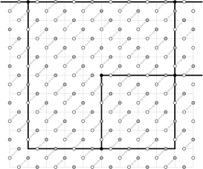
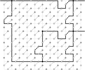
Figure 9: Modifying the paths in $H^{\prime}$ to obtain $H^{\prime\prime}$: A part of the graph in Figure 7 is shown. The grid vertices are not drawn.

Lemma 2

For any $w$ and $h$ the graph $\overline{R^{\prime}(w,h)}$ is both a unit 2-interval graph as well as a unit 3-track graph. Thus since those classes are closed under taking induced subgraphs, they also contain the induced subgraphs of $\overline{R^{\prime}(w,h)}$.

Proof

The graph $Q(w,l)$ is defined as follows. $V(Q(w,l))=X^{o}\cup X^{e}\cup A\cup B\cup C\cup D$ where $X^{o}=\{x^{o}_{1},\ldots,x^{o}_{w(l+1)}\}$, $X^{e}=\{x^{e}_{1},\ldots,x^{e}_{wl}\}$, $A=\{a_{1},\ldots,a_{2wl}\}$, $B=\{b_{1},\ldots,b_{2wl}\}$, $C=\{c_{1},\ldots,c_{2wl}\}$ and $D=\{d_{1},\ldots,d_{2wl}\}$.

$$E(Q(w,l)) = \bigcup_{i=1}^{wl}\{x^{o}_{i}a_{2i-1},x^{o}_{i}a_{2i}\}\cup\bigcup_{i=w+1}^{w(l+1)}\{x^{o}_{i}b_{2(i-w)-2},x^{o}_{i}b_{2(i-w)-1}\}$$

$$\cup\bigcup_{i=1}^{wl}\{x^{e}_{i}a_{2i-2},x^{e}_{i}a_{2i-1},x^{e}_{i}b_{2i-1},x^{e}_{i}b_{2i}\}$$

$$\cup\bigcup_{i=1}^{2wl-1}\{a_{i}c_{i},c_{i}d_{i},d_{i}b_{i+1}\}$$

Figure 10 shows a drawing of the graph $Q(w,l)$. The vertices in $(\bigcup_{i=1}^{l}\{a_{2wi},b_{2wi}\}\cup\bigcup_{i=1}^{2wl}\{c_{i},d_{i}\})$ are not shown to avoid clutter.

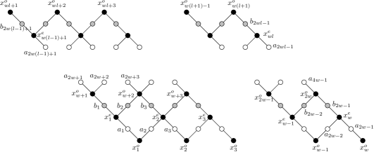
Figure 10: Part of the graph $Q(w,l)$.

It can be seen that $R^{\prime}(w,h)$ is an induced subgraph of $Q(w,\lceil\frac{w+h}{2}\rceil-1)$ (see Figure 11). Thus, to show that for any $w$ and $h$, $\overline{R^{\prime}(w,h)}$ is a unit 2-interval graph and a unit 3-track graph, we only need to show that $\overline{Q(w,l)}$ for any $w$ and $l$ is both a unit 2-interval graph as well as a unit 3-track graph.

Figure 11: $R^{\prime}(w,h)$ is an induced subgraph of $Q(w,l)$ where $l=\lceil\frac{w+h}{2}\rceil-1)$. The vertices in $(\bigcup_{i=1}^{l}\{a_{2wi},b_{2wi}\}\cup\bigcup_{i=1}^{2wl}\{c_{i},d_{i}\})$ are not shown.

We construct a unit 2-interval representation $f$ for $\overline{Q(w,l)}$ as follows (see also Figure 12).

$\begin{array}[]{lcl}I_{1}(a_{i})&=&[2i,2i+6n]\\ I_{1}(c_{i})&=&[2i+6n+2,2i+12n+2]\\ I_{1}(x^{o}_{i})&=&[4i+6n+1,4i+12n+1]\\ I_{2}(a_{i})&=&[2i+12n+4,2i+18n+4]\\ I_{1}(x^{e}_{i})&=&[4i+6n-1,4i+12n-1]\\ I_{1}(d_{i})&=&[2i,2i+6n]\\ I_{1}(b_{i})&=&[18n+6-2i,24n+6-2i]\\ I_{2}(d_{i})&=&[24n+6-2i,30n+6-2i]\\ I_{2}(b_{i})&=&[30n+10-2i,36n+10-2i]\\ I_{2}(x^{e}_{i})&=&[24n+9-4i,30n+9-4i]\\ I_{2}(x^{o}_{i})&=&[24n+11-4i+4w,30n+11-4i+4w]\\ I_{2}(c_{i})&=&[30n+8-2i,36n+8-2i]\end{array}$

Figure 12: Unit 2-interval representation of $\overline{Q(w,l)}$.

It is easy to verify that all the intervals have length $6n$. Then one can also check in the figure that this is a valid unit 2-interval representation of $\overline{Q(w,l)}$. Note that this construction is slightly more involved than the previous ones. Here the second blocks $x^{e}_{i}$ and $x^{o}_{i}$ are slightly shifted. This is due to the fact that $x^{e}_{i}$ is adjacent to every $b_{j}$, except $b_{i}$ and $b_{i+1}$, and that $x^{o}_{i}$ has to avoid a distinct $b$’s. Indeed $x^{o}_{i}$ is adjacent to every $b_{j}$, except $b_{i-w-1}$ and $b_{i-w}$. We construct now a unit 3-track representation for $\overline{Q(w,l)}$ as follows (see also Figure 13).

$\begin{array}[]{lcl}I_{1}(b_{i})&=&[i,i+2n]\\ I_{1}(x^{e}_{i})&=&[2i+2n+1,2i+4n+1]\\ I_{1}(x^{o}_{i})&=&[2i-2w+2n,2i-2w+4n]\\ I_{1}(a_{i})&=&[i+4n+4,i+6n+4]\\ I_{1}(c_{i})&=&[i+2n+3,i+4n+3]\\ I_{1}(d_{i})&=&[i+4n+4,i+6n+4]\\ I_{2}(a_{i})&=&[i,i+2n]\\ I_{2}(x^{e}_{i})&=&[2i+2n,2i+4n]\\ I_{2}(x^{o}_{i})&=&[2i+2n+1,2i+4n+1]\\ I_{2}(b_{i})&=&[i+2w+4n+4,i+2w+6n+4]\\ I_{2}(d_{i})&=&[i+2w+2n+4,i+2w+4n+4]\\ I_{2}(c_{i})&=&[i+2w+4n+5,i+2w+6n+5]\\ I_{3}(x^{o}_{i})&=&[2i,2i+4n]\\ I_{3}(a_{i})&=&[i+4n+2,i+8n+2]\\ I_{3}(c_{i})&=&[i+8n+3,i+12n+3]\\ I_{3}(b_{i})&=&[8n+3-i,12n+3-i]\\ I_{3}(d_{i})&=&[4n+1-i,8n+1-i]\\ I_{3}(x^{e}_{i})&=&[12n+5-2i,16n+5-2i]\end{array}$

Figure 13: Unit 3-track representation of $\overline{Q(w,l)}$.

It is easy to verify that all the intervals have length $4n$. Then one can also check in the figure that this is a valid unit 3-track representation of $\overline{Q(w,l)}$. Note that here also one has to be carefull with the $b_{i}$’s that $x^{e}_{i}$ and $x^{o}_{i}$ have to avoid.  

Theorem 5.1

MAXIMUM CLIQUE is NP-complete for unit 2-interval and unit 3-track graphs.

Proof

It is known that the MAXIMUM INDEPENDENT SET problem is NP-complete even when restricted to planar graphs of degree at most 3 [9]. It is folklore that the instance $(G,k)$ of MAXIMUM INDEPENDENT SET is equivalent to an instance $(H,k+k^{\prime})$, where $H$ is an even subdivision of $G$ with $|V(G)|+2k^{\prime}$ vertices. Thus according to Lemma 1, MAXIMUM INDEPENDENT SET is NP-complete on the class of induced subgraphs of $R^{\prime}(w,h)$. MAXIMUM CLIQUE is thus NP-complete on the class of induced subgraphs of $\overline{R^{\prime}(w,h)}$. Finally by Lemma 2 this class of graphs is contained in unit 2-interval and unit 3-track graphs. MAXIMUM CLIQUE is thus NP-complete on these classes.  

6 Complements of $t$-interval graphs

Very recently, Jiang and Zhang studied the class of complements of $t$-interval graphs [14]. In particular they proved that MINIMUM (INDEPENDENT) DOMINATING SET parameterized by the solution size is in W[1] for co-$2$-interval graphs, and they proved that MINIMUM DOMINATING SET is W[1]-hard for co-$3$-track graphs.

Following the same line of proof as for Theorem 4.2 we can prove the following APX-hardness results, for this kind of graph classes.

Theorem 6.1

  

• MINIMUM VERTEX COVER is APX-complete in co-2-interval graphs, and the complement classes of all the classes of Theorem 4.1.

• For any graph $G$, $Subd_{3}(G)$ is a co-2-interval, a co-unit-3-interval, a co-3-track, a co-unit-4-track, and a co-2-circular track graph, and MINIMUM (INDEPENDENT) DOMINATING SET is APX-hard for these classes of graphs.

Proof

The first item follows from the fact that MINIMUM VERTEX COVER is 2-approximable [20] and the first item of the following theorem.

Theorem 6.2 ([7])

• MINIMUM VERTEX COVER is APX-complete when restricted to $2k$-subdivisions of 3-regular graphs for any fixed integer $k\geq 0$.

• The problems MINIMUM DOMINATING SET, and MINIMUM INDEPENDENT DOMINATING SET are APX-complete when restricted to $3k$-subdivisions of degree at most 3 graphs for any fixed integer $k\geq 0$.

For the second item the constructions are described in the following figures. Here an edge $e_{k}=x_{i}x_{j}$ of $G$, with $i<j$, corresponds to a path $(x_{l(k)},a_{k},b_{k},c_{k},x_{r(k)})$ of $Subd_{3}(G)$. Then Theorem 6.2.(ii) clearly implies the APX-hardness.

Figure 14: The 2-interval representation of $\overline{Subd_{3}(G)}$.

Figure 15: The unit 3-interval representation of $\overline{Subd_{3}(G)}$.

Figure 16: The 3-track representation of $\overline{Subd_{3}(G)}$.

Figure 17: The unit 4-track representation of $\overline{Subd_{3}(G)}$.

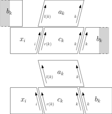
Figure 18: The 2-circular track representation of $\overline{Subd_{3}(G)}$.

 

7 Concluding remarks

The difference between the $4t$-approximation of Kammer et al. [16] and our $t$-approximation lies in two places. In their paper they proved that $t$-interval graphs are $2t$-perfectly orientable, but following the lines of Theorem 3.1 one can see that those graphs are $t$-perfectly orientable. This improves their approximation for MAXIMUM WEIGHTED INDEPENDENT SET, MINIMUM VERTEX COLORING, and MINIMUM CLIQUE PARTITION in $t$-interval graphs. For MAXIMUM WEIGHTED INDEPENDENT SET and MINIMUM VERTEX COLORING this reaches the best known ratio of $t$ [3] in a simpler way, and for the other problems it improves the best known approximation ratios [16]. Then Kammer et al. proved that MAXIMUM WEIGHTED CLIQUE can be $2k$-approximated in $k$-perfectly orientable graphs. Again, following the lines of Theorem 3.1 one can see that MAXIMUM WEIGHTED CLIQUE can be $k$-approximated for those graphs. This improves (by 2) their approximation for MAXIMUM WEIGHTED CLIQUE in $t$-fat objects intersection graphs.

In our approximation algorithm (as in the previous algorithms) we assume that we are given an interval representation. We wonder what we can do if we are not given such representation.

Open question. Can MAXIMUM (WEIGHTED) CLIQUE be polynomially $c(t)$-approximated in $t$-interval graphs, for some function $c$, if we are not given an interval representation?

This would be the case if there is an algorithm that computes, given a $t$-interval graph $G$, a $c(t)$-interval representation of $G$. Actually even when we are given a representation, the approximation ratio might be far from the optimal.

Open question. Does there exists an approximation algorithm for MAXIMUM (WEIGHTED) CLIQUE in $t$-interval graphs with a better approximation ratio?

Let us call $f(t)$ the better ratio a polynomial algorithm can achieve on $t$-interval graphs (actually $f(t)$ should be an infimum). For any graph $G$ on $n$ vertices, it is easy to construct a $n$-interval representation of $G$. Thus since for any $\epsilon>0$, one cannot $O(n^{1-\epsilon})$-approximate the MAXIMUM CLIQUE unless P = NP [27], we certainly have $f(t)=\Omega(t^{1-\epsilon})$.

The current status of the complexity of the MAXIMUM CLIQUE problem for the various classes of multiple interval graphs that were studied are shown in the table below (where “Unres.” stands for “Unrestricted”).

$t$	$t$-track		$t$-interval		Circular $t$-track		Circular $t$-interval
	Unit	Unres.	Unit	Unres.	Unit	Unres.	Unit	Unres.
1	P	P	P	P	P	P	P	P
2	P	P	NP-c	APX-c	?	APX-c	APX-c	APX-c
3	NP-c	APX-c	APX-c	APX-c	NP-c	APX-c	APX-c	APX-c
$\geq 4$	APX-c	APX-c	APX-c	APX-c	APX-c	APX-c	APX-c	APX-c

The blanks in this table clearly imply the following questions.

Open question. Is MAXIMUM CLIQUE for unit 2-interval graphs, unit 3-track graphs or unit 3-circular track graphs APX-hard, or does it admit a PTAS?

Open question. Is MAXIMUM CLIQUE for unit 2-circular track graphs Polynomial or NP-complete?

Koenig [17] explains that 2-track graphs have a polynomial-time algorithm for MAXIMUM CLIQUE because for any 2-track representation of a clique, there is a transversal of size 2 (i.e. two points such that for every vertex, at least one of its intervals contains one of these points). We note that this is not true for unit 2-circular track graphs as the complete graph on 5 vertices has a unit 2-circular track representation in which each circular track induces a cycle on 5 vertices. This representation clearly does not have a transversal of size 2.

References

- [1] Andrei Asinowski, Elad Cohen, Martin C. Golumbic, Vincent Limouzy, Marina Lipshteyn, and Michal Stern. Vertex Intersection Graphs of Paths on a Grid Journal of Graph Algorithms and Applications, 16 (2): 129–150, 2012.
- [2] Yonatan Aumann, Moshe Lewenstein, Oren Melamud, Ron Y. Pinter, and Zohar Yakhini. Dotted interval graphs and high throughput genotyping. In Proc. of the 16th Annual Symposium on Discrete Algorithms, SODA ’05, 339–348, 2005.
- [3] Reuven Bar-Yehuda, Magnús M. Halldórsson, Joseph S. Naor, Hadas Shachnai, and Irina Shapira. Scheduling split intervals. SIAM J. Comput. 36:1–15, 2006.
- [4] Piotr Berman, and Toshihiro Fujito. On approximation properties of the Independent set problem for degree 3 graphs. In Proceedings of the 4th Workshop on Algorithms and Data Structures, WADS ’95, LNCS Vol. 955, Springer-Verlag, pages 449–460, 1995.
- [5] Ayelet Butman, Danny Hermelin, Moshe Lewenstein, and Dror Rawitz. Optimization problems in multiple-interval graphs. In Proceedings of the eighteenth annual ACM-SIAM symposium on Discrete algorithms, SODA ’07, pages 268–277, 2007.
- [6] Sergio Cabello, Jean Cardinal, and Stefan Langerman. The Clique Problem in Ray Intersection Graph. arXiv http://arxiv.org/pdf/1111.5986.pdf, Nov. 2011.
- [7] Miroslav Chlebík and Janka Chlebíkova. The complexity of combinatorial optimization problems on -dimensional boxes. SIAM Journal on Discrete Mathematics, 21(1):158–169, 2007.
- [8] Maxime Crochemore, Danny Hermelin, Gad Landau, Dror Rawitz, and Stéphane Vialette. Approximating the 2-interval pattern problem. In Proc. of the 13th Annual European Symposium on Algorithms, ESA ’05, 426–437, 2005.
- [9] Michael R. Garey and David S. Johnson. Rectilinear steiner tree problem is NP-complete. SIAM J. Appl. Math. 6: 826–834, 1977.
- [10] Fanica Gavril. Algorithms for a maximum clique and a maximum independent set of a circle graph. Networks, 3: 261–273, 1973.
- [11] Fanica Gavril. Maximum weight independent sets and cliques in intersection graphs of filaments. Information Processing Letters, 73(5–6):181–188, 2000.
- [12] Dorit S. Hochbaum, and Asaf Levin. Cyclical scheduling and multi-shift scheduling: Complexity and approximation algorithms. Disc. Optimiz. 3(4):327–340, 2006.
- [13] Wen-Lian Hsu. Maximum weight clique algorithms for circular-arc graphs and circle graphs. SIAM J. Comput. 14(1):224–231, 1985.
- [14] Minghui Jiang and Yong Zhang Parameterized Complexity in Multiple-Interval Graphs: Domination, Partition, Separation, Irredundancy. arXiv, http://arxiv.org/pdf/1110.0187v1.pdf, Oct 2011.
- [15] Tomáš Kaiser. Transversals of d-Intervals. Discrete Comput Geom 18:195–203, 1997.
- [16] Frank Kammer, Torsten Tholey, and Heiko Voepel. Approximation algorithms for intersection graphs. In Proceedings of the 13th international workshop on Approximation Algorithms for Combinatorial Optimization Problems and 14th International workshop on Randomization and Computation, APPROX/RANDOM’10, pages 260–273, Berlin, Heidelberg, 2010. Springer-Verlag.
- [17] Felix G. König. Sorting with objectives. PhD thesis, Technische Universität Berlin, 2009.
- [18] Jan Kratochvíl and Jaroslav Nešetřil. Independent set and clique problems in intersection-defined classes of graphs. Commentationes Mathematicae Universitatis Carolinae, 31:85–93, 1990.
- [19] M. Middendorf and F. Pfeiffer. The max clique problem in classes of string-graphs. Discrete Mathematics, 108:365–372, 1992.
- [20] Burkhard Monien and Ewald Speckenmeyer. Ramsey numbers and an approximation algorithm for the vertex cover problem. Acta Inf. 22, 115–123, 1985.
- [21] Christos H. Papadimitriou, and Mihalis Yannakakis. Optimization, approximation, and complexity classes. J. Comput. System Sci. 43:425–440, 1991.
- [22] Edward R. Scheinerman. The maximum interval number of graphs with given genus. Journal of Graph Theory, 11(3):441–446, 1987.
- [23] Edward R. Scheinerman and Douglas B. West. The interval number of a planar graph: Three intervals suffice. Journal of Combinatorial Theory, Series B, 35(3):224–239, 1983.
- [24] William T. Trotter and Frank Harary. On double and multiple interval graphs. Journal of Graph Theory, 3(3):205–211, 1979.
- [25] Leslie G. Valiant. Universality considerations in VLSI circuits. IEEE Transactions on Computers, 30(2):135–140, 1981.
- [26] Douglas B. West and David B. Shmoys. Recognizing graphs with fixed interval number is NP-complete. Discrete Applied Mathematics, 8(3):295–305, 1984.
- [27] David Zuckerman. Linear degree extractors and the inapproximability of max clique and chromatic number. In Proc. 38th ACM Symp. Theory of Computing, STOC ’06, 681–690, 2006.