Non-adiabatic pumping in an oscillating-piston model

Abstract

We consider the prototypical “piston pump” operating on a ring, where a circulating current is induced by means of an AC driving. This can be regarded as a generalized Fermi-Ulam model, incorporating a finite-height moving wall (piston) and non trivial topology (ring). The amount of particles transported per cycle is determined by a layered structure of phase-space. Each layer is characterized by a different drift velocity. We discuss the differences compared with the adiabatic and Boltzmann pictures, and highlight the significance of the ”diabatic” contribution that might lead to a counter-stirring effect.

Stirring is the operation of inducing a DC circulating current by means of AC driving. This is naturally achieved by integrating a pump [1, 2, 3] in a closed circuit [4, 5]. It can also be regarded as a variation of a Hamiltonian ratchet [6, 7] where transport is induced in a periodic array. Pumping and stirring have largely been considered in the regime of slow (adiabatic) driving, where it can be related to the Berry phase that is associated with the driving cycle. This adiabatic approach is based on a simple picture of probability flow.

Challenging this oversimplified view, we argue that there are typical circumstances where the analysis should go beyond the adiabatic picture, even for very slow driving. We here present a detailed account of deterministic stirring that naturally extends into the non-adiabatic regime, complementary to related studies of stochastic stirring [8], Brownian ratchets [9], Brownian motors [10], stochastic [11] and chaotic [12] pumps.

We shall show that for a prototype system, the oscillating-piston model, even if the driving is very slow, the dynamics is actually complex, due to a non-trivial structure of phase-space, leading to drastic consequences for the transport.

1 Outline

After introducing the model, we describe the expectations that are based on a stochastic Boltzmann picture, and on a deterministic adiabatic picture. These suggest two different parametric results for the amount $Q$ of pumped particles. Then we present a proper analysis of the mixed phase-space dynamics, and highlight the limitations of the traditional reasoning.

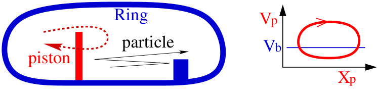
Figure 1: (Color on-line) An oscillating piston pump is integrated into a ring. The pumping cycle is illustrated on the right. The scattering within the ring is modeled as a potential barrier. We are considering a closed geometry that can be regarded a generalization of the Fermi-Ulam model. If we considered an open geometry, the pumping device would be connected between two unbiased reservoirs (not presented).

2 The model

We consider the prototype system illustrated in Fig.​​ 1: A particle with mass $\mathsf{m}$ moves in a ring of length $L$. There is a fixed barrier $V_{b}$ at $x{=}0$ and a moving wall (piston) of height $V_{p}$ at $x{=}X_{p}$. In the oscillating piston paradigm [3, 13], the two control parameters of the piston are cycled periodically through a closed loop in parameter space. The pumping cycle $(X_{p}(\varphi),V_{p}(\varphi))$, with $\varphi=\Omega t$, consists of translating the piston some distance to the right, shrinking its “height”, pulling it back to the left, and restoring its original “height”. In the sequel, we shall assume a harmonic driving with phase shift $\pi/2$ between the two parameters,

$$X_{p}(\varphi)\ = \ X_{0}-\delta X_{p}\cos(\varphi),$$ (1)

$$V_{p}(\varphi)\ = \ V_{p}+\delta V_{p}\sin(\varphi).$$ (2)

The velocity $v$ of the particle in dimensionless units is defined as ${u=v/(\delta X_{p}\Omega)}$. With the same convention the piston velocity $\dot{X_{p}}$ is expressed as ${u_{x}(\varphi)=\sin(\varphi)}$. The transmissions of the barrier and the piston are given by boolean expressions (true=1, false=0):

$$g_{b}(u)\ = \ \Big{[}|u|>u_{b}\Big{]},$$ (3)

$$g_{p}(u,\varphi)\ = \ \Big{[}|u{-}u_{x}(\varphi)|>u_{p}(\varphi)\Big{]},$$ (4)

where $u_{b,p}=[2V_{b,p}/\mathsf{m}]^{1/2}/(\delta X_{p}\Omega)$. In addition to the three dimensionless parameters ${(u_{b},u_{p},\delta u_{p})}$ that describe the barrier and the piston, we specify the geometry of the system defining $2\pi\ell_{+}\equiv X_{0}/\delta X_{p}$ and $2\pi\ell_{-}\equiv(L{-}X_{0})/\delta X_{p}$. A Poincaré section of the dynamics is obtained by taking snapshots of $(\varphi,u)$ after each collision with the fixed barrier:

$$\varphi_{n}^{\prime} = \varphi_{n}+\frac{2\pi\ell_{n}}{|u_{n}|},$$ (5)

$$u_{n}^{\prime} = -u_{n}+2u_{x}(\varphi_{n}^{\prime}),\ \ \ \mbox{if}\ g_{p}(u_{n},\varphi_{n}^{\prime}){=}0,$$ (6)

$$\varphi_{n+1} = \varphi_{n}^{\prime}+\frac{2\pi\ell_{n}^{\prime}}{|u_{n}^{\prime}|},$$ (7)

$$u_{n+1} = -u_{n}^{\prime},\ \ \ \mbox{if}\ g_{b}(u_{n}^{\prime}){=}0.$$ (8)

Above $\ell_{n}$ ($\ell_{n}^{\prime}$) is the scaled travel distance from the barrier to the piston (from the piston to the barrier). In the “static-wall approximation” it is $\ell_{+}$ or $\ell_{-}$ depending on the sign of $u_{n}$, while in the simulations the exact value can be numerically determined.

3 Objective

The map above generalizes the Fermi-Ulam model (FUM) [14]: here we have finite heights of piston and barrier, and periodic boundary conditions. Furthermore, while the FUM has been conceived to study energy absorption due to deterministic diffusion in momentum, here our interest is in the directed transport along the spatial coordinate. The amount of particles that are pumped per cycle is:

$$Q\ =\ \oint I{\rm d}t\ =\ \rho_{N}\left[\oint v(\varphi)\frac{{\rm d}\varphi}{2\pi}\right]\frac{2\pi}{\Omega},$$ (9)

where the current ${I\equiv\rho_{N}v(\varphi)}$ at a given moment of time is expressed by the spatial density of the particles $\rho_{N}$, and the drift velocity $v(\varphi)$. Assuming that a first-order description of adiabatic transport applies, if the piston is displaced with velocity $\dot{X}_{p}$, one expects a well defined induced current ${I=\mathcal{R}\rho_{N}\dot{X}_{p}}$, where $\mathcal{R}$ is an $\Omega$-independent dimensionless coefficient that primarily depends on $V_{p}$. One expects $\mathcal{R}\to 1$ for ${V_{p}\to\infty}$ and ${0<\mathcal{R}<1}$ for finite $V_{p}$. In such a case the amount of particles that are pumped per cycle becomes a parametric integral:

$$v(\varphi)=\mathcal{R}(\varphi)\ \dot{X}_{p}\ \ \ \leadsto\ \ \ Q=\rho_{N}\oint\mathcal{R}(\varphi){\rm d}X_{p}.$$ (10)

Below we try to formulate an adequate picture of the dynamics that interpolates between the opposite extremes of exclusively chaotic and purely regular motion. In particular: (i) we clarify what is the drift velocity for a general non-equilibrium steady state; (ii) we discuss whether a first-order description of adiabatic transport applies. We first review the common expectations.

(a)                                                                       (b)
      

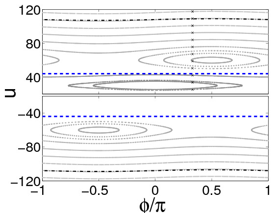
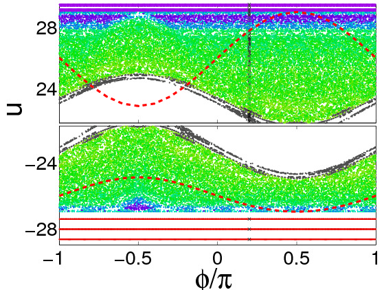
(c)                                                                       (d)
      

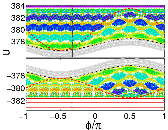
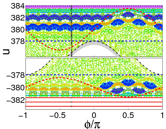
Figure 2: The $(\varphi,u)$ Poincaré section for a particle in a ring, with $l_{\pm}{=}15$, considering several cases: (a) ring with ${u_{p}{=}\infty}$ and ${u_{b}{=}44}$; (b) here ${u_{b}{=}0}$, and ${u_{p}{=}26}$, and ${\delta u_{p}{=}2.04}$; (c) here ${u_{b}{=}0}$, and ${u_{p}=380}$ and ${\delta u_{p}{=}2.55}$; (d) the same but with ${u_{b}{=}378}$. The color of each trajectory reflects its average drift velocity $\langle u\rangle$. Non transporting trajectories are colored gray. The dashed red lines indicate the piston scattering threshold $u^{\pm}(\varphi)$, while the dashed blue line gives that of the barrier $u_{b}$. The dot-dashed black lines are calculated adiabatic trajectories. Above the barrier the variation in $|u|$, due to the bounces with the piston, is $\sin(\varphi)$, with alternating sign in each bounce. Below the barrier $u$ keeps its sign, and the adiabatic variation is $[\langle|u|\rangle/(2\pi l_{+})]\cos(\varphi)$. See the appendix for details regarding the adiabatic trajectories.

4 The stochastic Boltzmann picture

The piston stirring problem has been analyzed in the past [13] using a stochastic approach with transmissions ${0<g_{b},g_{p}<1}$. Motivated by the prevailing literature that focuses on electronic systems one assumes a Fermi-like energy distribution, such that the initial occupation is

$$f(x,p) = \frac{1}{2\pi\hbar},\ \ \ \ \ \ \mbox{for $|p|<\mathsf{m}v_{\mbox{\tiny F}}$}$$ (11)

$$\rho_{N} = \frac{\mathsf{m}v_{\mbox{\tiny F}}}{\pi\hbar},\ \ \ \ \ \ \mbox{[density of particles]}$$ (12)

where $\mathsf{m}v_{\mbox{\tiny F}}$ is the Fermi momentum. In a classical context, $\hbar$ can be regarded as a parameter that determines the occupation density. Of interest is $f(p)=f(0,p)$, the momentum distribution at a section ${x=0}$ through which the current is measured. Its integral over ${\rm d}p$ gives the density of particles $\rho_{N}$. If ${|\dot{X}_{p}|\ll v_{\mbox{\tiny F}}}$, the momentum exchange due to collisions with the piston affects only a narrow shell of width $\sim 2\mathsf{m}\dot{X}_{p}$ around the Fermi energy ${E_{\mbox{\tiny F}}}$. Accordingly one writes

$$I\ =\ \int_{0}^{\infty}{\rm d}p[f(p)-f(-p)]v(p)\ =\ \rho_{N}\ \mathcal{R}\dot{X}_{p}.$$ (13)

From here Eq.​​ (10) is implied, while $\mathcal{R}$ is related to the reflectivity of the piston as follows [13]:

$$\mathcal{R}(\varphi)\ \ =\ \ \frac{(1-g_{p})\ g_{b}}{g_{p}+g_{b}-2g_{p}g_{b}}.$$ (14)

In the absence of a barrier (${g_{b}=1}$) the result is ${\mathcal{R}=1}$. If the ring is like a reservoir (${g_{b}=1/2}$) one observes that $\mathcal{R}=1{-}g_{p}$ is the reflectivity of the piston. The latter result is very well known [3], conventionally derived using the scattering formalism [1, 2].

5 Deterministic adiabatic picture

In our model the transmission coefficients of the barrier are given by Eqs.(3-4). In Eq.​​ (14) we have to substitute the values at the Fermi energy ${E_{\mbox{\tiny F}}=(1/2)\mathsf{m}v_{\mbox{\tiny F}}^{2}}$, which gives ${\mathcal{R}(\varphi)=\{0\,\mbox{or}\,1\}}$ depending on whether the piston is “below” or “above” the Fermi energy. In the latter case, from Eq.​​ (10) with Eq.​​ (12), we get ${dQ=[{\mathsf{m}v_{\mbox{\tiny F}}}/{\pi\hbar}]{\rm d}X_{p}}$, which coincides with [3]. If the Fermi energy is “above” the piston during the whole cycle, meaning that ${V_{p}(\varphi)<E_{\mbox{\tiny F}}}$ for any $\varphi$, we find ${Q=0}$. However, in the latter case, there is a naive (wrong) picture that suggests a finite result: Assuming that $Q$ is determined by the fraction of particles that are affected by the motion of the piston, the effective Fermi energy is $V_{p}(\varphi)$, and hence

$$Q\ =\ \frac{1}{\pi\hbar}\oint\sqrt{2\mathsf{m}V_{p}(\varphi)}\ {\rm d}X_{p}.$$ (15)

This “area” that is enclosed by the cycle resembles the action integral that is encountered in the canonical adiabatic picture. It has the form of Eq.​​ (10) with a modified ‘reflection’ coefficient ${\mathcal{R}(\varphi)=[V_{p}(\varphi)/E_{\mbox{\tiny F}}]^{1/2}}$. In spite of the wrong reasoning, Eq.​​ (15) is interesting because it can be justified as an approximation to what we call later “adiabatic contribution”.

6 Non-adiabatic deterministic dynamics

The Poincaré section for the generalized FUM Eqs.(5-8) is illustrated in Fig.​​ 2. We indicate there (by dashed red lines) the threshold velocity for piston reflection

$$u_{p}^{\pm}(\varphi)\ \ =\ \ u_{x}(\varphi)\pm u_{p}(\varphi)$$ (16)

which is implied by Eq.​​ (4). We define $v^{(\pm)}$ as the velocities that correspond to $\max[u_{p}^{+}]$ and $\min[u_{p}^{-}]$, respectively, and denote by $E^{(\pm)}$ the associated kinetic energies. For simplicity of presentation we assume that $V_{b}$ is smaller than $E^{(-)}$, which is always smaller than $E^{(+)}$. Accordingly, the ballistic motion of clockwise moving particle is not affected if ${E>E^{(-)}}$, while for anticlockwise moving particles the condition is ${E>E^{(+)}}$.

The non-integrable region in phase-space occupies the rectangular strip ${[v^{(-)},v^{(+)}]}$. One expects adiabatic dynamics if the slowness condition $|u|\gg\ell$ is satisfied there. Looking at Fig.​​ 2cd one observes that this region consists of layers. In each layer the motion is chaotic, with the possible exception of regular motion in some small islands. The lower layers, labeled collectively as ${r=0}$, are non-transporting: either the particle is bounded in the $\ell_{+}$ or in the $\ell_{-}$ segment, or else it occupies the whole ring without being ever able to cross one of the barriers. The motion in the subsequent transporting layers, labeled ${r=1,2,...r_{c}}$, is characterized by a non-zero drift velocity

$$\langle v\rangle_{r}\ \ \equiv\ \ \bar{u}_{r}\ \Omega\ \delta X_{p}$$ (17)

7 Stirring

Define $E^{(0)}$ as the minimal energy required for transporting motion. Consider a zero temperature Fermi occupation as the preparation. If either ${E_{\mbox{\tiny F}}}$ is below ${E^{(0)}}$ or above ${E^{(+)}}$ the induced current would be zero. In the latter case the non-regular transporting motion is merely a “musical chair” dynamics that takes place deep in the Fermi sea. The current would be non-zero if ${E^{(0)}<E_{\mbox{\tiny F}}<E^{(+)}}$, meaning that only a fraction of the transporting region is occupied. The amount of particles that are pumped during a period is ${Q=(2\pi/\Omega)\rho_{N}\langle v\rangle}$, where the cycle-averaged drift velocity is

$$\langle v\rangle\ =\ \sum_{r=1}^{r_{c}}f_{r}\langle v\rangle_{r}\ =\ \left[\sum_{r=1}^{r_{c}}f_{r}\bar{u}_{r}\right]\ \Omega\delta X_{p}$$ (18)

The normalized occupations satisfy $\sum f_{r}=1$, where ${r=0,1,2,...,r_{c}}$. For a saturated occupation the $f_{r}$ are proportional to the phase-space area of the filled layers. In the latter case $\langle v\rangle$ is merely the average velocity within the occupied region. If the whole transporting region is saturated, one obtains

$$\langle v\rangle\ =\ \frac{1}{2}\left(|v^{(+)}|-|v^{(-)}|\right)\ =\ \dot{X}_{p}$$ (19)

It should be realized that the dimensionless amplitude of the piston velocity is unity. Accordingly the condition for the emergence of multiple transporting layers is ${\delta u_{p}>2}$. Numerical results for $\langle v\rangle_{r}$ are presented in Fig.​​ 3b, and additional plots are available in Fig.​​ 4. Typically $\langle v\rangle_{r}$ is dominated by the the contribution that comes from the free ballistic stage of the motion. This contribution can be estimated quite easily (see below).

8 The drift velocity

At this stage we have to clarify how the drift velocities $\langle v\rangle_{r}$ are determined by the dynamics. The winding number (WN) of a trajectory that is generated by Eqs.(5-8), and its duration, are respectively

$$\mbox{WN}=\sum_{n}g_{b}(v_{n})\mbox{sign}(v_{n}),\ \ \ \ \ \mbox{Time}=\sum_{n}\frac{L}{|v_{n}|}$$ (20)

The drift velocity is

$$\bar{v} = \frac{\mbox{WN}}{\mbox{Time}}L=\frac{\sum_{n}g_{b}(v_{n})\mbox{sign}(v_{n})}{\sum_{n}|v_{n}|^{-1}}$$ (21)

$$= {\overline{g_{b}(v_{n})\mbox{sign}(v_{n})}}\ \Big{/}\ {\overline{|v_{n}|^{-1}}}$$

Using ergodicity the time average can be replaced by phase-space average. We just have to remember that $\varphi$ is like time, which is canonically conjugate to the energy. Hence the integration measure in phase-space is $\propto v{\rm d}v{\rm d}\varphi$. Consequently we get the obvious result

$$\bar{v}\ =\ \frac{\iint g_{b}(v)\,v\,{\rm d}v{\rm d}\varphi}{\iint{\rm d}v{\rm d}\varphi}\ \equiv\ \int v(\varphi)\frac{{\rm d}\varphi}{2\pi}$$ (22)

where the phase-space integration extends over the layer that is filled by the trajectory, and $v(\varphi)$ is defined as the parametric drift velocity. Results for the drift velocity are presented in Fig.​​ 3a.

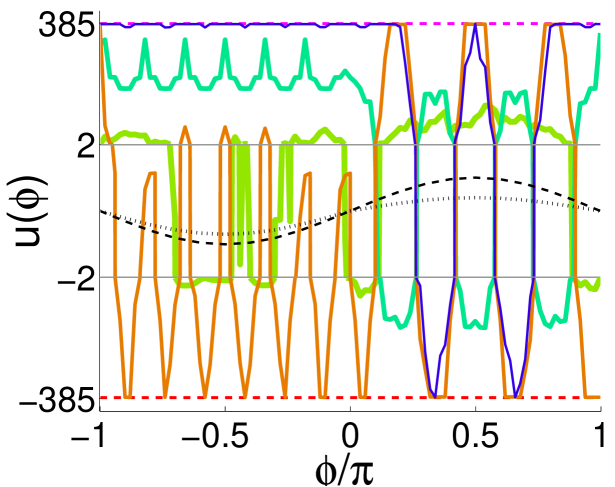
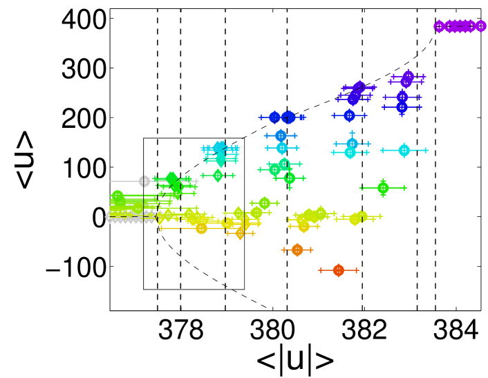
Figure 3: (Upper panel)  The drift velocity $u(\varphi)$ for trajectories in 4 representative layers (blue, cyan, orange, green) of Fig.​​ 2d. The motion consists of “free” and “adiabatic” stages. If the strict adiabatic picture were applicable it would be described by an expression $\mathcal{R}(\varphi)\dot{X}_{p}(\varphi)$, with ${0<\mathcal{R}(\varphi)<1}$, as illustrated by the dotted curve. The dashed curve is $\dot{X}(\varphi)$. The dashed horizontal lines correspond to $v^{(\pm)}$. Note that the ${[-2,+2]}$ range of the vertical axis is zoomed. (Lower panel)  The drift velocity $\left\langle{u}\right\rangle$ as function of $\langle|u|\rangle$, for the various layers that appear in Fig.​​ 2d (diamonds). One should exclude the framed data which represent additional layers that appear in Fig.​​ 2c (circles). The dashed black line assumes ${u>0}$ motion during the ballistic stage (see appendix), while the vertical dotted lines correspond to values of $u$ that accommodate an even number of bounces.

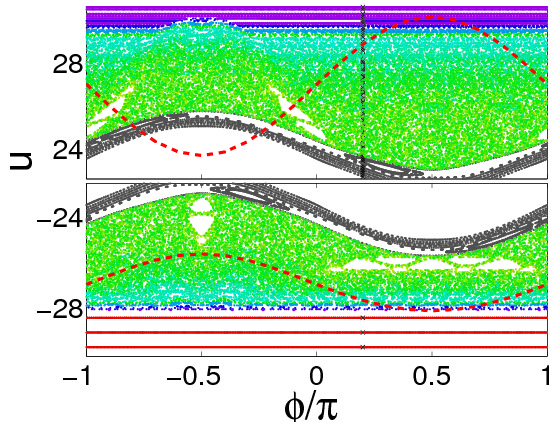
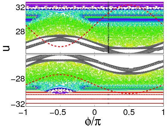
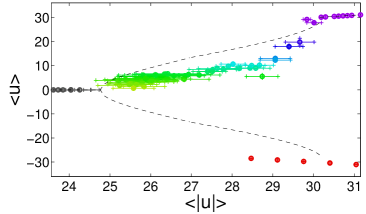
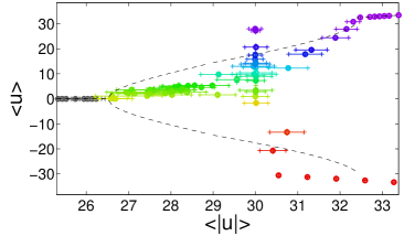
Figure 4: Additional Poincaré sections (top) showing mixed phase space. There is no barrier. The parameters are $l_{\pm}=15$, while ${u_{p}=27}$ (left) and ${u_{p}=29}$ (right) with ${\delta u_{p}=2.24,2.48}$, respectively. The color code and lines are as in Fig.​​ 2b. Corresponding plots of $\left\langle{u}\right\rangle$ in the bottom panels are as in Fig.​​ 3.

9 Estimate of the ‘free’ contribution

(can be skipped in first reading). Looking in Fig.​​ 2c we observe that in the absence of a barrier the motion in the transporting layers is not strictly adiabatic. Rather it contains a “diabatic transition” from adiabatic to free motion when $g_{p}$ switches from $0$ to $1$. For ${u>0}$ this transition takes place at the intersection of the stochastic layer with ${u^{+}(\varphi)}$. The relative filling of the ${u<0}$ branch is determined by the number of bounces that are accommodated in the adiabatic stage. It follows that the dependence of the drift velocity on $\langle|u|\rangle$ is modulated as seen in Fig.​​ 3b.

Neglecting small uncertainty of order $\dot{X}/v$, the ballistic motion takes place in the $\Delta\varphi$ interval where ${|u|>u_{p}(\varphi)}$. Hence this interval is determined by the roots of the equation ${u_{p}+\delta u_{p}\sin(\varphi)=|u|}$. Assuming that the ballistic motion takes place in the $u>0$ region of phase-space, without branching to the $u<0$ region, we get the upper bound estimate

$$\langle u\rangle_{r} = \left\langle\left|u\right|\right\rangle\left(\frac{\Delta\varphi}{2\pi}\right)$$ (23)

An improved estimate should take the branching into account. This branching depends on the number of bounces that are accommodated in the adiabatic stage. i.e. during the interval ${\Delta\varphi_{c}=2\pi-\Delta\varphi}$. The variation of $\varphi$ between successive bounces and the number of accommodated bounces are respectively

$$\Delta\varphi_{0}=\frac{2\pi\ell}{\left\langle\left|u\right|\right\rangle},\ \ \ \ \ \ m_{\mbox{\tiny bounces}}=\frac{\Delta\varphi_{c}}{\Delta\varphi_{0}}$$ (24)

We expect the branching to become negligible each time that $m$ crosses an even integer number. This in confirmed by the numerical results of Fig.​​ 3b.

10 Discussion of the adiabatic picture

Canonical adiabatic theory [15] ensures the invariance of the actions for a sufficiently slow perturbation of an otherwise integrable system. It is analogous to the conservation of the energy-level-index in its quantum version [16]. It holds as long as the trajectory does not change its topology. If a trajectory does change its topology, we call this occurrence a diabatic transition.

In the oscillating-piston model, each time that the motion switches between free ballistic motion, extended adiabatic motion, and bounded adiabatic motion, it is a diabatic transition. The two types of adiabatic motions are described in the appendix.

The small parameter of the adiabatic theory is $\dot{X}$. In the absence of magnetic field the zero-order adiabatic states carry no current. This is true both classically and quantum mechanically: note that in the latter case the parametric eigen-function ${|X\rangle}$ is real. It follows that adiabatic transport requires to go beyond zero-order. Linear response theory is based on a first-order treatment, leading to the Kubo formula for the transport coefficient. In open geometry the scattering formalism leads to the same result.

Using a quantum language, but referring on equal footing to the classical picture, the evolving zero-order adiabatic state ${|X(t)\rangle}$ does not satisfy the continuity equation: at any moment ${\langle I\rangle=0}$. Still we can deduce from the zero-order parametric solution a non-zero result for the current. This is done by associating a parametric velocity to each “piece” of the evolving probability distribution. This leads to Eq.​​ (15). We note that such procedure has been used in [17]. We also note that such procedure becomes ambiguous in the case of multiple path geometry: to associate a “displacement velocity” to each piece in phase space is not always well defined.

11 Contrasting with adiabaticity

The observed results imply that even for very slow driving the analysis should go beyond the adiabatic picture. If a first-order adiabatic transport picture were applicable, the drift velocity of the particle would adjust itself to the motion of the piston, and it would be possible to write Eq.​​ (10) with an $\Omega$-independent ${\mathcal{R}}$. In practice we observe that $\langle v\rangle_{r}$ has no simple linear relation to $\dot{X}_{p}$. The deterministic adiabatic result Eq.​​ (15) would be obtained if we had a saturated occupation of the region bounded by $u_{p}^{\pm}(\varphi)$. It can be regarded as a rough approximation to the total adiabatic contribution that we discuss below.

We already pointed out that the value of $\langle v\rangle_{r}$ within a layer of phase space is a sum of adiabatic-like and free ballistic contributions. The adiabatic-like contribution is proportional to the integral over $\dot{X}_{p}$ during the ${g_{p}=0}$ stage. The free ballistic contribution is due to the average velocity in the ${g_{p}=1}$ stage, during which the particle circulates the ring without being back-scattered. The result of the free ballistic contribution depends on the branching that has been explained previously, and accordingly, due to the alternating branching ratio, we observe an alternating net result for $\langle v\rangle_{r}$ as we go from layer to layer (Fig.​​ 3).

With a barrier the motion is somewhat more chaotic, and the local drift velocity adjusts better to $\dot{X}$, as seen in Fig.​​ 3a. A strict adiabatic approximation would be applicable if the momentary motion (for a frozen piston position) were chaotic, with some finite correlation time $\tau_{cl}$. Then the adiabatic condition would be $\Omega\tau_{cl}\ll 1$. This would require to consider a 2D ring, say a Sinai billiard. Within this approximation we could define $\mathcal{R}(\varphi)$ such that Eq.​​ (10) would lead to an $\Omega$ free parametric integral for $Q$.

12 Contrasting with Boltzmann

There are two conspicuous differences between our results and the expectations on the basis of the Boltzmann picture.  (a) In the Boltzmann picture, with “high” piston, in the absence of a barrier, we expect parametric transport with $\mathcal{R}=1$, hence obtaining $Q=0$ upon integration, implying zero drift velocity.  (b) Including a barrier, the Boltzmann picture suggests a non-zero net transport in the same direction that is implied by the pumping operation, with ${0<\mathcal{R}(\varphi)<1}$. This means ${\bar{u}_{r}>0}$ for all the layers. Both (a) and (b) are in contradiction to what we observe. In particular we point out that the negative $\bar{u}_{r}$ characterizing some of the layers is due to the possibility of having a free ballistic contribution with branching ratio that favors ${u<0}$ motion.

One should appreciate the essential difference between the Boltzmann and adiabatic pictures: Both would agree qualitatively if during the time of ${g_{p}=1}$ the drift velocity were zero. Instead it remains constant. One realizes that there is an “order of limits” issue: the Boltzmann picture assumes that there is always some infinitesimal reflection that allows in the adiabatic limit a randomization of the velocity. In contrast to that in the adiabatic picture the reflection during the ${g_{p}=1}$ stage is strictly zero and hence ${\langle v\rangle}$ remains constant.

13 Summary and discussion

A phase-space based approach for the analysis of stirring in a deterministic driven system has been presented. Our oscillating-piston model exhibits a layered mixed phase-space structure. The determination of the drift velocity requires to go beyond a simple parametric theory: in general neither an adiabatic nor a Boltzmann picture applies. The drift velocity in some layers can even have a sign opposite to the current direction that would be expected for a strictly adiabatic pumping (“counter stirring”). These chaotic layers appear already for slow driving, whereas a homogeneously chaotic phase-space, compatible with a stochastic picture of stirring, requires a different limit. It is important to realize that no simple relation can be established between a stirring problem and its corresponding pumping problem (that is, the same driven potential in an open configuration). Different paradigms are involved.

A few words are in order regarding the quantum case [13]: In the quantum adiabatic limit $\mathcal{R}$ can be calculated using the Kubo formalism. It has a wide distribution, which is the “geometric conductance” analogue of universal conductance fluctuations (UCF). One can even observe a counter-stirring effect ($\mathcal{R}<0$) which would be impossible in the strict classical adiabatic picture. The manifestation of dynamical localization requires significantly longer time scale of coherence, as explained in Ref.[7] with regard to Hamiltonian ratchets.

14 Appendix: adiabatic trajectories

In this appendix we clarify what are the equations that describe adiabatic trajectories for the pertinent two types of motion of the Fermi-Ulam “box model” and its “ring model” variation.

Bounded adiabatic motion: Consider a particle that is moving back and forth in a Box of length $L$, between an infinite barrier and an oscillating piston. In the $n$th collision the change in its velocity is $-2\dot{X}(t_{n})$. Summing over collisions, approximating by an integral over ${\rm d}t/(2L/v_{E})$, one obtains ${v(t)=\mbox{const}-(v_{E}/L)X(t)}$, where the absolute value of the velocity $v_{E}=(2E/\mathsf{m})^{1/2}$ is assumed to be approximately constant. This implies that the equation of the adiabatic curve in the Poincaré section for this type of motion is

$$u(\varphi)\ =\ \mbox{const}+\frac{u_{E}}{2\pi\ell}\cos(\varphi)$$ (25)

Note that in our ring setting $\ell$ is $\ell_{+}$ or $\ell_{-}$ depending whether it is ${u>0}$ or ${u<0}$ trajectory.

Extended adiabatic motion: There is a similar derivation for a particle on a clean ring of length $L$. There is no barrier. The particle changes direction each time that it collides with the moving piston. Consequently $v(t)$ changes sign each period, and it is convenient to sum the increments pairwise. This leads, after an even number of collisions, to the obvious result ${v(t)=\mbox{const}+\dot{X}(t)}$. This implies that the equation of the adiabatic curve in the Poincaré section for this type of motion is

$$u(\varphi)\ =\ \mbox{const}+\sin(\varphi)$$ (26)

15 Acknowledgments

This research was supported by the Israel Science Foundation (grant No.29/11), and by the Deutsch-Israelische Projektkooperation (DIP).

References

- [1] M. Büttiker, H. Thomas, A. Prêtre, Z. Phys. B 94, 133 (1994).
- [2] P.W. Brouwer, Phys. Rev. B 58, 10135 (1998).
- [3] J.E. Avron, A. Elgart, G.M. Graf, L. Sadun, Phys. Rev. B 62, 10618 (2000).
- [4] D. Cohen, Phys. Rev. B 68, 155303 (2003). I. Sela and D. Cohen, J. Phys. A 39, 3575 (2006).
- [5] M. Moskalets, M. Büttiker, Phys. Rev. B 68, 161311 (2003).
- [6] H. Schanz, M.-F. Otto, R. Ketzmerick, T. Dittrich, Phys. Rev. Lett. 87, 070601 (2001). H. Schanz, T. Dittrich, R. Ketzmerick, Phys. Rev. E 71, 026228 (2005).
- [7] L. Hufnagel, R. Ketzmerick, M.-F. Otto, H. Schanz, Phys. Rev. Lett. 89, 154101 (2002).
- [8] S. Rahav, J. Horowitz, C. Jarzynski, Phys. Rev. Lett. 101, 140602 (2008).
- [9] P. Hänggi, Rev. Mod. Phys. 81, 387 (2009). M.O. Magnasco, Phys. Rev. Lett. 71, 1477 (1993).
- [10] R.D. Astumian, P. Hänggi, Phys. Today 55, 33 (2002).
- [11] R.D. Astumian, I. Derenyi, Phys. Rev. Lett. 86, 3859 (2001). R.D. Astumian, Ann. Rev. Biophys. 40, 289 (2011).
- [12] A. Castañeda, T. Dittrich, G. Sinuco, arXiv:1111.1653
- [13] D.Cohen, T. Kottos, H. Schanz, Phys. Rev. E 71 035202R (2005). G. Rosenberg, D. Cohen, J. Phys. A 39, 2287 (2006). I. Sela, D. Cohen, Phys. Rev. B 77, 245440 (2008).
- [14] M.A. Lieberman, A.J. Lichtenberg, Phys. Rev. A 5, 1852 (1972).
- [15] M.A. Lieberman, A.J. Lichtenberg, Regular and Chaotic Dynamics, 2nd ed., Springer (New York, 1992).
- [16] A. Messiah, Quantum Mechanics, North Holland (Amsterdam, 1961).
- [17] D. Andrae, I. Barth, T. Bredtmann, H.-C. Hege, J. Manz, F. Marquardt, and B. Paulus, J. Phys. Chem. B, 115, pp 5476 (2011).