Leptonic asymmetry of the sterile neutrino hadronic decays in the $\nu MSM$

Abstract

We consider the leptonic asymmetry generation in the $\nu MSM$ via hadronic decays of sterile neutrinos at $T\ll T_{EW}$, when the masses of two heavier sterile neutrinos are between $m_{\pi}$ and 2 GeV. The choice of upper mass bound is motivated by absence of direct experimental searches for singlet fermions with greater mass. We carried out computations at zero temperature and ignored the background effects. Combining constraints of sufficient value of the leptonic asymmetry for production of dark matter particles, condition for sterile neutrino to be out of thermal equilibrium and existing experimental data we conclude that it can be satisfied only for mass of heavier sterile neutrino in the range $1.4$ GeV $\lesssim M<2$ Gev and only for the case of normal hierarchy for active neutrino mass.

1 Introduction

The Standard Model (SM) is minimal relativistic field theory, which is able to explain almost all particle physics experimental data [1]. However, there are several observable facts, that cannot be explained in the SM frame. Firstly, the neutrinos of SM are strictly massless, that contradict to the experimental fact of the neutrinos oscillations [2, 3]. The second problem is the impossibility to explain the baryon asymmetry of the Universe (BAU) within the SM. Finally, the SM does not provide the dark matter (DM) candidate. Also the SM can not solve the strong CP problem in particle physics, the primordial perturbations problem and the horizon problem in cosmology, etc.

The solutions of the above mentioned problems of the SM require some new physics between the electroweak and the Planck scales. An important challenge for the theoretical physics is to see if it is possible to solve them using only the extensions of the SM below the electroweak scale [4].

The Neutrino Minimal Standard Model ($\nu MSM$) is an extension of the SM by three massive right-handed neutrinos (sterile neutrinos), which do not take part in the gauge interactions of the SM . The model was suggested by M. Shaposhnikov and T. Asaka [5, 6]. The masses of sterile neutrinos are predicted to be smaller than electroweak scale, and thus there is no new energy scale introduced in the theory. The parameters of the $\nu MSM$ can be chosen in order to explain simultaneously the masses of active neutrinos, the nature of DM, and BAU.

The lightest sterile neutrino (the mass is expected to be in the KeV range [4]) can be intensively produced in the early Universe and have cosmologically long life-time. So, it might be a viable DM candidate. The sufficient amount of this neutrinos can be generated through an efficient resonant mechanism proposed by Shi and Fuller [7].

In the $\nu MSM$ the required amount of the leptonic asymmetry (in accordance with Shi and Fuller mechanism) can be created due to decays of the two heavier sterile neutrinos. This particles are generated at temperature $T>T_{EW}$ and their masses are expected to be in range $m_{\pi}<M_{I}<T_{EW}$ [8], where $m_{\pi}$ is the pion mass and $M_{I}$ is the mass of $I$-sterile neutrino. The leptonic asymmetry at the temperature of the sphaleron freeze-out ($T\sim T_{EW}$) is related to the baryon asymmetry of the Universe. At temperature $T<T_{EW}$ the leptonic asymmetry from decays of heavier sterile neutrinos can not convert into the baryon asymmetry and is accumulated. As it was shown in [4, 9] the required amount of the leptonic asymmetry $\Delta=\Delta L/L=(n_{L}-n_{\bar{L}})/(n_{L}+n_{\bar{L}})$:

$$10^{-3}<\Delta<2/11$$ (1)

has to already exist in the Universe at the moment of the beginning of production of the DM particles (takes place at the temperature around 0.1 GeV).

We consider here the leptonic asymmetry generation at $T\ll T_{EW}$, when the masses of two heavier sterile neutrinos are between $m_{\pi}$ and 2 GeV. The motivation is following. The mass of heavier sterile neutrino can not be less then $m_{\pi}$ (the constraint is coming from accelerator experiments combined with Big Bang Nucleosynthesis (BBN) bounds [10, 11]) and there is no direct experimental searches for singlet fermions with mass more then 2 Gev [10].

Since the masses of active neutrinos in the $\nu MSM$ are produced by the ”see-saw”  mechanism [12] some constraints on the parameters of the $\nu MSM$ come from active neutrino parameters that can be found from the experiments on the neutrino oscillations. Namely, these are the mass squared differences of active neutrinos and the mixing angles. Until recently the mixing angle $\theta_{13}$ was supposed to have a close to zero value. But new observations indicated its essential difference from zero [13].

The aim of this work is to obtain constraints on the parameters of the $\nu MSM$ from the required amount of the leptonic asymmetry and cosmology conditions. Also we want to investigate the influence of non-zero mixing angle $\theta_{13}$ on space of the allowed parameters of the $\nu MSM$. We do it following [14] using a simple model: we ignore the background effects and do computations at zero temperature.

The paper is organized as follows. In Section 2 we present the Lagrangian of the $\nu MSM$, make its convenient parametrization and present the Yukawa couplings in terms of active neutrinos mass matrix parameters. In Section 3 we derive the expression for the leptonic asymmetry. The limitations on the $\nu MSM$ parameters are imposed in Section 4. Section 5 is devoted to the analysis and conclusions.

2 Basic formalism of the $\nu MSM$

In the $\nu MSM$ [5, 6] the following terms are added to the Lagrangian of the SM (without taking into account the kinetic terms):

$$\mathcal{L}^{ad}=-F_{\alpha I}\bar{L}_{\alpha}\tilde{\Phi}\nu_{IR}-\frac{M_{IJ}}{2}\bar{\nu}_{IR}^{c}\nu_{JR}+h.c.,$$ (2)

where index $\alpha=e,\mu,\tau$ corresponds to the active neutrino flavors, indices $I,J$ run from $1$ to $3$, $L_{\alpha}$ is for the lepton doublet of the left-handed particles, $\nu_{IR}$ is for the field functions of the sterile right-handed neutrinos, the superscript $\raisebox{-8.00003pt}{$"$}\!c"$ means charge conjugation, $F_{\alpha I}$ is for the new (neutrino) matrix of the Yukawa constants, $M_{IJ}$ is for the Majorana mass matrix of the right-handed neutrinos, $\Phi$ is for the field of the Higgs doublet, ${\tilde{\Phi}}=i\sigma_{2}\Phi^{*}$.

After the spontaneous symmetry breaking the field of the Higgs doublet in unitary gauge is

$$\Phi=\left(\begin{array}[]{c}0\\ \frac{v+h}{\sqrt{2}}\end{array}\right),$$

where $h$ is the neutral Higgs field and the parameter $v$ determines minimum of the Higgs field potential $(v\cong 247\,\,\mbox{GeV})$. In this case Lagrangian (2) acquires the Dirac-Majorana neutrino mass terms:

$$\mathcal{L}^{DM}=-\frac{v}{\sqrt{2}}F_{\alpha I}\bar{\nu}_{\alpha}\nu_{IR}-\frac{M_{IJ}}{2}\bar{\nu}_{IR}^{c}\nu_{JR}+h.c.,$$ (3)

or in conventional form [15]

$$\mathcal{L}^{DM}=-\left(\overline{(N_{L})^{c}}\,\frac{M^{DM}}{2}\,N_{L}+h.c.\right),$$ (4)

where

$$N_{L}=\left(\begin{array}[]{c}\nu_{L}\\ \nu_{R}^{c}\\ \end{array}\right)\!;\,\,N_{L}^{c}=\left(\begin{array}[]{c}\nu_{L}^{c}\\ \nu_{R}\\ \end{array}\right)\!;\,\,M^{DM}=\left(\begin{array}[]{cc}M_{L}&M_{D}{}^{T}\\ M_{D}&M_{R}\\ \end{array}\right)\!$$ (5)

and

$$M_{L}=0,\quad M_{D}=F^{+}\frac{v}{\sqrt{2}}\,,\quad M_{R}=M^{*},$$ (6)

where $M,F$ are square matrix of the third order with elements $F_{\alpha I}$ and $M_{IJ}$.

In zero approximation the $\nu MSM$ Lagrangian is assumed to be invariant under $U(1)_{e}\times U(1)_{\mu}\times U(1)_{\tau}$ transformations, that provides preservation of the $e,\mu,\tau$ lepton numbers separately. It is also assumed that two heavier sterile neutrinos interact with the active neutrinos, but the third (lightest) sterile neutrino does not interact. This assumption can be realized by following matrix $M^{DM}$[16]:

$$M_{R}^{(0)}=\left(\begin{array}[]{ccc}0&0&0\\ 0&0&M\\ 0&M&0\end{array}\right),\qquad M_{D}^{(0)+}=\frac{v}{\sqrt{2}}\left(\begin{array}[]{ccc}0&h_{12}&0\\ 0&h_{22}&0\\ 0&h_{32}&0\end{array}\right),\qquad M_{L}^{(0)}=0$$ (7)

In this approximation we have two massive sterile neutrinos with equal mass $M$, the third neutrino is massless, and all active neutrinos have zero mass. It contradicts observable data [2, 3]. To adjust it next small terms are added to the matrix $M^{DM}$ [16]:

$$M_{R}^{(1)}=\Delta M=\left(\begin{array}[]{ccc}m_{11}e^{-i\alpha}&m_{12}&m_{13}\\ m_{12}&m_{22}e^{-i\beta}&0\\ m_{13}&0&m_{33}e^{-i\gamma}\end{array}\right),\\ M_{D}^{(1)+}=\frac{v}{\sqrt{2}}\left(\begin{array}[]{ccc}h_{11}&0&h_{13}\\ h_{21}&0&h_{23}\\ h_{31}&0&h_{33}\end{array}\right),M_{L}^{(1)}=0$$ (8)

This correction violates $U(1)_{e}\times U(1)_{\mu}\times U(1)_{\tau}$ symmetry, leads to the appearance of the mass of the third sterile neutrino and takes off the mass degeneracy for two heavier sterile neutrinos. It’s also leads to the appearance of the extra small masses of the active neutrinos and nonzero mixing angles among them.

In the terms of the introduced corrections Lagrangian (2) is

$$\mathcal{L}^{ad}=-h_{\alpha I}\bar{L}_{\alpha}\tilde{N_{I}}\tilde{\Phi}-M\bar{\tilde{N_{2}^{c}}}\tilde{N_{3}}-\frac{\Delta M_{IJ}}{2}\bar{\tilde{N_{I}^{c}}}\tilde{N_{J}}+h.c.,$$ (9)

where $\tilde{N_{I}}$ are right-handed neutrinos in the gauge basis.

In order to find the masses of the active neutrino one has to make the diagonalization of the matrix $M^{DM}$. The diagonalization undergoes in two steps. Firstly, $M^{DM}$ matrix is reduced to the block-diagonal form via the unitary transformation [17] in the ”see-saw”  approach:

$$M_{block}=W^{T}M^{DM}W=\left(\begin{array}[]{cc}-(M_{D})^{T}(M_{R})^{-1}M_{D}&0\\ 0&M_{R}\end{array}\right)=\left(\begin{array}[]{cc}M_{light}&0\\ 0&M_{heavy}\end{array}\right),$$ (10)

where

$$W=\left(\begin{array}[]{cc}1-\frac{1}{2}\varepsilon^{+}\varepsilon&\varepsilon^{+}\\ -\varepsilon&1-\frac{1}{2}\varepsilon\varepsilon^{+}\\ \end{array}\right),\quad\varepsilon=M_{R}^{-1}M_{D}\ll 1$$ (11)

and $M_{light}=-(M_{D})^{T}(M_{R})^{-1}M_{D}$, $M_{heavy}=M_{R}$ are the mass matrix of the active and sterile neutrinos respectively. Now each block of the matrix $M^{DM}$ may be diagonalized independently by the matrix

$$U=\left(\begin{array}[]{cc}U_{1}&0\\ 0&U_{2}\\ \end{array}\right).$$ (12)

The mass matrix of the active and sterile neutrinos is diagonalized by unitary transformation $U_{1(2)}$:

$$U_{1}^{T}M_{light}U_{1}=diag(m_{1},m_{2},m_{3}),\quad U_{2}^{T}M_{heavy}U_{2}=diag(M_{1},M_{2},M_{3}).$$ (13)

There is a standard parametrization [2] for $U_{1(2)}$:

$$U_{1(2)}=\left(\!\!\begin{array}[]{ccc}c_{12}c_{13}&c_{13}s_{12}&s_{13}e^{-i\delta}\\ -s_{12}c_{23}-c_{12}s_{23}s_{13}e^{i\delta}&c_{12}c_{23}-s_{12}s_{23}s_{13}e^{i\delta}&s_{23}c_{13}\\ s_{12}s_{23}-c_{12}c_{23}s_{13}e^{i\delta}&-c_{12}s_{23}-s_{12}c_{23}s_{13}e^{i\delta}&c_{23}c_{13}\\ \end{array}\!\!\right)\times\\ \times\left(\!\!\begin{array}[]{ccc}e^{i\alpha_{1}/2}&0&0\\ 0&e^{i\alpha_{2}/2}&0\\ 0&0&1\\ \end{array}\!\!\right)\!\!,$$ (14)

where $c_{ij}=\cos\theta_{ij}$, $s_{ij}=\sin\theta_{ij}$, $\theta_{12},\theta_{13},\theta_{23}$ are the three mixing angles; $\delta$ is the Dirac phase, and $\alpha_{1},\alpha_{2}$ are the Majorana phases. The angles $\theta_{ij}$ can be in the region $0\leq\theta_{ij}\leq\pi/2$, phases $\delta,\alpha_{1},\alpha_{2}$ vary from $0$ to $2\pi$. Each of the matrices $U_{1}$ and $U_{2}$ contains its own, independent angles and phases.

Then the elements of the $M_{light}$ can be defined by masses and elements of mixing matrix $U$ of the active neutrinos:

$$[M_{light}]_{\alpha\beta}=m_{1}U^{*}_{\alpha 1}U^{*}_{\beta 1}+m_{2}U^{*}_{\alpha 2}U^{*}_{\beta 2}+m_{3}U^{*}_{\alpha 3}U^{*}_{\beta 3}.$$ (15)

The data that come from the neutrino oscillation experiments are presented in Tab.1:

central value	99$\%$ confidence interval
$\Delta m^{2}_{21}=(7.58\pm 0.21)\cdot 10^{-5}\,eV^{2}$	$(7.1-8.1)\cdot 10^{-5}eV^{2}$
$|\Delta m^{2}_{23}|=(2.40\pm 0.15)\cdot 10^{-3}eV^{2}$	$(2.1-2.8)10^{-3}eV^{2}$
$tan^{2}\theta_{12}=0.484\pm 0.048$	$31^{0}<\theta_{12}<39^{0}$
$sin^{2}2\theta_{23}=1.02\pm 0.04$	$37^{0}<\theta_{23}<53^{0}$
${}^{*}\quad$ $\sin^{2}2\theta_{13}=0.11$ ($\theta_{13}=10^{0}$)

Table 1. Experimental constraints on the parameters of active neutrinos [3], ^∗ — results of T2K Collaboration [13]: $0.03<\sin^{2}2\theta_{13}<0.28$ in the case of the normal hierarchy and $0.04<\sin^{2}2\theta_{13}<0.34$ in the case of the inverted hierarchy.

sss

On the other hand, from the ”see-saw”  formula (in the approximation when the elements of the first column of the Yukawa matrix are neglected and $M\gg m_{ij}$) one can immediately obtain, that the mass of the lightest sterile neutrino is zero and the mass matrix of the active neutrinos has the form [16]

$$[M_{light}]_{\alpha\beta}=-\frac{v^{2}}{2M}(h_{\alpha 2}h_{\beta 3}+h_{\alpha 3}h_{\beta 2}),$$ (16)

and its eigenvalues is

$$m_{a}=0,\quad m_{\tiny\left(\!\!\!\begin{array}[]{c}b\\ c\end{array}\!\!\!\right)}=\frac{v^{2}(F_{2}F_{3}\mp|h^{+}h|_{23})}{2M},$$ (17)

where $F_{I}^{2}=(h^{+}h)_{II}$, $m_{a}$ is the mass of the lightest active neutrino, $m_{c}$ is the mass of the heaviest active neutrino. The sum over the neutrino masses is given by

$$\frac{v^{2}F_{2}F_{3}}{M}=\sum_{i=1}^{3}m_{i}.$$ (18)

The system (16) has infinite number of solutions. Indeed, the replacement $h_{\alpha 2}\rightarrow zh_{\alpha 2}$, $h_{\alpha 3}\rightarrow h_{\alpha 3}/{z}$ ($z$ is an arbitrary complex number) does not change the system. Then one can define the real quantity $\varepsilon$

$$\varepsilon={F_{3}}/{F_{2}},\quad\varepsilon=|z|.$$ (19)

as an independent parameter of the model.

As it was shown in [18], the system (16) has good solutions for ratios of the elements of second column of the Yukawa matrix:

$$\left\{\begin{array}[]{c}\vspace{0.5em}A_{12}=\displaystyle{\frac{M_{12}}{M_{22}}\left(1\pm\sqrt{1-\frac{M_{11}M_{22}}{M_{12}{}^{2}}}\right)}\\ \vspace{0.5em}A_{13}=\displaystyle{\frac{M_{13}}{M_{33}}\left(1\pm\sqrt{1-\frac{M_{11}M_{33}}{M_{13}{}^{2}}}\right)}\\ A_{23}=\displaystyle{\frac{M_{23}}{M_{33}}\left(1\pm\sqrt{1-\frac{M_{22}M_{33}}{M_{23}{}^{2}}}\right)}\end{array}\right.$$ (20)

where $A_{12}={h_{12}}/{h_{22}}$, $A_{13}={h_{12}}/{h_{32}}$, $A_{23}={h_{22}}/{h_{32}}$ and $M_{IJ}$ is elements of $M_{light}$ matrix. The ratios of the third column elements of the Yukawa matrix are expressed through the $A_{ij}$ elements:

$$\frac{h_{23}}{h_{13}}=A_{12}\frac{M_{22}}{M_{11}};\quad\frac{h_{33}}{h_{13}}=A_{13}\frac{M_{33}}{M_{11}}.$$ (21)

Though formally there are eight different choices for the solutions (20), only four are independent. For example, if we fix the sign before the square roots in the expressions for $A_{12}$ and $A_{13}$ then $A_{23}$ is unambiguously determined by the relation

$$A_{23}=A_{13}/A_{12}.$$ (22)

The solutions (20) allow one to find the ratios of the elements of Yukawa matrix [18]:

$$\frac{\left(h_{12};h_{22};h_{32}\right)}{F_{2}}=\frac{e^{iarg(h_{12})}}{\sqrt{1+|A_{12}|^{-2}+|A_{13}|^{-2}}}\left(1;A_{12}^{-1};A_{13}^{-1}\right)$$ (23)

$$\frac{\left(h_{13};h_{23};h_{33}\right)}{F_{3}}=\frac{e^{iarg(h_{13})}}{\sqrt{1+|A_{12}\frac{M_{22}}{M_{11}}|^{2}+|A_{13}\frac{M_{33}}{M_{11}}|^{2}}}\left(1;A_{12}\frac{M_{22}}{M_{11}};A_{13}\frac{M_{33}}{M_{11}}\right),$$ (24)

where phases of $h_{12}$, $h_{13}$ are connected by condition

$$arg(h_{12})+arg(h_{13})=arg(M_{11}).$$ (25)

This is the exact solution of (16) that definitely expresses ratio of the elements of the Yukawa matrix via parameters of the active neutrino mass matrix. For fixed values of the active neutrino parameters there are only two choices for placing of the signs in the expressions for $A_{12},A_{13},A_{23}$ (20) which are not inconsistent with condition (22). These two variants are distinguished from each other by simultaneous replacement of the sign in front of square roots in the expressions for $A_{12},A_{13},A_{23}$. It can be shown that such replacement of the signs leads to interchanging and conjugating of the ratios of elements of the second and the third columns of the Yukawa matrix, notably $h_{22}/h_{12}\leftrightarrow h^{*}_{23}/h^{*}_{13}$, $h_{32}/h_{12}\leftrightarrow h^{*}_{33}/h^{*}_{13}$ [18].

As it was announced in Introduction, only the two heavier sterile neutrino take part in the production of the leptonic asymmetry. Therefore we will exclude the lightest sterile neutrino from consideration, so hereinafter indexes $I,J$ take the value 2 or 3 referring to the two heavy sterile neutrinos. In this case there are 11 additional parameters in the $\nu MSM$ as compared with SM. Seven of them we will identify with the elements of the active neutrino mass matrix ($m_{2}$, $m_{3}$, $\theta_{12}$, $\theta_{13}$, $\theta_{23}$, $\delta$, $\alpha_{2}$). The other 4 we will define as follows: the average mass of two heavier sterile neutrinos $M=\frac{M_{2}+M_{3}}{2}$, their mass splitting $\Delta M=\frac{M_{3}-M_{2}}{2}$, the parameter $\varepsilon$ and the phase $\xi=arg(h_{12})$.

Thus, we can parameterize the Lagrangian (9) in the following way:

$$\mathcal{L}=\left(\frac{M\sum m_{\nu_{i}}}{v^{2}}\right)^{\frac{1}{2}}\left[\frac{1}{F_{2}\sqrt{\varepsilon}}h_{\alpha 2}\bar{L}_{\alpha}\tilde{N}_{\alpha}+\frac{\sqrt{\varepsilon}}{F_{3}}h_{\alpha 3}\bar{L}_{\alpha}\tilde{N}_{3}\right]\tilde{\Phi}-\\ -M\bar{\tilde{N}}_{2}^{c}\tilde{N}_{3}-\frac{1}{2}\Delta M\left(\bar{\tilde{N_{2}^{c}}}\tilde{N}_{2}+\bar{\tilde{N_{3}^{c}}}\tilde{N}_{3}\right)+h.c.,$$ (26)

where $a_{\alpha I}={h_{\alpha I}}/{F_{I}}$ are defined by equations (23) and (24).

Lagrangian (2) can be written in another basis, namely when the mass matrix of sterile right-handed neutrinos is diagonal. In this case the Lagrangian is

$$\mathcal{L}^{ad}=-g_{\alpha I}\bar{L}_{\alpha}{N^{\prime}_{I}}\tilde{\Phi}-\frac{M_{I}}{2}\bar{N}^{\prime}{}_{I}^{c}N^{\prime}_{I}+h.c.,$$ (27)

where ${N^{\prime}_{I}}$ are right-handed neutrinos and $g_{\alpha I}$ are elements of the Yukawa matrix in this basis.

Transition from presentation of Lagrangian (2) in gauge and mass basis can be made with unitary transformation that transfers mass matrix of right-handed neutrino to diagonal form [14, 16]:

$$V^{*}\left(\begin{array}[]{cc}\Delta M&M\\ M&\Delta M\end{array}\right)V=\left(\begin{array}[]{cc}M-\Delta M&0\\ 0&M+\Delta M\end{array}\right);\quad V=\frac{1}{\sqrt{2}}\left(\begin{array}[]{cc}-i&i\\ 1&1\end{array}\right).$$ (28)

So, the transition can be made by

$$\tilde{N}_{I}=V_{IJ}N^{\prime}{}_{J},\quad g_{\alpha I}=h_{\alpha J}V_{JI}.$$ (29)

With help of this relations it will be useful to express Lagrangian (26) in terms of right-handed neutrino functions of Lagrangian (27)

$$\mathcal{L}^{ad}=-\left(\frac{M\sum m_{\nu_{i}}}{2v^{2}}\right)^{\frac{1}{2}}\left[\left(\frac{ia_{\alpha 2}}{\sqrt{\varepsilon}}-i\sqrt{\varepsilon}a_{\alpha 3}\right)\bar{L}_{\alpha}N^{\prime}{}_{2}+\left(\frac{a_{\alpha 2}}{\sqrt{\varepsilon}}+\sqrt{\varepsilon}a_{\alpha 3}\right)\bar{L}_{\alpha}N^{\prime}{}_{3}\right]\tilde{\Phi}-\\ -\frac{1}{2}\left(M-\Delta M\right)\bar{{N^{\prime}{}_{2}^{c}}}N^{\prime}{}_{2}-\frac{1}{2}(M+\Delta M)\bar{{N^{\prime}{}_{3}^{c}}}N^{\prime}{}_{3}.$$ (30)

After comparing (30) and (27) one can express Yukawa couplings in different presentations

$$g_{\alpha 2}=\left(\frac{M\sum_{i}m_{\nu_{i}}}{2v^{2}}\right)^{\frac{1}{2}}\left(\frac{ia_{\alpha 2}}{\sqrt{\varepsilon}}-i\sqrt{\varepsilon}a_{\alpha 3}\right),$$ (31)

$$g_{\alpha 3}=\left(\frac{M\sum_{i}m_{\nu_{i}}}{2v^{2}}\right)^{\frac{1}{2}}\left(\frac{a_{\alpha 2}}{\sqrt{\varepsilon}}+\sqrt{\varepsilon}a_{\alpha 3}\right).$$ (32)

The mass eigenstates neutrinos for Lagrangian with the mass matrix $M^{DM}$ (5) can be easily expressed through the states of neutrino of Lagrangian (27), particularly:

$$N^{c}=\left(1-\frac{1}{2}\varepsilon\varepsilon^{+}\right)N^{\prime}{}^{c}+\varepsilon\nu_{L}\simeq N^{\prime}{}^{c}+\varepsilon\nu_{L},$$ (33)

where $N$ are mass eigenstates of the right-handed neutrinos in which they are produced and decay, $\nu_{L}$ are the active neutrinos of the SM in flavor basis,

$$\varepsilon_{\alpha I}\equiv\Theta_{\alpha I}=\frac{v}{\sqrt{2}}\frac{g_{\alpha I}}{M_{I}}$$ (34)

is the mixing angle ($\varepsilon_{\alpha I}\ll 1$).

3 The computation of the leptonic asymmetry.

             

As it was pointed in Section 1, leptonic asymmetry in the $\nu MSM$ is generated due to decays of the heavier sterile neutrinos on SM particles. At temperature $T\ll T_{EW}$ the interaction of the sterile neutrinos with SM particles via neutral Higgs field can be neglected. The only possible way of interaction of the sterile neutrino with matter is through the mixing with active neutrinos (33).

For the sterile neutrino with the mass $m_{\pi}<M_{I}<$ 2 GeV the channels for the decay into two-body final state are:

$$N_{I}\rightarrow\pi^{0}\nu_{\alpha},\pi^{+}e_{\alpha}^{-},\pi^{-}e_{\alpha}^{+},K^{+}e_{\alpha}^{-},K^{-}e_{\alpha}^{+},\eta\nu_{\alpha},\eta^{\prime}\nu_{\alpha},\rho^{0}\nu_{\alpha},\rho^{+}e_{\alpha}^{-},\rho^{-}e_{\alpha}^{+}.$$ (35)

The channel of decay $N_{2,{3}}\rightarrow N_{1}+...$ is strongly suppressed because of the small Yukawa coupling constants of $N_{1}$. The decay of the sterile neutrino into the $K^{0}$ state is forbidden, because the composition of $K^{0}$ ($d\bar{s}$) can not be obtained by decay of $Z$-boson.

The three-body final state can be safely neglected and also the many hadron final state [10]. This last decay channels contribute for less than 10% for $M_{I}<2$ GeV. For $m_{\pi}<M_{I}<2$ GeV the decays into D-meson can also be neglected because its mass is not much smaller than 2 GeV.

Let us consider the decay of the sterile neutrino in the $\nu MSM$. Sterile neutrino oscillates into active neutrino that decay into $Z$-bozon and active neutrino (or $W^{\pm}$-boson and charged lepton) in accordance with the SM. $Z$-boson (or $W^{\pm}$-boson) hereafter decays into quark-antiquark pair, see Fig.1. Since kinetic energy of this quarks are small enough the quark pair will form a bound state. Since $M_{I}<2$ GeV $\ll M_{Z(W)}$ we can use low energy Fermi theory and shrink the heavy boson propagator into an effective vertex and use for final state a meson, see Fig.2.

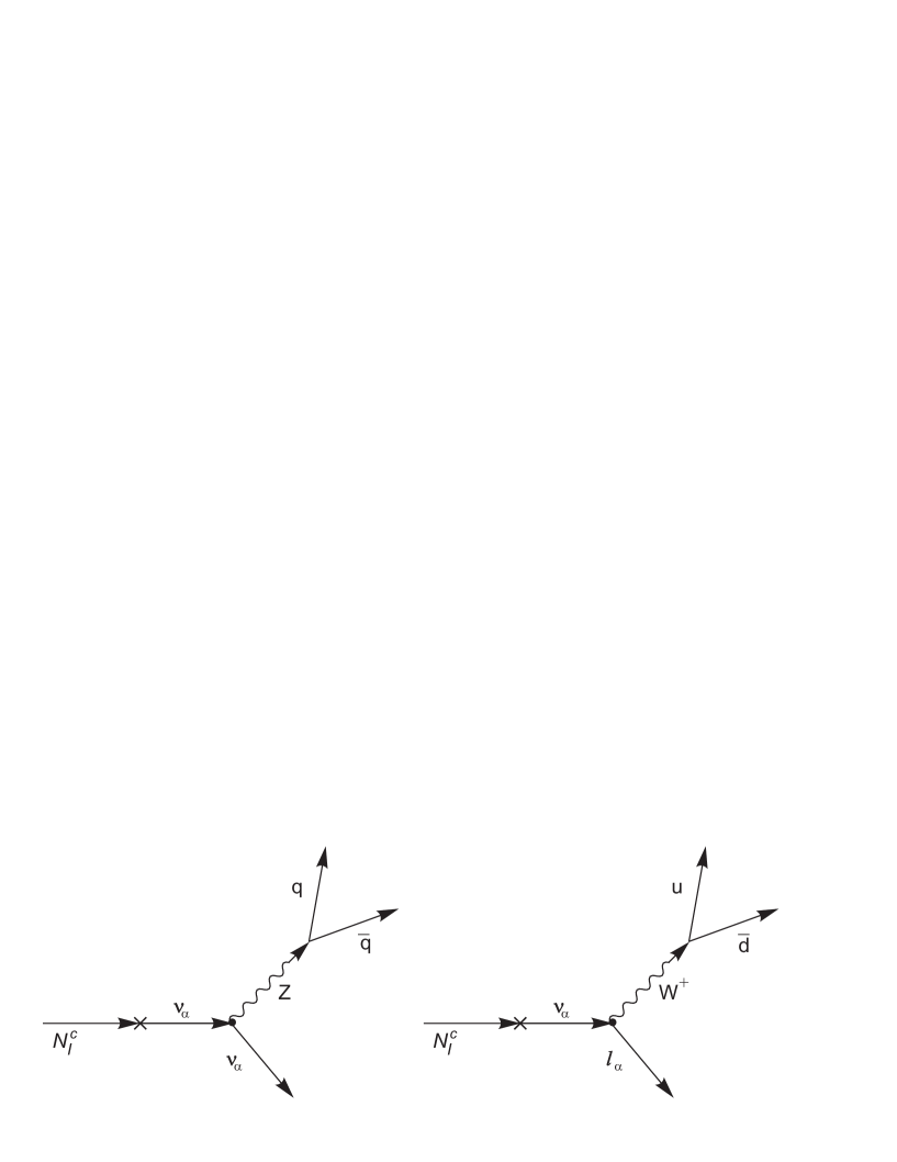
Figure 1: The decay of a sterile neutrino via $Z$-boson and $W^{+}$-boson (the cross on line of a sterile neutrino means an oscillation of a sterile to an active neutrino).

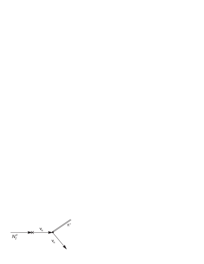
Figure 2: Effective low-energy decay of a sterile neutrino into $\pi^{0}$ meson and active neutrino.

The process of sterile neutrino decay into charged lepton and charged meson through $W^{\pm}$-boson is described by charged current interaction

$$\mathcal{L}_{C}=\frac{G_{F}}{\sqrt{2}}\left(j_{\nu}^{CC}\right)^{+}j^{\nu\,CC},$$ (36)

where $j_{\nu}^{CC}=j_{\nu}^{l\,CC}+j_{\nu}^{h\,CC}$ is charged lepton and hadron current,

$$j_{\nu}^{l\,CC}=\sum_{\alpha}{\bar{e}}_{\alpha}\gamma_{\nu}(1-\gamma^{5})\nu_{\alpha},\quad j_{\nu}^{h\,CC}=\sum_{n,m}V_{n,m}^{*}{\bar{d}}_{m}\gamma_{\nu}(1-\gamma^{5})u_{n}.$$ (37)

The indices $m,n$ run over the quark generation, $\alpha=e,\mu,\tau$ and $V$ is Kabbibo-Kobayashi-Maskawa (CKM) matrix. Similarly, the process of sterile neutrino decay into active neutrino and neutral meson through $Z$-boson is described by neutral current interaction

$$\mathcal{L}_{N}=\sqrt{2}{G_{F}}\left(j_{\nu}^{NC}\right)^{+}j^{\nu\,NC},$$ (38)

where $j_{\nu}^{NC}=j_{\nu}^{l\,NC}+j_{\nu}^{h\,NC}$ is active neutrino and hadron current,

$$j_{\nu}^{l\,NC}=\sum_{\alpha}{\bar{\nu}}_{\alpha}\gamma_{\nu}\frac{1-\gamma^{5}}{2}\nu_{\alpha},\quad j_{\nu}^{h\,NC}=\sum_{f}{\bar{f}}\gamma_{\nu}\left(t_{3}^{f}(1-\gamma^{5})-2q_{f}\sin^{2}\theta_{W}\right)f,$$ (39)

where sum over $f$ means sum over all quarks, $t^{f}_{3}$ – is the weak isospin of the quark, $q_{f}$ — is the electric charge of quark in proton charge units, notably $t^{f}_{3}=1/2,q_{f}=+2/3$ for $u,c,t$ and $t^{f}_{3}=-1/2,q_{f}=-1/3$ for $d,s,b$ quarks.

The matrix element corresponding to Feynman diagram of sterile neutrino decay (see, e.g., Fig.1,2) can be obtained from the interactive effective Lagrangian [14]. For example, effective Lagrangian of decay of $I$ sterile neutrino into the $\pi^{\pm},\pi^{0}$ final states is:

$$\mathcal{L}_{eff}^{\pi}=\frac{G_{F}}{2}M_{I}f_{\pi}\Theta_{\alpha I}\bar{\nu}_{\alpha}(1+\gamma_{5})N_{I}\pi^{0}+\\ +\left[\frac{G_{F}}{\sqrt{2}}M_{I}f_{\pi}V_{ud}\Theta_{\alpha I}\bar{e}_{\alpha}\left((1+\gamma_{5})-\frac{m_{\alpha}}{M_{I}}(1-\gamma_{5})\right)N_{I}\pi^{-}+h.c.\right],$$ (40)

where $G_{F}$ is Fermi coupling constant, $M_{I}$ is the mass of $I$-sterile neutrino, $m_{\alpha}$ is the mass of the charged lepton of $\alpha$ generation, $f_{\pi}$ is the $\pi$-meson decay constant that is defined as

$$\langle\pi^{+}|\bar{u}(1+\gamma^{5})\gamma_{\nu}d|0\rangle=-f_{\pi}\cdot(p_{\pi})_{\mu},$$ (41)

where $p_{\pi}$ is the pion 4-momentum.

The leptonic asymmetry $\epsilon$ can be defined as

$$\epsilon=\frac{\Gamma_{N\rightarrow l}-\Gamma_{N\rightarrow\bar{l}}}{\Gamma_{N\rightarrow l}+\Gamma_{N\rightarrow\bar{l}}}\,,$$ (42)

where $\Gamma_{N\rightarrow l}$ is the total decay rate of sterile neutrinos into leptons and $\Gamma_{N\rightarrow\bar{l}}$ is the total decay rate of sterile neutrinos into antileptons.

At tree level the decay rates of the sterile neutrinos into leptons and antileptons are equal. Therefore we must compute the one loop diagrams, see Fig.3. In the case of nearly degenerated sterile neutrinos the contribution from the diagrams presented at Fig.3b) can be neglected as compared with diagrams presented at Fig.3a). Indeed the propagator of the sterile neutrino in the diagrams a) type is proportional to $1/\Delta M$ in the center of mass frame. The leading order contribution to the leptonic asymmetry comes from interference between one-loop diagrams and tree-level diagrams [19]. In this case $\Gamma_{N\rightarrow l}-\Gamma_{N\rightarrow\bar{l}}\sim\Theta^{4}$ and $\Gamma_{N\rightarrow l}+\Gamma_{N\rightarrow\bar{l}}\sim\Theta^{2}$, the leptonic asymmetry is suppressed.

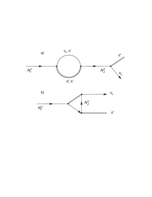
Figure 3: Example of one-loop diagrams of the decay $N_{I}\rightarrow\nu_{\alpha}\pi^{0}$.

In our case, when the mass splitting between the two heavier sterile neutrinos is very small and it is of the same order as their decay rate (we obviously will see it later), the oscillations between $N_{I}$ and $N_{J}$ are important, see Fig.4. So, the corresponding mass eigenfunctions are no longer the $N_{I}$ states, but a mixture of them, namely $\psi_{I}$ [20, 14]. It is these physical eigenstates which evolve in time with a definite frequency. The subsequent decay of these fields will produce the desired lepton asymmetry

$$\Delta=\frac{\Gamma_{\psi\rightarrow l}-\Gamma_{\psi\rightarrow\bar{l}}}{\Gamma_{\psi\rightarrow l}+\Gamma_{\psi\rightarrow\bar{l}}}\,,$$ (43)

where $\Gamma_{\psi\rightarrow l}$ and $\Gamma_{\psi\rightarrow\bar{l}}$ are the total decay rates of the sterile neutrino mass eigenfunctions $\psi_{I}$ into leptons and antileptons correspondingly. In this case the leading order contribution to the leptonic asymmetry comes from tree-level diagrams.

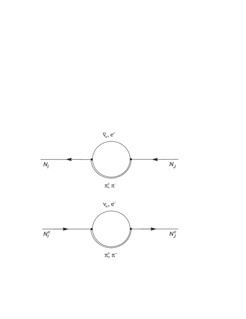
Figure 4: Contributions to the effective Hamiltonian.

In general case the correct description of the processes can be made in frame of the density matrix formalism, see, e.g., [5]. We will follow a simpler way by considering a non-hermitian Hamiltonian. The effective Hamiltonian in the basis of $\{N_{2},N_{3}\}$ is the $H=H_{0}+\Delta H$, where $H_{0}$ is the diagonal Hamiltonian of equal mass particle

$$H_{0}=\left(\begin{array}[]{cc}M&0\\ 0&M\end{array}\right).$$ (44)

The corrections to this Hamiltonian are given by the one-loop diagrams, see Fig.4:

$$\Delta H=\left(\begin{array}[]{cc}-\Delta M-\frac{i}{2}\Gamma_{2}&-\frac{i}{2}\Gamma_{23}\\ -\frac{i}{2}\Gamma_{23}&\Delta M-\frac{i}{2}\Gamma_{3}\end{array}\right).$$ (45)

The dispersive part of these diagrams can be absorbed in the mass renormalization of the fields [20] and it brings to appearance of the mass splitting $\Delta M$. The absorptive part of the diagrams will define total decay rates of the sterile neutrino $\Gamma_{I}$ and the rate of oscillation between sterile neutrinos $\Gamma_{23}$.

Total rates of $I$-sterile neutrino decays into charged mesons and leptons of $\alpha$-generation are

$$\Gamma_{I}^{\,\alpha\pi^{\pm}}=\Gamma(N_{I}\rightarrow\pi^{\pm}+l_{\alpha}^{\mp})=\\ =\frac{G_{F}^{2}f_{\pi}^{2}|V_{ud}|^{2}M^{3}}{8\pi}|\Theta_{\alpha I}|^{2}S(M,m_{\alpha},m_{\pi})\left[\left(1-\frac{m_{\alpha}^{2}}{M^{2}}\right)^{2}-\frac{m_{\pi}^{2}}{M^{2}}\left(1+\frac{m_{\alpha}^{2}}{M^{2}}\right)\right],$$ (46)

$$\Gamma_{I}^{\,\alpha K}=\Gamma(N_{I}\rightarrow K^{\pm}+l_{\alpha}^{\mp})=\\ =\frac{G_{F}^{2}f_{K}^{2}|V_{us}|^{2}M^{3}}{8\pi}|\Theta_{\alpha I}|^{2}S(M,m_{\alpha},m_{K})\left[\left(1-\frac{m_{\alpha}^{2}}{M^{2}}\right)^{2}-\frac{m_{K}^{2}}{M^{2}}\left(1+\frac{m_{\alpha}^{2}}{M^{2}}\right)\right],$$ (47)

$$\Gamma_{I}^{\,\alpha\rho^{\pm}}=\Gamma(N_{I}\rightarrow\rho^{\pm}+l^{\mp}_{\alpha})=\\ =\frac{G_{F}^{2}g_{\rho}^{2}|V_{ud}|^{2}M^{3}}{4\pi m_{\rho}^{2}}|\Theta_{\alpha I}|^{2}S(M,m_{\alpha},m_{\rho})\left[\left(1-\frac{m_{\alpha}^{2}}{M^{2}}\right)^{2}+\frac{m_{\rho}^{2}}{M^{2}}\left(1+\frac{m_{\alpha}^{2}-2m_{\rho}^{2}}{M^{2}}\right)\right],$$ (48)

where

$$S(M_{I},m_{\alpha},m)=\sqrt{\left(1-\frac{(m-m_{\alpha})^{2}}{M_{I}^{2}}\right)\left(1-\frac{(m+m_{\alpha})^{2}}{M_{I}^{2}}\right)},$$ (49)

and values of decay constants and elements of CKM matrix are given in [2]: $f_{\pi}=0.131$ GeV, $f_{K}=0.16$ GeV, $g_{\rho}=0.102$ GeV², $|V_{ud}|=0.97$, $|V_{us}|=0.23$.

Total rates of $I$-sterile neutrino decays into neutral mesons and active neutrinos are

$$\Gamma_{I}^{\,\alpha\pi^{0}}=\Gamma(N_{I}\rightarrow\pi^{0}+\nu_{\alpha})=\frac{G_{F}^{2}f_{\pi}^{2}M^{3}}{16\pi}|\Theta_{\alpha I}|^{2}\left(1-\frac{m_{\pi}^{2}}{M^{2}}\right)^{2},$$ (50)

$$\Gamma^{\,\alpha\rho^{0}}_{I}=\Gamma(N_{I}\rightarrow\rho_{0}+\nu_{\alpha})=\frac{G_{F}^{2}g_{\rho}^{2}M^{3}}{8\pi m_{\rho}^{2}}|\Theta_{\alpha I}|^{2}\left(1+2\frac{m_{\rho}^{2}}{M^{2}}\right)\left(1-\frac{m_{\rho}^{2}}{M^{2}}\right)^{2},$$ (51)

$$\Gamma_{I}^{\,\alpha\eta}=\Gamma(N_{I}\rightarrow\eta+\nu_{\alpha})=\frac{G_{F}^{2}f_{\eta}^{2}M^{3}}{16\pi}|\Theta_{\alpha I}|^{2}\left(1-\frac{m_{\eta}^{2}}{M^{2}}\right)^{2},$$ (52)

$$\Gamma_{I}^{\,\alpha\eta^{\prime}}=\Gamma(N_{I}\rightarrow\eta^{\prime}+\nu_{\alpha})=\frac{G_{F}^{2}f_{\eta^{\prime}}^{2}M^{3}}{16\pi}|\Theta_{\alpha I}|^{2}\left(1-\frac{m_{\eta^{\prime}}^{2}}{M^{2}}\right)^{2},$$ (53)

where $f_{\eta}=0.156$ GeV, $f_{\eta}^{\prime}=-0.058$ GeV [2].

As one can see the decay rates into $\rho^{\pm},\rho^{0}$ mesons are slightly different because they are vector mesons. The adduced decay rates (50) – (53) were obtained in [21, 10]. The total decay rate of sterile neutrino decay into mesons and leptons is sum of the rates over all decay channels $\Lambda$ (35) and over leptonic generation:

$$\Gamma_{I}=\sum_{\alpha,\Lambda}\Gamma_{I}^{\,\alpha\Lambda}\,\Theta(y_{\alpha\Lambda}),$$ (54)

where $y_{\Lambda}$ is the difference of the $I$ sterile neutrino mass and total mass of all final particles of the decay channel $\Lambda$; $\Theta(x)$ is the usual Heaviside function. The rate of oscillation between $I$ and $J$ sterile neutrinos ($\Gamma_{IJ}$) can be expressed through the decay rates

$$\Gamma_{IJ}=\sum_{\alpha,\Lambda}\frac{{\rm Re}(\Theta_{\alpha I}\Theta_{\alpha J}^{*})}{|\Theta_{\alpha I}|^{2}}\,\Gamma_{I}^{\,\alpha\Lambda}\,\Theta(y_{\alpha\Lambda}).$$ (55)

The eigenvalues and corresponding eigenfunctions of the non-hermitian Hamiltonian $H=H_{0}+\Delta H$ are given by

$$\omega_{2}=M-\frac{i}{4}(\Gamma_{2}+\Gamma_{3})-\frac{1}{4}c,\qquad\psi_{2}=\frac{1}{\sqrt{N}}\left(\begin{array}[]{c}B\\ 1\end{array}\right),$$ (58)

$$\omega_{3}=M-\frac{i}{4}(\Gamma_{2}+\Gamma_{3})+\frac{1}{4}c,\qquad\psi_{3}=\frac{1}{\sqrt{N}}\left(\begin{array}[]{c}1\\ -B\end{array}\right),$$ (61)

where $N$ is a normalization factor and

$$c=\sqrt{(4\Delta M-i(\Gamma_{3}-\Gamma_{2})^{2}-4(\Gamma_{23})^{2}},\quad B=(4i\Delta M+(\Gamma_{3}-\Gamma_{2})+ic)/({2\Gamma_{23}}).$$

It should be noted the sterile neutrinos are not initially in the state $\psi_{2}$ and $\psi_{3}$, but in the state $N_{2}$ and $N_{3}$. The fact is that sterile neutrino where in thermal equilibrium before they propagated freely. The equilibrium was maintained by the weak interaction between the sterile neutrinos and particles in the background. The weak interaction eigenstates are $N_{2}$ and $N_{3}$, therefore at the beginning the sterile neutrinos are in the state $N_{2}$ or $N_{3}$. In general the initial state of sterile neutrino is the superposition of $N_{2}$ and $N_{3}$ states and can be described by a density matrix:

$$\hat{\rho}_{initial}=\hat{\rho}(t=0)=\sum_{I=2,3}\alpha_{I}|N_{I}(0)\rangle\langle N_{I}(0)|,$$ (62)

where $\alpha_{2}+\alpha_{3}=1$. It was shown in [14] that leptonic asymmetry dependence on parameter $\alpha_{I}$ can be neglected. We confirmed this statement and, hereafter, we will consider the symmetric initial state $\alpha_{2}=\alpha_{3}={1}/{2}$.

The time evolution of the density matrix can be obtain in a simple way. Since

$$|\psi_{I}\rangle=U_{IJ}|N_{J}\rangle,$$ (63)

where

$$U=\frac{1}{\sqrt{N}}\left(\begin{array}[]{cc}B&1\\ 1&-B\end{array}\right),$$ (64)

the time evolution of $|N_{I}\rangle$ state is known

$$|N_{I}(t)\rangle=U^{-1}_{IK}e^{-i\omega_{K}t}|\psi_{K}(0)\rangle=U^{-1}_{IK}e^{-i\omega_{K}t}U_{KJ}|N_{J}(0)\rangle=R_{IJ}|N_{J}(0)\rangle.$$ (65)

Thus

$$\hat{\rho}(t)=\frac{1}{2}\sum_{I,J,K=2}^{3}R_{IK}(t)^{\ast}R_{IJ}(t)|N_{J}(0)\rangle\langle N_{K}(0)|=\frac{1}{2}\sum_{J,K=2}^{3}(R^{\dagger}R)_{KJ}|N_{J}(0)\rangle\langle N_{K}(0)|.$$ (66)

The average production rate of leptons is given by

$$\Gamma=\!\!\int_{0}^{\infty}\!\!\!\!\!dt\!\!\int\!\!\!d\Pi_{2}\sum_{l}Tr\left[|l\rangle\langle l|\hat{\rho}(t)\right]=\frac{1}{2}\int_{0}^{\infty}\!\!\!\!\!dt\!\!\int\!\!\!d\Pi_{2}\,Tr\left[\sum_{l,K,J}(R^{\dagger}R)_{KJ}\langle l|N_{J}(0)\rangle\langle N_{K}(0)|l\rangle\right]\!=\\ =\frac{1}{2}\int_{0}^{\infty}\!\!\!\!\!dt\!\!\int\!\!\!d\Pi_{2}\sum_{l,J,K}(R^{\dagger}R)_{KJ}A_{Jl}A_{Kl}^{\ast},$$ (67)

where sum over $l$ means sum over all leptons generations and include charged leptons and active neutrinos, $\langle l|N_{J}(0)\rangle=A_{Jl}$ is the transition amplitude of the decay of $I$ sterile neutrino into a lepton at tree level that includes all possible channels of reaction, and $d\Pi_{2}$ is the differential 2-body phase space

$$d\Pi_{2}=\frac{d^{3}q}{(2\pi)^{3}2E_{q}}\frac{d^{3}k}{(2\pi)^{3}2E_{k}}(2\pi)^{4}\delta^{4}(p-q-k),$$

where $p,q,k$ are 4-momentums of initial and final particles in decay.

Similarly the production rate of antileptons is

$$\bar{\Gamma}=\frac{1}{2}\int_{0}^{\infty}\!\!\!\!\!dt\!\!\int\!\!\!d\Pi_{2}\sum_{l,J,K}(R^{\dagger}R)_{KJ}A_{Jl}^{\ast}A_{KJ}.$$ (68)

The measure of the leptonic asymmetry is given by

$$\!\Delta\!=\!\frac{\Gamma\!-\!\bar{\Gamma}}{\Gamma\!+\!\bar{\Gamma}}\!=\!\frac{\int dt\int d\Pi_{2}Im((R^{\dagger}R)_{32})Im(A_{2l}^{\ast}A_{3l})}{\int dt\int d\Pi_{2}((R^{\dagger}R)_{22}|A_{2}l|^{2}\!+\!(R^{\dagger}R)_{33}|A_{3}l|^{2}\!+\!2Re(A_{2l}^{\ast}A_{3l})Re(R^{\dagger}R)_{23})}$$ (69)

The integration over $d\Pi_{2}$ gives [14]:

$$\Delta=\frac{\int dtIm((R^{\dagger}R)_{32})\sum_{\alpha}Im(\Theta_{\alpha 2}^{\ast}\Theta_{\alpha 3})V_{\alpha}}{\int dt\sum_{\alpha}((R^{\dagger}R)_{22}|\Theta_{\alpha 2}|^{2}+(R^{\dagger}R)_{33}|\Theta_{\alpha 3}|^{2}+2Re(\Theta_{\alpha 2}^{\ast}\Theta_{\alpha 3})Re(R^{\dagger}R)_{23})V_{\alpha}},$$ (70)

where $V_{\alpha}$ is defined via sum over all possible channels of sterile neutrino decays into leptons of generation $\alpha$

$$V_{\alpha}=\sum_{\Lambda}\frac{\Gamma_{I}^{\,\alpha\Lambda}}{|\Theta_{\alpha I}|^{2}}\,\Theta(y_{\alpha\Lambda}).$$ (71)

4 The restrictions on the parameters of the $\nu MSM$

As it was pointed in Section 1, the leptonic asymmetry of the Universe has to be constrained by condition (1) at the moment of the beginning of the DM particles production. It allows us to constrain parameters of the $\nu MSM$. To do it, we can construct the leptonic asymmetry (70) as function of only three parameters of $\nu MSM$: $M$, $\Delta M$, $\varepsilon$.

We do it in the following way. Leptonic asymmetry function (70) is maximized over phases $\delta$, $\alpha_{2}$, $\xi$ (and $\alpha_{1}$ in case of the inverted hierarchy) and is taken at central value of active neutrino mass matrix parameters, see Tab.1. This function contains dependence on ratios of the Yukawa matrix elements in mixing angle $\Theta_{\alpha I}$ (34) that can be expressed through solutions (20) with two possible choice of sign consistent with condition (22). So far as the relation for leptonic asymmetry (70) has no symmetry for interchanging and conjugating of the ratios of elements of the second and the third columns of the Yukawa matrix we have to consider two variants of the solutions. For fixed values of the mixing angles and phases we will designate allowed solution of (20) with 2 or more sign $(+)$ as solution of A type, and, vice-versa, the solution with 2 or more sign $(-)$ we will designate as solution of B type. It should be noted that our results (23), (24) for B type of solution coincide with results of [8] where the ratios of the elements were obtained in the particular case $\theta_{13}\rightarrow 0$, $\theta_{23}\rightarrow\pi/4$. We separately consider the case of $\theta_{13}=0$ and $\theta_{13}=10^{\rm o}$ also.

Thereby we construct allowed regions ($\Delta>10^{-3}$) in plane of parameters $\Delta M$ and $\varepsilon$ at fixed values of $M$.

For the case of the normal hierarchy the deference between the case of $\theta_{13}=0$ or $\theta_{13}=10^{\rm o}$ and the case of solution of A or B types is not essential, so we illustrate allowed regions with help of only one figure on Fig.5. For the case of the inverted hierarchy, the difference between the case of solution of A or B types is not essential, but the cases of $\theta_{13}=0$ and $\theta_{13}=10^{\rm o}$ are substantially different. So we illustrate allowed regions with help of two figures on Fig.6.

It should be noted that we investigated form of the allowed regions not only for the central value of $\theta_{13}$ angle, but for range given by data of [13]. We conclude that in case of the normal hierarchy the regions are almost not sensitive to value of $\theta_{13}$ in range $0<\theta_{13}<16^{\rm o}$. In case of the inverted hierarchy it is true for the regions on Fig6 b) and $\theta_{13}<18^{\rm o}$, but for $\theta_{13}=0$ the allowed regions are appreciably different.

Also we illustrate regions where maximum of $\Delta$ can be more then $2/11$ on Fig.7 (white inner figures) for the case of both hierarchies. We do it only for the mass $M=1$ GeV because this regions are at small values of $\varepsilon$ and it will not intersect with other subsequent constrains. Moreover, at some values of phases leptonic asymmetry in this region can be less then $2/11$ and so we can not exclude this region ultimately.

By way of example, we present possible values of $I$ sterile neutrino decay rate $\Gamma_{I}$ (54) and rate of oscillations between $I$ and $J$ sterile neutrinos $\Gamma_{IJ}$ (55) for $M=1$ GeV and $\theta_{13}=10^{\rm o}$ on Fig.8. As one can see the values of $\Gamma_{I}$, $\Gamma_{IJ}$ are really of the same order as $\Delta M$. It confirms previous assumption about necessity of taking into consideration oscillations between sterile neutrinos.

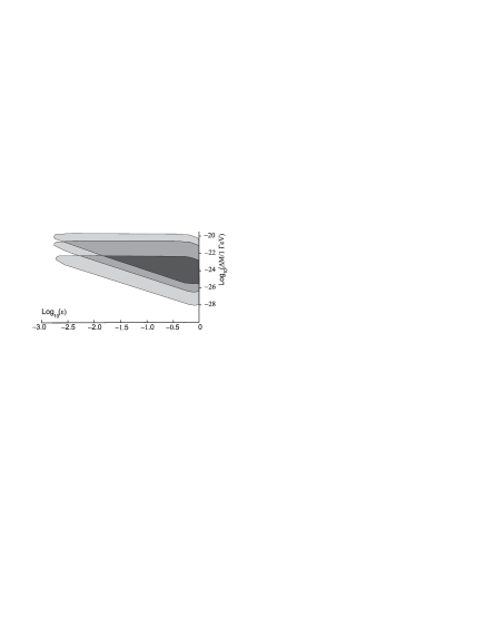
Figure 5: The grey areas are the regions of parameters where $\Delta>10^{-3}$ for the case of the normal hierarchy. The areas correspond to $M=0.3$ GeV (bottom), $M=1$ GeV (middle), $M=2$ GeV (top).

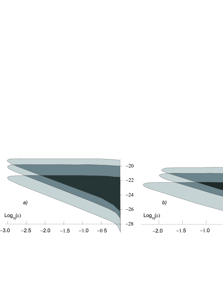
Figure 6: The grey areas are the regions of parameters where $\Delta>10^{-3}$ for the case of the inverted hierarchy. The areas correspond to $M=0.3$ GeV (bottom), $M=1$ GeV (middle), $M=2$ GeV (top). Figures a) and b) represent the case of $\theta_{13}=0^{\rm o}$ and $10^{\rm o}$ correspondingly.

In order to create a leptonic asymmetry the sterile neutrinos should be out of thermal equilibrium. That means that

$$\Gamma_{2}\lesssim H,$$ (72)

where $H$ is Hubble parameter that determines the expansion rate of the Universe. In the radiative dominated epoch Hubble parameter is given by

$$H=\frac{T^{2}}{M_{PL}^{\ast}}$$ (73)

where $M_{PL}^{\ast}=\sqrt{\frac{90}{8\pi^{3}g^{\ast}(T)}}M_{PL}$, $M_{PL}=1.22\cdot 10^{19}$ GeV is the Planck mass, $g^{\ast}(T)$ is the internal degrees of freedom [22]. At temperature $T\sim 1$ GeV we can take $g^{*}\simeq 65$.

So we get condition

$$\sqrt{M_{PL}^{*}\Gamma_{2}}\lesssim T.$$ (74)

The out-of-equilibrium condition means that sterile neutrinos should decay at a temperature smaller than their mass ($T\lesssim M$). Moreover the sterile neutrinos should decay before the creation of DM so that the leptonic asymmetry enhances the DM production. The DM is created at $T\sim 0.1$ GeV. Therefore,

$$0.1\lesssim\frac{\sqrt{M_{PL^{*}}\Gamma_{2}}}{1{\rm GeV}}\lesssim\frac{M}{1\rm GeV}.$$ (75)

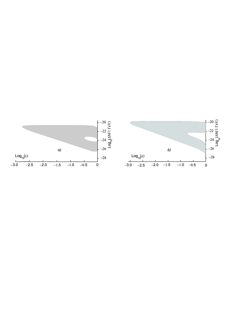
Figure 7: The grey areas represent regions of parameters where $10^{-3}<\Delta<2/11$ for $M=1$ GeV in case of normal (a) and inverted hierarchy (b).

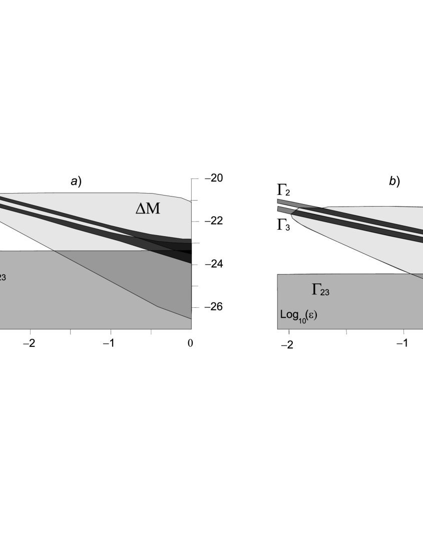
Figure 8: The values of rates $Log_{10}(\Gamma_{I}/1$GeV), $Log_{10}(\Gamma_{23}/1$GeV) and $Log_{10}(\Delta M/1$GeV) for leptonic asymmetry $\Delta>10^{-3}$ for the case of $M=1$GeV and $\theta_{13}=10^{\rm o}$ are on the ordinate axis: a) the case of normal hierarchy (A type of solution), b) the case of inverted hierarchy (B type of solution).

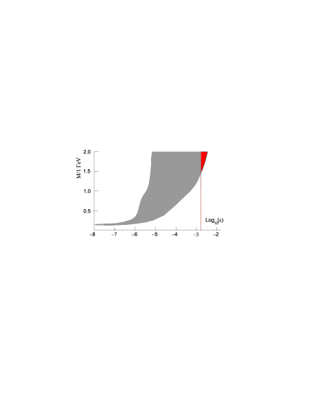
Figure 9: The case of the normal hierarchy. The points on grey and red regions satisfy constraint (75). The region on the right from vertical red line satisfies condition (1) also.

We illustrate on Fig.9 the region of values of $M$ and $\varepsilon$ where condition (75) is satisfied for the case of the normal hierarchy. At scale of parameters presented on Fig.9 the difference between the case of $\theta_{13}=0$ or $\theta_{13}=10^{\rm o}$ and between the case of solution of A or B types is small, so we present only one figure. It is not true for the case of the inverted hierarchy, see Fig.10.

It should be noted that region on Fig.9 is almost not sensitive to value of $\theta_{13}$ at range $0<\theta_{13}<16^{\rm o}$. In case of the inverted hierarchy it is true for the regions on Fig.10 b) and $\theta_{13}<18^{\rm o}$, but for the case of $\theta_{13}=0$ the regions are appreciably different.

As one can see there are regions on Fig.9 (red) and Fig.10 a) (red and blue) where conditions (1) and (75) are satisfied simultaneously. This region of parameters is suitable for DM production in the $\nu MSM$. For the case of inverted hierarchy and nonzero value of $\theta_{13}$ we have no region that is suitable for DM production. So, in $\nu$ MSM for physical nonzero value of $\theta_{13}$ and mass of sterile neutrino $m_{\pi}<M<2$ GeV DM production can be realized only in case of normal hierarchy of active neutrino mass.

The region suitable for DM production (the case of the normal hierarchy and nonzero $\theta_{13}$) can be used to obtain constraints for mass splitting of the sterile neutrino. Fixing mass of the sterile neutrino one obtains possible values of $\varepsilon$ (see Fig.9) and using Fig.5 one can obtain possible values of the mass splitting for the sterile neutrino with mass $M$. If mass of the sterile neutrino is on lower boundary of the allowed mass range ($M\simeq 1.4$ GeV) than value of $\Delta M$ is exactly known ($\Delta M\approx 5\cdot 10^{-21}$ GeV). If mass of the sterile neutrino is on upper bound of the allowed mass range ($M=2$ GeV) than $\Delta M$ can possess the values from the range $10^{-21}\lesssim\Delta M/1{\rm GeV}\lesssim 10^{-20}$.

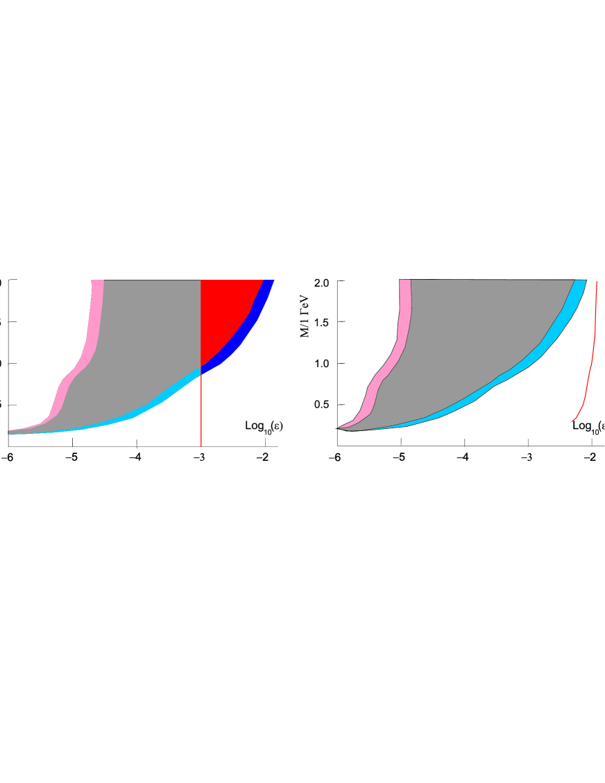
Figure 10: The case of the inverted hierarchy: a) $\theta_{13}=0$, b) $\theta_{13}=10^{\rm o}$. The pink, grey and red regions corresponds to the A type of solutions. The grey, red, sky blue and blue regions corresponds to the B type of solutions. The points on this regions satisfy constraint (75). The region on the right from red line satisfies condition (1) also.

Some existing experimental data restrict the area of parameters of $\nu MSM$. For $M<0.45$ GeV the best constraints come from the CERN PS191 experiment. For $0.45<M<2$ GeV the constraints come from the NuTeV, CHARM and BEBC experiments. The range of parameters admitted by these experimental data is summarized in [23]. These parameters are the mixing angle $(\Theta^{+}\Theta)_{22}$ (it defines the range of reactions with sterile neutrino) and the mass of the heavier sterile neutrino $M$.

To compare obtained in the present paper constraints on the $\nu MSM$ parameters (see Fig.9 and Fig.10) with constraints summarized in [23] one has to rebuild allowed regions in the space of parameters $M$ and $\theta^{2}_{\nu N_{2}}=(\Theta^{+}\Theta)_{22}$.

In general case the relation between $(\Theta^{+}\Theta)_{22}$ and $\varepsilon$ is quite difficult. Really, in accordance with (29) and(34) we have

$$(\Theta^{+}\Theta)_{22}=\frac{\nu^{2}}{2M^{2}}(V^{+}h^{+}hV)_{22}=\frac{\nu^{2}}{2M^{2}}(F_{2}^{2}+F_{3}^{2}-2|h^{+}h|_{23}\sin\chi),$$ (76)

where $\chi=arg[(h^{+}h)_{23}]$. Using (17) – (19) we get

$$F_{2}^{2}=\frac{M}{\nu^{2}\varepsilon}(m_{c}+m_{b}),\quad F_{3}=\varepsilon F_{2},\quad|h^{+}h|_{23}=\frac{M}{\nu^{2}}(m_{c}-m_{b})$$ (77)

and

$$(\Theta^{+}\Theta)_{22}=\frac{m_{c}+m_{b}}{2M\varepsilon}\left(1+\varepsilon^{2}-2\frac{m_{c}-m_{b}}{m_{c}+m_{b}}\varepsilon\sin\chi\right).$$ (78)

The problem is in parameter $\chi$ that is a complicated function of many parameters. But for our case (see Fig.9 and Fig.10, $\epsilon<0.16$) we can use approximate relation

$$(\Theta^{+}\Theta)_{22}=\frac{m_{c}+m_{b}}{2M\varepsilon}.$$ (79)

The imposition of our constraints are presented on Fig.9 and Fig.10 for nonzero value of $\theta_{13}$ and summarized constraints from [23] is presented on Fig.11. Above the line marked ”BAU”, baryogenesis is not possible: here sterile neutrinos come to thermal equilibrium above the $T_{EW}$ temperature. Below the line marked ”See-saw”, the data on neutrino masses and mixing cannot be explained using ”see-saw”  mechanism. The region noted as ”BBN” is disfavoured by the considerations of Big Bang Nucleosynthesis. The region marked ”Experiment” shows the part of the parameter space excluded by direct searches for singlet fermions. The regions market ”Cos” , ”$\Delta$”  and ”DM” were builded in this paper. The grey and blue region ”Cos”  shows the parametric space allowed by cosmological constraint (75) (grey region corresponds to A and B type of solution, blue region corresponds to B type of solution), the dashed region market ”$\Delta$”  shows the parametric space allowed by constraint (1), the red region marked ”DM”  shows the parametric space where constraints (1) and (75) are noncontradictory. The last region is preferred for DM production according to calculations of the present paper.

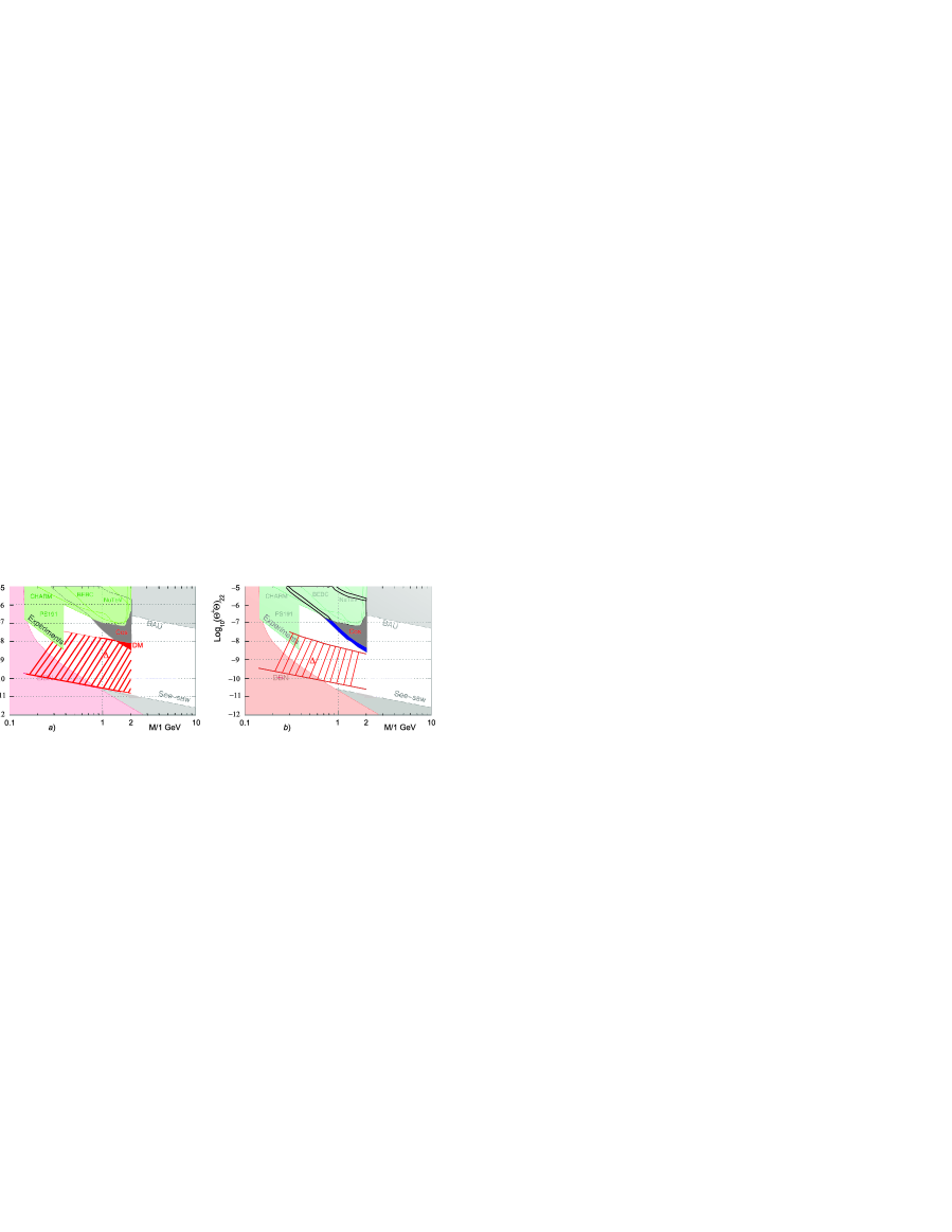
Figure 11: The imposition of our constraints and summarized constraints from [23]: a) the case of the normal hierarchy, b) the case of the inverted hierarchy.

The red region marked ”DM”  is shown on Fig.12 in the scaled-up form. The difference between the case of $\theta_{13}=0^{\rm 0}$ or $\theta_{13}=10^{\rm o}$, and between type of A or B solutions is illustrated. As one see the choice of solutions of A or B type makes greater change in the allowed region then the choice of $\theta_{13}=0^{\rm 0}$ or $\theta_{13}=10^{\rm 0}$.

5 Conclusion

In the present paper we consider the leptonic asymmetry generation at $T\ll T_{EW}$ when the masses of two heavier sterile neutrinos are between $m_{\pi}$ and 2 GeV.

We conclude that oscillations and decays of sterile neutrinos can produce a leptonic asymmetry that is large enough to enhance the DM production sufficiently to explain the observed DM in the Universe, but only for the case of the normal hierarchy of the active neutrino mass. The allowed range of parameters is narrow and it is presented on Fig.11 and Fig.12. It should be noted that allowed mass range for heavier sterile neutrino is $1.42(1.55)\lesssim M<2$ GeV for B (A) type of solutions and the mixing angle between active and sterile neutrino is $-7.91(-7.98)\lesssim{\rm Log}_{10}(\Theta^{+}\Theta)_{22}\lesssim-8.41(-8.35)$ for B (A) type of solutions. If mass of the sterile neutrino is on lower boundary of the allowed mass range than value of $\Delta M$ is exactly known ($\Delta M\approx 5\cdot 10^{-21}$ GeV). If mass of the sterile neutrino is on upper bound of the allowed mass range than $\Delta M$ can possess the values from the range $10^{-21}\lesssim\Delta M/1{\rm GeV}\lesssim 10^{-20}$. For the case of the inverted hierarchy there is no region suitable for DM production.

The big range of parameters of the $\nu MSM$ is not forbidden by the existing experimental data, see Fig.11. Combining of this range with our constraints (red region ”DM”  on Fig.11) leads to conclusion that improvement of previous experiments, as NuTeV or CHARM, of one or two order of magnitude can exclude the $\nu MSM$ with $M<2$ GeV or detect the right-handed neutrinos.

It should be noted that our constraints are quite a rough and can be used only for estimation. Really, the form of red region ”DM”  is very sensitive to cosmological constraints. Applied condition $0.1{\rm GeV}<\sqrt{M_{PL^{*}}\Gamma_{2}}<M$ is very approximate. The correct description of the processes can be made in frame of the density matrix formalism or Boltzmann equations. Our computation is not valid for $M>2$ GeV. However, the extrapolation of our result, see Fig.11, suggests that the range of admitted parameters for the case of the normal hierarchy becomes bigger for masses above 2 GeV. We expect that for masses above 2 GeV DM production can be realized for the case of inverted hierarchy too.

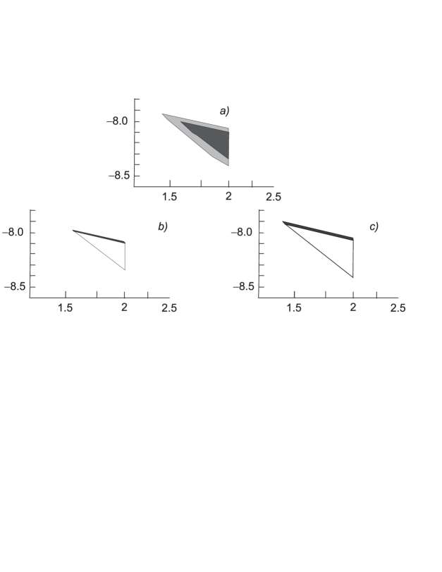
Figure 12: The red region ”DM” from Fig.10 in the scaled-up form: a) $\theta_{13}=0^{\rm 0}$ type A (dark) and type B (light); b) type A: $\theta_{13}=0^{\rm 0}$ (white) and $\theta_{13}=10^{\rm 0}$ (black); c) type B: $\theta_{13}=0^{\rm 0}$ (white) and $\theta_{13}=10^{\rm 0}$ (black). The variable M/1 GeV is along the abscissa axis and the variable ${\rm Log}_{10}(\Theta^{+}\Theta)_{22}$ is along the ordinate axis.

During computation we used two types (A or B) of solutions (20). This is due to the fact that ratios of the Yukawa matrix elements (enter into the expression for the mixing angle $\Theta_{\alpha I}$) can be expressed through solutions (20) with two possible choice of sign consistent with condition (22). It is closely related to the symmetry of (16) under replacing the elements of the second column of the Yukawa matrix by elements of the third column. This two variants are equal in rights.

The computation of the leptonic asymmetry in the applied simple model allows us to make some conclusions that, seemingly, will be correct and under more rigorous consideration. Namely, the initial state of the right-handed neutrino in form (62) are not important for lepton asymmetry generation (the final results are not sensitive to values of the constants $\alpha_{I}$). For the case of normal hierarchy the deviation of the mixing angle $\theta_{13}$ from its zero value (up to value $16^{\rm 0}$) almost does not change the region suitable for DM production. For the case of inverted hierarchy results are different for $\theta_{13}=0$ and $\theta_{13}\neq 0$. Our calculations indicates that case of $\theta_{13}=0$ leads to existing of region suitable for DM production, but at nonzero values of $\theta_{13}$ this region does not exist. Values of $\theta_{13}$ in range $\theta_{13}<18^{\rm o}$ ($\theta_{13}\neq 0$) almost does not change the region suitable for DM production.

It’s essential to note that during computations we have used functions maximized over unknown parameters of the model (phases $\delta,\xi,\alpha_{2},\alpha_{1}$). If the maximization procedure was not performed the final functions are sensitive to values of mentioned phases. So, the obtained results are very optimistic. But if the proposed on Fig.11 region of parameters ”DM” will be forbidden by experiment data it will mean that mass of heavier sterile neutrinos must be lager 2 Gev.

An essential assumption we have made is that the background effects are negligible. We do not have justify that it can be neglected in the thermal bath of the universe. For simplicity the computations were made at zero temperature. A rigorous justification of this assumptions is needed.

It should be noted that region suitable for DM production in $\nu MSM$ was recently calculated in frame of more general formalism in [24]. Certainly, results of [24] somewhat differ from our simple calculations.

References

• [1] S. Weinberg, Phys. Rev. Lett. 19, 1264 (1967); S. L. Glashow, Nucl. Phys. 22, 579 (1961); A. Salam, Proceedings of The Nobel Symposium Held 1968 At Lerum, Sweden, Stockholm 1968, 367-377.
• [2] Particle Data Group, http://pdg.lbl.gov
• [3] A. Strumia and F. Vissani, arXiv: hep-ph/0606054.
• [4] A. Boyarsky, O. Ruchayskiy, and M. Shaposhnikov, Ann. Rev. Nucl. Part. Sci. 59, 191 (2009).
• [5] T. Asaka and M. Shaposhnikov, Phys. Let. B 620, 17 (2005).
• [6] T. Asaka, S. Blanchet, and M. Shaposhnikov, Phys. Let. B 631, 151 (2005).
• [7] X.-d. Shi and G. M. Fuller, Phys. Rev. Lett. 82, 2832 (1999).
• [8] M. Shaposhnikov, JHEP 0808:008,2008.
• [9] M. Laine, M. Shaposhnikov, JCAP 0806:031,2008.
• [10] D. Gorbunov and M. Shaposhnikov, JHEP 0710:015,2007.
• [11] A. Kusenko, S. Pascoli and D. Semikoz, JHEP 0511:028,2005.
• [12] R.N. Mohapatra and A.Y. Smirnov, Ann. Rev. Nucl. Sci. 56, 569 (2006).
• [13] T2K Collaboration, Phys. Rev. Lett. 107, 041801 (2011).
• [14] T. Frossard, Leptonic Asymmetry in the $\nu MSM$ β€” 2010.
• [15] S. Bilenky and S. Petcov, Rev. Mod. Phys. 59 No. 3, Part 1 (1987).
• [16] M. Shaposhnikov, Nucl. Phys. B 763, 49 (2007).
• [17] S. Bilenky, C. Giunti, W. Grimus, Prog. Part. Nucl. Phys. 43, 1 (1999).
• [18] V. Gorkavenko, S. Vilchynskiy, Eur. Phys. J. C 70, 1091 (2010).
• [19] S. Davidson, E. Nardi and Y. Nir, Phys. Rept. 466, 105 (2008).
• [20] M. Flanz, E. Paschos, U. Sarkar and J. Weiss, Phys. Lett. B 389, 693 (1996).
• [21] L. M. Johnson, D. W. McKay and T. Bolton, Phys. Rev. D 56, 2970 (1997).
• [22] E.W. Kolb , M.S. Turner ”The early Universe”, Addison-Wesley Pub. Company, 1989.
• [23] M. Shaposhnikov, Prog. Theor. Phys. 122 , 185 (2009).
• [24] L. Canetti, M. Drewes and M. Shaposhnikov, arXiv:1204.3902, 2012.