Star Formation and AGN activity in Galaxies classified using the 1.6 $\mu$m Bump and PAH features at $z=0.4-2$.

Abstract

We have studied the star-formation and AGN activity of massive galaxies in the redshift range $z=0.4-2$, which are detected in a deep survey field using the AKARI InfraRed (IR) astronomical satellite and Subaru telescope toward the North Ecliptic Pole (NEP). The AKARI/IRC Mid-InfraRed (MIR) multiband photometry is used to trace their star-forming activities with the Polycyclic-Aromatic Hydrocarbon (PAH) emissions, which is also used to distinguish star-forming populations from AGN dominated ones and to estimate the Star Formation Rate (SFR) derived from their total emitting IR (TIR) luminosities. In combination with analyses of their stellar components, we have studied the MIR SED features of star-forming and AGN-harboring galaxies, which we summarize below: 1) The rest-frame 7.7-$\mu$m and 5-$\mu$m luminosities are good tracers of star-forming and AGN activities from their PAH and dusty tori emissions, respectively. 2) For dusty star-forming galaxies without AGN, their SFR shows a correlation that is nearly proportional to their stellar mass and their specific SFR (sSFR) per unit stellar mass increases with redshift. Extinctions estimated from their TIR luminosities are larger than those from their optical SED fittings, which may be caused by geometric variations of dust in them. 3) Even for dusty star-forming galaxies with AGN, SFRs can be derived from their TIR luminosities with subtraction of the obscured AGN contribution, which indicates that their SFRs were possibly quenched around $z\simeq 0.8$ compared with those without AGN. 4) The AGN activity from their rest-frame 5-$\mu$m luminosity suggests that their Super Massive Black Holes (SMBH) could already have grown to $\simeq 3\times 10^{8}M_{\odot}$ in most massive galaxies with $10^{11}M_{\odot}$ at $z>1.2$, and the mass relation between SMBHs and their host galaxies has already become established by $z\simeq 1-2$.

1 Introduction

A major issue in observational cosmology is to reconstruct the cosmic evolution of star formation and the detailed growth history of the present-day galaxies. Even though it is not easy to reconstruct the whole path of the stellar mass for galaxies as a function of the present-day galaxy stellar mass $M_{\ast;0}$ and the cosmic time $t$ as $M_{\ast}(M_{\ast;0},t)$, it is essential to obtain knowledge of their Star Formation Rate (SFR) as a function $SFR(M_{\ast},t)$.

Recent near-infrared (NIR) observations suggest that most of the stellar mass is contained in massive galaxies, and that this situation had already become established at $z\simeq 1$. This appears to have been followed by a rapid evolution of the stellar mass density between $z=1-3$ (Papovich et al. 2001; Dickinson et al. 2003; Fontana et al. 2003; Franx et al. 2003; Drory et al. 2004; Fontana et al. 2004; Glazebrook et al. 2004; van Dokkum et al. 2004; Labbé et al. 2005; Fontana et al. 2006; Papovich 2006; Yan et al. 2006; Webb et al. 2006; Kriek et al. 2006; Pozzetti et al. 2007; Arnouts et al. 2007; Vergani et al. 2008). These recent studies imply that most of the massive galaxies must already have formed at $z\simeq 1$, supporting the so-called downsizing scenario (Cowie et al. 1997). In this scenario, star formation shifts from higher to lower mass galaxies as a function of cosmic time $t$, although the stellar mass in massive galaxies may not directly follow the growth history of their Dark Matter Halos (DMHs) which build up hierarchically from less massive systems to more massive ones at a later time. However, several studies of massive galaxies at $z<1$ (Brown et al. 2007; Faber et al. 2007; Brown et al. 2008) report the evolution from predominantly blue to red galaxies, suggesting that the number and stellar mass of galaxies in the red-sequence may continue to grow, even after $z=1$ (Bell et al. 2004; Zucca et al. 2006), in agreement with the hierarchical merging scenario. Recently, a mass-dependent quenching of star formation has been proposed to explain these rapid increase of the number density of the massive galaxies relative to lower-mass galaxies at $z=1-2$ (Peng et al. 2010; Kajisawa 2011; Brammer et al. 2011).

The evolutionary path of the $M_{\ast}(M_{\ast;0},t)$ up to the present mass $M_{\ast;0}$ can be also reconstructed from knowledge of the $SFR(M_{\ast},t)$. Recent studies have confirmed the features for rapid SFR evolution up to $z\simeq 2$ (Brinchmann & Ellis 2000; Fontana et al. 2003; Pérez-González et al. 2005; Feulner et al. 2005a, b; Papovich 2006; Iglesias-Pramo et al. 2007; Zheng et al. 2007; Cowie & Barger 2008; Damen et al. 2009; Dunne et al. 2009; Santini et al. 2009; Pannella et al. 2009). However, we have not found a general consensus concerning the stellar mass dependence for specific SFRs: $sSFR=SFR/M_{\ast}$ (the SFR per unit stellar mass). Most studies based on UV derived SFR’s have found evidence to support an anti-correlation with stellar mass, not only local galaxies, but also the distant Universe, supporting the downsizing scenario. It is not easy, however, to accept that UV estimates are the only way to estimate the SFR that will capture all the emission originally from new born stars in a galaxy, which can be independently estimated from rest-frame luminosities in the UV, IR, Submillimeter (Submm), and radio wavelength regions by introducing appropriate calibration factors. Although the UV luminosity is used as a proxy of the SFR, its reliability often depends on the use of large, and rather uncertain corrections for dust extinction. Most of the short wavelength photons from star-forming galaxies are reprocessed through absorption and scattering with dust in their star-forming regions, and then re-emitted in the IR-Submm wavelength regions. Thus, the mid/far-IR and their submillimeter emissions become an important tracer of the total star forming activity in high-$z$ galaxies.

The total IR (TIR) luminosity $L_{IR}$ integrated across the long wavelength spectral region is a good proxy for the SFR, which is relatively independent of the dust obscuration (Kennicutt 1998). Luminous InfraRed Galaxies (LIRGs) and Ultra Luminous InfraRed Galaxies (ULIRGs) up to $z=1-2$, detected at the Mid-InfraRed (MIR) wavelength with the IR observing satellites as the ISO (Mann et al. 2002; Elbaz et al. 2002; Pozzi et al. 2004; Dennefeld et al. 2005; Taylor et al. 2005; Marcillac et al. 2006b, a), the AKARI (Takagi et al. 2007, 2010), and the Spitzer (Egami et al. 2004; Shapley et al. 2005; Caputi et al. 2006; Choi et al. 2006; Marcillac et al. 2006a, b; Papovich 2006; Papovich et al. 2006; Reddy et al. 2006; Elbaz et al. 2007; Papovich et al. 2007; Rocca-Volmerange et al. 2007; Shim et al. 2007; Teplitz et al. 2007; Brand et al. 2008; Magnelli et al. 2008; Dasyra et al. 2009; Hernán-Caballero et al. 2009; Murphy et al. 2009; Santini et al. 2009; Strazzullo et al. 2010), have shown that the SFR rapidly increases with the redshift, as they contribute $\simeq 70\%$ of the cosmic infrared luminosity density (Floc’h et al. 2005). The MIR emission from LIRGs/ULIRGs is evidence of dusty starburst or AGN surrounded by a dusty torus. Recently, the LIRGs/ULIRGs are expected to suppress star formation at $z=1-2$ with feedback activity from starbursts or AGNs. Understanding of the LIRGs/ULIRGs at $z=1-2$ can be a key to solve the cosmic history of star formation and AGN activities. The SFR for galaxies detected with the Spitzer is frequently estimated with the TIR luminosity estimated from the 24 $\mu$m flux (Daddi et al. 2004; Santini et al. 2009; Pannella et al. 2009), which is nearly proportional to their stellar mass up to $z\simeq 2$. These recent results with the Spitzer are also basically consistent with recent results from stacking analysis for their radio emissions (Dunne et al. 2009; Pannella et al. 2009) as another SFR estimation immune to dust extinctions. These two radio stacking analyses, however, show a discrepancy in their details as Dunne et al. (2009) report sSFR with a negative correlation to stellar mass while Pannella et al. (2009) report sSFR with stellar mass independence. Thus, there may be various unknown factors in the SFR estimations. The TIR luminosity $L_{IR}$ of LIRGs/ULIRGs is generally derived from the fitting of the observed Spectral Energy Distribution (SED) with synthetic templates. In the SED fitting, we could sometimes use only a few bands in the IR wavelength without longer $100-1000~{}\mu$m wavelengths, which may cause large uncertainties in the $L_{IR}$ estimation. Obscured AGNs are another notable problem in the $L_{IR}$ estimation. It means that a sample selection without significant AGN contamination is also important to obtain an accurate $SFR_{IR}$. Thus, systematically designed surveys are required to construct samples for distant star-forming galaxies.

Optical surveys have been successful in selecting numerous Lyman Break Galaxies (LBGs) as star forming galaxies beyond $z\sim 2$ (Steidel et al. 1996a, b, 1999; Lehnert & Bremer 2003; Iwata et al. 2003; Ouchi et al. 2003, 2004; Dickinson et al. 2004; Sawicki & Thompson 2006a, b) and even up to z $\simeq 6$ (Yan et al. 2004; Stanway et al. 2003; Bunker et al. 2004; Bouwens et al. 2004; Shimasaku et al. 2005). They may, however, fail to detect substantial numbers of massive galaxies at $z<3$, in which the Lyman break photometric technique does not work well with ground-based telescopes because of telluric absorption. Furthermore, even if galaxies are undergoing intensive star formation, the internal dust extinction of their UV radiation may reduce the prominence of their Lyman break features, to appear as LIRGs/ULIRGs in the local Universe. However, alternative photometric techniques can be used to select massive high-$z$ galaxies through their Balmer/4000 Å break or the 1.6 $\mu$m bump features in their Spectral Energy Distributions (SEDs), as evidence of the presence of an evolved stellar population. We will designate the former and the latter as ’Balmer’ Break Galaxies (BBGs) and as IR ’Bump’ Galaxies (IRBGs), respectively. It is known that both star-forming and passive BBGs in the redshift desert around $z=2$ can be selected with a simple and sophisticated two-color selection based on $B,z$, and $K$ band photometry (Daddi et al. 2004). This three filter optical-NIR technique was designed to detect the Balmer/4000 Å break, nearly free from the dust extinction which caused some difficulties for previous ‘red color’ techniques relying on a color diagnostic of $(R-K)_{Vega}>5-6$, corresponding to $(R-K)_{AB}>3.35-4.35$ (Elston et al. 1988; Thompson et al. 1999; Daddi et al. 2000; Firth et al. 2002; Roche et al. 2002, 2003) or for $(J-K)_{Vega}>2.3$ corresponding to $(J-K)_{AB}>1.3$ (Pozzetti et al. 2003; Franx et al. 2003). With the near-IR (NIR) observations from the Spitzer and from the AKARI, it has become possible to select IRBGs at $z>1$ with NIR colors at $>3$ $\mu$m of the 1.6 $\mu$m bump (Simpson & Eisenhardt 1999; Sawicki 2002; Berta et al. 2007). These optical-NIR observations, detecting the Balmer/4000 Å break and the 1.6 $\mu$m bump, have been also useful to trace how stellar mass is correlated with the absolute NIR luminosity.

Although optical-NIR multi-band photometry has the potential to select a sample for star-forming massive galaxies, it may not be completely free from the AGN contamination. MIR multi-band photometry tracing PAH emissions at 6.2, 7.7 and 11.3 $\mu$m and Silicate (Si) absorption at 10 $\mu$m (rest-frame) from dusty star-forming regions, can be used to discriminate between the star-forming activity in LIRGs/ULIRGs and that of AGN dominated galaxies. Thus, systematic multi-wavelength observations that include observations at $>2~{}\mu$m are important for studies the star-forming activity of massive high-$z$ galaxies, and in looking back at the evolution of their SFRs. In order to connect the history of stellar mass growth in massive galaxies traced in optical-NIR wavelength with ground based telescopes and that of star formation traced in MIR wavelength observed outside of the atmosphere, we undertook multi-wavelength surveys of deep and wide areas with $\simeq 0.38$ and $\simeq 5.8$ deg², respectively, in a field close to the North Ecliptic Pole (NEP), which were extensively observed at the IR wavelength with the first Japanese infrared astronomical satellite AKARI.

In this paper, we attempt to reconstruct the cosmic history of dusty massive galaxies up to $z\simeq 2$, selected estimated from optical-IR images in the NEP survey field. We report on: 1) photometric redshift $z_{phot}$, stellar mass $M_{\ast}$, and $SFR_{UV;cor}$, which are estimated with their optical-NIR SED fittings, 2) the distinction between dusty starburst and AGN dominated galaxies using the MIR SED feature, 3) TIR luminosities of starburst dominated galaxies with the subtraction of the obscured AGN contribution, from which we can derive $SFR_{IR+UV}$ complementary to the $SFR_{UV:cor}$, and 4) IR luminosities of the dusty tori of AGN dominated galaxies, which show evolutionary trends in the connection between AGN and star forming activities.

In section 2, we summarize the data we used; in section 3, we present the photometry for $z^{\prime}$-band detected galaxies in our multi-wavelength dataset; in section 5, we also report AKARI/IRC detected IRBGs classified using the redshifted 1.6-$\mu$m IR bump in the NIR bands, which are divided into three redshifted subgroups; in section 6, we present AKARI/IRC MIR detected galaxies which correspond to LIRGs/ULIRGs and classify them into dusty starbursts and AGN from their MIR SEDs with/without PAH features in the MIR bands; in section 7, we derive the TIR luminosities for the MIR detected galaxies; in section 8, we estimate their star formation rates and extinctions; in section 9, we reconstruct their intrinsic stellar populations with extinction correction; in section 10 we also study the AGN activities in the MIR detected galaxies; in section 11, we discuss some expectations for on-going and future observations; finally in section 12, we summarize the conclusions of our study.

In this paper we adopt $H_{0}=70$ km s^-1 Mpc^-1, $\Omega_{m}=0.3$, $\Omega_{\Lambda}=0.7$ throughout. All magnitudes are represented in the AB system (e.g. Oke 1974).

2 The data set

We have used mainly the data sets obtained in the AKARI Deep imaging survey with all of the available bands of the Infra Red Camera (IRC) on the AKARI (Onaka et al. 2007) near the North Ecliptic Pole (NEP). We define the $N2,~{}N3,~{}N4,~{}S7,~{}S9W,~{}S11,~{}L15,~{}L18W$, and $L24$ bands as having central wavelengths at 2, 3, 4, 7, 9, 11, 15, 18, and 24 $\mu$m respectively. These are reported in this paper as the IR photometric AB magnitude of an object observed in the various IRC bands. Details of the data reduction of the NEP Deep and Wide surveys have been presented by Wada et al. (2008) and Lee et al. (2007) (see also Hwang et al. (2007) and Ko et al. 2012), respectively. We have used the same IRC scientific data for the AKARI NEP Deep field as described in detail by Wada et al. (2008), which include mosaicing them together and making pointing and distortion corrections, as well as correction to mitigate detector artifacts.

The AKARI NEP Deep survey area has been covered by observations in the near-UV $u^{\ast}$ band with the CFHT/MegaCam(M-Cam) (Boulade et al. 2003); the optical $B,V,R,i^{\prime}$, and $z^{\prime}$ bands with the Subaru/Suprime-Cam (S-Cam) (Miyazaki et al. 2002); and in the NIR $J$ and $K_{s}$ bands with the KPNO(2.1m)/Flamingos(FLMG) (Elston et al. 2006). Details of the Subaru/S-Cam, CFHT/M-Cam, and KPNO/FLMG data reduction can be found in Imai et al. (2007), Takagi et al. (2012), and Ishigaki et al. (2012). In this study, we have selected $\simeq 56000$ galaxies with $z^{\prime}<26.4$ and S/N$>3$. For these sources, we estimate their multi-wavelength photometric characteristics, adding ground-based near-UV, optical, and NIR imaging data to the AKARI/IRC data as described in the following Section. For simplification, we use $u,i,z$, and $K$ as $u^{\ast},i^{\prime},z^{\prime}$ and $K_{s}$, respectively for representing colors derived from the respective filters.

3 Photometry

Table 1: Summary of photometric parameters.

Band	FWHM	FWHM	Ap.D.
	(pixel)	(arcsec)	(arcsec)
$u^{\ast}$	4.9	0.90	3.0
$B,V,R,i^{\prime},z^{\prime}$	5.2	1.00	2.0
$J$(SE)	2.7	1.60	3.0
$J$(NE)	3.1	1.90	3.0
$J$(SW)	3.0	1.80	3.0
$J$(NW)	3.5	2.10	4.0
$K_{s}$(SE)	2.7	1.60	3.0
$K_{s}$(NE)	3.0	1.80	3.0
$K_{s}$(SW)	3.7	2.20	4.0
$K_{s}$(NW)	3.2	1.90	4.0
N2,N3,N4	3.1	4.50	8.0
S7,S9W,S11	2.4	5.60	10.0
L15,L18W,L24	2.8	6.70	10.0
The S-Cam FoV of $34^{\prime}\times 27^{\prime}$ is covered with 4 FLMN FoV, in which each covers the $25^{\prime}\times 30^{\prime}$ area.

Table 2: Summary of limiting magnitudes and photometric corrections.

Band	$m_{lim.}$	$\Delta m_{a.c.}$	$\Delta m_{g.e.}$	$\Delta m_{s.o.}$
	[AB]	[AB]	[AB]	[AB]
$u^{\ast}$	26.31	-0.06	-0.20	+0.20
$B$	28.25	-0.24	-0.18	+0.00
$V$	27.57	-0.24	-0.13	-0.02
$R$	27.41	-0.24	-0.11	-0.11
$i^{\prime}$	27.14	-0.24	-0.09	-0.07
$z^{\prime}$	26.40	-0.24	-0,06	-0.13
$J$(SE)	22.28	-0.22	-0.04	+0.02
$J$(NE)	22.22	-0.27	-0.04	+0.02
$J$(SW)	22.23	-0.28	-0.04	+0.02
$J$(NW)	21.83	-0.20	-0.04	+0.02
$K_{s}$(SE)	21.66	-0.22	-0.02	-0.09
$K_{s}$(NE)	21.58	-0.22	-0.02	-0.09
$K_{s}$(SW)	21.34	-0.22	-0.02	-0.09
$K_{s}$(NW)	21.20	-0.19	-0.02	-0.09
N2	21.89	-0.24	-0.01	-0.08
N3	22.24	-0.24	-0.01	+0.12
N4	22.49	-0.24	-0.01	+0.13
S7	20.29	-0.20
S9W	20.00	-0.22
S11	19.82	-0.24
L15	19.60	-0.27
L18W	19.60	-0.26
L24	18.60	-0.27
$m_{lim.}$ is the limiting magnitude. $\Delta m_{a.c.}$ is the aperture correction in magnitude. $\Delta m_{g.e.}$ is the magnitude correction for galactic extinction in the field. $\Delta m_{s.o.}$ is the magnitude correction for systematic offset with the SED calibration for the stellar objects.

3.1 Optical and NIR photometry for ground-based data

Object detection and photometry were made using SExtractor 2.3.2 (Bertin & Arnouts 1996). The $z^{\prime}$ S-Cam image was used to detect optical objects, defined as a source with a 5 pixel connection above the 2 $\sigma$ noise level. We derived the Full Width Half Maximum (FWHM) of the Point Spread Function (PSF) from the photometric images of stellar objects as point sources (see their selection scheme in subsection 3.4), which are summarized in table 1. In the process to make a catalogue, the reason why the $z^{\prime}$-band was chosen as the detection band is the following: 1) the FWHM of the PSF $1"$ in the $z^{\prime}$ image with the S-Cam is good enough to prevent the confusion, 2) the $z^{\prime}$ photometry is one of the essential bands in the star-galaxy selection with the $BzK$ color as shown in subsection 3.4, 3) most of the galaxies of interest as detected by the AKARI; N3 Red Galaxies (N3Rs) and MIR bright N3Rs (MbN3Rs), and optical-NIR selected galaxies as BBGs are clearly identified in the $z^{\prime}$ image. See the details about the N3Rs, the MbN3Rs, and BBGs in subsections  5.1 and  6.1, and in appendix A), respectively. The catalogue of detected objects to $z^{\prime}<26.4$ with a 2^′′ diameter aperture was generated over the whole 23^′ $\times$ 32^′ area of the S-Cam $z^{\prime}$ image.

After selecting $\sim$ 56000 $z^{\prime}$ sources in the area observed with the FLMG, from the $\sim$ 66000 sources detected in the S-Cam $z^{\prime}$ images, we performed aperture photometry in the near-UV $u^{\ast}$, optical $B,V,R,i^{\prime},z^{\prime}$, and NIR $J,K_{s}$ images, fixed at the positions of the $z^{\prime}$-detected sources. The photometry on the $B,V,R,i^{\prime}$, and $z^{\prime}$ images was performed with a small 2^′′ diameter aperture with the SExtractor. The photometry on the $u^{\ast}$ and the $J$ and $K_{s}$ images was performed with larger 3^′′ and 4^′′ diameter apertures with the photo of the IRAF task since these image qualities in off-center regions are not good due to the aberrations compared with those of the S-Cam. The larger aperture photometry reduces the uncertainties in the photometry and the alignment errors in the World Coordinate System (WCS) from these aberrations. The errors of the ground-based optical and NIR photometry come mainly from the sky background and its fluctuation. We have estimated them from a Monte Carlo simulation with the same method as that of Ishigaki et al. (2012), in which we measured the counts in randomly distributed apertures and fit the negative part of the count histogram with a Gaussian profile. Thus, the 3$\sigma$ limiting magnitudes $m_{\lim}$ were derived from the background estimation, as summarized in table 2.

The final integrated magnitudes for all filters were obtained after applying an aperture correction $\Delta m_{a.c.}$ based on empirical PSFs, which are constructed from the photometry for stars in each image band. All of the optical and NIR magnitudes were further corrected for a galactic extinction of $E(B-V)=0.041$, based on observations of the survey area taken from Schlegel et al. (1998) and using the empirical selective extinction function of Cardelli et al. (1989).

3.2 Infrared photometry for AKARI/IRC images

As shown above, we have produced a multiband merged catalogue from the ground-based telescope images for the $z^{\prime}$-detected objects in the field. As shown in table 2, the depth of $N2$ images obtained with the AKARI/IRC is comparable to that of $K_{s}$ images with the KPNO/FLMG, although the images of all other bands at longer wavelengths are shallower than those of $z^{\prime}$. In fact, from 5819 sources extracted with the SExtractor in the N3 band with a 5 pixel connection above the 2 $\sigma$ noise level, $92\%$ of them can be identified as 5332 counterparts of $z^{\prime}$-detected sources without confusion. Thus, we have performed the photometry for all of the AKARI/IRC bands on the $z^{\prime}$-detected sources.

The IRC photometry on the $z^{\prime}$-detected sources was performed with 8^′′ and 10^′′ diameter apertures for NIR ($N2,N3$, and $N4$) and MIR ($S7,S9W,S11,L15,L18W$, and $L24$) bands, respectively, with the IRAF task photo.

The final integrated magnitudes in the IRC photometry were obtained after applying an aperture correction based on the growth curves with empirical PSFs, constructed from photometry of stars in each band image, which is basically similar to the scheme descirbed in Takagi et al. (2012). The aperture corrections for the IRC are summarized in table 2, along with those of the ground-based near-UV, optical, and NIR magnitudes.

In order to reduce the source confusion due to the fact that the IRC PSFs are notably worse than those in the ground-based observed images, we have performed IRC photometry with several different apertures in each IRC band, and compared these magnitudes, excluding objects with a large magnitude difference from the IRC counterparts in the $z^{\prime}$-detected catalogue. In the photometry in $N2,N3$, and $N4$ bands, we have optimized the constraint for the IRC/NIR counterparts as $N3(6")-N3(8")<0.51$ between $6^{\prime\prime}$ and $8^{\prime\prime}$ diameter photometry in the $N3$ band, adding another constraint of $Ks-N2<1.0$ at 2 $\mu$m.

For MIR sources detected with SN3 at least in one MIR band, there were many more sources with confusion compared with the NIR sources. We could select $\sim$ 800 MIR bright N3 Red galaxies (MbN3Rs) and $\sim$ 900 MIR marginally-detected N3 Red galaxies (MmN3Rs) as shown in section 6. However, we have taken confirmed samples of $\sim 600$ MbN3Rs and $\sim 600$ MmN3Rs after excluding NIR counterparts of the MIR sources having pairs within 6$"$, in order to correctly select the candidates of LIRGs at $z>0.4$ as discussed in section 6. Roughly two thirds of these MbN3Rs and MmN3Rs were also identified as sources listed in another MIR source catalogue reported by Takagi et al. (2012), which are almost the same after taking the difference in their detection limits into consideration, as the former was selected with $SN>3$ at least in one MIR band while the latter was with $SN>5$. Concerning these NIR and MIR detected galaxies, we could confirm with our eyes that it can work to mostly exclude confusion from neighborhood sources within a circleregion corresponding to the IRC PSF radius around each $z^{\prime}$ source.

3.3 Photometric check and systematic offsets

In order to further check the photometric zero points, we have performed SED fitting with $u^{\ast}BVRi^{\prime}z^{\prime}JK_{s}$ and AKARI $N2,N3,$ and $N4$ photometric data for the stellar objects. It is well known that galactic stars can be clearly selected using a two-color criterion (Daddi et al. 2004; Kong et al. 2006; Lane et al. 2007; Quadri et al. 2007; Blanc et al. 2008):

$$BzK_{\ast}\equiv(z-K)_{\rm AB}-0.3(B-z)_{\rm AB}<-0.3\;,$$ (1)

where we have taken $-0.3$ as a parameter in the right side, which defines a line separating stars and galaxies that is slightly larger than Daddi’s original value of $-0.5$, to reduce the contamination of stars in our galaxy sample. We have used the $BzK$ color criterion to select the photometric calibrators as stellar objects with additional criteria for the magnitudes $z^{\prime}>19$ and stellarity parameter CLASS_STAR $>0.95$ in SExtractor (see also subsection 3.4). We have also excluded IRC/NIR confused image sources by visual examination.

We have adopted SED templates from the stellar library of Bruzual-Persson-Gunn-Stryker (BPGS) Atlas, based on Gunn & Stryker (1983), which is similar to the Pickles (1998) stellar spectra, and Lejeune et al. (1997). In order to include the $N4$ magnitudes in our fitting of SEDs to the stellar objects with the BPGS Atlas, we have extended the library SEDs beyond wavelengths of $\lambda>2.5~{}\mu$m with a Rayleigh-Jeans law. The best fit is sought by means of $\chi^{2}$ minimization, among all templates in the stellar library after varying their normalization. We have estimated the offsets in each of the bands, which are seen as systematic discrepancies between the original observed magnitudes and the best-fitted library magnitudes. These systematic offsets are also summarized in table 2. Since the derived offsets are less than $0.2$, basically we can confirm the accuracy of the photometric zero points in all the bands. In the comparison between the spectroscopic and photometric redshifts, the result for the systematic offset is slightly better than that without this. Thus, we use the offset.

3.4 Star-galaxy separation

As discussed in subsection 3.3, the colors estimated with the BPGS star atlas overlap with the observed stellar sequence appearing in the $BzK$ color region (see figure 44 in the appendix). Thus, we can also use the $BzK$ criterion of equation (1) as a robust method for star-galaxy separation. For sources detected with $SN>3$, up to $K_{s}=20$, we have excluded objects satisfying the following conditions; 1) equation (1) and 2) stellarity parameter CLASS_STAR$>0.95$ in SExtractor. In order to separate stars and galaxies for all of the $z^{\prime}$-detected objects up to an optical limiting magnitude $z^{\prime}=26$ that are fainter than the above $K_{s}$ detected sources, we performed SED fittings for them with not only the BC03 models (Bruzual & Charlot 2003) for galaxies but also the BPGS star atlas for stellar objects, including those corrected with Allen’s Milky Way extinction curves. We extracted objects as stellar objects, which were fitted better by the latter than the former, from catalogue of $z^{\prime}$-detected galaxies (see also subsection 4.1). These stellar objects appear in the sequences of the BPGS star atlas in BBG color-color diagrams (see not only figure 44, but also figures 45, and 46 in appendix A).

4 Photometric redshifts

Figure 1: Comparison between spectroscopic and photometric redshifts for $z^{\prime}$-detected galaxies with spectroscopic observations. Filled diamonds and open circles represent objects with and without broad line emissions in their spectra, respectively. Dashed lines represent a deviation with $\Delta z/(1+z_{spec})=0.1$.

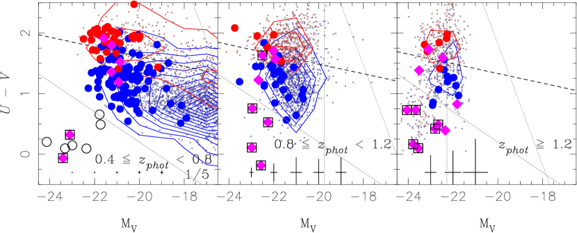
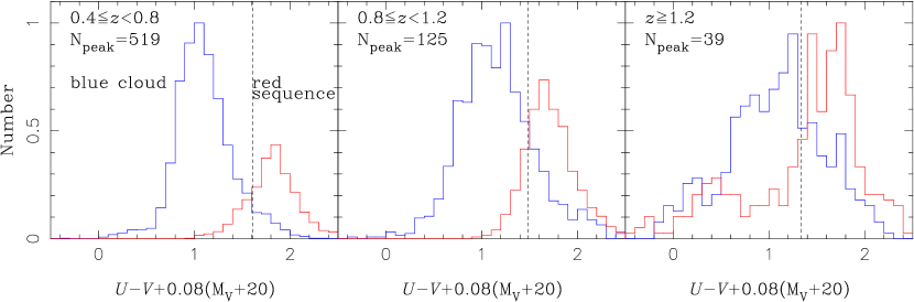
Figure 2: Rest-frame color $U-V$ for the spectroscopic sample and $z^{\prime}$-detected galaxies. Top: Rest-frame Color Magnitude Diagram (CMD) of absolute $V$-band magnitude vs. $U-V$ color. Objects in redshift ranges of $0.4\leq z<0.8$, $0.8\leq z<1.2$, and $1.2\leq z$ are represented from the left to the right. Large symbols represent the spectroscopic sample. Red and blue symbols represent lower and higher SFR populations with sSFR $<0.1$ Gyr^-1  and sSFR $>0.1$ Gyr^-1  derived from the SED fitting, respectively. Magenta diamonds represent BL AGNs, in which diamonds in squares represent outlier BL AGNs with $\Delta z/(1+z_{spec})>0.2$ in the redshift comparison. Small gray dots represent the remainder in the $z^{\prime}$-detected galaxies. Red and blue contours represent the distribution of lower and higher SFR population in the $z^{\prime}$-detected galaxies with sSFR $<0.1$ Gyr^-1  and sSFR $>0.1$ Gyr^-1, respectively. Dashed lines represent Bell’s color boundary between star-forming and passive populations. Plain black crosses around $U-V\simeq-0.2$ represent typical errors of estimated colors and mass. The vertical solid and steep slope dense dotted lines represent the limiting absolute $V$ and $U$-band magnitudes at the mean redshift, respectively. Open circles represent a population categorized as type 1 QSOs at $z=0.2-0.7$ in the catalogue of the SDSS/SWIRE sample by Hatziminaoglou et al. (2005). Bottom: Color distributions of the $z^{\prime}$-detected galaxies. The color is scaled as $(U-V)+0.08(M_{V}+20)$. Red and blue lines represent lower and higher SFR populations with sSFR $<0.1$ Gyr^-1  and sSFR$>0.1$ Gyr^-1  derived from the SED fitting, respectively.

4.1 Photometric and spectroscopic redshifts

For all of the $z^{\prime}$-detected galaxies remaining after the star-galaxy separation procedure as described in subsection 3.4, we simultaneously obtained the photometric redshift $z_{phot}$ and the absolute magnitude $M_{H;opt}$ corresponding to the stellar mass $M_{\ast}$ (see also appendix G), by applying a photometric redshift code hyperz (Bolzonella et al. 2000). This is based on comparison of the observed ground-based $u^{\ast}BV$$Ri^{\prime}z^{\prime}$$JK_{s}$ photometry with a grid of stellar population synthesis models produced from Bruzual & Charlot (2003). From this BC03 model we prepared SED templates of a total of nine star-forming history models with exponential decaying star formation (SF) as $SFR(t)\propto\exp(-t/\tau)$, with time scales for the star formation activity of $\tau=0.1,0.3,1,2,3,5,15,\mbox{and}~{}30$ Gyr, and we varied the age $t$ from 0 to 20 Gyr, and included the Constant Star Formation (CSF) model. All of the models are for solar metallicity. With the variations of $E(B-V)=0,0.1,0.2,0.3,0.4,0.5,$ and $0.6$, we additionally applied Allen’s Milky Way, Seaton’s Milky Way, LMC, SMC, and Calzetti’s extinction curves, to obtain the extinction $A_{V}$. In selecting the best fitting one from five extinction curves for each object, firstly we determine a median photometric redshift $z_{m}$ in five of them related to these extinction models, and secondly we have used one model with reduced $\chi^{2}$ minimization as the photometric redshift should be within 0.2$(1+z_{m})$ around the median $z_{m}$. We adopted a Salpeter IMF from 0.1 to 100 M_⊙ throughout this work.

In the AKARI NEP Deep field, we also obtained spectra with the KeckII/DEIMOS, the Subaru/FOCAS, and the MMT/Hectospec for 420, 57, and 62 objects, which were selected from objects with $R<24,<24$, and $<22$ mag, respectively. The KeckII/DEIMOS and the Subaru/FOCAS observations partially covered the NEP Deep field while the MMT/Hectospec observations covered the NEP Deep field by two, 1 deg² multi-object configurations. More details on the MMT/Hectospec observations can be found in Ko et al. (2012). They are mostly detected as IR sources with the AKARI (Takagi et al. 2010). We have obtained 292 spectra for the $z^{\prime}$-detected galaxies, in which we can determine secure redshifts for 230 objects are detected with more than two lines or clearly with [OII] line. They include 27 galaxies harboring AGN with Broad Line (BL) emissions, which are spectroscopically classified as BL AGNs. Figure 1 shows the comparison between the spectroscopic and the photometric redshifts of the 230 objects and their redshift discrepancy $\Delta z=z_{phot}-z_{spec}$. The median accuracies of $\langle\Delta z\rangle/(1+z_{spec})$ are 0.041 and 0.038 for the spectroscopic samples without and with excluding the BL AGNs, respectively. In the spectroscopic sample, there are the 22 and 52 outliers with $\Delta z/(1+z_{spec})>0.2$ and $>0.1$, in which 11 and 12 out of these outliers are BL AGNs, respectively. Thus, the photometric redshifts are consistent with their spectroscopic ones not only for the samples except BL AGNs but also for even half of the BL AGNs. The outlier BL AGNs except one are confirmed as an Extremely Blue Object (EBO) in the rest-frame Color-Magnitude Diagrams (CMDs), which are selected with a criterion:

$$(U-V)<-0.25(M_{V}+22.0)+0.7\;,$$ (2)

as shown in figure 2. If EBOs are type 1 AGNs, this trend is reasonable since SED models of the AGNs were not included in SED fittings for the photometric redshift estimations.

The AKARI MIR colors can alternatively extract candidates associated with dusty AGN activities, in which we spectroscopically observed 14 agn-MbN3Rs and 2 s/a-MbN3Rs (see the details about them in subsection 6.1). We could confirm that 8 out of 14 agn-MbN3Rs and 2 out of 2 s/a-MbN3Rs show the discrepancy with $\Delta z/(1+z_{spec})>0.1$, respectively. All of these outliers are also identified as BL AGNs, in which 7 out of 8 the agn-MbN3Rs and 2 out of 2 the s/a-MBN3Rs are classified as the EBOs, respectively. As long as their redshifts are correctly obtained with spectroscopy, the overlap of the EBOs with the agn-MbN3Rs suggests that the dust emission detected as the agn-MbN3Rs should coexist with optically blue emission classified as the EBOs in all of them. This supports not only the above expectations that AGNs are harbored in the EBOs and the agn-MbN3Rs but also a picture of a dusty torus surrounding AGN which can explain the variation of their SEDs as frequently proposed in the AGN unified theory.

We also checked the redshift discrepancy $\Delta z$ in various populations subclassified not only with the spectroscopy, but also with NIR and MIR photometry as N3Rs and MbN3Rs, which are summarized in appendix C. Even though most of the spectroscopic samples are mainly selected from dusty populations with heavy extinction as MbN3Rs detected in the AKARI MIR photometry, their median accuracies of $\langle\Delta z\rangle/(1+z_{spec})$ are less than 0.05 for any subclassified populations of N3Rs and MbN3Rs except agn-MbN3Rs. Their photometric redshifts can be estimated well from the SED fitting with their major stellar emission of the host galaxies, in which the extinctions might not be a serious matter. Thus, the estimated photometric redshifts even for most of the galaxies can be used to reconstruct approximately their actual redshifts within $\Delta z/(1+z_{spec})<0.05$.

4.2 Reconstructions of rest-frame magnitudes and colors

From the derived photometric redshifts $z_{phot}$ with the optical-NIR SED fittings, we can also estimate rest-frame magnitudes and colors of the $z^{\prime}$-detected galaxies. For an object at a redshift $z$, a magnitude $m_{\lambda_{0}}(z)$ at a rest-frame wavelength $\lambda_{0}$ is approximately interpolated from the observed magnitudes as

$$m_{\lambda_{0}}(z) = \frac{\left[\lambda_{r}-\lambda(z)\right]m_{b}+\left[\lambda(z)-\lambda_{b}\right]m_{r}}{\lambda_{r}-\lambda_{b}}\;,$$ (3)

$$\lambda(z) = \lambda_{0}(1+z)\;,$$ (4)

where $m_{r}$ and $\lambda_{r}$ ($m_{b}$ and $\lambda_{b}$) are the observed magnitudes and central wavelengths of the band neighboring the red-side (blue-side) of the observing wavelength $\lambda(z)$. By using the rest-frame magnitudes derived with $z_{phot}$, CMDs for the $z^{\prime}$-detected galaxies can be obtained. The CMD fundamentally is almost the same as the color-mass diagram, which is a powerful tool for studying galaxy evolution since it shows the bimodal galaxy distribution as early types concentrate on a tight red sequence while late types distribute in a blue dispersed cloud. This has been studied not only in the local Universe with the SDSS (Blanton et al. 2003) but also in the distant Universe with surveys for $z<1$ (Bell et al. 2004; Faber et al. 2007; Borch et al. 2006) and for $z>1$ (Pannella et al. 2009; Brammer et al. 2009).

Figure 2 shows a CMD of the absolute $V$-band magnitude $M_{V}$ and $U-V$ color. We display rest-frame $V$-detected galaxies on the CMD, and excluded objects with less photometric accuracy of $SN<2$ in the rest-frame $V$ band. The rest-frame $U-V$ color straddles the Balmer/4000 Å break and is also essential to introduce classifications for their stellar populations in IRBGs, MbN3Rs, MmN3Rs, and BBGs as discussed in the following sections and the appendix. This interpolation scheme, applied for the $z^{\prime}$-detected galaxies with $z=z_{phot}$, can be used to derive their $M_{V}$ and rest-frame $U-V$ colors. In figure 2, we can see that the distribution of galaxies is bimodal up to $z\simeq 1$ as previously shown (Bell et al. 2004; Faber et al. 2007; Borch et al. 2006). In figure 2, we can see that the red sequence and the blue cloud are separated with a criterion:

$$(U-V)=1.15-0.31z-0.08(M_{V}-5\log h+20)\;,$$ (5)

which is introduced for the definition of red sequence galaxies by Bell et al. (2004) and represented as dashed lines on the CMDs in figure 2. Thus, our catalogue of $z^{\prime}$-detected galaxies with photometric redshifts is basically the same as those of other blank sky surveys.

5 Classification with IR bump

From the sample of $z^{\prime}$-detected galaxies including the Balmer Break Galaxies (BBGs; see the details in appendix A), we extracted IR classified subpopulations with the AKARI/IRC photometry. The NIR IRC photometry can select IR bump Galaxies (IRBGs) which have a bump around 1.6 $\mu$m with the AKARI (Takagi et al. 2007) and the Spitzer (Berta et al. 2008). Both the IRBGs and the BBGs are characterized mainly by the emission from the stellar components. In this section, we will present three redshifted populations selected by criteria of the IR bump at 1.6 $\mu$m combining the Balmer break. In fact, the selection with the 1.6 $\mu$m can reduce the contamination from the low-z interlopers in the IRBGs at $z>0.4$, which is also useful to classify MIR-bright populations. We also try to select AGN candidates as outliers with NIR colors redder than normal IRBGs.

5.1 AKARI NIR color-color diagram and 1.6 $\mu$m bump

Table 3: The Parameters for IRBG Selections

IRBGs	$f_{\scriptsize{N23}}$	$\min_{\scriptsize{N34}}$	$\max_{\scriptsize{N34}}$	$z_{\mbox{\scriptsize{min}}}$	$z_{\mbox{\scriptsize{max}}}$
N3R	$-0.3$	–	–	$0.4$	–
N23	$-0.3$	–	$-0.5$	$0.4$	$0.8$
N34	$-0.3$	$-0.5$	$-0.1$	$0.8$	$1.3$
N4R	$-0.3$	$-0.1$	–	$1.3$	$-$

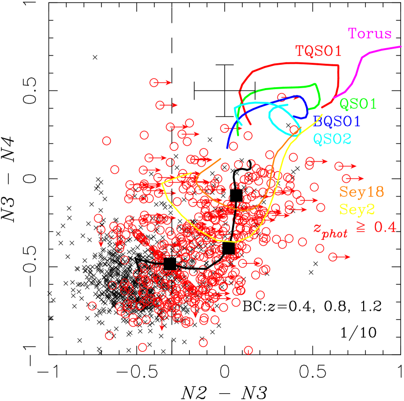
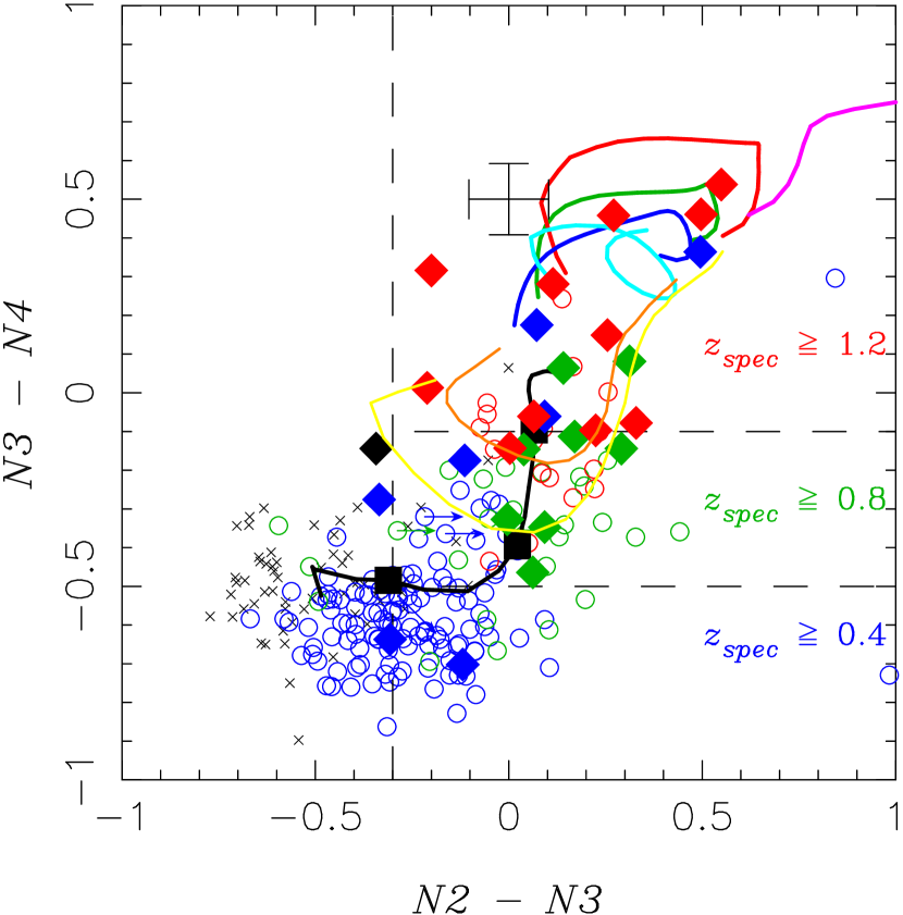
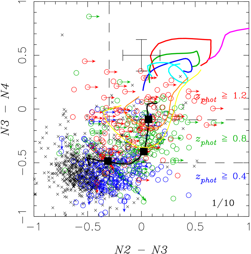
Figure 3: Two-color diagram of $N2-N3$ vs. $N3-N4$ in the field. Symbols of cross bar at $(N2-N3,N3-N4)=(0.1,0.5)$ represent typical errors of the color. Black line is superimposed as a redshifted track of a BC03 model galaxy with $\tau=1$Gyr and age$=1$Gyr, on which the squares are related to the redshifts of $z=0.4,0.8,$ and $1.2$ from lower-left to upper-right. Other superimposed green, red, blue, cyan, and magenta lines are tracks of QSO1, TQSO1, BQSO1, QSO2, and dusty torus IR templates, respectively. Redshift from $z=0$ to $z=2$ corresponds to the upper-right to the lower-left along each line. Top: For objects detected in the $N2,N3,$ and $N4$ bands. Arrows represent objects which are fainter than the threshold limit in the $N2$ or $N4$ band. Red open circles and black crosses represent the objects at $z_{phot}\geqq 0.4$ and $z_{phot}<0.4)$, respectively. Bottom-Left: For the spectroscopic samples. Blue, green, and red symbols represent the objects at $0.4\leq z_{spec}<0.8$, $0.8\leq z_{spec}<1.2$, and $z_{spec}\geqq 1.2$, respectively. Diamonds represent BL AGNs. Bottom-Right: The same as on the left for the photometric samples.

A bump centered at 1.6 $\mu$m in the rest-frame is a major SED feature of galaxies except for the youngest ones for ages $<10$ Myr, in which stellar components are dominated by type M stars. The 1.6 $\mu$m IR bump is produced by the combination of the spectral peak in black-body radiation from low-mass cool stars as M stars and a minimum in the opacity of H^- ion present in their stellar atmospheres with molecular absorptions (John 1988). Universally appearing in most galaxies, the IR bump is one of the most useful SED features in their photometric measurements (Simpson & Eisenhardt 1999; Sawicki 2002).

The AKARI NIR photometry in $N2N3N4$ bands can trace the IR bump at $z=0.4-2$. We have shown the redshift tracks of the BC model galaxies with $\tau=1$Gyr and age$=1$Gyr on a two-color diagram of $N2-N3$ vs. $N3-N4$ in figures 3, where the solid squares on the tracks represent the redshifts at $z=0.4,0.8$, and 1.2 from the bottom-left to the top-right. The tracks are mostly parallel to the $N2-N3$ axis up to $z\simeq 0.8$, bending upward around $z\simeq 0.8$, and are vertical along the $N3-N4$ axis at $z\simeq 0.8-1.2$. This trend can be understood as the excess of redshifted IR bump is on the $N2$ side in the $N3$ band at $z\simeq 0.4-0.8$, the $N4$ side in the $N3$ band at $z\simeq 0.8-1.2$, and in the $N4$ band at $z>1.2$. The redshift is the dominating factor in determining the AKARI NIR color tracks of galaxies without AGNs while the galaxy type is less effective.

First, we extract $N3$-detected ones as $N3$ Red galaxies (N3Rs) possibly at $z>0.4$ from the $z^{\prime}$-detected galaxies with a criterion:

$$N2-N3>f_{\scriptsize{N23}}\;.$$ (6)

Second, we can also subclassify the N3Rs into N23, N34, and N4 bumpers, which are defined as IRBGs of their IR bump detected with the $N2$ and $N3$ bands, the $N3$ and $N4$ bands, and the $N4$ band in three redshift ranges of $z\simeq 0.4-0.8$, $z\simeq 0.8-1.2$, and $z>1.2$, respectively. The color criteria are represented as

$$N2-N3>f_{\scriptsize{N23}}\;\cap\;\;\mbox{min}_{\scriptsize{N34}}\leq N3-N4<\mbox{max}_{\scriptsize{N34}}\;,$$ (7)

where the parameters of $f_{\scriptsize{N23}},\min_{\scriptsize{N34}}$, and $\max_{\scriptsize{N34}}$ are given in table 3.

The bottom-left of figure 3 represents a two-color diagram for the spectroscopic sample in the field, in which most of the galaxies at $z_{spec}\simeq 0.4-0.8,0.8-1.2$, and $>1.2$ appear as N23, N34, and N4 bumpers, respectively. The bottom-right of figure 3 also represents another two-color diagram for the photometric sample in the field, in which the NIR color of galaxies at $z_{phot}\simeq 0.4-0.8,0.8-1.2$, and $>1.2$ distribute around the regions of N23, N34, and N4 bumpers, respectively.

When a galaxy harbors an AGN, however, IR emission from the dusty torus around the AGN affect the NIR colors. We have also superimposed tracks of redshifted QSO SED templates in the SWIRE library ; three types of optically-selected type 1 QSOs (QSO1, TQSO1, and BQSO1) and two models of type 2 QSOs (QSO2 and Torus). All of them show dominant emissions from the dusty torus at IR wavelength $\lambda>1~{}\mu$m. Thus, the NIR color criterion from equation (6) can be still effective for selecting not only galaxies at $z>0.4$ but also AGN candidates. Furthermore, all the QSO tracks are overlapping with the region of the N4 bumpers. In fact, most of the BL AGNs, selected with the spectroscopy, appear around the region of N4 bumpers. Thus, the N3Rs with $N3-N4>-0.1$ may include not only the N4 bumpers of IRBGs but also these AGN candidates, which will be also confirmed with the MIR classified AGNs in section 6. We will designate the N3Rs with $N3-N4>-0.1$ as N4 Red galaxies (N4Rs).

5.2 N3Rs subclassified with Balmer break

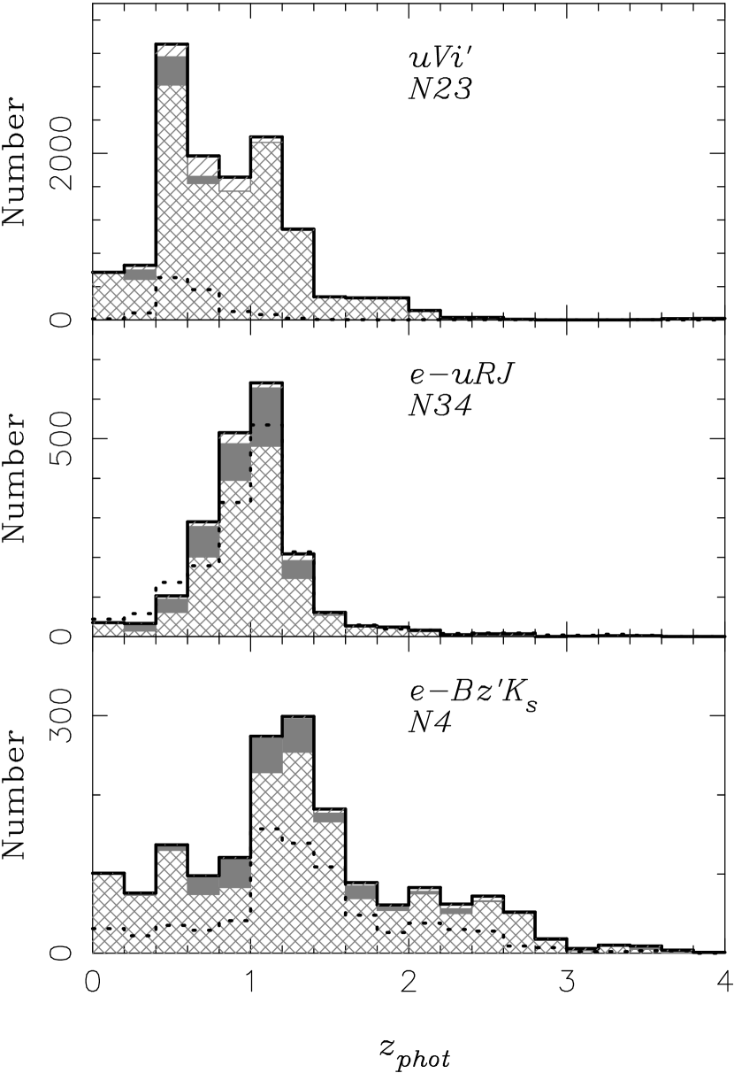
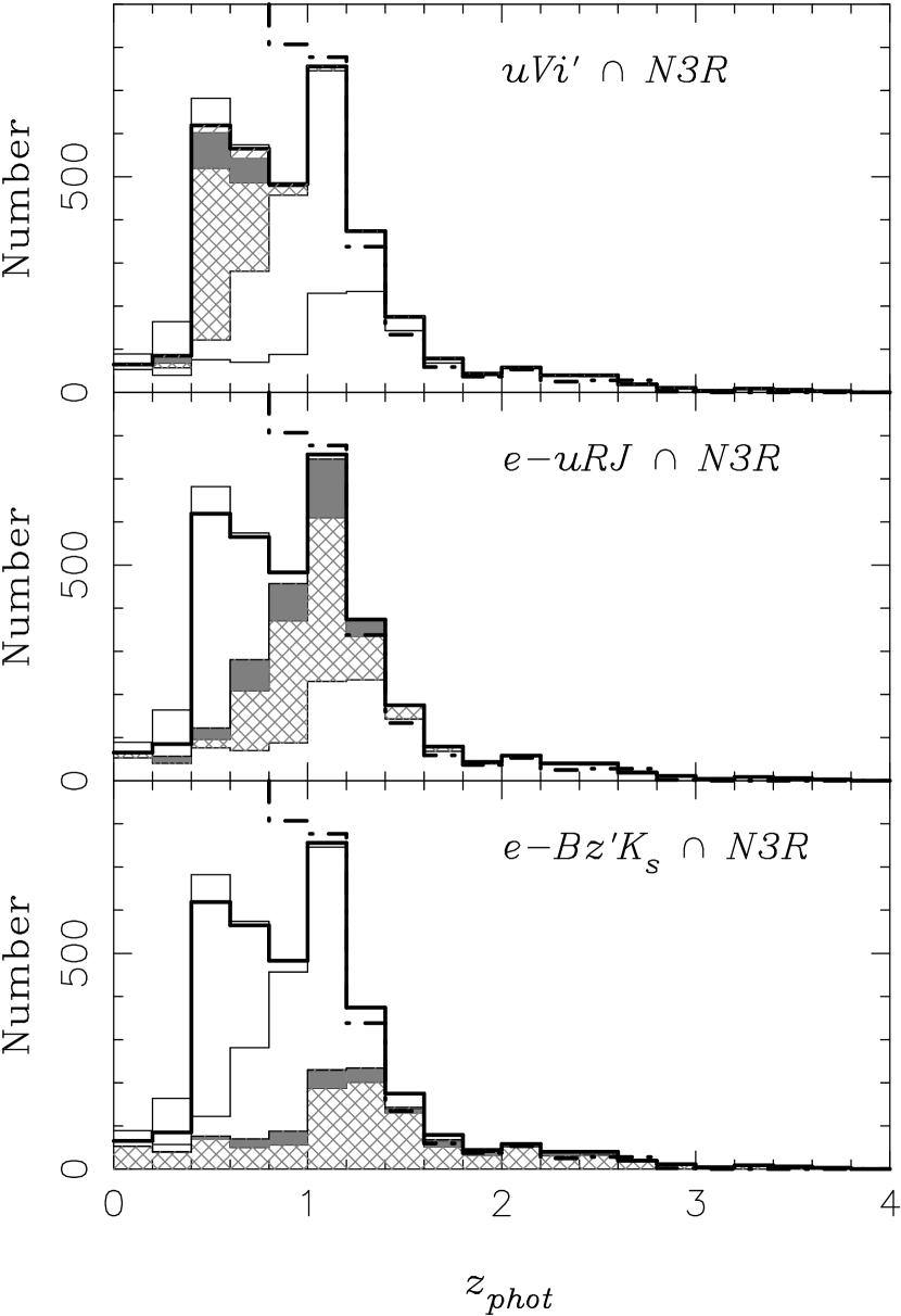
Figure 4: The photometric redshift distributions for exclusively classified BBGs; e-BzKs, exclusively classified e-uRJs from the remainings after exclusion of the e-BzKs, and exclusively classified uVis from the remainings after exclusion of both the e-BzKs and the exclusively classified e-uRJs, from bottom to top. Shaded, single-hatched, and cross-hatched area represent p-, qp-, and s-BBGs. Left: For exclusively classified BBGs and IRBGs. Dotted lines represent N23 bumpers, N34 bumpers, and N4Rs, from top to bottom. Right: For N3 Red BBGs. Dashed, thin solid and thick solid lines represent the rest-frame $V$-detected galaxies, the N3Rs, all the N3 Red BBGs, respectively.

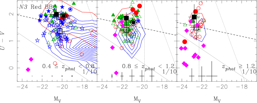
Figure 5: The same as figure 2 for N3 Red BBGs. The plots for $0.4<z<0.8$, $0.8<z<1.2$, and $1.2<z$ from left to right. In general, colored open, solid, and circled symbols represent objects classified as s-, p-, and qp-BBGs, respectively. Basically, red circles, green triangles, and blue stars represent objects selected with the two-color criteria as e-BzKs, e-uRJs, and uVis, respectively. Black-large open, solid, and circled symbols represent mean values for the s-, p-, and qp-BBGs, respectively. Crosses on their black symbols represent their standard deviations. Only a part of samples are plotted to reduce crowding in the diagram, whose fractions are presented as numbers in the right-bottom region of all figures.

As shown in figure 3, both spectroscopic and photometric redshifts of the N3Rs are almost consistent with the NIR color criterion $N2-N3>-0.3$ of the IR bump at $z>0.4$. As mentioned in subsection 4.1, the photometric redshifts were derived from only the ground-based data without the AKARI NIR data, which means that the selection with the IR bump is independent of the photometric redshifts. Thus, the color criterion with $N2-N3>-0.3$ is useful in order to exclude low redshift interlopers at $z<0.4$ in the IRBGs as long as they are detected in the $N2$ (or $K$) and $N3$ bands as discussed in subsection 5.1. Furthermore, adding the AKARI/NIR photometry to the ground-based optical-NIR photometry can salvage the BBGs in the IRBGs as shown in appendix A.3. These are the merits in using the AKARI/NIR photometry with the ground-based photometry.

On the other hand, even though the IR bump criteria of N23 and N34 bumpers, and N4Rs correspond to three redshift intervals as shown in figure 3, they cannot be robust for the redshift subclassification since the N4Rs possibly include AGNs as discussed in subsection 6.2. In redshift subclassifications, optical color criteria with the Balmer break are more reliable than those of the $N3-N4$ colors with the IR bump. As described in appendix A, we have generalized the color criteria of BzKs at $1.4<z<2.5$ with $BzK$ filter set (Daddi et al. 2004) to select BBGs at $0.8<z<1.8$ and $0.4<z<0.8$ by using $uRJ$ and $uVi$ filter sets, called as uRJs and uVis, respectively. Furthermore, we have selected extended BBGs as e-BzKs and e-uRJs with the $N3$ band photometry which is the deepest one in the IRC bands (see appendix A.3). However, these e-BzKs, e-uRJs, and uVis overlap each other. Thus, we introduced an exclusive subclassification of BBGs as first picked with the $BzK$ criteria, second applied the $uRJ$ criteria for those remaining after exclusion of the BzKs, and finally applied the $uVi$ criteria for those remaining after exclusion of the uRJs and the BzKs. As shown on the left in figure 4, the redshift distributions of the exclusively classified BBGs except the uVis are similar to those of IRBGs as the uRJs and the BzKs correspond to the N34 bumpers and the N4Rs, respectively. Most counterparts of the MIR bright populations at $z>0.4$, detected with the AKARI MIR photometry in the field, are identified as the N3Rs. Thus, hereafter, we will take a subclassification of the N3Rs into the star-forming (s-), passively evolving (p-), and quasi passively evolving (qp-) BBGs with the exclusively subclassification. We will name these BBGs exclusively subclassified from the N3Rs as N3 Red BBGs (N3RBBGs); N3RBzKs, N3RuRJs, and N3RuVis. The redshift distributions of N3 Red BBGs are also shown on the right in figure 4. Figure 5 shows the CMD of $M_{V}$ and $U-V$ for these N3 Red BBGs. We can see that the subclassification of the s-, p-, and qp-N3RBBGs is consistent with that using Bell’s color boundary in figure 5.

Since the $N3$ band photometry is the deepest one in the IRC bands, as discussed in appendix A.3, the N3 Red BBGs salvaged with the $N3$ photometry are almost the same selected population as the rest-frame $V$-detected galaxies at $z>0.4$. It can be confirmed as both of them show a similar redshift distribution as shown in figure 4. The rest-frame $V$-detected galaxies are a kind of referenced sample as frequently plotted with the referenced contours on the CMDs in figures 2 and  5 (see also figures  48 and  50 in the appendix). Thus, the N3 Red BBGs are suitable in the study for their stellar populations by using the CMD even in MIR bright populations as seen in section 6.

6 Classifications with MIR SEDs

The MIR multi-band photometry with the IRC has identified MIR-bright populations in the N3Rs as detected with more than an SN3 in MIR bands and classfied into starbursts or AGNs with two MIR color diagrams, which are called as MbN3Rs. The IRC MIR photometry can detect Poly-Aromatic Hydrocarbon (PAH) emissions from dusty star-forming regions for a subgroup in the IRC detected MbN3Rs. The subgroup with the PAH features can be classified with the MIR colors as starbursts, which are overlapped with the PAH luminous galaxies in some companion papers (Takagi et al. 2007, 2010). Another subgroup of the MbN3Rs without any PAH features or with weak ones is possibly AGN dominant. Some of them may overlap with Power-Law Galaxies (PLGs) and IR Excess Galaxies (IREGs), which are already classified with the Spitzer as AGN-dominant populations. The former has MIR SEDs well fitted by a power law (Lacy et al. 2004; Stern et al. 2005; Alonso-Herrero et al. 2006; Donley et al. 2007). The latter shows the large infrared-to-UV/optical flux ratio (Daddi et al. 2007; Dey et al. 2008; Fiore et al. 2008; Polletta et al. 2008), in which some may be identified as sources with heavily obscured optical emissions. The MbN3Rs and their relatives at $z>0.4$ detected in the field have typically TIR luminosities with $>10^{11}$L_⊙, which correspond to those of LIRGs/ULIRGs as shown in appendix D. In this section, thus, we will mainly study the MbN3Rs and their relatives by analyzing the MIR and NIR SEDs to reveal star forming and AGN activities of LIRGs/ULIRGs at $z>0.4$ in the following sections.

6.1 Starburst and AGN in MIR bright N3Rs

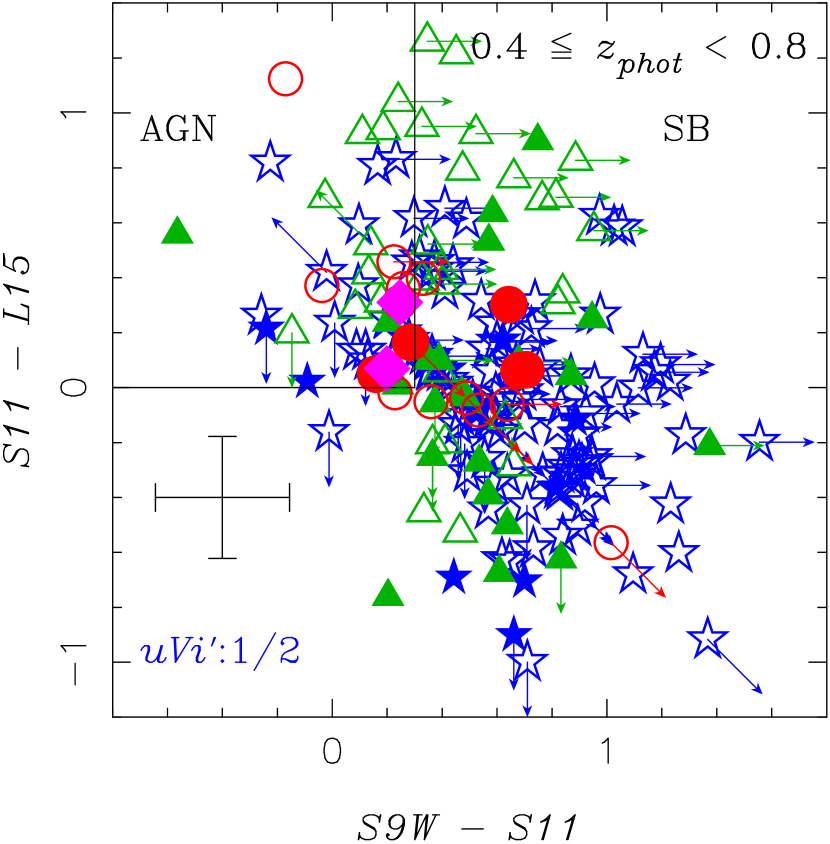
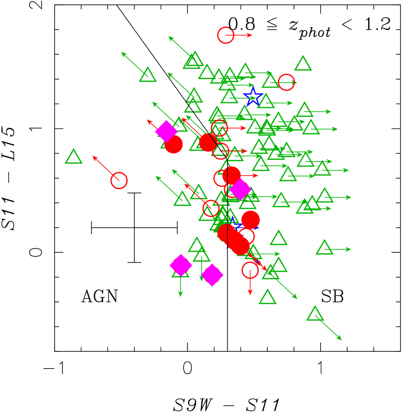
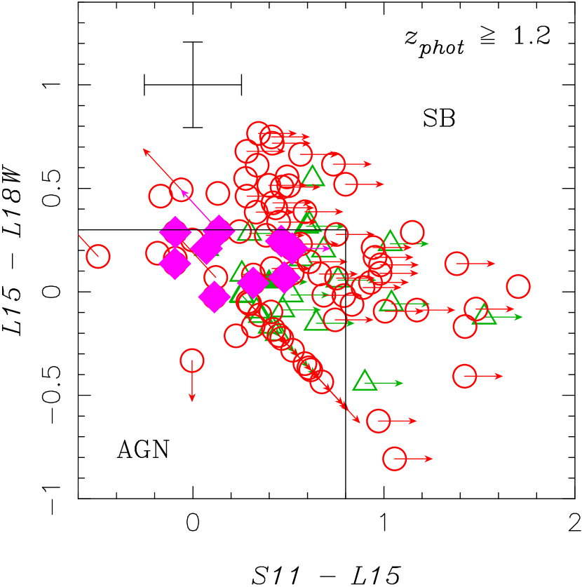
Figure 6: MIR color-color diagrams for the MbN3Rs, which are also subclassified into s/p/qp-BBG/N3Rs and BL AGNs. Blue stars, green triangles, and red circles represent s(p)-uVis, s(p)-(uRJs+uRN3s+BRN3s), and s(p)-(BzKs+uzN3s+BzN3s), respectively. Diamonds represent the spectroscopic BL AGNs. Top-Left: The $S9W-S11$ vs. $S11-L15$ diagram for the observed MbN3Rs at $0.4\leq z<0.8$. Top-Right: The same as the Top-Left, for the MbN3Rs at $0.8\leq z<1.2$ with the tracks in $0.8\leq z<1.4$. Bottom: The $S11-L15$ vs. $L15-L18W$ diagram for the MbN3Rs at $0.8\leq z<1.2$ with the tracks in $1.0<z<2.8$.

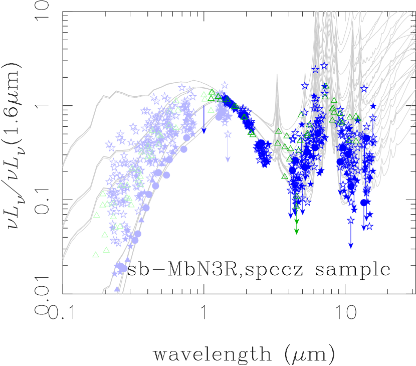
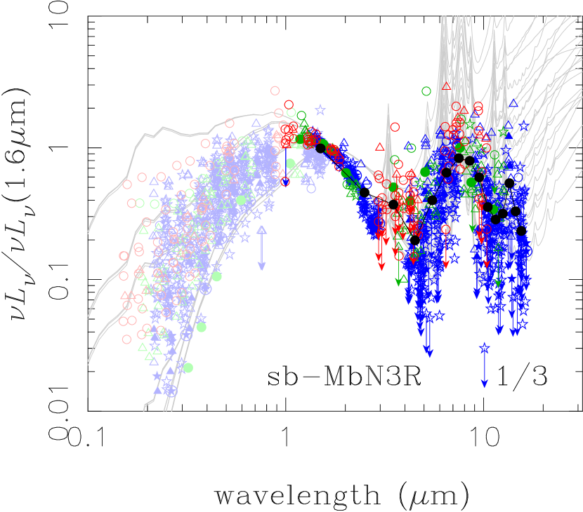
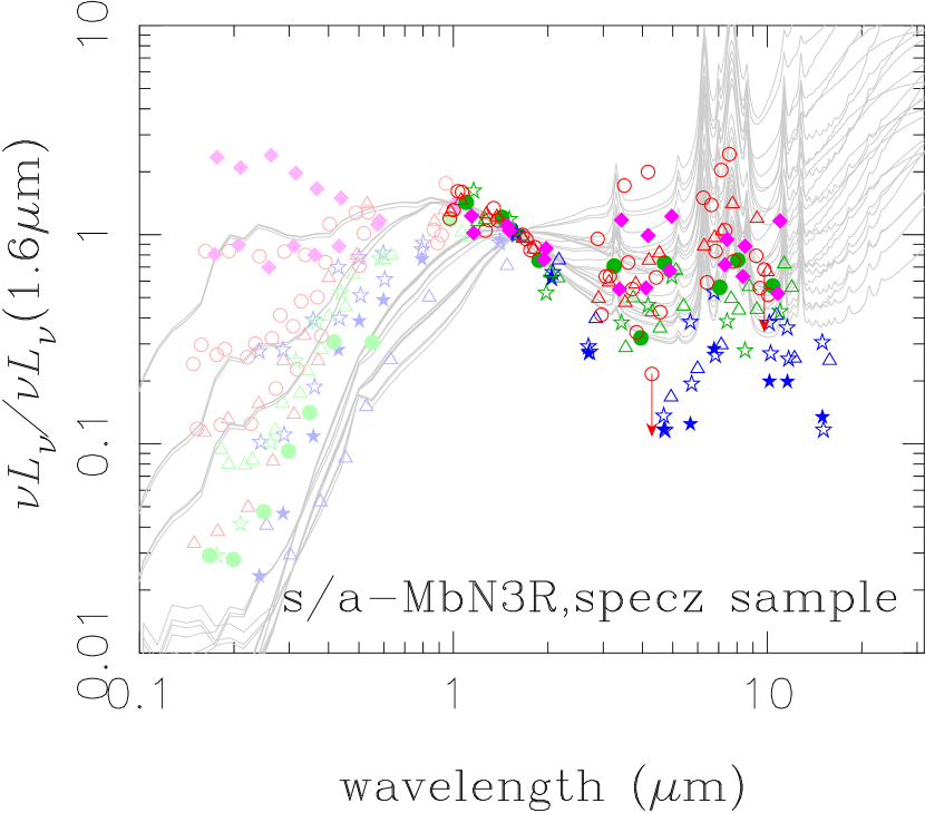
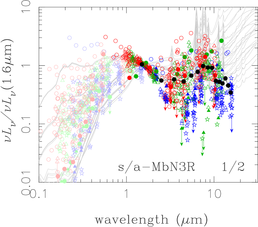
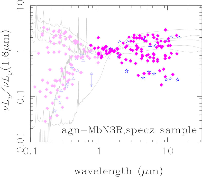
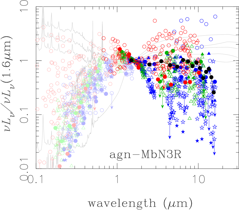
Figure 7: Rest-frame SED normalized at 1.6 $\mu$m for the MbN3Rs. Symbols are the same as figure 6 except for their colors. Blue, green, and red symbols represent the redshifts of $0.4\leq z<0.8$, $0.8\leq z<1.2$, and $z\geq 1.2$, respectively. Dark and faint symbols represent AKARI IRC photometric data and ground-based photometric data, respectively. The averaged observed MIR SEDs are represented with solid lines in the figures on the right. Top-Left: For the sb-MbN3Rs in the spectroscopic sample. Superimposed lines represent dusty starburst SED templates of the S&K models used in the MIR SED fitting. Top-Right: The same as on the left for the sb-MbN3Rs in the photometric sample. Middle-Left: The same as the Top-Left for the s/a-MbN3Rs in the spectroscopic sample. Superimposed lines represent SEDs composed of the S&K models and the dusty torus model in the SWIRE SED library with the ratio of 0.3 to 0.7 at 5$~{}\mu$m. Middle-Right: The same as on the left for the s/a MbN3Rs in the photometric sample. Bottom-Left: The same as the Top-Left for the agn-MbN3Rs in the spectroscopic sample. Superimposed lines represent the SWIRE SED templates of dusty torus, QSO2, BQSO1, TQSO1, and QSO1 from top to below at the long wavelength. Bottom-Right: The same as on the left for the agn-MbN3Rs in the photometric sample.

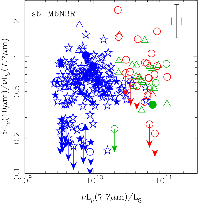
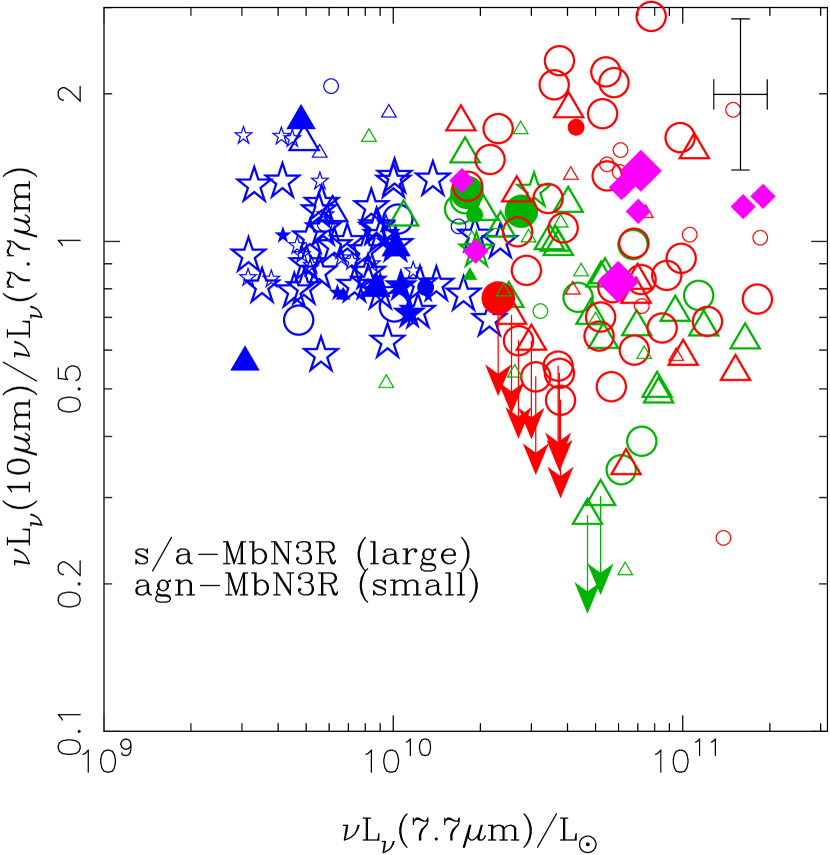
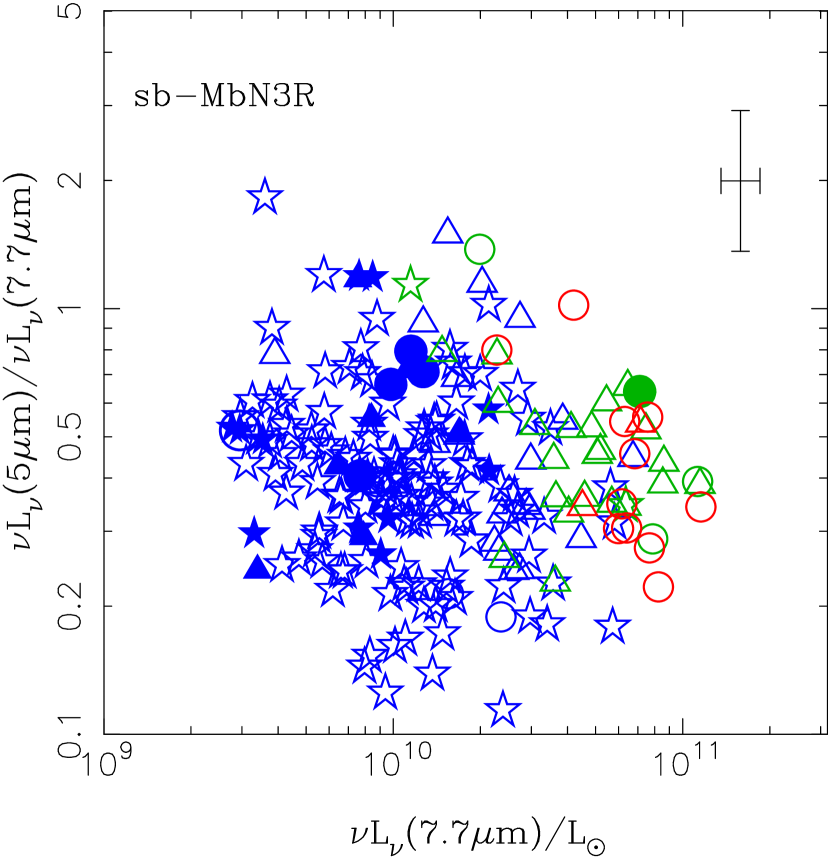
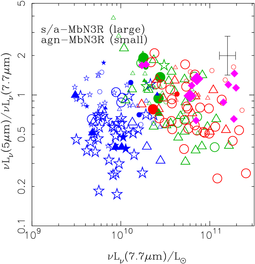
Figure 8: Correlation between the monochromatic luminosity $\nu L_{\nu\;7.7}$ at the rest-frame 7.7-$\mu\mbox{m}$ and the ratio of monochromatic luminosities. Symbols are the same as figure 6 except for their colors and sizes. The blue, green, and red symbols represent the redshifts of $0.4\leq z<0.8$, $0.8\leq z<1.2$, and $z\geq 1.2$, respectively. Small symbols represent the agn-MbN3Rs classified with the IR SED fitting. Top: Ratio of the monochromatic luminosity $\nu L_{\nu\;10}$ at the rest-frame 10 $\mu$m to the $\nu L_{\nu\;7.7}$. Bottom: The ratio of the monochromatic luminosity $\nu L_{\nu\;5}$ at the rest-frame 5 $\mu$m to the $\nu L_{\nu\;7.7}$ for the MbN3Rs. Left: For the sb-MbN3Rs. Right: For the s/a- and the agn-MbN3Rs. Large and small symbols represent the s/a- and agn-MbN3Rs, respectively.

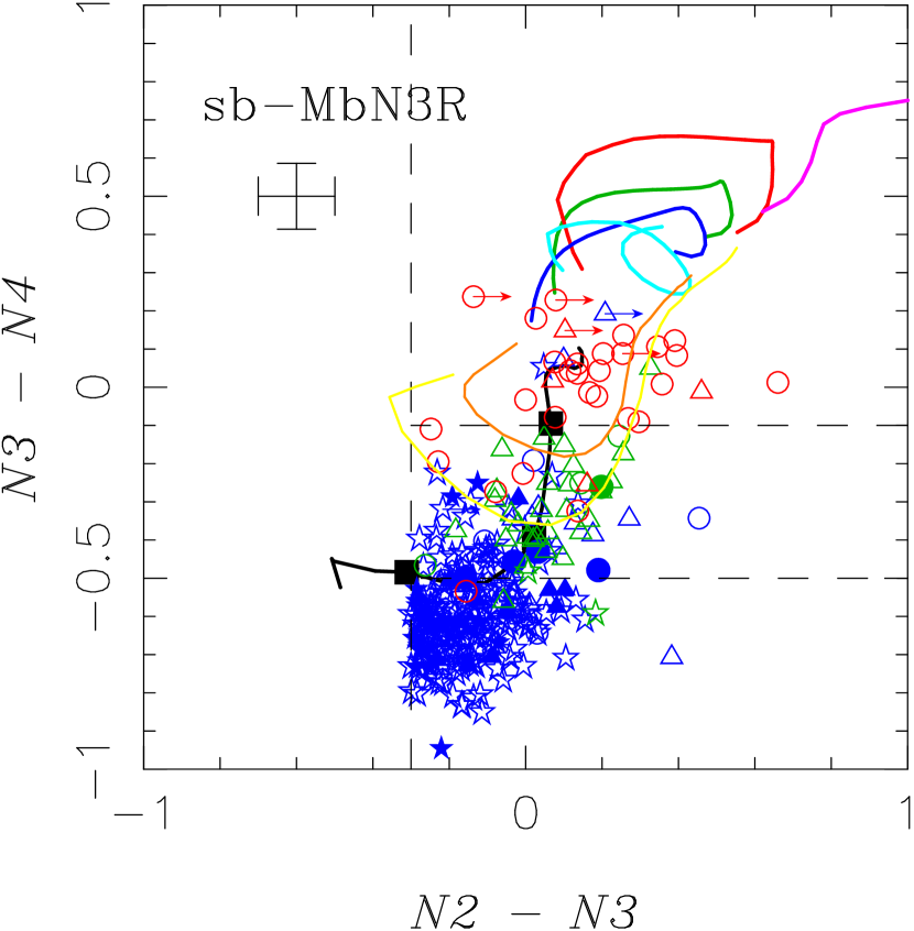
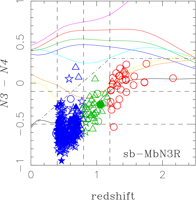
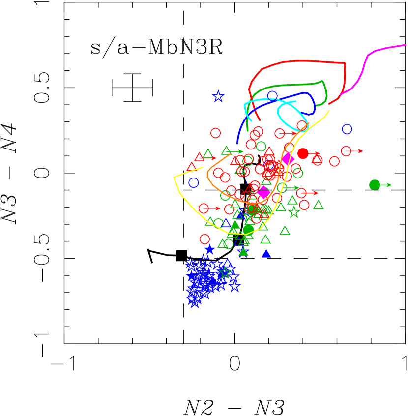
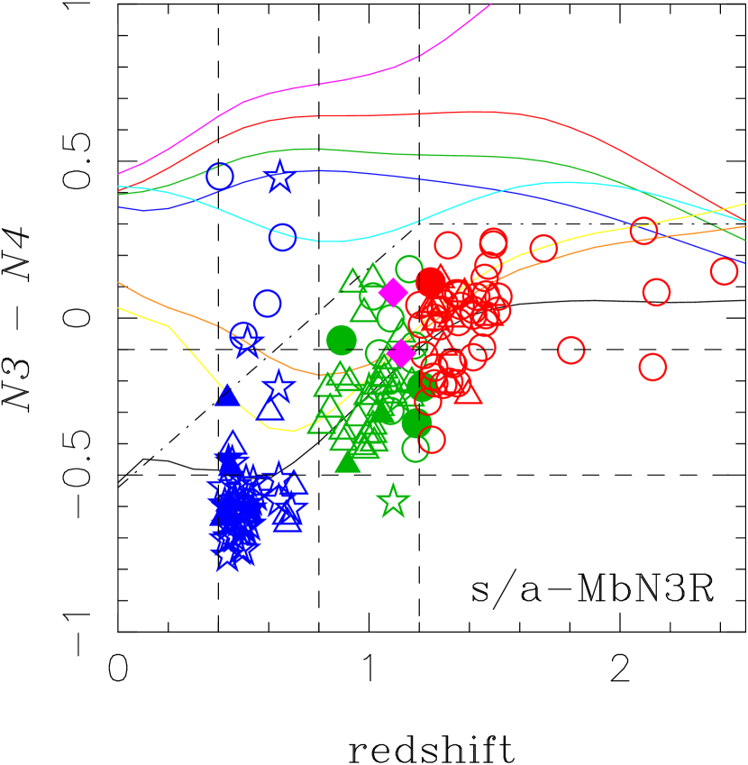
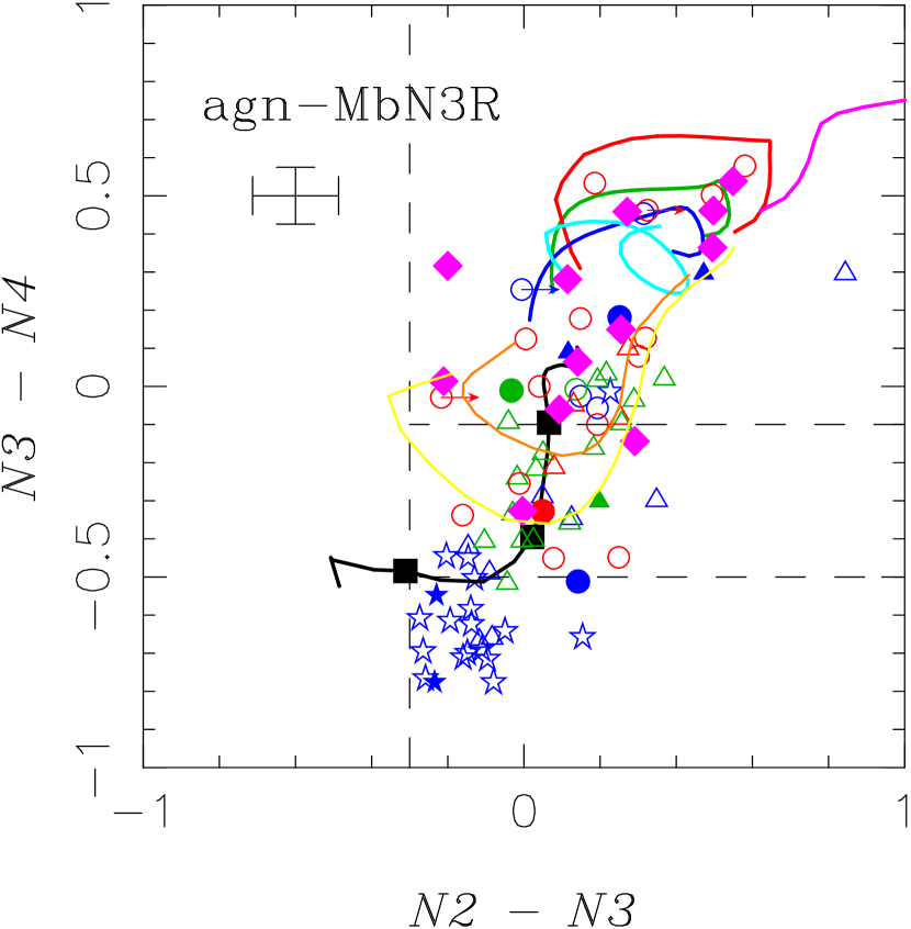
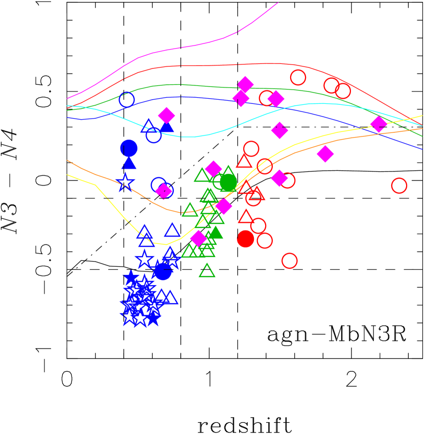
Figure 9: Left: The same as figure 3 for the MbN3Rs. Symbols are the same as figure 6 except for their colors. Blue, green, and red symbols represent objects at the redshifts of $0.4\leq z<0.8$, $0.8\leq z<1.2$, and $z\geq 1.2$, respectively. Right: Redshift vs. $N3-N4$ color. Top: For the sb-MbN3Rs. Middle: For the s/a-MbN3Rs. Bottom: For the agn-MbN3Rs.

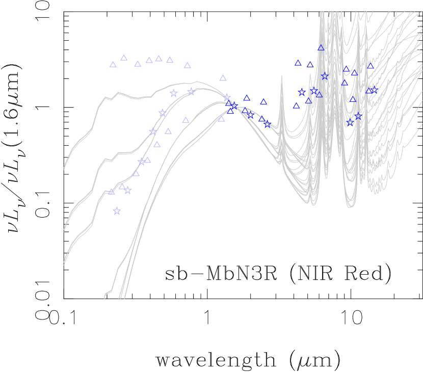
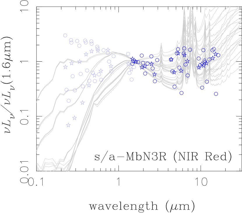
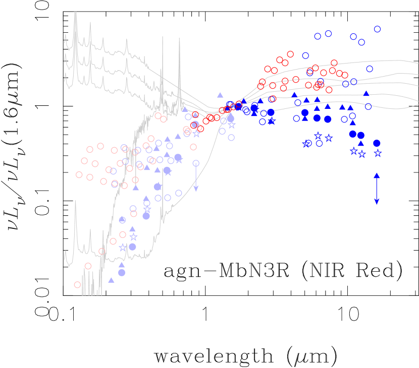
Figure 10: The same as figure 7 for the MbN3N4Rs. Left: For the sb-MbN3N4Rs. Middle: For the s/a-MbN3N4Rs. Right:For the agn-MbN3N4Rs.

The AKARI/IRC MIR photometry, in the $S7$, $S9W$, $S11$, $L15$, $L18W$, and $L24$ bands, is capable of tracing the features of PAH emissions at 3.3, 6.2, 7.7 and 11.3 $\mu$m and Si absorption at 10 $\mu$m (rest-frame) from dusty starbursts in the MbN3Rs. The MIR two-color diagrams of $S9W-S11$ vs. $S11-L15$ ($S9W/S11/L15$) and $S11-L15$ vs. $L15-L18W$ ($S11/L15/L18W$) are useful to trace the redshifted PAH features as the strong PAH 7.7 $\mu$m emission (the dip between PAH 6.2 and 7.7 $\mu$m) enters into the $L15(S11)$ band for higher-redshifted dusty starbursts in a redshift range of $z=0.4-2.6$. In order to characterize MIR SED features for the MbN3Rs, we present their observed colors on two-color diagrams of $S9W/S11/L15$ and $S11/L15/L18W$ as shown in figure 6. In order to classify them in the MIR two-color diagram. we have selected $\sim 600$ MbN3Rs from the N3Rs with the detection of $SN>3$ in the MIR bands.

Dusty starburst MbN3Rs (s-MbN3Rs) are distinguished from AGN dominated ones (agn-MbN3Rs) with solid lines in figure 6 as the boundary between the two populations, which are derived from the redshifted tracks of their MIR SEDs (see figure 63 in the appendix). On the other hand, the agn-MbN3Rs are selected with MIR color criteria in each of the redshift interval classes, which are

$$(S9W-S11)<0.3\;\cap\;(S11-L15)>0.0$$ (8)

at $z=0.4-1.0$,

$$(S9W-S11)<0.3\;\cap$$

$$\;(S11-L15)<-1.5(S11-L15)+1.2$$ (9)

at $z=0.8-1.4$,

$$(S11-L15)<0.8\;\cap\;(L15-L18W)<0.3$$ (10)

at $1.0<z<2.8$. Assuming that the MbN3Rs are at photometric redshift $z_{phot}$ derived in subsection 4.1, the classification criteria at $z=0.4-1.0$, $z=0.8-1.4$, and $1.0<z<2.8$ are applied for the MbN3Rs with the photometric redshifts of $0.4\leq z_{phot}<0.8$, $0.8\leq z_{phot}<1.2$, and $1.2\leq z_{phot}$, respectively, as shown in figure 6. The three redshift intervals roughly correspond to N3 Red uVis (N23 bumpers), uRJs (N34 bumpers), and BzKs (N4Rs) in N3 Red BBGs (IRBGs), respectively. Even with substitution of the photometric selections as the BBGs (IRBGs) for the redshift selections, the MIR two-color diagrams can be also applied to the distinction between dusty starbursts and AGNs.

We have also fitted this AKARI/IRC photometry for the s-MbN3Rs observed at the $7-24~{}\mu$m wavelength with the SED templates of starbursts (Siebenmorgen & Krügel 2007) (hereafter S&K model, see also appendix E.4). Even though we can roughly distinguish s-MbN3Rs and agn-MbN3Rs only with the AKARI MIR colors as their MIR emissions are dominant from dusty starburst and AGN, some AGNs may still coexist with dusty starbursts as hidden in the s-MbN3Rs. In order to classify the s-MbN3Rs into two subgroups of starburst dominants and starburst$/$AGN coexisting, we performed the MIR SED fitting with composite SED models, in which the dusty torus model in the SWIRE library is added to the dusty starburst S&K model with the mixing rates of $10,20,30,40,50,60,70,80,90$, and $100\%$ in the rest-frame 5-$\mu$m luminosity. We have selected sb-MbN3Rs and s/a-MbN3Rs with the mixing rates of the dusty torus $<50\%$ and $\geq 50\%$ as starburst-dominants and starburst/AGN coexisting, respectively, derived from the MIR SED fitting. The MIR SED fitting results for the MbN3Rs are consistent with their simple MIR color classification as MbN3Rs fitted well with the high AGN mixing rate which overlaped with the agn-MbN3Rs classified by the MIR color. Figure 7 shows the SEDs normalized at 1.6 $\mu$m for sb-, s/a-, and agn-MbN3Rs where we had estimated the rest-frame monochromatic magnitudes (luminosities) with their spectroscopic and photometric redshifts. For the photometric sb-, s/a-, and agn-MbN3Rs, their averaged MIR SEDs are also derived as shown with black lines on the right side.

Rest-frame SEDs of the sb-MbN3Rs, as shown in figure 7, show deep dips around 5 and 10 $\mu$m and a strong excess around 8 $\mu$m with weak ones around 3 and 11 $\mu$m. The features agree well with SEDs of dusty starburst S&K models overplotted as thin lines. It indicates not only the consistency for this starburst classification with MIR colors and MIR SED fittings but also accuracy for their photometric redshifts. On the other hand, the features are not so clear for the agn-MbN3Rs. The 5 $\mu$m dip corresponds to the transition between the stellar emission and the dust emission from their star-forming regions. The strong excess around 8 $\mu$m with weak ones around 3 and 11 $\mu$m and the dip around 10 $\mu$m can be also naturally explained with the PAH 7.7, 3.3, and 11.3 $\mu$m emissions and Si 10 $\mu$m absorption in typical MIR emission from their dusty star-forming regions.

Figure 8 shows similar trends to those which appeared in figure 7 as the dips at rest-frame 5 and 10 $\mu$m are deeper in the sb-MbN3Rs than in the s/a- and agn-MbN3Rs. The trends can be also naturally explained as MIR SEDs of s/a-MbN3R consist of a smooth power-law or convex component adding to an original component with deep concave dips at 5 and 10 $\mu$m, which agree well with the superimposed SEDs composed of dusty starburst S&K models and the dusty torus model in the SWIRE SED library with the ratio of 0.3 to 0.7 at 5 $\mu$m. The composition of starburst and dusty torus is typically characterized by the monochromatic luminosity ratio of s/a-MbN3Rs shown in figure 8. This is consistent with a picture of an obscured AGN coexisiting with dusty star-forming region in an s/a-MbN3R which contributes to the additional smooth component and the emission with the 5 and 10 $\mu$m dips in the MIR SED, respectively.

6.2 NIR colors of MbN3Rs

The NIR color diagram of figure 9 for the MbN3Rs can also support the existence of the dusty torus hidden in the agn- and s/a-MbN3Rs with the excess in the $N4$ band. The agn- and s/a-MbN3Rs even at $z<1$ appear in the region of $N3-N4>-0.1$, which is the same trend as for the BL AGNs and expected from the tracks of the dusty torus and QSO models as shown in figure 9. For stellar compornent with the IR bump, the mean $N3-N4$ color track, represented as solid lines in the right plots of figure 9, can be roughly approxinated as a function $N3N4(z)$ of $z$:

$$N3N4(z)=\left\{\begin{array}[]{ll}0.74z-0.84&(0.4\leq z<1.2)\\ 0.048&(z\geq 1.2)\end{array}\right.\;.$$ (11)

Thus, we have selected AGN candidates with an NIR color criterion:

$$N3-N4>N3N4(z)+\Delta N34\;,$$ (12)

where we have taken a typical $N3-N4$ color error $\Delta(N3-N4)$ into account and introduced $\Delta N34=3\Delta(N3-N4)$. The galaxies, selected with this additional NIR color criterion from the N3Rs, will be called N3N4 Red galaxies (N3N4Rs). The boundary of the NIR color criterion is shown as dotted dash lines in the right plots of figure 9, where $\Delta(N3-N4)=0.1$ as a typical $N3-N4$ color error for the MbN3Rs, which selects MIR bright N3N4Rs (MbN3N4Rs). As shown in figure 10, the SEDs of agn- and s/a-MbN3N4Rs are similar to spectroscopically confirmed BL AGNs in agn-MbN3Rs. The redder color $N3-N4$ in the agn- and s/a-MbN3N4Rs is consistent with the existence of a dusty torus, which dominates stellar components of the host. On the other hand, the SEDs of sb-MbN3N4Rs are still similar to those of dusty starbursts as most of the sb-MbN3Rs. The sb-MbN3N4Rs, even with the redder color $N3-N4$, may be still dusty starburst dominant. Thus, the MIR SED classification for the sb-MbN3Rs is robust to distinguish dusty starbursts from AGNs while the NIR color classification can be effective only to select bright obscured AGNs.

6.3 MIR marginally-detected N3Rs

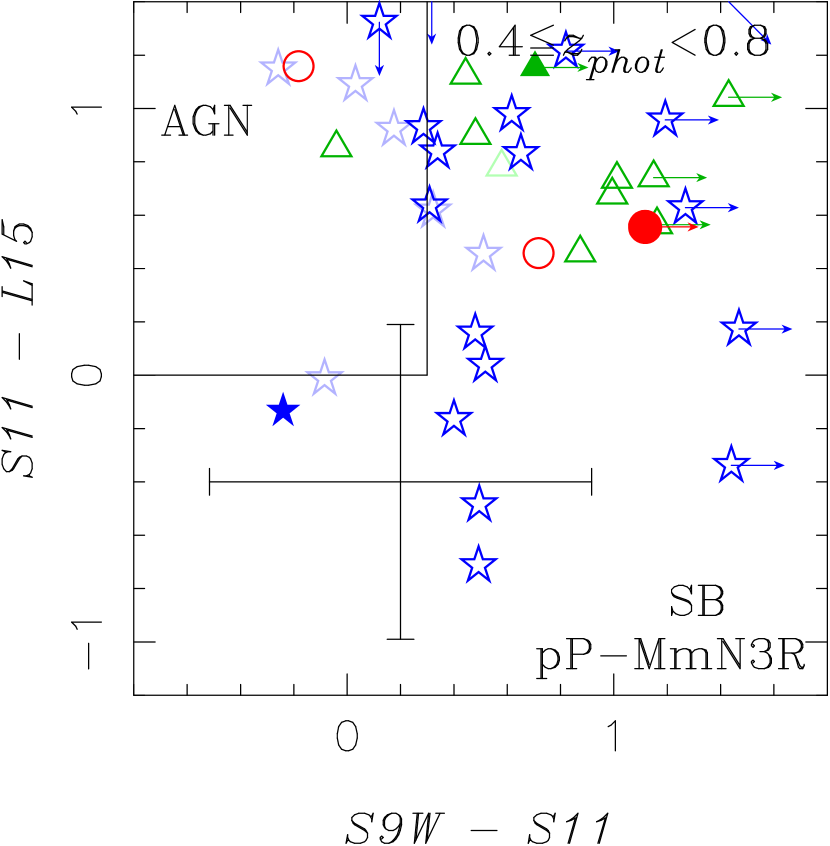
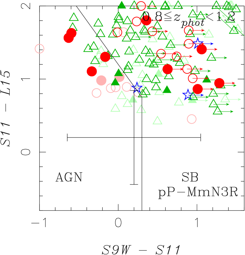
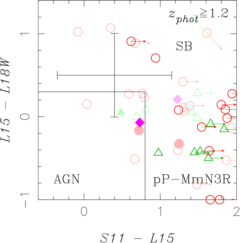
Figure 11: The same as figure 6 for the pP-MmN3Rs. Dark and faint symbols represent the sb- and non sb- pP-MmN3Rs, respectively.

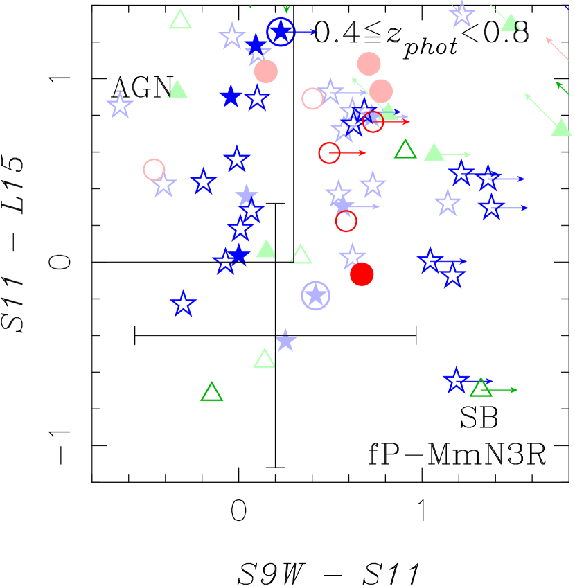
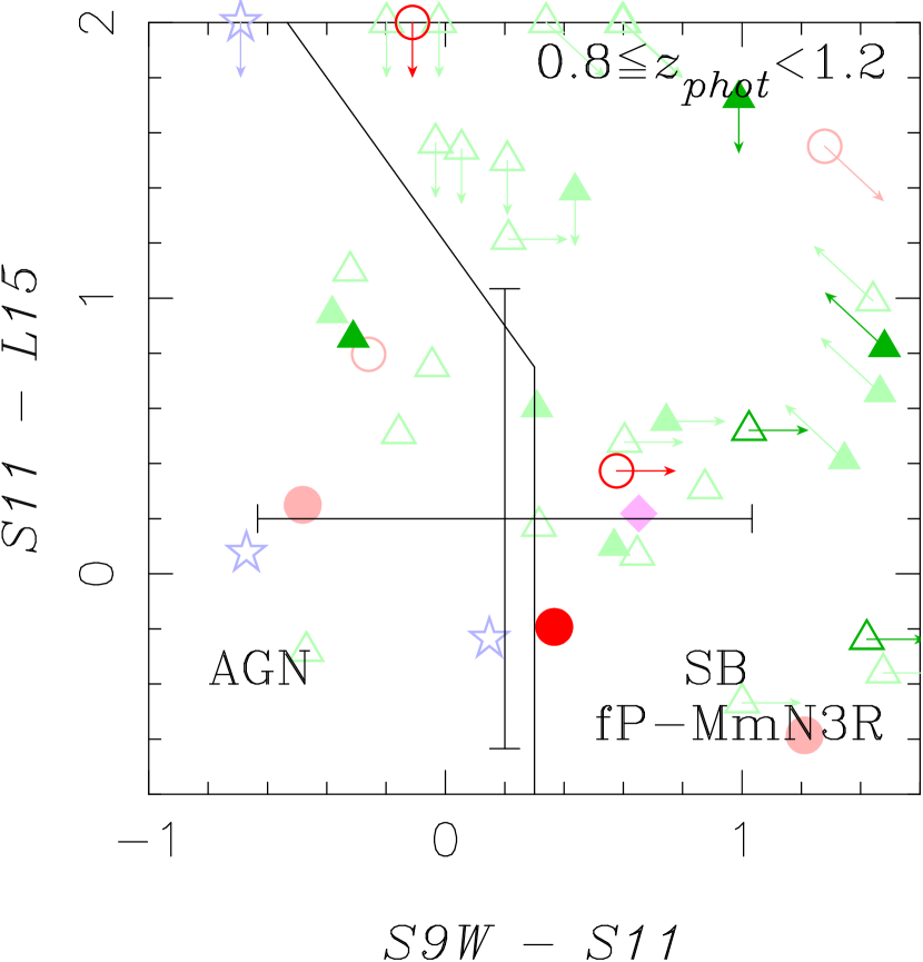
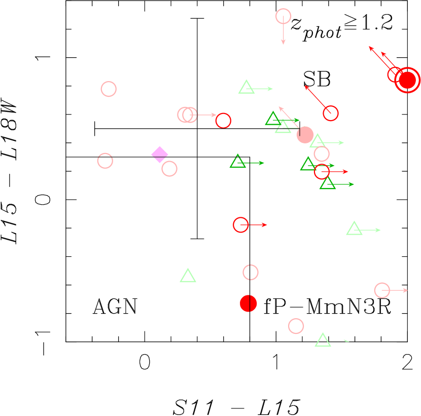
Figure 12: The same as figure 11 for the fP-MmN3Rs. Dark and faint symbols represent sb- and non sb-fP-MmN3Rs, respectively.

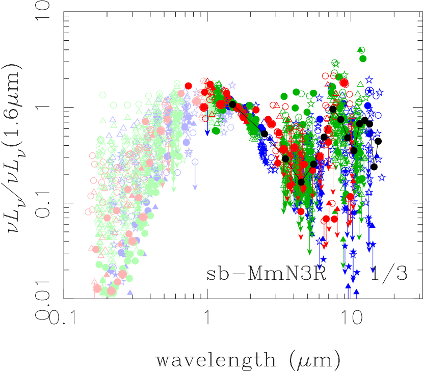
Figure 13: The same as figure 7 for the MmN3Rs. Left: For the sb-MmN3Rs. Right: For the non sb-MmN3Rs.

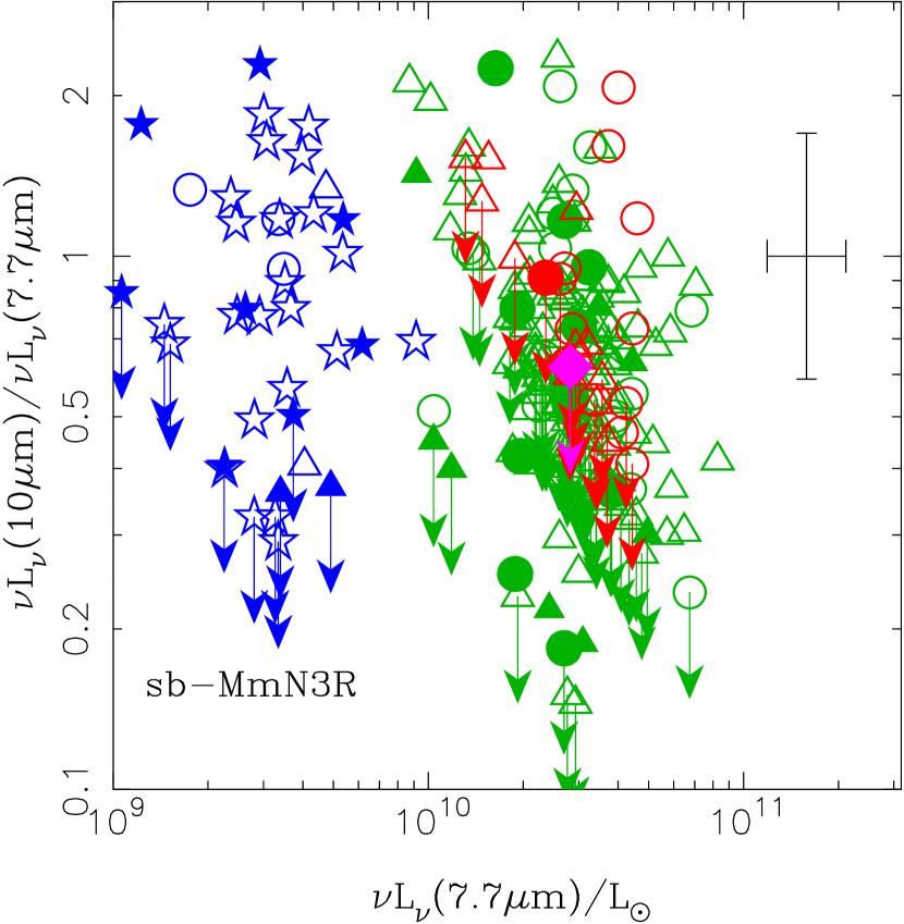
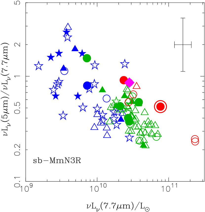
Figure 14: The same as figure 8 for the sb- and non sb-MmN3Rs.

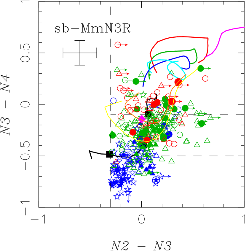
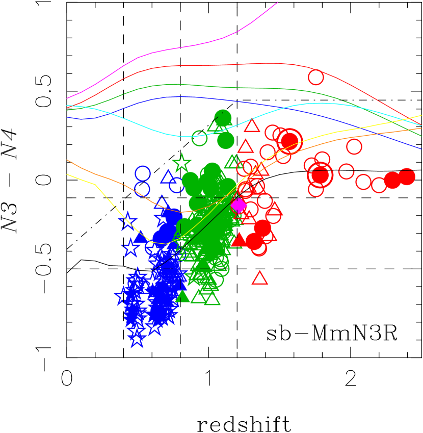
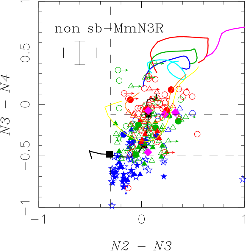
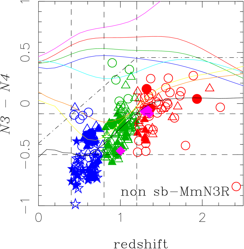
Figure 15: The same as figure 9 for the MmN3Rs.

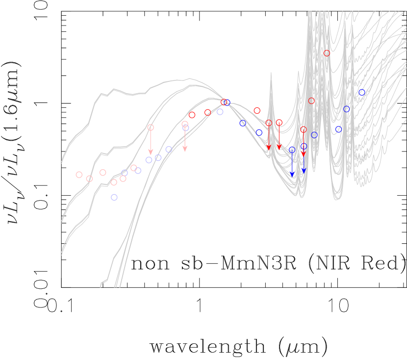
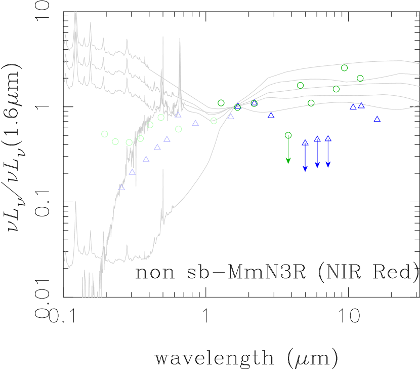
Figure 16: The same as figure 7 for the MmN3N4Rs.

We should remark that the MIR multi-band photometry with the IRC can select unique samples for studying star formation and AGN activity as not only the MbN3Rs but also sources detected only in some of the S7, S9W, S11, L15, L18W, and L24 MIR bands. As shown above, the S11, L15, L18W, and L24 of the IRC are effective in detecting the 7.7 $\mu$m PAH emission from dusty starbursts at $z\geq 0.4$. Even though we have selected $\sim 600$ MbN3Rs with the detection of $SN>3$ in more than two MIR bands in subsection 6.1, we have also excluded MIR sources in the N3Rs as detected only in one or two MIR bands with detection of $SN>3$ and in other MIR bands with detection of $SN<3$, which are called MIR marginally-detected N3Rs (MmN3Rs), whose MIR magnitudes and colors can be still estimated as the MmN3Rs are mimics of the MbN3Rs. We selected $\sim$600 MmN3Rs, which are subclassified into $\sim$320 possible PAH emitting (pP-)MmN3Rs and $\sim$270 faint PAH emitting (fP-)MmN3Rs. The former can be PAH 7.7 $\mu$m emitters as detected in the S11, L15, and L18 bands at $z=0.4-0.65,0.65-1.5$, and $>1.5$, respectively, while the latter even have MIR emission but possibly not related to the PAH emissions. Thus, the pP-MmN3Rs and fP-MmN3Rs could be candidates for dusty starbursts and AGN mixtures or less-active star-forming with and without the PAH emissions in their selection criteria, respectively.

Following the MIR color classifications in subsection 6.1, we checked the difference between the pP- and fP-MmN3Rs on the MIR color-color diagrams as shown in figures 11 and 12. Even though the errors in the MIR colors of the MmN3Rs are large, most of the pP-MmN3Rs appear in the area of dusty starburst in the MIR color-color diagrams, which are similar to the s-MbN3Rs. On the other hand, the fP-MmN3Rs are more dispersed on the diagrams, which suggests that the fP-MmN3Rs mainly consist of star-forming and AGN mixtures. In order to classify the MmN3Rs into two subgroups of starburst and non starburst, we also performed the MIR SED fitting with the same composite SED models as described in subsection 6.1. We selected sb- and non sb-MmN3Rs with the mixing rates of the dusty torus $<50\%$ and $\geq 50\%$ in MIR SED fittings as starburst-dominants and possibly non starburst, which are represented as dark and thin symbols, respectively, in figures 11 and 12. Then, we categorized these starburst dominant MmN3Rs (sb-MmN3Rs) as mimics of sb-MbN3Rs.

In fact, $\sim 240$ out of $\sim 320$ pP-MmN3Rs are sb-pP-MmN3Rs, while only $\sim 110$ out of $\sim 270$ fP-MmN3Rs are sb-fP-MmN3Rs. Thus, the classifications from the MIR colors for pP-MmN3Rs and fP-MmN3Rs are roughly consistent with those from the MIR SED fittings for sb-MmN3Rs and non sb-MmN3Rs. Figure 13 also shows averaged MIR SEDs of sb-MmN3Rs and non sb-MmN3Rs. We can see that the averaged MIR SED of the sb-MmN3Rs have dusty starburst features with deep dips around 5 and 10 $\mu$m and excesses around 8 and 11 $\mu$m in the SEDs, which are similar to the sb-MbN3Rs as shown in figure  7. We can also see these features in the luminosity ratios of $\nu L_{\nu,10}/\nu L_{\nu,7.7}$ and $\nu L_{\nu,5}/\nu L_{\nu,7.7}$ as shown in figure 14. On the other hand, the averaged MIR SED and the luminosity ratio of the nonsb-MmN3Rs are similar to those of the s/a-MbN3Rs. We also tried to find AGN candidates hidden in the MmN3Rs with the NIR color criterion of equation (12) as applied in the MbN3Rs in subsection 6.1. With $\Delta(N3-N4)=0.15$ as a typical $N3-N4$ color error for the MmN3Rs, the boundary of the criterion is represented again as dotted-dashed lines in figure 9, which select MmN3N4Rs. As shown in figure 16, the sb- and nonsb-MmN3N4Rs are similar to the sb- and agn-MbN3N4Rs, respectively.

Thus, the distinction between starbursters and AGNs with features in MIR/NIR SED is basically valid even in the MmN3Rs the same as the MbN3Rs. Thus, we can treat sb-MmN3Rs as mimics of s-MbN3Rs in the following sections.

6.4 MIR faint N3Rs and BBGs

From the opposite point of view to subsections 6.1 and 6.3, weak emission or non-detection in these MIR IRC bands are still important constraints for selecting galaxies with low extinction or AGNs with weak dusty torus emission. These MIR faint sources, having less than the limiting magnitudes of those in table 2 in all the MIR bands (S9, S11, L15, L18W, and L24), can be classified into a subclass population of N3Rs, which we call as MIR faint N3Rs (MfN3Rs) as alternatives to not only the MbN3Rs but also the MmN3Rs. The MfN3Rs may in general also consist of star-forming and passive populations in the BBGs with weak dust emission. For example, passive uVis, uRJs, and BzKs without the 7.7 $\mu$m PAH emission at $0.4\leq z<0.8$, $0.8\leq z<1.2$, and $1.2\leq z$ are expected to be faint in the S11, S11/L15, and L15/L18W bands, respectively. Thus, the MfN3Rs can be subclassified into s-and p-BBGs with the two-color diagram.

The MfN3Rs at $z>1.2$ form a limited sample in our shallow survey depth in the $J,K$ and $N3$ bands, and they are mostly identical to MIR faint BBGs (MfBBGs), MfN3Rs at $z<1.2$ are a part of MIR faint uVis (MfuVis). In order to study the evolution and mass dependence in star formation, these MfN3Rs and MfBBGs are also important as reference samples compared with the MbN3Rs and MmN3Rs for analyzing their evolutionary features of SFR, extinction, and $M_{\ast}$ in section 8. We will sometimes refer to MfBBGs as MfBBGs not classified as MfN3Rs in the following.

6.5 Comparison with X-ray and Radio Observations

Before closing this section, we will quickly compare the MIR SED classification with recent results at X-ray and radio wavelengths. AGNs being harbored in the agn-MbN3Rs and the s/a-MbN3Rs are also indicated from a preliminary look at our recent Chandra X-ray Observatory (CXO) data on this field (Krumpe et al. in prep.; Miyaji et al. in prep), which show that $\sim$50% of the agn-MbN3Rs and $\sim$15% of the s/a-MbN3Rs have counterparts of X-ray sources. Thus, the trend for the X-ray sources also support that the MIR SED classification is effective for selecting AGNs. Furthermore, as shown in figure 13, the nonsb-MmN3Rs are possibly harboring AGNs with dusty starbursts. If it is true, their X-ray emission can be detected with stacking analysis of their CXO data. Thus, the CXO data can be effective to study AGN activities not only for the MbN3Rs but also for the MmN3Rs.

We have also made a radio observation with the WSRT at 1.4 GHz of $\simeq 1.7$ deg² covering the field, which found $\simeq 500$ sources with $>0.1$ mJy in the field  (White et al. 2010). The radio source counts are consistent with a two population model with radio loud sources and radio faint sources with $<$ 1 mJy, in which it was assumed that the former and the latter are powered by AGNs and star-forming galaxies as in previous studies of other deep fields. The radio loud and the sub-mJy populations possibly overlap with the agn- and s-MbN3Rs, respectively. However, as the s-MbN3Rs were subclassified to the starburst dominates (sb-MbN3Rs) and the starburst/AGN co-existence(s/a-MbN3Rs) in subsection 6.1, the sub-mJy radio populations can be also subclassified to starburst dominant and starburst/AGN co-existence populations. Thus, it will be interesting to compare the MIR populations with the X-ray and radio sources, which will be studied in a future paper.

7 Calorimetric studies with MIR SEDs

For the s-MbN3Rs and the sb-MmN3Rs classified as dusty starbursts, their MIR SEDs with PAH emissions and Si absorption should contain rich information not only as distinguished from AGNs but also about the physical properties in their star-forming regions such as their bolometric luminosities, SFRs, and extinction, which were derived by calorimetric schemes in MIR SED analysis.

7.1 Bolometric Luminosity and SFR

As long as AGN activity is negligible in a galaxy, young stars are dominant sources for the emission. Thus, the contribution of SFRs are nearly equal to the bolometric luminosity for star-forming galaxies. We can estimate the total emitting power with an SED analysis for multi-wavelength photometric data and convert it to the SFR. SFRs are derived not only from intrinsic UV continuum luminosity by assuming an extinction law for all the $z^{\prime}$-detected galaxies, but also from IR luminosity for the s-MbN3Rs and the sb-MmN3Rs.

When massive stars are not obscured by dust, SFR on a star-forming region can be directly traced with their UV continuum luminosity in the rest-frame wavelength 1500$\AA$. Thus, the UV luminosity can be translated into the SFR by the relation:

$$SFR_{UV}\left[\mbox{M}_{\odot}{\rm yr}^{-1}\right]=\frac{L_{\nu}(1500\mbox{\AA})}{8.85\times 10^{27}[{\rm erg\ s^{-1}Hz^{-1}}]}\;.$$ (13)

When massive stars are born in dust obscured star-forming regions, their UV radiation is reprocessed into IR emission. In this case, the SFR can be traced mainly with their TIR luminosity $L_{IR}$. Even without using their TIR luminosity, as frequently applied, the intrinsic UV continuum luminosity $L_{UV;cor}$ can be reconstructed with a correction for the classical dust extinction $A_{UV;opt}$ from the observed UV luminosity $L_{UV;obs}$ (see also the details in subsection 7.3), and derive $SFR_{UV;cor}$ from $L_{UV;cor}$ with equation (13) and/or directly optical-NIR SED fittings with synthesis models. The scheme for $SFR_{UV;cor}$ can be applied even for all the $z^{\prime}$-detected galaxies including MIR faint galaxies.

For the s-MbN3Rs and the sb-MmN3Rs, on the other hand, with integrating a fitted model SED from 8 to 1000 $\mu$m in the rest-frame with correcting for the photometric redshift $z_{phot}$, we can obtain the total IR (TIR) luminosity $L_{IR}$ of the emission from the dusty star forming regions. According to Kennicutt (1998), thus, the SFR can be estimated from $L_{IR}$ as

$$SFR_{IR}\left[\mbox{M}_{\odot}\mbox{yr}^{-1}\right]=\frac{L_{IR}}{2.2\times 10^{44}\left[\mbox{erg s}^{-1}\right]}\;,$$ (14)

where we assumed the Salpeter IMF in the optical-NIR SED fitting as shown in subsection 4.1. In general, the total SFR in a galaxy is derived as a sum:

$$SFR_{IR+UV}=SFR_{IR}+SFR_{UV;obs}\;,$$ (15)

since dust can partially obscure galaxies. It is noted that ${\rm SFR}_{UV;obs}$ is derived from the observed UV luminosity $L_{UV;obs}$ without extinction correction.

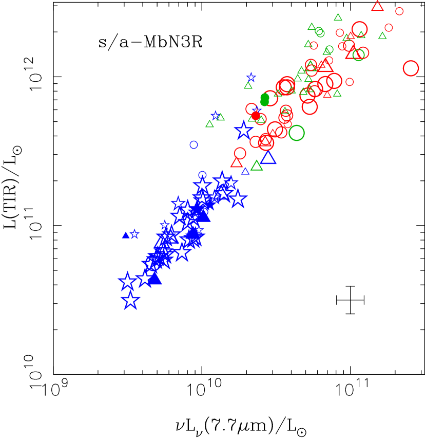
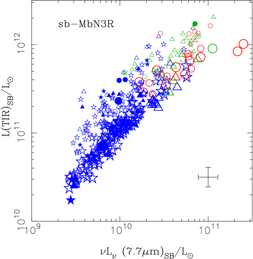
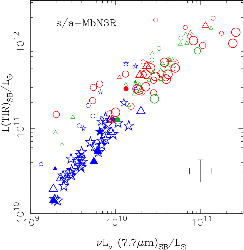
Figure 17: Rest-frame 7.7-$\mu$m monochromatic luminosity $\nu L_{\nu\;7.7~{}\mu\mbox{m}}$ vs. the TIR luminosity $L_{IR}$ derived from the IR SED fittings for the s-MbN3Rs. Symbols are the same as in figure 6 except for their colors and sizes. Blue, green, and red symbols represent objects at the redshifts of $0.4\leq z<0.8$, $0.8\leq z<1.2$, and $z\geq 1.2$, respectively. Large, medium, and small symbols indicate the results which fit well with the S&K model SEDs of $A_{V;SK}=2.2,6.7$, and $17.9$, respectively. Top: The $L_{IR}$ derived without excluding the contribution from the hidden AGN. Bottom: The $L_{IR}$ derived with excluding the contribution from the hidden AGN. Left: For the sb-MbN3Rs. Right: For the s/a-MbN3Rs.

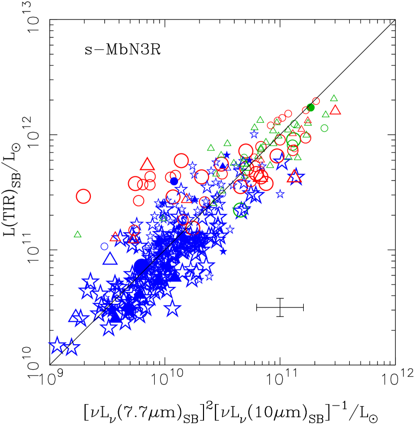
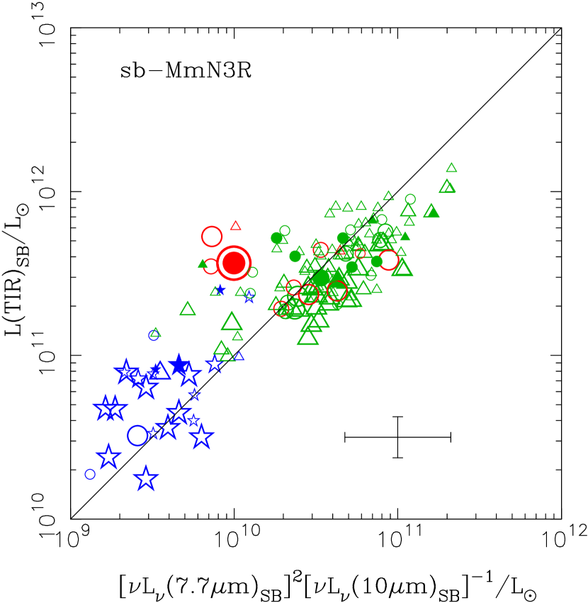
Figure 18: Relation between TIR luminosity $L_{IR}$ estimated from the S&K model and the rest-frame luminosities of $L_{\nu;7.7~{}\mu m}$ and $L_{\nu;10~{}\mu m}$. Symbols are the same as in figure 6 except for their colors and sizes. Blue, green, and red symbols represent objects at the redshifts of $0.4\leq z<0.8$, $0.8\leq z<1.2$, and $z\geq 1.2$, respectively. Large, medium, and small symbols indicate the results which fit well with the S&K model SEDs of $A_{V;SK}=2.2,6.7$, and $17.9$, respectively. The line represents the relation approximated with equation (16).

7.2 Total IR Luminosities from MIR SED

By means of the S&K models as a library of SED templates required in MIR SED fittings, we could derive TIR luminosity from the fitted IR SEDs for the s-MbN3Rs. Thus, we could obtain a relation between the rest-frame monochromatic 7.7 $\mu$m luminosity $\nu L_{\nu 7.7}$ and the TIR luminosity $L_{IR}$ for all the s-MbN3Rs including both sb-MbN3Rs and s/a-MbN3Rs as shown in figure 17. The top and bottom diagrams in figure 17 indicates the results in the $L_{IR}$ estimation without and with the subtraction of the obscured AGN contribution, respectively. Before the subtraction of the AGN contribution, TIR luminosity range of the s/a-MbN3Rs is larger than those of the sb-MbN3Rs as shown in the top diagrams in figure 17. After the subtraction, the discrepancy in TIR luminosities between the sb- and s/a-MbN3Rs was reduced. This suggests that the subtraction is effective to derive TIR luminosities even for the s/a-MbN3Rs, which is also essential to estimate their SFRs as discussed in subsection 8.2.

Even though the TIR luminosity correlates well with the rest-frame 7.7-$\mu$m monochromatic luminosity $\nu L_{\nu 7.7}$ as shown in figure 17, this estimation of the TIR luminosity with the MIR SED fitting seems to be still a kind of extrapolation to obtain the Far InfraRed (FIR) emission around $\simeq 1000~{}\mu$m from the NIR/MIR side only up to $\simeq 24~{}\mu$m with the best-fitted model SED. However, we would like to remark that it can be more than an extrapolation scheme since the AKARI MIR multi-band photometry can certainly trace not only the PAH emission but also the Si absorption feature as already shown in figures 7 and 8. The absorption feature depends on the optical depth in galaxies and corresponds to the TIR luminosity as discussed in the following.

We can see multi-sequences in figure 17. The splitting into the multi-sequences is mainly caused by the difference in the “mean” optical depth, which can be characterized as an SED model parameter of “visual extinction” $A_{V;SK}$ at the edge of dusty starburst nucleus in the S&K model, which is indicated by the symbol size. In MIR SED fittings with the S&K model library, we have taken the model SEDs with $A_{V;SK}=2.2,6.7$, and $17.9$ corresponding to large, medium, and small symbols in figures, respectively. Even though $A_{V;SK}$ is not equivalent to the observed visual extinction $A_{V}$ assuming spherical geometry for star forming regions in the S&K model, this parameter $A_{V;SK}$ is quantitatively related to the optical depth of the observed dusty starbursts as the model MIR SEDs with larger $A_{V;SK}$ show a deeper Si $10~{}\mu$m absorption feature since it is induced with the dust self-absorption process in dense dusty regions. In fact, the s-MbN3Rs, with not only PAH emissions but also Si $10~{}\mu$m absorption, have various ratios of $\nu L_{\nu;10}/\nu L_{\nu;7.7}$ between 10 and 7.7 $\mu$m as already shown in figure 8. Then, the observed ratio $\nu L_{\nu;10}/\nu L_{\nu;7.7}$ contains the information about the “mean” optical depth related to the denseness and the size of a dusty star-forming region, which is parametrized with the $A_{V;SK}$ in the S&K models (see the details in appendix E.4).

Thus, the MIR SED fitting with the S&K model can analyze a variational degree of “mean” optical depth possibly related to the Si absorption depth. The “mean” optical depth is another influential parameter for estimating the TIR luminosity from the MIR SED fitting. Thus, it is expected that their TIR luminosity is correlated not only with the rest-frame monochromatic 7.7 $\mu$m PAH luminosity $\nu L_{\nu;7.7}$ but also with the Si absorption depth at least for the selected starburst samples of the s-MbN3Rs and the sb-MmN3Rs as

$$L_{IR;SK}\simeq 10\times\left(\frac{\nu L_{\nu 10}}{\nu L_{\nu 7.7}}\right)^{\alpha}\times\nu L_{\nu 7.7}\;,$$ (16)

where the units of $L_{IR},\nu L_{\nu 7.7}$ and $\nu L_{\nu 10}$ is $\left[\mbox{erg s}^{-1}\right]$ and $\alpha\simeq-1$. This approximate formulation can work well as shown in figure 18.

Even though the S&K models can reproduce MIR SEDs of the s-MbN3Rs and the sb-MmN3Rs well, they are produced with some simplifying assumptions such as a spherical geometry with constant dust distribution for the modeled starburst region. Even though we could confirm the accuracy of the estimation for the TIR luminosity with complementary observations at longer wavelengths than MIR as FIR and submillimeter as remarked in section 11, we have not yet obtained them in the field. At this moment, we can not rule out a possibility that the TIR luminosity $L_{IR;SK}$, estimated with the fitted S&K models, includes a systematic offset. Thus, we will introduce a factor $f_{SK}$ in the conversion from the model estimated $L_{IR;SK}$ to the real $L_{IR}$:

$$L_{IR}=f_{SK}L_{IR;SK}\;.$$ (17)

As long as the proportional factor $f_{SK}=0.3-1$, the estimation of $L_{IR}$ is consistent with previous work. For example, taking $f_{SK}\simeq 1$, we can roughly reproduce a relation $L_{IR}\simeq 17.2L_{5-8.5~{}\mu\mbox{m}}$ by Elbaz et al. (2002). We found an offset between the S&K model and the C&E model, in which the TIR luminosity with the C&E model can be reproduced with $f_{SK}\simeq 0.3$ (see figure 64 in the appendix). In the following, we take $f_{SK}=1$ as the default value.

7.3 Classical and calorimetric extinctions

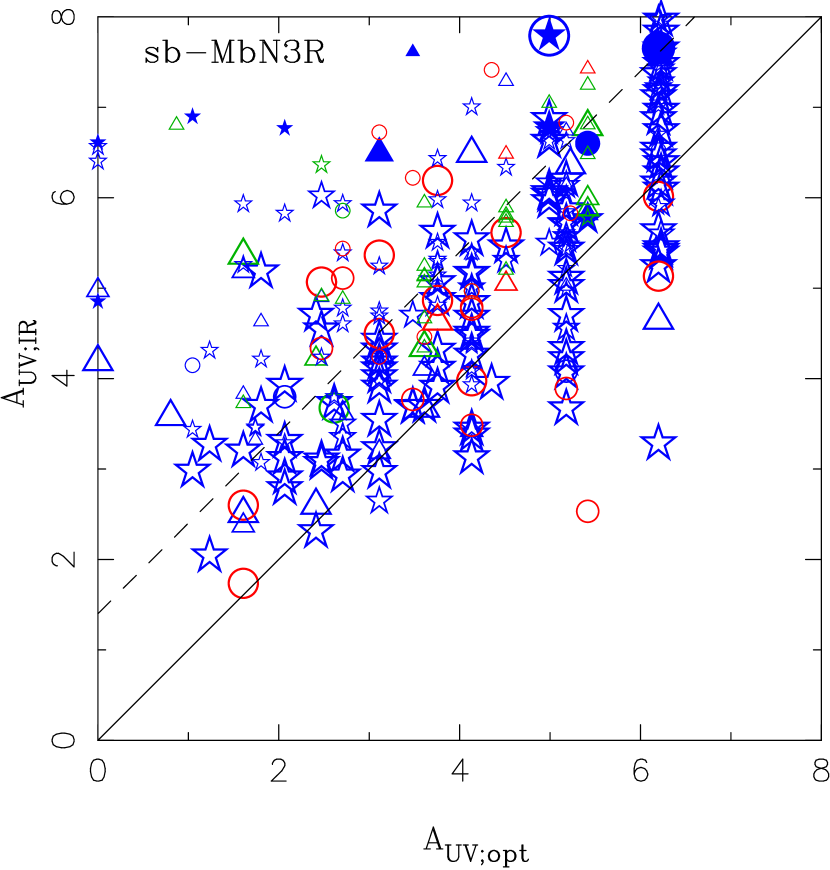
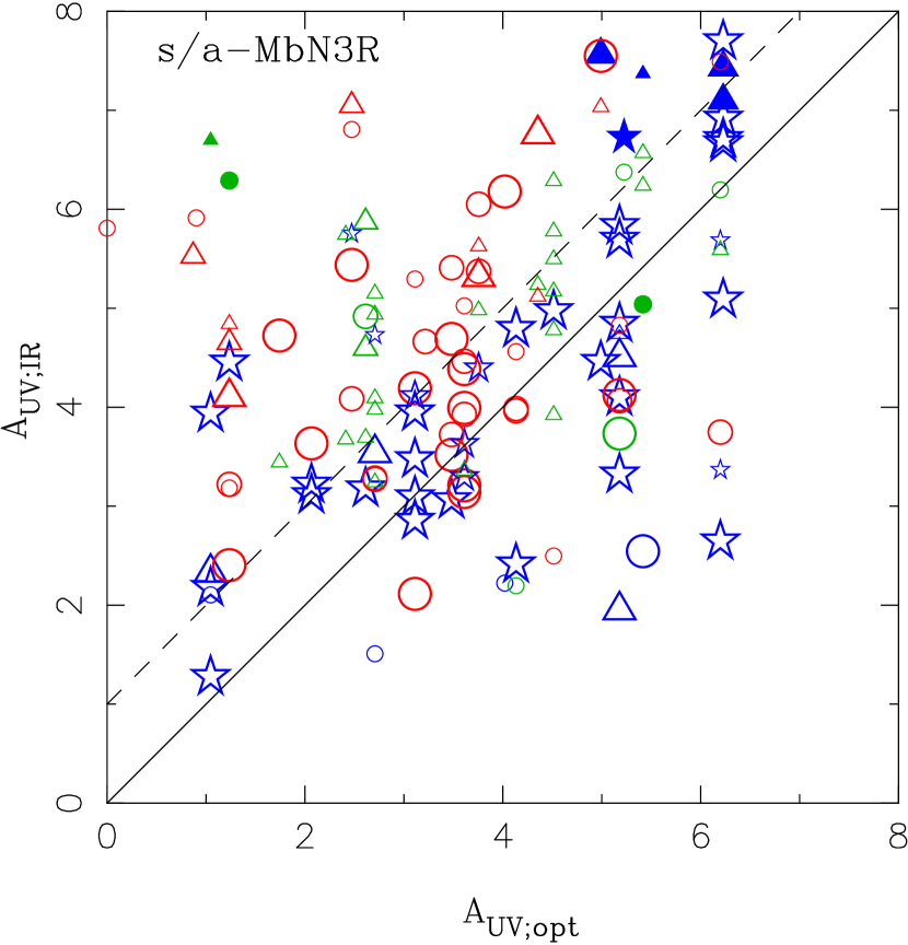
Figure 19: Correlation between two extinctions at 1500Å derived from the optical-NIR SED fitting and the luminosity ratio of the total to observed UV as $A_{UV;opt}$ vs. the $SFR_{IR+UV}/SFR_{UV,obs}$. Symbols are the same as in figure 18. Dashed line represents a proportional law with equation (21), obtained with fitting the sample. Left: For the sb-MbN3Rs. Right: For the s/a-MbN3Rs.

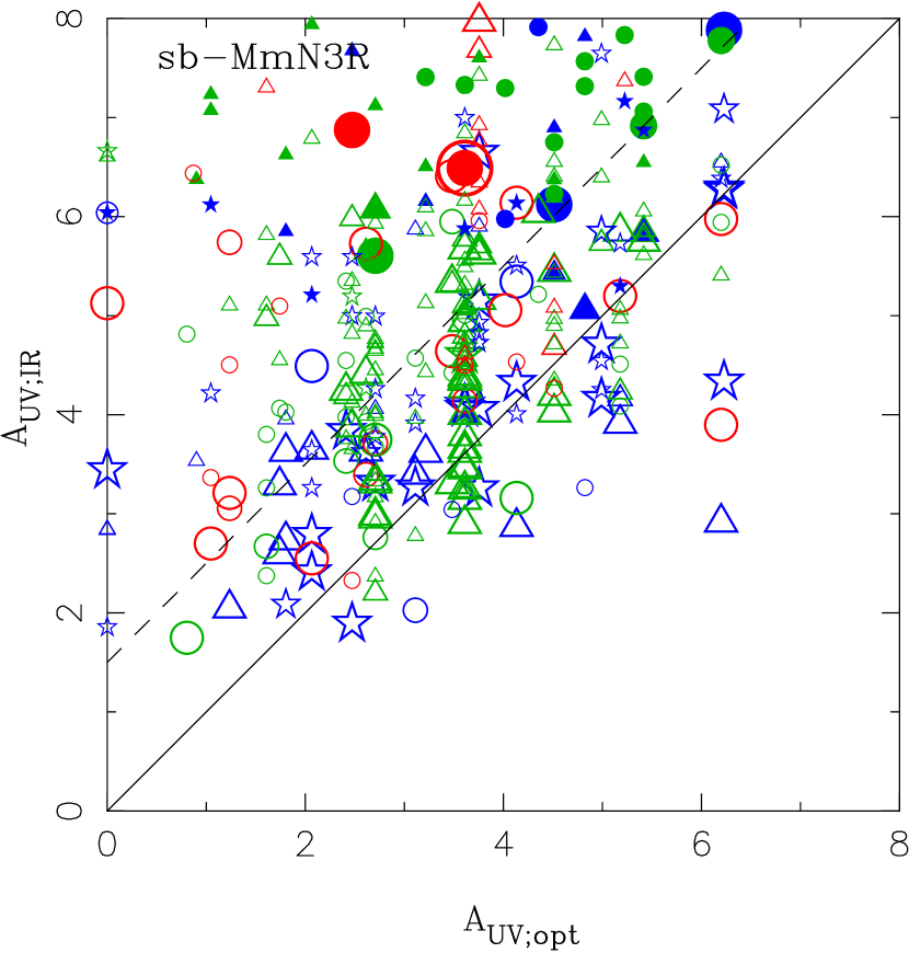
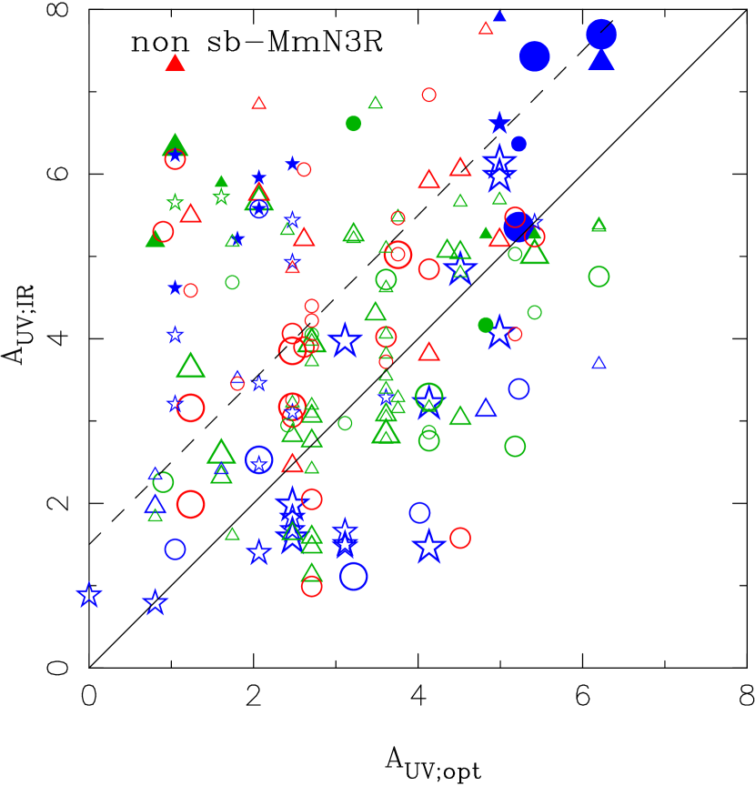
Figure 20: The same as figure 19 for the MmN3Rs. Dashed line represents a proportional law with equation (21), obtained with fitting the sample. Left: For the sb-MmN3Rs. Right: For the nonsb-MmN3Rs.

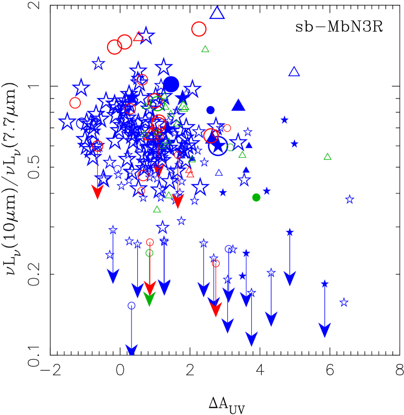
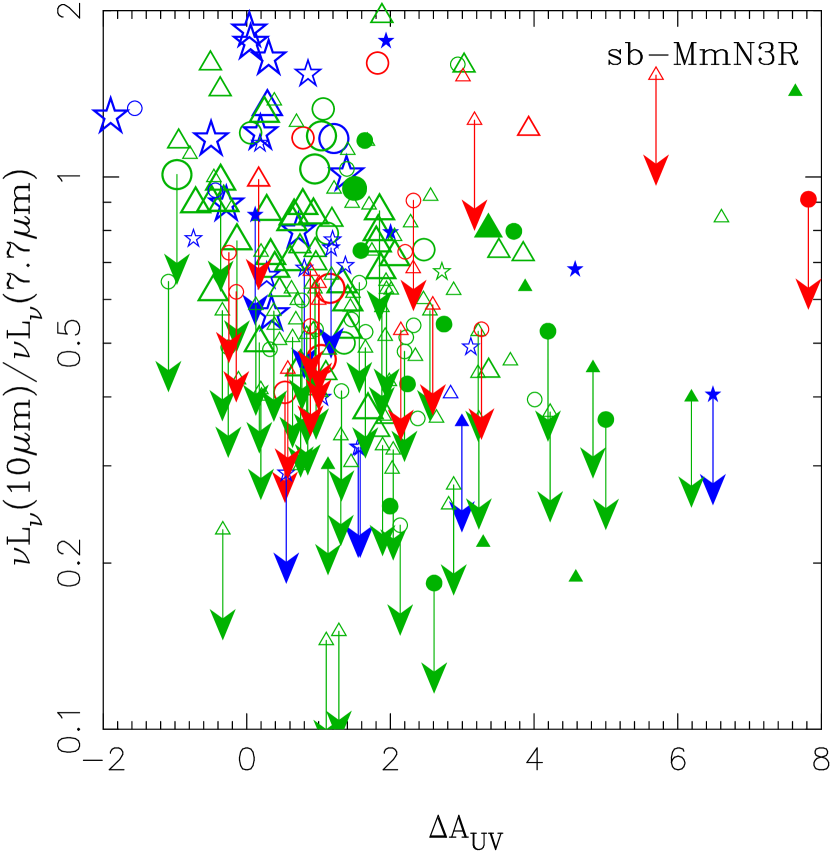
Figure 21: Extinction difference $\Delta A_{UV}$ vs. the monochromatic luminosity ratio of $\nu L_{\nu 10}/\nu L_{\nu 7.7}$, where $\Delta A_{UV}=A_{UV;IR}-A_{UV;opt}$ is derived from the calorimetric estimated extinction $A_{UV;IR}=2.5\log(SFR_{IR+UV}/SFR_{UV;obs})$ and the classical extinction $A_{UV;opt}$ . Symbols are the same as in figure 18.

Table 4: Fitting results with equation (21).

	$a_{A}$	$\Delta A_{UV}$	residuals
			(RMS)
sb-MbN3R	$0.52\pm 0.05$	$3.3\pm 0.2$	$1.51$
	fixed 1	$1.4\pm 0.1$	$1.69$
s/a-MbN3R	$0.41\pm 0.08$	$3.2\pm 0.3$	$1.47$
	fixed 1	$1.0\pm 0.1$	$1.74$
sb-MmN3R	$0.22\pm 0.09$	$4.6\pm 0.3$	$2.34$
	fixed 1	$2.0\pm 0.1$	$2.57$
non sb-MmN3R	$0.29\pm 0.12$	$3.7\pm 0.4$	$2.46$
	fixed 1	$1.5\pm 0.1$	$2.68$
Values are means and $\pm$ standard deviations.

In this subsection, we will derive extinctions at UV wavelength $\simeq 1500$Å with two schemes and compare them. One scheme is with optical-NIR SED analysis, deriving classical UV extinction $A_{UV,opt}$ related to common visual extinction $A_{V}$. Another is with the IR SED analysis, deriving calorimetric extinction $A_{UV,IR}$ as a ratio of total emission to observed UV emission.

For all BBGs/IRBGs including galaxies even without MIR detections, visual extinction $A_{V}$ can be derived from the multicolor optical-NIR SED fitting with stellar population synthesis models as the BC03 model. In a dust-screen model, the dust extinction magnitude $A_{\lambda}$ is proportional to the optical depth at a wavelength $\lambda$ to characterize the difference between intrinsic flux $F_{int}(\lambda)$ and observed flux $F_{obs}(\lambda)$ as

$$F_{obs}(\lambda)=F_{int}(\lambda)10^{-0.4A_{\lambda}}\;.$$ (18)

With selecting a reddening curve of $k(\lambda)$ from extinction models: the Milky way, the LMC, the SMC and Calzetti law, extinction $A_{\lambda}$ at a wavelength $\lambda$ can be represented with the visual extinction $A_{V}$ or the color excess $E(B-V)$ as

$$A_{\lambda}=\frac{k(\lambda)}{R_{V}}\cdot A_{V}=k(\lambda)E(B-V)\;.$$ (19)

where $R_{V}=3.1,2.72$, and 4.05 is for both the Milky way and the LMC, for the SMC, and for the Calzetti law, respectively, and the reddening curves are normalized as $k(B)-k(V)=1$. In the following, we have taken the best-fitted reddening curve in the optical-NIR SED fittings for each galaxy to convert the obtained $A_{V;opt}$ to $A_{UV;opt}=A_{1500}$ at $\lambda=$1500Å as a typical “optically observed” UV extinction.

Even though the above estimation of $A_{V;opt}$ has been frequently applied in studying extinction of distant galaxies, it should be recalled that it is based on a simple dust-screen model, which cannot guarantee the correct description of the radiation fields in nuclear starbursts expected in the s-MbN3Rs and the sb-MmN3Rs. Thus, we also tried to estimate calorimetric extinction $A_{UV;IR}$ for the s-MbN3Rs and the sb-MmN3Rs. If the dust and stellar components are mixed well in a galaxy as nuclear starbursts in local LIRGs/ULIRGs, extinction estimations with the IR SED analysis may be more accurate than the common scheme for the classical extinction $A_{UV;opt}$ from visual extinction $A_{V}$. Total bolometric luminosity $L_{IR+UV}$ from the star-forming regions in s-MbN3Rs and sb-MmN3Rs can be estimated as $L_{IR+UV}=L_{IR}+L_{UV;obs}$, which is the sum of the TIR luminosity $L_{IR}$ derived from the MIR photometric SED analysis in section 7 and the observed UV luminosity $L_{UV;obs}$ not corrected for dust extinction derived from optical-NIR photometric SED fitting. Using $L_{IR+UV}$ and $L_{UV;obs}$, we can derive an alternative extinction with a calorimetric scheme as

$$A_{UV;IR}=2.5\log\left(\frac{L_{IR+UV}}{L_{UV;obs}}\right)\;,$$ (20)

where we have taken the SFR ratio as the luminosity ratio $(L_{IR+UV}/L_{UV;obs})\simeq(SFR_{IR+UV}/SFR_{UV;obs})$. Figures 19 and  20 show the comparison between the calorimetric extinction $A_{UV;IR}$ and the classical extinction $A_{UV;opt}=A_{1500}$ for the s-MbN3Rs and the sb-MmN3Rs, respectively, where we have taken $f_{SK}=1$ in the estimation of $L_{IR}$. We can see that the calorimetric extinction $A_{UV;IR}$ with the IR SED analysis shows a proportional trend for the classical extinction $A_{UV;opt}$, which suggests both extinctions are different, yet almost the same.

However, there are some offsets between $A_{UV;IR}$ and $A_{UV;opt}$ as shown in figures 19 and  20. We have fitted the trend with a form as

$$A_{UV;IR}=a_{A}A_{UV;opt}+\Delta A_{UV}\;.$$ (21)

As the fitting results are summarized in table 4, mean offsets of sb-MbN3Rs, s/a-MbN3Rs, and sb-MmN3Rs are significant compared with the RMS of residuals while those of non sb-MmN3Rs are not. The result suggests that the offsets of sb-MbN3Rs, s/a-MbN3Rs, and sb-MmN3Rs may be systematic ones. With fixing $a_{A}=1$ as a proportionality between $A_{UV;IR}$ and $A_{UV;opt}$ assumed for sb-MbN3Rs, s/a-MbN3Rs, and sb-MmN3Rs, the systematic offsets are $\langle\Delta A_{UV}\rangle=1.4,1.0$, and 2.0, respectively, which are represented with a dashed line as shown in figures 19 and  20. There are two ways to understand the systematic offset; 1) the $A_{UV;IR}$ with the S&K model tends to overestimate, or 2) the $A_{UV;opt}$ with the classical extinction laws tends to underestimate. At least for s-MbN3Rs, the former recommends to take $f_{SK}\simeq 0.3$ while the latter suggests $f_{SK}\simeq 1$. On-going or near-future observations in submillimeter and FIR wavelengths can determine the parameter $f_{SK}$ as discussed in section 11.

The MIR SED fitting with the S&K model derives not only $A_{UV;IR}$ from $L_{IR;SK}$ but also visual extinction $A_{V;SK}$ in the model parameters. In figures 19 and  20, the smaller and larger symbols represent galaxies fitted with larger and smaller $A_{V;SK}$, respectively. We can see another trend as sb-MbN3Rs with a larger $A_{V;SK}$ has a larger offset in extinction $\Delta A_{UV}$ due to the variation of $A_{UV;IR}$ even in the same $A_{UV;opt}$ sample. This variation of $A_{UV;IR}$ can be caused by that of interstellar density, which also determines a parameter $A_{V;SK}$ in the S&K models. As discussed in subsection 7.2, the $A_{V;SK}$ characterizes the monochromatic luminosity ratio between rest-frame 10 and 7.7 $\mu$m;$\nu L_{\nu 10}/\nu L_{\nu 7.7}$ as the effect on “mean” optical depth in $L_{IR}/\nu L_{\nu 7.7}$ represented in equation (16) (see also figures 17 and  18). Then, it is expected that we can see some correlations between $\Delta A_{UV}$ and $\nu L_{\nu 10}/\nu L_{\nu 7.7}$. In figure 21, indeed, we can see that sb-MbN3Rs with a larger $A_{V;SK}$ have not only a larger $\Delta A_{UV;IR}$, but also a deeper 10-$\mu$m decrement, which may be caused by the Si self-absorptions as remarked in subsection 6.1.

These trends can be naturally explained by different characteristics of the extinctions of $A_{UV;opt}$ and $A_{UV;IR}$ as follows. The calorimetric extinction $A_{UV;IR}$ may trace the dust extinction in dense dust-obscured areas in star-forming regions as the dust column density becomes large enough to cause the Si self-absorption. In contrast, the classical extinction $A_{UV;opt}$ tends to trace relatively lower optical depth areas such as optical emissions which are mainly detected from the lower optical depth areas. Thus, the extinction difference $\Delta A_{UV}$ may be related to the geometrical variations in their star-forming regions and dust distributions in the s-MbN3Rs and sb-MmN3Rs.

8 Evolution of SFRs and extinctions

As examined in section 7, we could derive the TIR luminosity and the extinction for s-MbN3Rs and sb-MmN3Rs at $z=0.4-2$, which can be applied to estimate the SFR. In this section, we will reconstruct their evolutionary features and mass dependence of extinction and SFR in galaxies up to $z=2$.

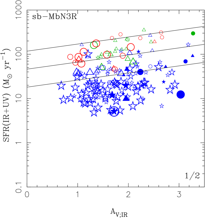
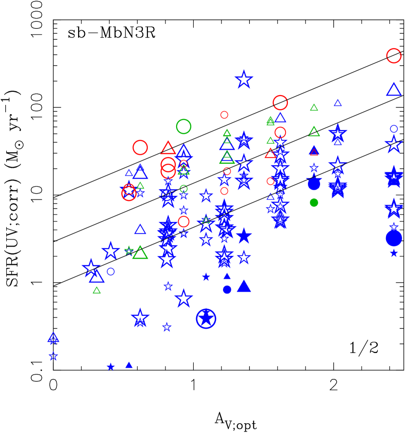
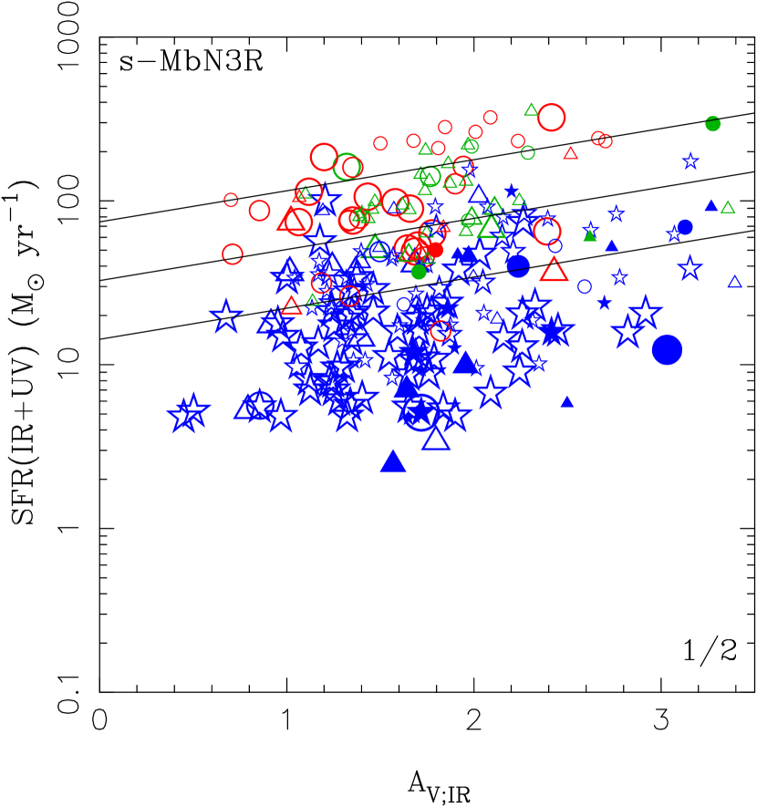
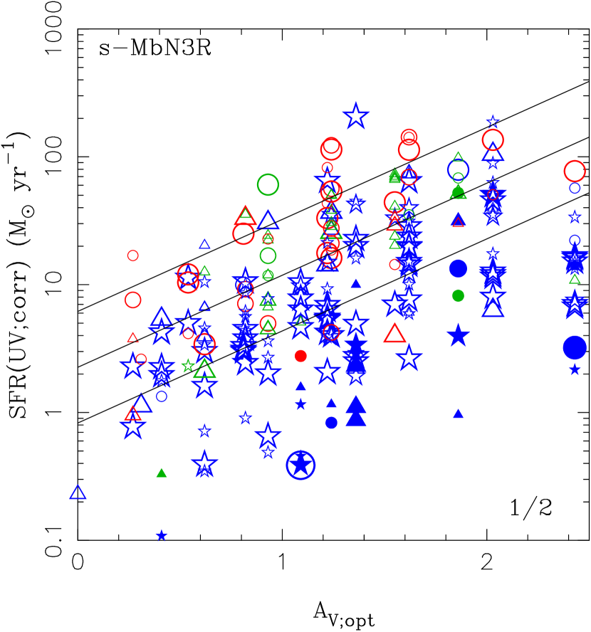
Figure 22: Relation between visual extinction $A_{V}$ and $SFR$ for the s-MbN3Rs and the sb-MbN3Rs. Symbols are the same as in figure 18. Solid lines represent the fitted results with equation (22) for $M_{\ast}=10^{11}M_{\odot}$ at $z=1.5,1.0$, and $0.6$ from top to bottom. Top-Left: For $A_{V;IR}$ and $SFR_{IR+UV}$ of sb-MbN3Rs. Top-Right: For $A_{V;opt}$ and $SFR_{UV:corr}$ of sb-MbN3Rs. Bottom-Left: The same as the Top-Left for s-MbN3Rs. Bottom-Right: The same as the Top-Right for s-MbN3Rs.

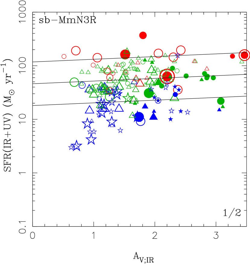
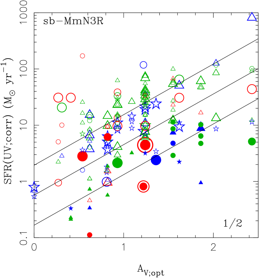
Figure 23: The same as figure 22 for sb-MmN3Rs. Left: For $A_{V;IR}$ and $SFR_{IR+UV}$. Right: For $A_{V;opt}$ and $SFR_{UV:corr}$.

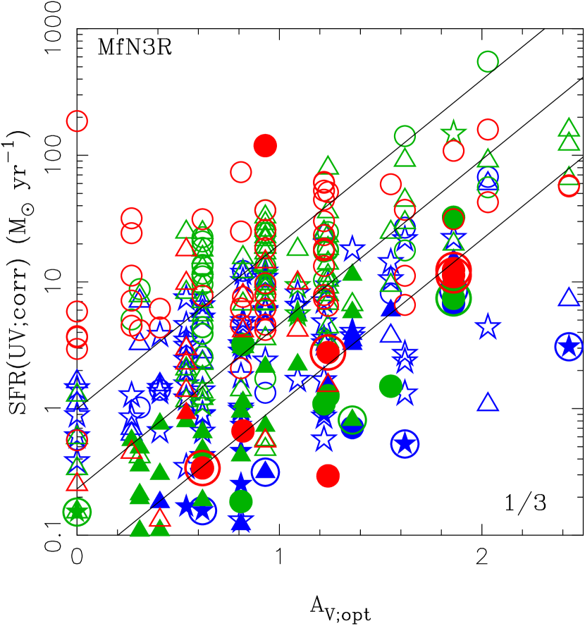
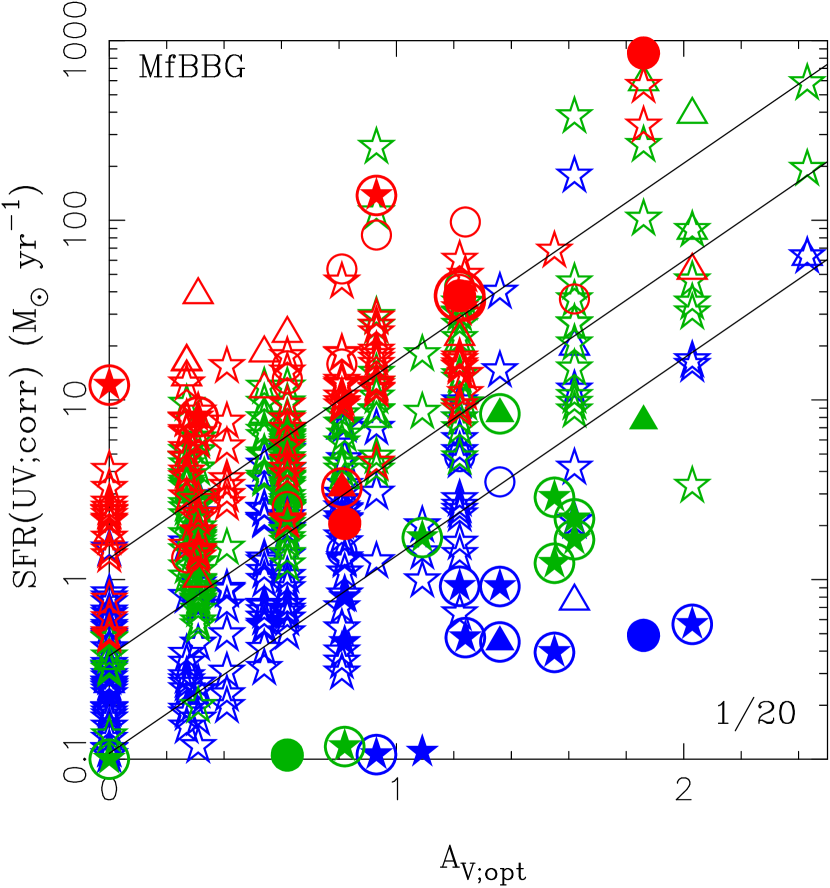
Figure 24: Relation between visual extinction $A_{V}$ and $SFR_{UV:corr}$ for the MfN3Rs and the MfBBGs. Solid lines represent the fitted results with equation (22) for $M_{\ast}=10^{10}M_{\odot}$ at $z=1.5,1.0$, and $0.6$ from top to bottom. Left: For the MfN3Rs. Right: For the MfBBGs.

Table 5: Fitting results with equation (22).

	$\log(\frac{SFR_{0}}{M_{\odot}\mbox{yr}^{-1}})$	$\alpha$	$\beta$	$\gamma$
$A_{V;IR}$
sb-MbN3R	$0.4$	$0.16$	$4.2$	$0.17$
	$\pm 0.1$	$\pm 0.02$	$\pm 0.2$	$\pm 0.04$
s-MbN3R	$0.4$	$0.19$	$3.7$	$0.13$
	$\pm 0.1$	$\pm 0.02$	$\pm 0.2$	$\pm 0.04$
sb-MmN3R	$0.4$	$0.05$	$4.2$	$0.16$
	$\pm 0.1$	$\pm 0.02$	$\pm 0.2$	$\pm 0.03$
$A_{V;opt}$
sb-MbN3R	$-1.1$	$0.67$	$5.2$	$-0.19$
	$\pm 0.2$	$\pm 0.05$	$\pm 0.5$	$\pm 0.08$
s-MbN3R	$-1.0$	$0.72$	$4.5$	$-0.21$
	$\pm 0.1$	$\pm 0.04$	$\pm 0.4$	$\pm 0.06$
sb-MmN3R	$-1.9$	$0.9$	$5.5$	$-0.42$
	$\pm 0.3$	$\pm 0.1$	$\pm 0.8$	$\pm 0.11$
MfN3Rs	$-3.3$	$1.3$	$6.5$	$-0.71$
	$\pm 0.2$	$\pm 0.1$	$\pm 0.4$	$\pm 0.06$
MfBBGs	$-2.3$	$1.1$	$5.6$	$-0.19$
	$\pm 0.2$	$\pm 0.1$	$\pm 0.1$	$\pm 0.06$
Values are means $\pm$ standard deviations.

8.1 Correlation among SFR, extinction, redshift, and mass

Figures 22,  23, and 24 show the correlation between $A_{V}$ and SFR for s-MbN3Rs, sb-MmN3Rs, MfN3Rs, and MfBBGs. For all the subsamples, we have fitted correlations among $A_{V}$, SFR, $z$ and $M_{\ast}$ with a form:

$$\frac{SFR}{SFR_{0}}=10^{\alpha A_{V}}(1+z)^{\beta}\left(\frac{M_{\ast}}{10^{11}M_{\odot}}\right)^{\gamma}\;,$$ (22)

where ${SFR_{0}}$ is a normalization parameter for the SFR in the unit of $M_{\odot}\mbox{yr}^{-1}$. Their best-fitting planes are determined in the space of $A_{V}$, $\log(1+z)$, $\log M_{\ast}$, and $\log SFR$ as summarized in table 5 and shown in figures 22,  23, and 24. For the s-MbN3Rs, we can estimate both classical visual extinction $A_{V}$ with the SED fitting and calorimetric visual extinction $A_{V;IR}$ converted from the calorimetric UV extinction $A_{UV;IR}$ with equation (19) for the best-fitted reddening curve in the optical-NIR SED fitting.

We should remember that $SFR_{IR+UV}$ and $A_{V;IR}$ are estimated from their MIR SED fittings while $SFR_{UV;corr}$ and $A_{V;opt}$ are from their optical SED fittings. This denotes that the trends of $SFR_{IR+UV}$ and $A_{V;IR}$ are independent of those of $SFR_{UV;corr}$ and $A_{V;opt}$. As shown in figure 22, however, the correlation between $SFR_{IR+UV}$ and $A_{V;IR}$ is similar to that between $SFR_{UV;corr}$ and $A_{V;opt}$. Furthermore, the trends, among $SFR_{UV;corr}$, $A_{V;opt}$ and $z_{photz}$, except $M_{\ast}$, are similar to each other not only in the MbN3Rs and the MmN3Rs but also in all the subsamples including the MfN3Rs and MfBBGs as shown in figure 22 (see also table 5). All of them show the same trends; 1) larger SFR, larger extinction $A_{V}$, and 2) lower redshift, larger extinction $A_{V}$. The second trend, increasing $A_{V}$ with the cosmic time, suggests that increasing dust has been induced with chemical enrichment in evolving galaxies.

8.2 Mass dependence and evolution of SFR

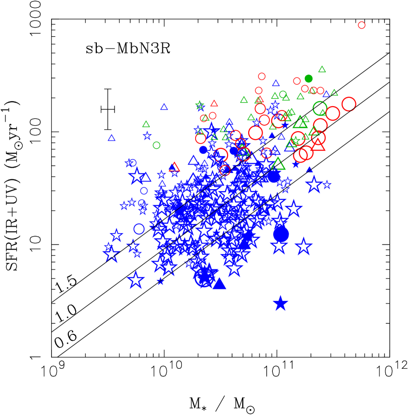
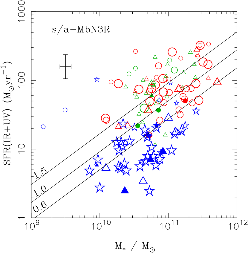
Figure 25: Stellar mass M_∗ vs. $SFR_{IR+UV}$ derived with the TIR and observed UV luminosities. The lines are the same as in figure 27 (see the text in detail). Symbols are the same as in figure 18. Left: For the sb-MbN3Rs. Right: The same as on the left for the star-forming components in the s/a-MbN3Rs.

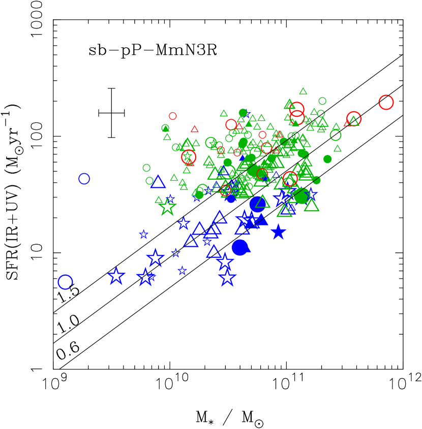
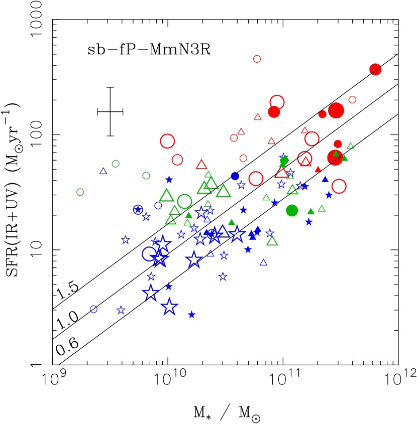
Figure 26: The same as figure 25 for the sb-MmN3Rs. Left: For the sb-pP-MmN3Rs. Right: For the sb-fP-MmN3Rs.

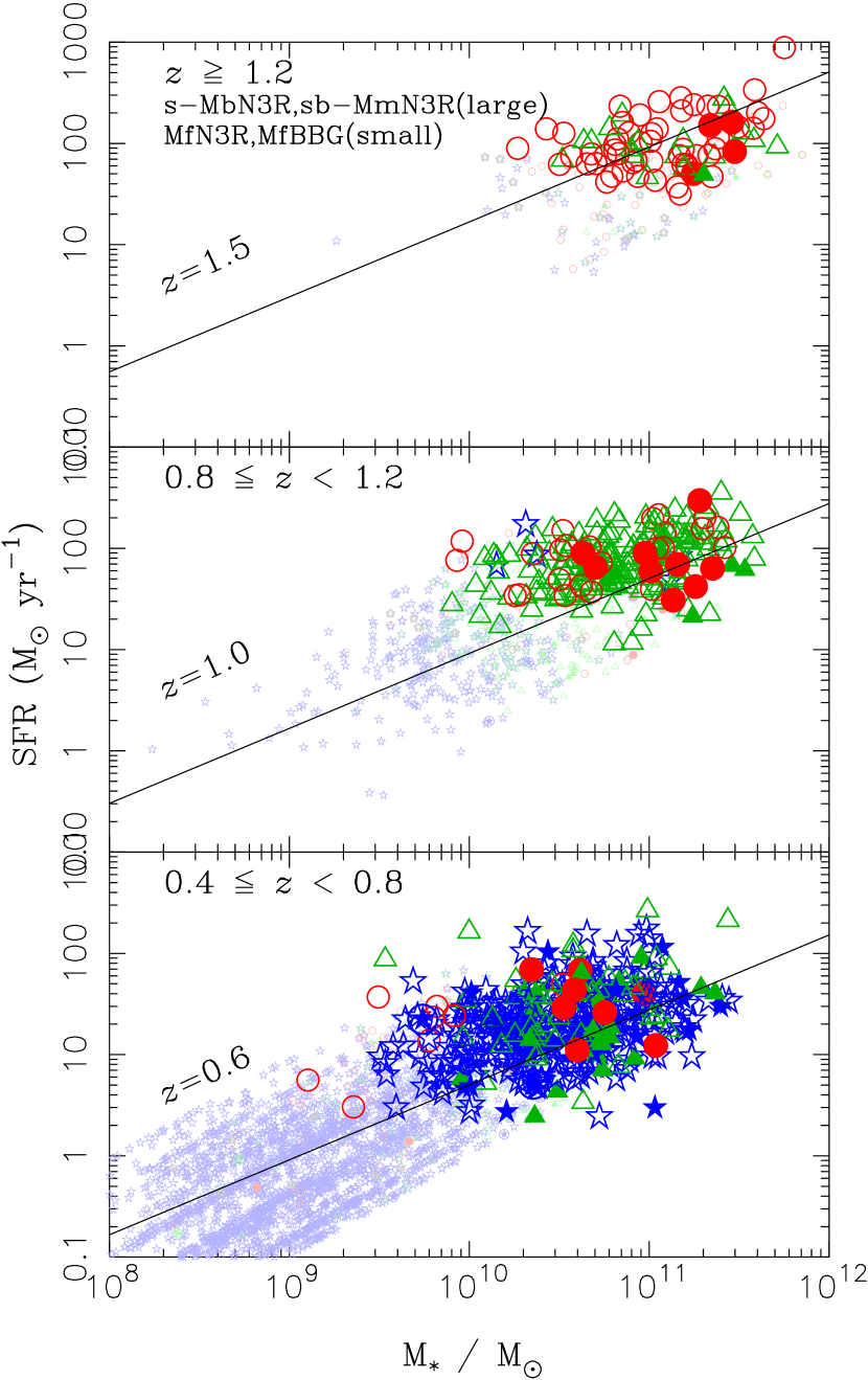
Figure 27: Stellar mass M_∗ vs. SFR for all the star-forming galaxies; the sb-MmN3Rs, MfN3Rs, and MfBBGs. The lines represent the fitting result (see the text in detail). Symbols are the same as in figure 6, except for the large dark and small thin ones represent the MIR-detected star-forming N3Rs (s-MbN3Rs and sb-MmN3Rs) and the MIR faint star-forming galaxies (star-forming MfN3Rs and MfBBGs), respectively. Top: For $z\geqq 1.2$. Middle: For $0.8\leq z<1.2$ Bottom: For $0.4\leq z<0.8$.

Figures 25 and 26 show $SFR_{IR+UV}$ to $M_{\ast}$ for the sb- and s/a-MbN3Rs and sb-MmN3Rs. We can see correlations between $SFR_{IR+UV}$ and $M_{\ast}$, which are more obvious for the sb-MbN3Rs than for the s/a-MbN3Rs. The correlation between $SFR_{IR+UV}$ and $M_{\ast}$ in the sb-MbN3Rs has also an evolutionary trend. The $SFR_{IR+UV}$-$M_{\ast}$ correlation in the s/a-MbN3Rs is more scattered to the lower SFR side from that in the sb-MbN3Rs, in which the decrement becomes more obvious in lower redshifts $z<0.8$ even though the highest mass group around $10^{11}$M_⊙ at higher redshifts $z\geq 0.8$ tends to mostly follow that in the sb-MbN3Rs. They indicate that star formation activities in the s/a-MbN3Rs were quenched at $z<0.8$ compared with those in the sb-MbN3Rs. The indicated connection between quenching star formation and AGN activity around $z\simeq 0.8$ will be discussed with the evolution of the stellar populations in section 9.

The evolutionary trend and mass dependence on the SFR can be seen more clearly in figure 27, for all the star-forming galaxies including the s-MbN3Rs, the sb-MmN3Rs, the star-forming MfN3Rs and the MfBBGs, which are plotted from the top to the bottom in redshift intervals of $0.4\leq z<0.8,0.8\leq z<1.2$, and $z\geq 1.2$. The star-forming MfN3Rs and MfBBGs are selected as the population in the region of “blue cloud” in the $(U-V)-\Delta_{UV}$ color as remarked in subsection 6.4, which excludes extremely young objects fitted with the BC03 models of age $t<0.1$ Gyr.

The mean $SFR$ for all the star-forming galaxies including both the s-MbN3Rs, sb-MmN3Rs, MfN3Rs, and MfBBGs is presented as an approximate function of $M_{\ast}$ and $z$:

$$SFR\left[M_{\odot}yr^{-1}\right]\simeq SFR_{11}\left(\frac{M_{\ast}}{10^{11}\mbox{M}_{\odot}}\right)^{\alpha}(1+z)^{\beta}\;,$$ (23)

where the best-fitting plane in the space of $\log M_{\ast}$, $\log(1+z)$, and $\log SFR$ is determined as $SFR_{11}/M_{\odot}yr^{-1}=7.8$, $\alpha=0.74\pm 0.01$, and $\beta=2.7\pm 0.1$. In figures 25,  26, and  27, the solid lines at $z=0.65,1.0$, and 1.5 represent the best-fitting result. Roughly taking $\alpha\simeq 1$ and $\beta\simeq 3$ for simplification, the growth time scale of the star-forming galaxies is typically derived as

$$\frac{M_{\ast}}{SFR}\left[\mbox{yr}\right]\simeq 10^{10}(1+z)^{-3}\;,$$ (24)

which means the inverse of the sSFR. These SFR evolutionary properties and mass dependence are consistent with previous work for star-forming galaxies selected with general schemes (Noeske et al. 2007; Santini et al. 2009; Dunne et al. 2009; Pannella et al. 2009).

9 Evolution of stellar populations

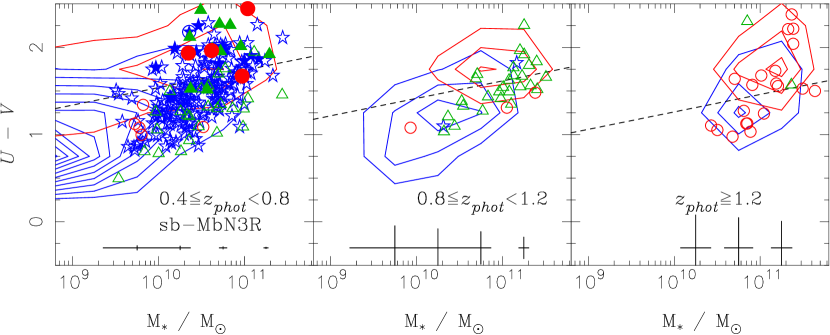
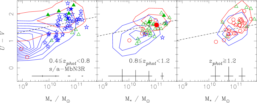
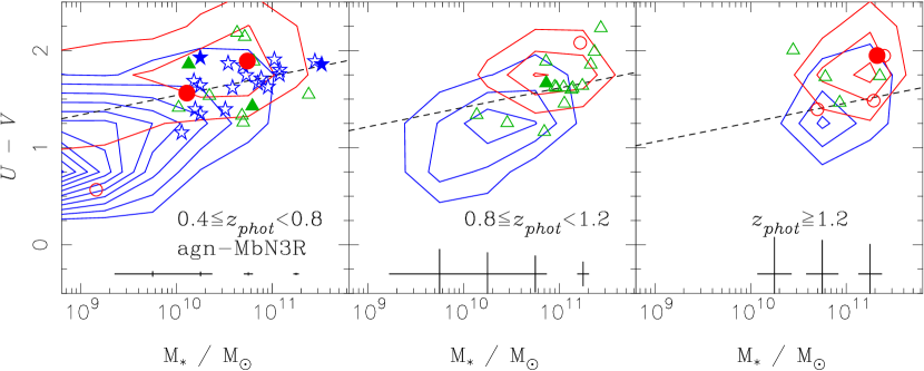
Figure 28: Stellar mass and rest-frame color diagram of $M_{\ast}$ vs. $U-V$ for the MbN3Rs excluded BL AGNs and EBOs. The color is not corrected for dust extinction. Typical errors of the mass and color are represented with crosses at the bottom. Large open and filled symbols and filled symbols in circles represent s-,p-, and qp-BBGs, respectively, which are the same as in figure 6. The plots are for $0.4\leq z<0.8$, $0.8\leq z<1.2$, and $z\geqq 1.2$ from left to right. Red and blue contours represent the rest-frame $V$ detected galaxies with $sSFR<0.1\mbox{Gyr}^{-1}$ and $sSFR>0.1\mbox{Gyr}^{-1}$, respectively. The dotted line corresponds to Bell’s critical line dividing the photometric samples into the blue cloud and the red sequence. Top: Large colored and small gray symbols represent the sb-MbN3Rs and the $z^{\prime}$-detected galaxies, respectively. Middle: The same as the Top for the s/a-MbN3Rs. Bottom: The same as the Top for the agn-MbN3Rs.

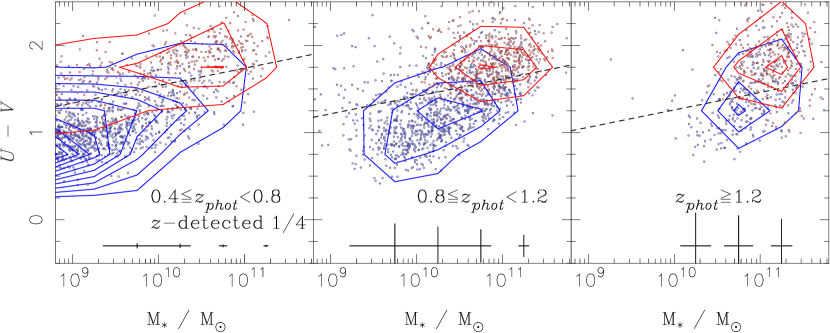
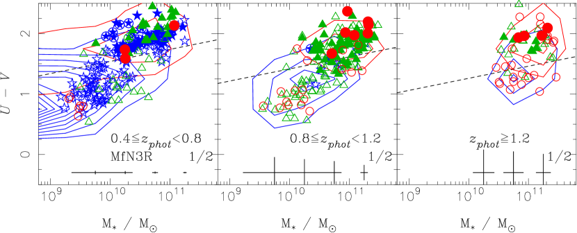
Figure 29: The same as figure 28 for the the rest-frame $V$ detected galaxies and the MfN3Rs. The red and blue small dots with contour represent the rest-frame $V$ detected galaxies with $sSFR<0.1\mbox{Gyr}^{-1}$ and $sSFR>0.1\mbox{Gyr}^{-1}$, respectively. Top: For the rest-frame $V$ detected galaxies. Bottom: For the MfN3Rs.

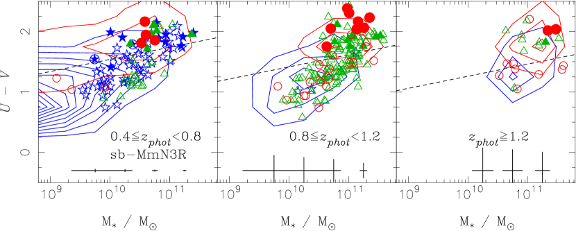
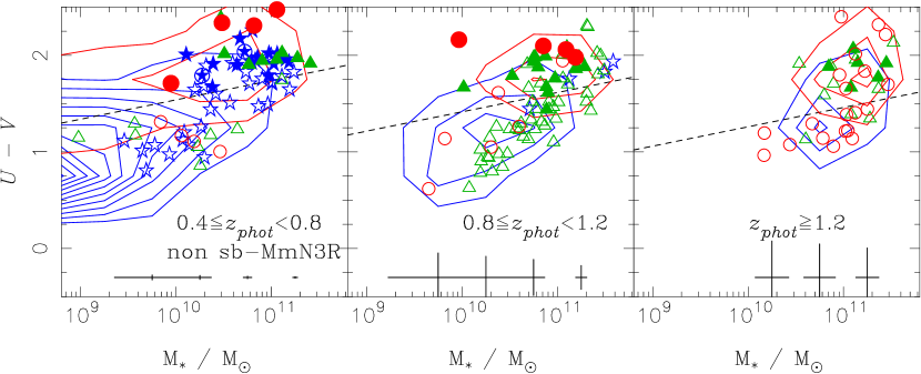
Figure 30: The same as figure 28 for the MmN3Rs. Top: Large colored symbols represent the sb-MmN3Rs. Bottom: The same as the Top for the nsb-MmN3Rs.

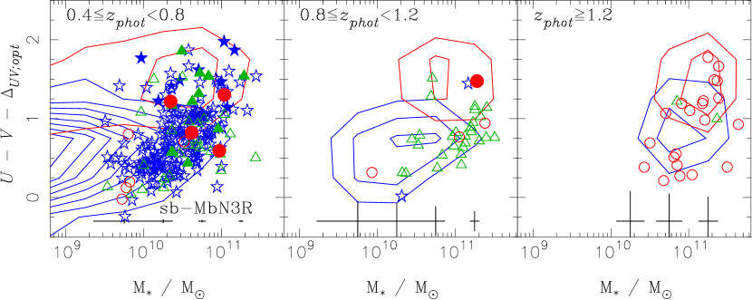
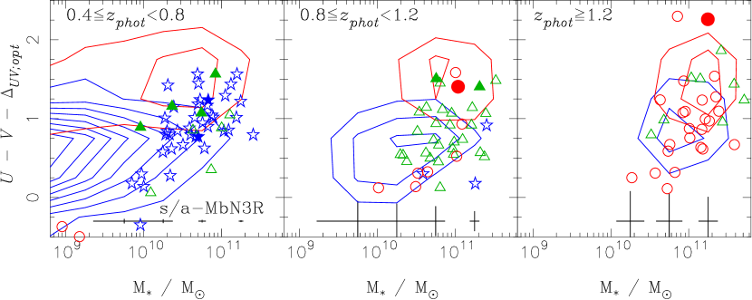
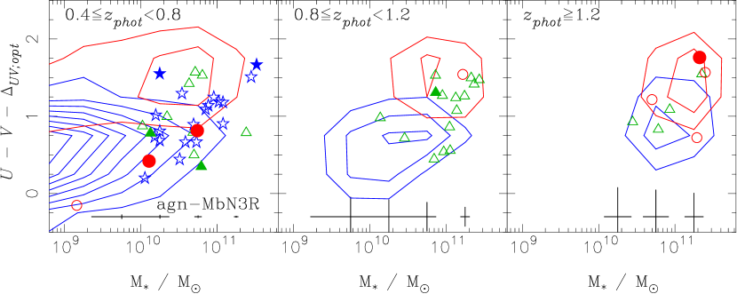
Figure 31: The same as figure 28 for color $U-V-\Delta_{UV}$ corrected using the extinction $A_{UV;opt}$, which is derived from the optical-NIR SED fitting. The sb-,s/a-, and agn-MbN3Rs are plotted from the top to the bottom.

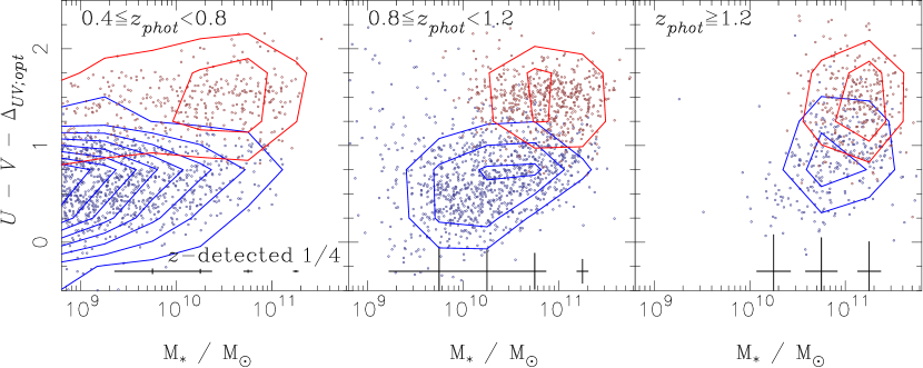
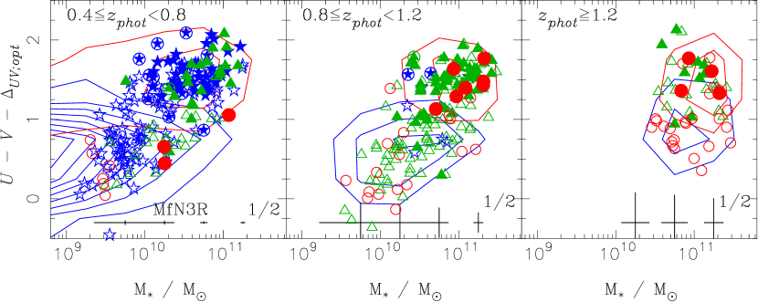
Figure 32: The same as figure 29 for color $U-V-\Delta_{UV}$ corrected using the extinction $A_{UV;opt}$.

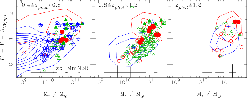
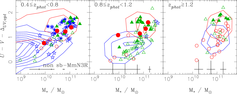
Figure 33: The same as figure 30 for color $U-V-\Delta_{UV}$ corrected using the extinction $A_{UV;opt}$.

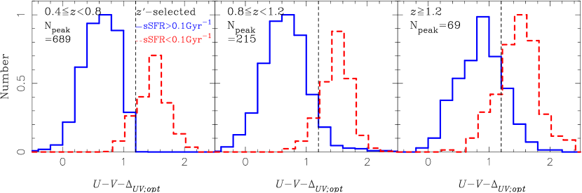
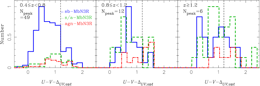
Figure 34: Histograms of the corrected color distribution with $A_{V}$ derived from optical SED fittings. Height of histograms is normalized with the maximum number, which is displayed on the upper-left side. Top: For the rest-frame $V$ detected galaxies, which are classified into two groups with sSFR larger and less than $0.1\mbox{Gyr}^{-1}$, which corresponds to a color $U-V-\Delta=1.2$. Bottom: For the sb-,s/a-, and agn-MbN3Rs.

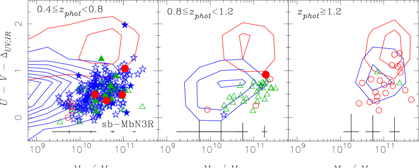
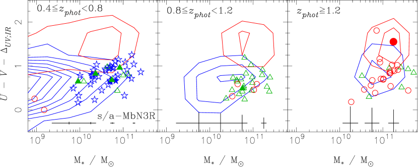
Figure 35: The same as figure 31 for color $U-V-\Delta_{UV}$ corrected using the extinction $A_{UV;IR}$, which is derived with equation (20). Top: For the sb-MbN3Rs. Bottom: For the s/a-MbN3Rs, its remaining dusty starburst component can be extracted and then used to derive $SFR_{IR+UV}$ by fitting its MIR SED with the S&K models.

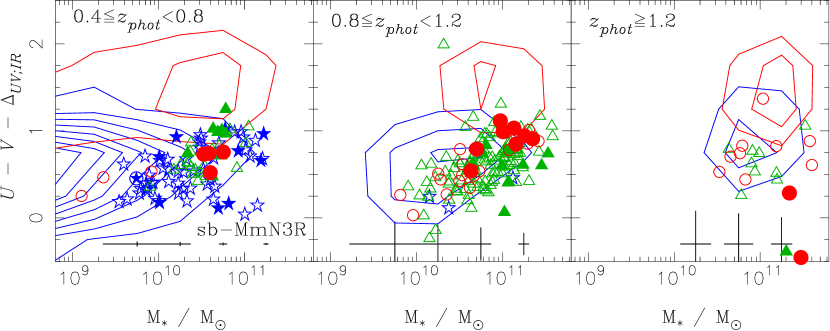
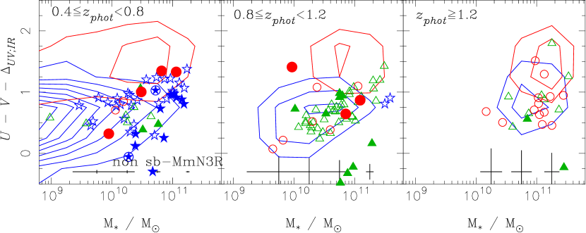
Figure 36: The same as figure 35 for the MmN3Rs. Top: For the sb-MmN3Rs. Bottom: For the non sb-MmN3Rs.

9.1 Rest-frame optical color distributions

The CMD is a powerful tool for studying galaxy evolution since it shows the bimodal galaxy distribution as early types that concentrate in a tight red sequence while late types distribute in a blue dispersed cloud, which have been studied not only in the local Universe with the SDSS (Blanton et al. 2003) but also in the distant Universe with the surveys for $z<1$ (Bell et al. 2004; Faber et al. 2007; Borch et al. 2006) and for $z>1$ (Pannella et al. 2009; Brammer et al. 2009). Spitzer results have also shown that rest-frame colors of MIPS-detected objects, which may overlap with the MbN3Rs and the MmN3Rs, fall between the red sequence and the blue cloud up to $z=2$ (Cowie & Barger 2008; Salim et al. 2009; Brammer et al. 2009).

Thus, we also study rest-frame $U-V$ colors for MbN3Rs and MmN3Rs in the field from their magnitudes interpolated with equation (4). Figure 28 shows the $U-V$ color without extinction correction for the stellar mass $M_{\ast}$ for the sb-, s/a-, and agn-MbN3Rs from top to bottom, where the left, middle, and right figures correspond to the redshift intervals of $0.4\leq z<0.8$, $0.8\leq z<1.2$, and $z\geq 1.2$, respectively, and overplotted contours represent the rest-frame $V$ detected galaxies, which are also shown with the MfN3Rs in figure 29.

The well-known “red and dead” population in a red sequence has a typical color of $U-V\simeq 2$, which can be the reddest ones even in the local Universe with low $A_{V}$ values. However, redder populations of $U-V>2$ can clearly be seen in all the diagrams not only for the MbN3Rs but also for the MmN3Rs and even for the MfN3Rs as shown in figures 28,  30 and  29. It suggests that not only the MbN3Rs but also the MmN3Rs and most of the MfN3Rs suffer from dust extinction, which is already expected from the results in section 8. Thus, we have taken into account color corrections for these diagrams. Figures 31,  32, and  33 represent intrinsic stellar color $(U-V)-\Delta_{UV}$ corrected for extinction using $A_{UV;opt}$ derived from the optical-NIR SED fitting. In the top diagram of figure 31, we can see that the bimodal color distribution of the MbN3Rs persists even up to $z\simeq 1.2$, which is also consistent with the BBG classification as p-BBGs mainly appear in the region of a red sequence. As discussed in appendix A.3, unfortunately, our $K_{s}$ photometry is not deep enough to obtain a complete sample up to $z\geq 1.2$, which may be one of the reasons why the bimodal feature at $z\geq 1.2$ is not so clear compared with the results of Brammer et al. (2009).

Figure 35 also shows the intrinsic colors of stellar components in the sb- and s/a-MbN3Rs, in which the colors are corrected with $A_{UV;IR}$. Few of them remain in the red sequence region, which comes from the effect of the extinctions as discussed in subsection 7.3: $\langle A_{UV;IR}\rangle\simeq\langle A_{UV;opt}\rangle+\langle\Delta A_{UV}\rangle$ with $\langle\Delta A_{UV}\rangle\sim 0.5$ as long as $f_{SK}=1$. Furthermore, we cannot clearly see the bimodality in figure 35 compared with figure 31. The same trends can be also confirmed for the MmN3Rs as shown in figures 31 and  36. Even if we have $\langle\Delta A_{UV}\rangle\sim 0$ by taking the proportional factor as $f_{sk}\simeq 0.3$, we just obtain a bluer mean color by adding $\simeq 0.5$ without recovering the bimodality. It suggests that it is appropriate to correct the color of a whole galaxy in the classical way with $A_{UV;opt}$ even for dusty systems as the MbN3Rs and the MmN3Rs. Thus, we will discuss the evolution of stellar populations along with the results corrected with $A_{UV;opt}$ as figure 31 in the following.

We can see the evolutionary trends for sb-, s/a-, and agn-MbN3Rs in figures 31 and 34 and will summarize as follows. In all redshifts, the sb-MbN3Rs mainly stay in the area $U-V-\Delta<1$. It can be interpreted as they are on-going in star formation. On the other hand, the agn-MbN3Rs start to appear even around $U-V-\Delta<1$ at $z\geq 1.2$ with large scatters in a mass range $>3\times 10^{10}M_{\odot}$, and relatively concentrate around $U-V-\Delta\sim 1$ at $0.8\leq z<1.2$ as shown in the bottom diagrams of figure 31. The trend, as starbursts are bluer than AGNs at $0.8\leq z<1.2$, can be seen not only for the MbN3Rs but also for the MmN3Rs in figure  33. Figures 31 and 33 also show that the sb-MmN3Rs are relatively redder than the sb-MbN3Rs in the same stellar mass. It is reasonable as the former with less luminous IR emissions may have smaller SFRs and quench their SF activities more effectively than the latter.

As shown in the middle of figure 31, the s/a-MbN3Rs have a similar stellar population of the sb-MbN3Rs at $z\geq 0.8$ even though some of them were $U-V-\Delta>1$. Thus, a dusty star formation cannot suffer from the obscured AGN activity at $z\geq 0.8$ at least. On the other hand, at $z<0.8$, it is similar to the agn-MbN3Rs at around $U-V-\Delta\sim 1$. Passive populations such as the p-BBGs and on the red sequence are relatively major in s/a-MbN3Rs at $0.8\leq z<1.2$. This suggests the co-existence of the obscured AGN with passive stellar populations in their hosts, which are older than those in the sb-MbN3Rs. Thus, the stellar populations become already passive in massive galaxies such as the s/a-MbN3Rs of $\simeq 10^{11}$M_⊙ with obscured AGNs even at $z\simeq 1$, and the obscured AGNs are activated in less-massive galaxies of $<10^{11}$M_⊙ mainly with star formation at $z<0.8$. These indications from the CMDs are consistent with the indication about quenching SFRs of the s/a-MbN3Rs at $z<0.8$ from figures 25 and 26. It suggests that the evolution of AGN activity is more rapid than that of star-formation around $z=1-2$ and that the co-evolutionary link between AGN activity and star formation in galaxies can be critical around $z\simeq 1$. This seems to remind us of a scenario where AGN activity may quench the star formation in the distant universe to explain the downsizing.

10 Evolution of AGN activities

10.1 AGN activity traced at rest-frame 5 $\mu$m

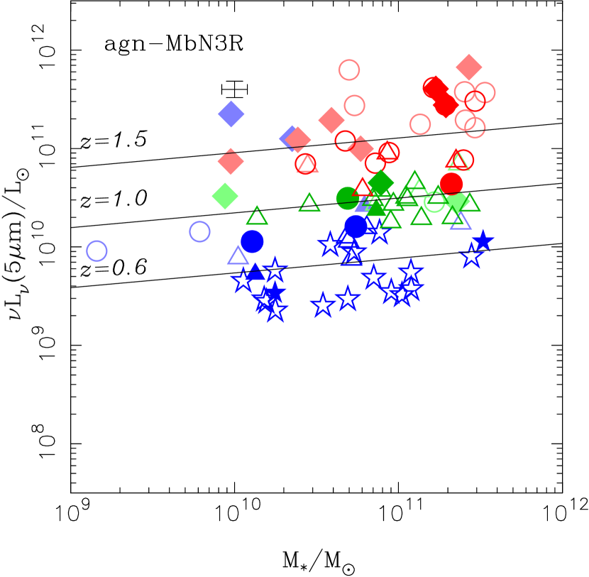
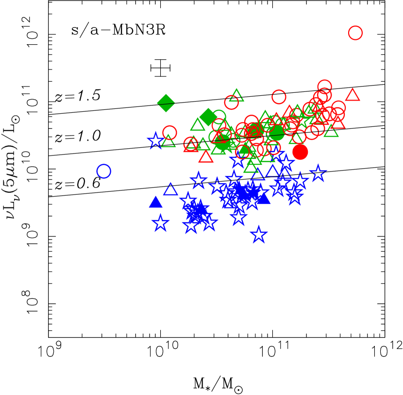
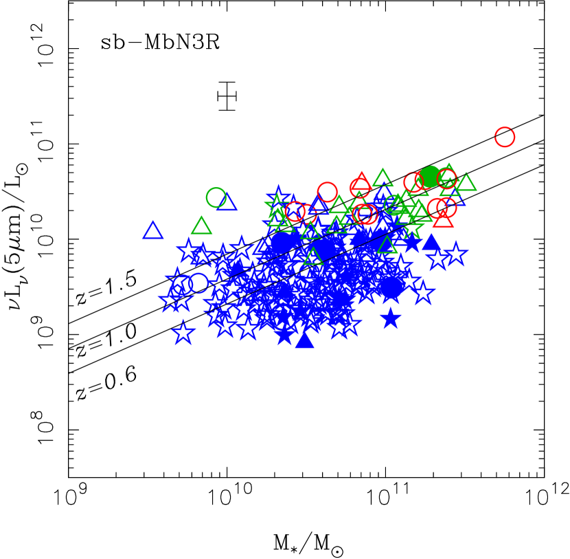
Figure 37: Correlation between stellar mass $M_{\ast}$ vs. $\nu L_{\nu}(5~{}\mu\mbox{m})$ at rest-frame 5 $\mu$m for the MbN3Rs. Symbols represent the same as in figure 6 except for the colors. The blue, green, and red symbols represent objects at the redshifts of $0.4\leq z<0.8$, $0.8\leq z<1.2$, and $z\geq 1.2$, respectively. Diamonds represent the spectroscopic BL AGNs. Dark and faint symbols represent objects with reduced $\chi^{2}<0.5$ and $\chi^{2}>0.5$ in the MIR SED fitting, respectively. Top: For the agn-MbN3Rs. Bottom-Left: For the s/a-MbN3Rs. Bottom-Right: For the sb-MbN3Rs.

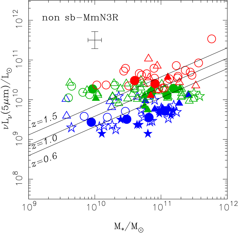
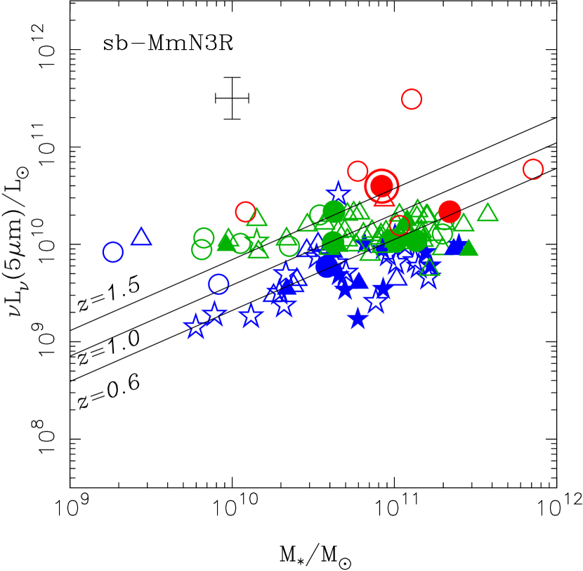
Figure 38: The same as figure 37 for the MmN3Rs. Left: For the non sb-MmN3Rs. Right: For the sb-MmN3Rs.

Figure 37 shows the rest-frame absolute monochromatic luminosities $\nu L_{\nu;5}$ at 5 $\mu$m to their stellar mass $M_{\ast}$ derived with equation (4), for the agn-MbN3Rs, the sb-MbN3Rs and the s/a-MbN3Rs. We can see an evolutionary trend as the agn-MbN3Rs at higher redshifts are more luminous at 5 $\mu$m. The mass and evolutionary trend for $\nu L_{\nu;5}$ is roughly summarized as:

$$\nu L_{\nu;5}\left[L_{\odot}\right]\simeq L_{11}\left(\frac{M_{\ast}}{10^{11}M_{\odot}}\right)^{\alpha}(1+z)^{\beta}\;,$$ (25)

In figure 37, the data points of the MbN3Rs are plotted in redshift intervals of $0.4\leq z<0.8,0.8\leq z<1.2,1.2\leq z$, respectively. The solid line for agn- and s/a-MbN3Rs at $z=0.6,1.0$, and 1.5 represents the best-fitted plane of $\log(L_{11}/L_{\odot})=8.9\pm 0.1$, $\alpha=0.15\pm 0.08$, and $\beta=6.3\pm 0.4$ in equation (25). On the other hand, the solid lines for sb-MbN3Rs represent the plane of $\alpha=0.74$ and $\beta=2.7$, which are the same expornents of equation (23) for star-forming activities in subsection 7.1. Thus, the 5-$\mu$m emissions of the sb-MbN3Rs are dominant from their dusty star-forming regions.

The trends for the 5-$\mu$m luminosities do not depend on their selections since the $\nu L_{\nu;5}$ of the MbN3Rs is larger than the limiting luminosities for their detection as $\simeq 10^{9},6\times 10^{9}$, and $2\times 10^{10}L_{\odot}$ at $z=0.5,1.0$, and 1.5, respectively. Thus, the emission process at the rest-frame 5 $\mu$m for the agn- and the s/a-MbN3Rs should be different from the dusty star-forming origin for the sb-MbN3Rs. This supports the supposition that MIR emissions from the agn-MbN3Rs are dominated by obscured AGN. Thus, it is expected that the 5-$\mu$m luminosity $\nu L_{\nu;5}$ may dominate in the bolometric luminosity of the obscured AGN $L_{bol}$ for the s/a- and agn-MbN3Rs.

The evolutionary trend of $\nu L_{\nu;5}$ in the agn-MbN3Rs is more rapid than that of SFRs in the sb-MbN3Rs. The $\nu L_{\nu;5}$ in the agn-MbN3Rs at $0.8\leq z<1.2$ and $0.4\leq z<0.8$ also becomes less scattered than those at $z\geq 1.2$, which can be attributable to quenching the AGN activities around $z\simeq 1$.

The analysis with $\nu L_{\nu;5}$ can also apply for the MmN3Rs as shown in figure 38 even though they are biased since most of them are detected in critical threshold at the rest-frame 5 $\mu$m. The sb-MmN3Rs and the non sb-MmN3Rs show roughly a similar trend to those of the sb-MbN3Rs and the s/a-MbN3Rs compared with the agn-MbN3Rs, which suggests that AGN activities are not dominant in the MmN3Rs.

10.2 Super Massive Black Holes in AGNs

Consider accretion onto the Super Massive Black Hole (SMBH) with a mass $M_{BH}$ for an AGN. The bolometric luminosity $L_{bol}$ of the emission from the AGN is characterized by an Eddington ratio $\lambda$ as $L_{bol}=\lambda L_{Edd}$ and the Eddington luminosity $L_{Edd}$:

$$L_{Edd}\left[erg\;s^{-1}\right]=1.26\times 10^{38}\left(\frac{M_{BH}}{M_{\odot}}\right)\;.$$ (26)

Introducing a luminosity ratio $f_{5}=\nu L_{\nu;5}/L_{bol}$, we can obtain a constraint for the mass of the SMBH from the 5-$\mu$m luminosity $\nu L_{\nu;5}$ as

$$\frac{M_{BH}}{3.06\times 10^{6}M_{\odot}} = \lambda^{-1}f_{5}^{-1}\frac{\nu L_{\nu;5}}{10^{11}L_{\odot}}\;.$$ (27)

We can see $\nu L_{\nu;5}\simeq 10^{12}L_{\odot}$, and $3\times 10^{10}L_{\odot}$ at maximum, and minimum, respectively, for the agn-MbN3Rs of $M_{\ast}\simeq 10^{11}M_{\odot}$ at $z>1.2$ in figure 37. It means that SMBHs had already grown in a mass range of $\simeq 10^{6}\lambda^{-1}f_{5}^{-1}M_{\odot}-3\times 10^{7}\lambda^{-1}f_{5}^{-1}M_{\odot}>10^{6}M_{\odot}$ in a host of $M_{\ast}\simeq 10^{11}M_{\odot}$ selected as the agn-MbN3Rs at $z>1.2$. Furthermore, as long as $\lambda f_{5}>10^{-1}$, the BH mass in a maximum 5-$\mu$m luminous agn-MbN3R of $M_{\ast}\simeq 10^{11}M_{\odot}$ at $z>1.2$ does not exceed $3\times 10^{8}M_{\odot}$, which is a similar value attributable to the relation between the mass of SMBH and the stellar mass in the local spheroid as derived by Häring & Rix (2004):

$$\log{M_{BH}} = -4.12+1.12(\log M_{\ast})\;.$$ (28)

If the mass relation between SMBH and host was already established at $z>1.2$ as this equation (28) in the local Universe, then, the AGN luminosity in the agn-MbN3Rs at $z>1.2$ could be near the Eddington limit $\lambda\simeq 1$, which is consistent with consideration about SMBH growth history as follows.

Introducing an energy conversion efficiency $\epsilon=L_{bol}/(\dot{M}c^{2})$ for mass accretion with $\dot{M}$ onto an SMBH, the 5-$\mu$m luminosity $\nu L_{\nu;5}$ also implies a constraint for a mass growth ratio $\dot{M}_{BH}$ of SMBHs as

$$\frac{\dot{M}_{BH}}{6.8\times 10^{-3}M_{\odot}yr^{-1}}=(1-\epsilon)\epsilon^{-1}f_{5}^{-1}\frac{\nu L_{\nu;5}}{10^{11}L_{\odot}}\;,$$ (29)

where we have used $\dot{M}_{BH}=(1-\epsilon)\dot{M}$ and $\nu L_{\nu;5}=f_{5}L_{bol}$. The thin-disk accretion model has predicted the efficiency $\epsilon$ should be in the range $\simeq 0.04-0.31$, depending on the spin of SMBH. The growth time scale of SMBHs is also represented as

$$\frac{M_{BH}}{\dot{M}_{BH}}\left[\mbox{yr}\right]=4.5\times 10^{8}\lambda^{-1}\frac{\epsilon}{(1-\epsilon)}\;.$$ (30)

Then, the SMBH growth time could be less than the time of $\simeq 2.5$ Gyr from z=2 to z=1 for $\lambda/\epsilon>0.2$, which can be satisfied as long as it is near the Eddington limit with $\lambda>0.06$ for assuming the thin-disk accretion model with $\epsilon=0.04-0.31$. Thus, it is consistent with the suggestion that SMBHs had already grown in the maximum 5-$\mu$m luminous agn-MbN3Rs of $M_{\ast}\simeq 10^{11}M_{\odot}$ at $z>1.2$ and their AGN luminosity could be near the Eddington limit $\lambda\simeq 1$ as discussed above.

10.3 AGN activity and star formation

Even though the sb-MbN3Rs and the agn-MbN3Rs are different populations, we could obtain simple formulae representing the activity of star formation and obscured AGN in the MbN3Rs up to $z\simeq 2$ with functions of their stellar mass and redshift as equations (23) and (25). The 5-$\mu$m luminosity of the agn-MbN3Rs is rapidly quenching as equation (25) compared with that of sb-MbN3Rs as equation (23). It means that the evolutionary time scale of AGN activity is shorter than that of star formation for the MbN3Rs selected with the AKARI MIR photometry.

The rapid evolutionary trend of AGNs in the MbN3Rs was already expected from its color of stellar population as discussed in section 9. Thus, this evolutionary trend in the time scales, which distinguishes between the agn-MbN3Rs and the sb-MbN3Rs, is consistent with the evolutionary feature of the MbN3Rs around $z\simeq 1$ in their distribution on the color-mass diagram as shown in figure 35.

11 Discussions

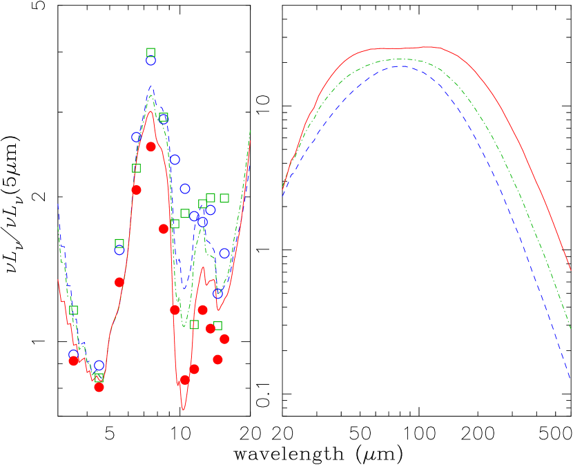
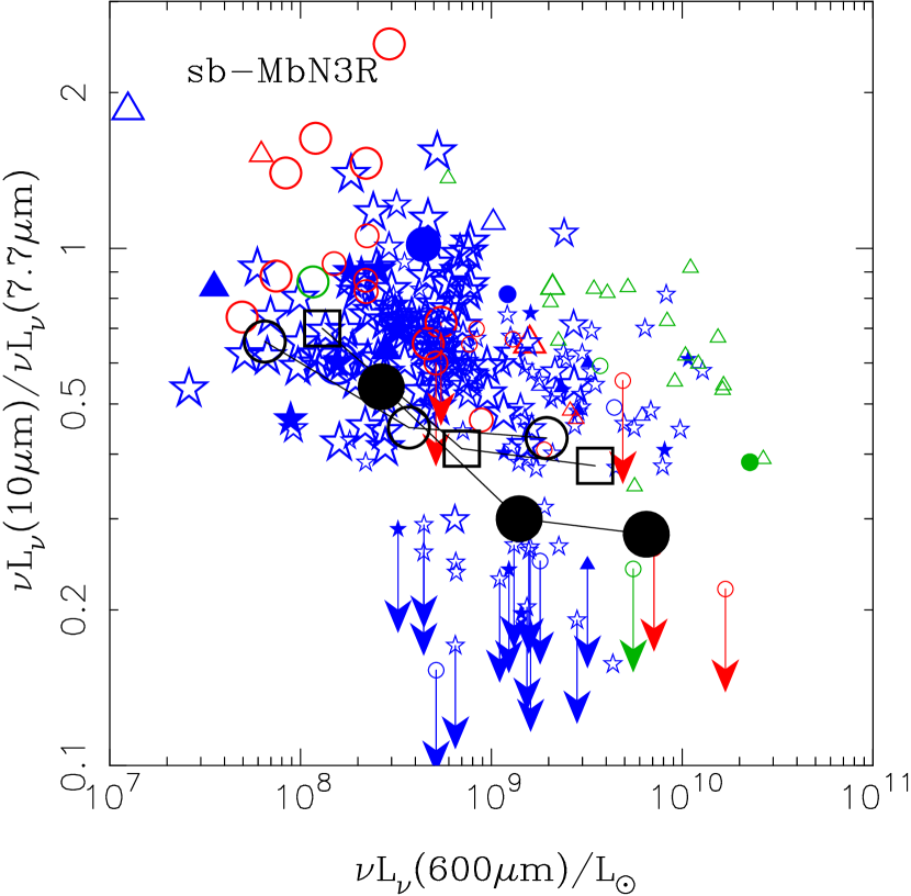
Figure 39: Left: Averaged rest frame IR-Submm SEDs for the sb-MbN3Rs. Red filled circles, green open squares, and blue open circles represent monochromatic luminosity $\nu L_{\nu}$ averaged for the sb-MbN3Rs which fit well with large, medium, and small optical depth S&K models of $A_{V;SK}=17.9,6.7$, and 2.2, respectively. Red solid, green dotted, and blue dashed lines represent model SEDs with $A_{V;SK}=17.9,6.7$, and 2.2, respectively. The model SEDs have been convoluted within a 3 $\mu$m wavelength corresponding to a mean width of the AKARI/IRC bands. Right: Expected monochromatic luminosity at rest-frame $600~{}\mu\mbox{m}$; $\nu L_{\nu}(600~{}\mu\mbox{m})$ vs. monochromatic luminosity ratio at rest-frame $10~{}\mu\mbox{m}$ to $7.7~{}\mu\mbox{m}$; $\nu L_{\nu}(10~{}\mu\mbox{m})/\nu L_{\nu}(7.7~{}\mu\mbox{m})$ for a case with TIR luminosity $L_{IR}=5\times 10^{11}$ L_⊙. Black filled circles, open squares, and open circles represent monochromatic luminosities $\nu L_{\nu}(10~{}\mu\mbox{m})/\nu L_{\nu}(7.7~{}\mu\mbox{m})$ from the convoluted S&K models with $A_{V;SK}=17.9,6.7$, and 2.2, respectively. We have taken other S&K model parameters as $L^{tot}=10^{10.1},10^{11.1},\mbox{and}10^{12.1}$ L_⊙ from right to left and fixed $L_{OB}/L^{tot}=0.6$.

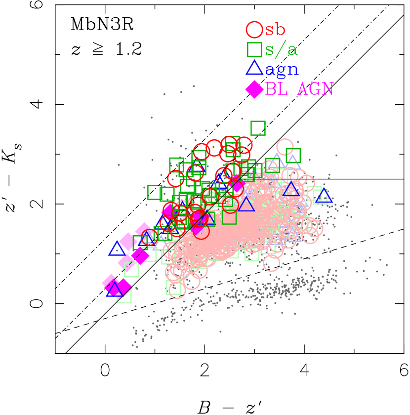
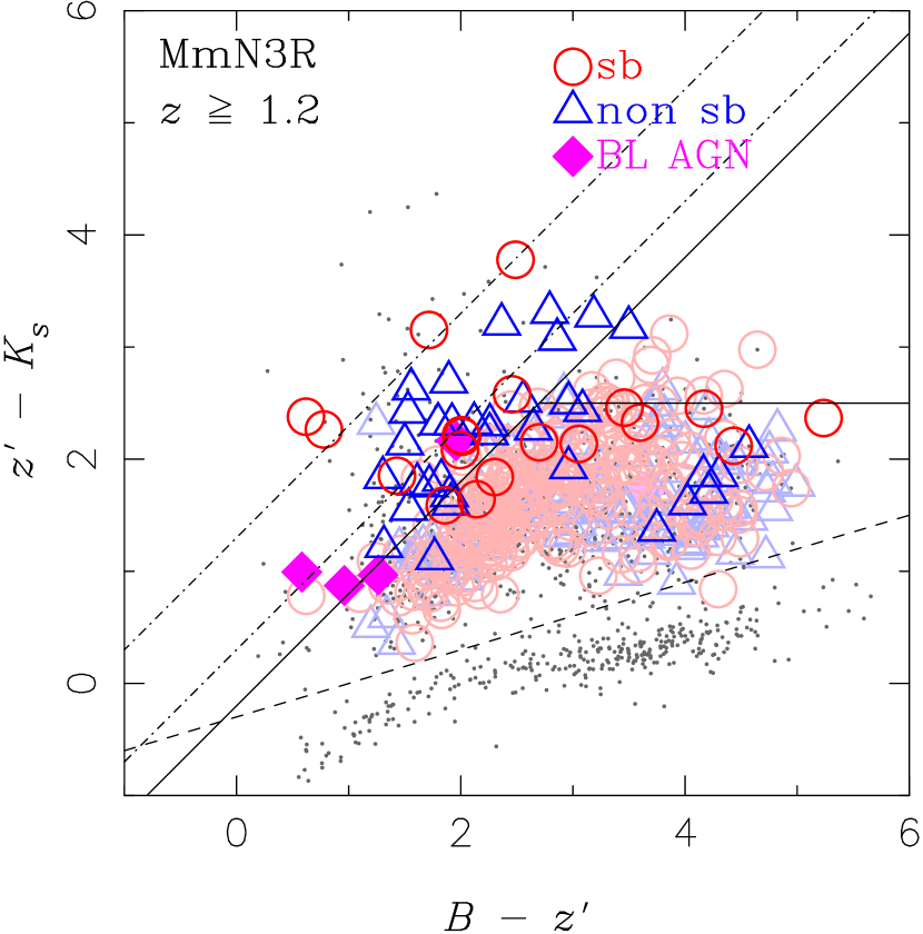
Figure 40: $BzK$ color diagram for the MbN3Rs and MmN3Rs. Large dark and faint symbols represent galaxies at $z\geq 1.2$ and $z<1.2)$, resepectively. The small dots represent the MIR faint galaxies with $K<21$. Left: For the MbN3Rs. Red open circles, green open squares, blue open triangles, and magenta filled diamonds represent sb-, s/a-, agn-MbN3R, and BL-AGN, respectively. Right: For the MmN3Rs. Red open circles, green open squares and magenta filled diamonds represent sb-, non sb-MmN3R, and BL-AGN, respectively.

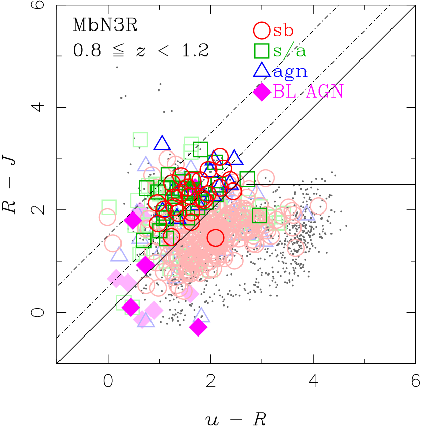
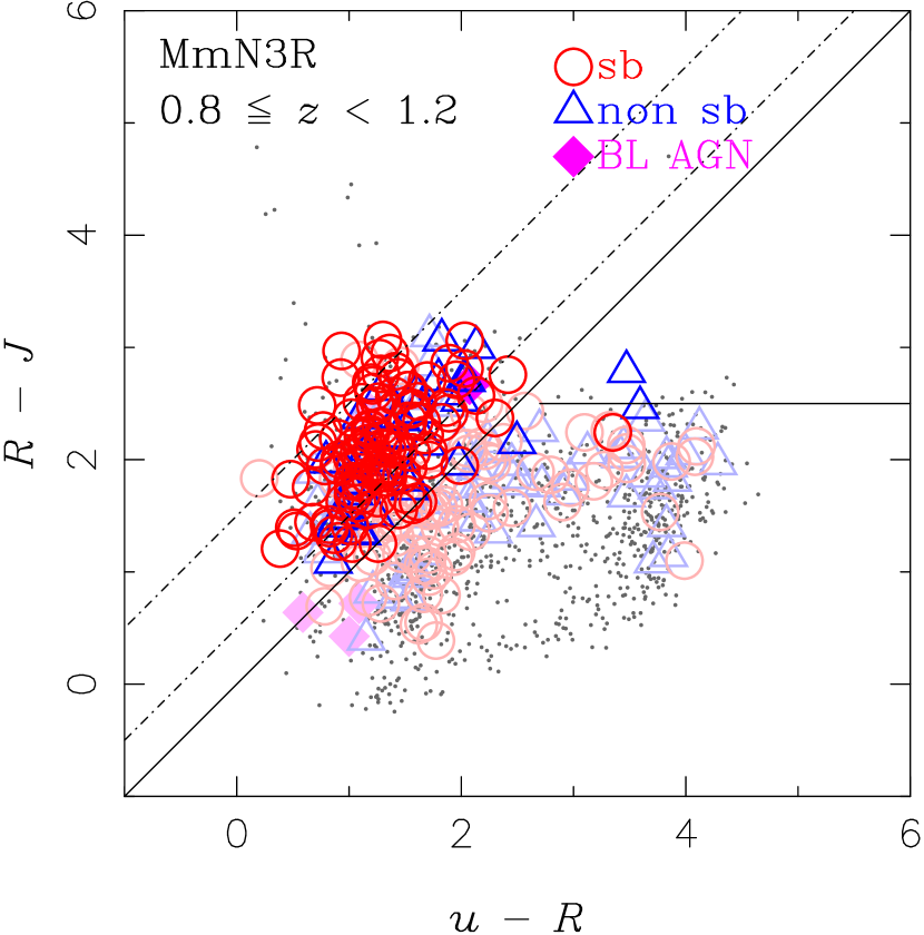
Figure 41: The same as figure 40 for the $uRJ$ color diagram. Large dark and faint symbols represent galaxies at $0.8\leq z<1.2$ and $z<0.8$, respectively. Small dots represents the MIR faint galaxies with $J<22$.

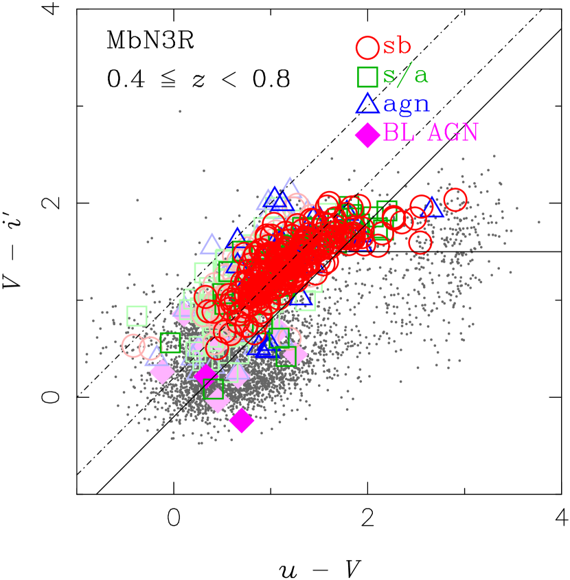
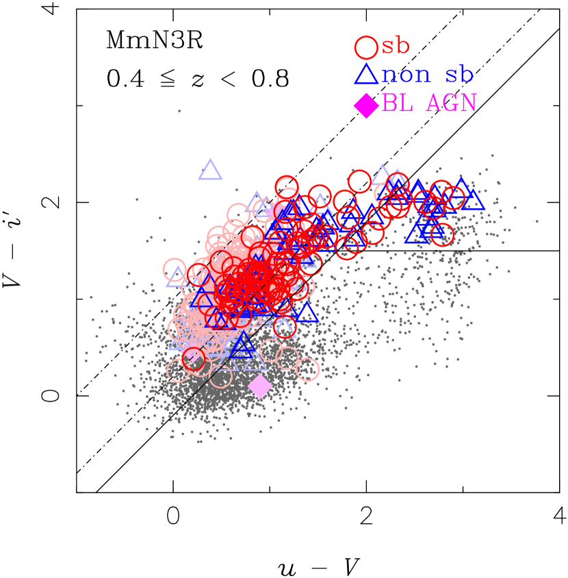
Figure 42: The same as figure 40 for the $uVi$ color diagram.

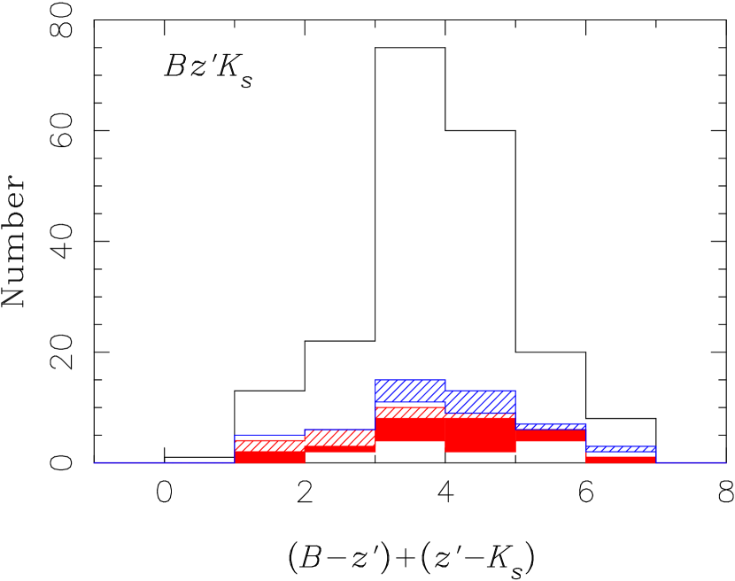
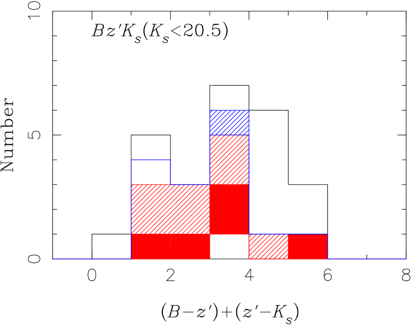
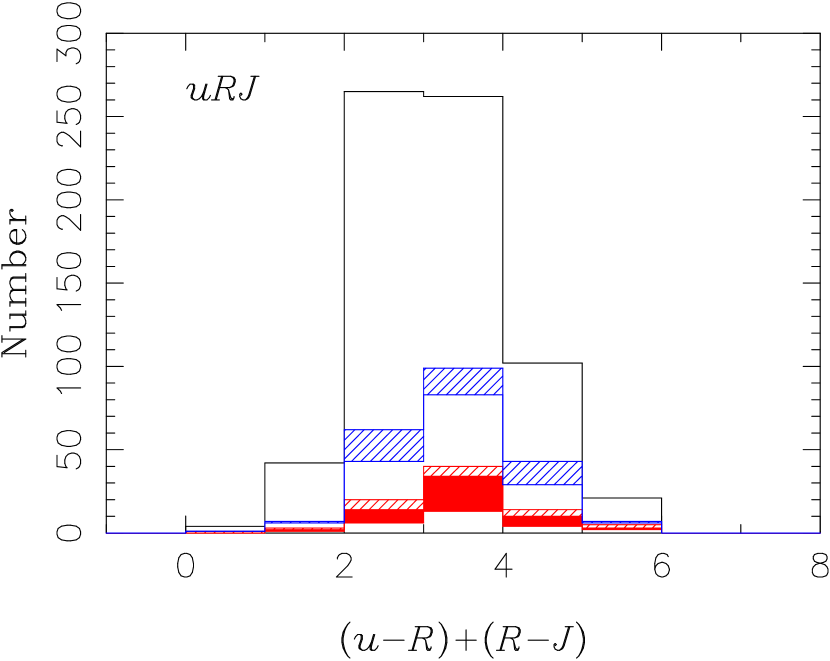
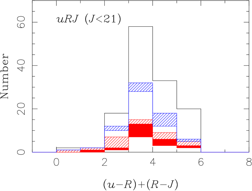
Figure 43: Color distribution of the MbN3Rs along the strip between the dashed lines in figures 40 and  41. Top solid line histogram indicates the number of galaxies detected in the NIR band. Red slashed, filled, and outline histograms represent agn-, s/a-, and sb-MbN3Rs, respectively. Blue slashed and outline histograms represent and non sb-MmN3Rs and sb-MmN3Rs, respectively.

11.1 FIR and Submillimeter Follow-ups

As discussed in subsection 7.3, the s-MbN3Rs and the sb-MmN3Rs with a lower ratio of monochromatic luminosity at rest-frame $10~{}\mu\mbox{m}$ to that at $7.7~{}\mu\mbox{m}$; $\nu L_{\nu}(10~{}\mu\mbox{m})/\nu L_{\nu}(7.7~{}\mu\mbox{m})$ tend to have larger extinctions assuming denser dust distributions (see in figure 21). Larger extinctions, indicated with $\nu L_{\nu}(10~{}\mu\mbox{m})/\nu L_{\nu}(7.7~{}\mu\mbox{m})$, can make reprocessed photon emissions dominant at longer wavelengths. This trend can be confirmed in the left plot of figure 39, which shows the average IR/Submm SEDs for the s-MbN3Rs fitted well with large, medium, and small optical depth parameters in S&K model; $A_{V;SK}=17.9$, 6.7, and 2.2, respectively. The s-MbN3Rs with a larger optical depth tend to show not only a deeper dip at $10~{}\mu$m but also a larger flux in FIR and submillimeter wavelengths. This feature can be confirmed directly with observations with FIR devices such as the Photodetector Array Camera (PACS) and Photometric Imaging Receiver (SPIRE) on board Herschel and submillimeter telescopes as MAMBO/IRAM and ALMA. Figure 39 shows the expected monochromatic luminosity at rest-frame $600~{}\mu\mbox{m}$; $\nu L_{\nu}(600~{}\mu\mbox{m})$ vs. $\nu L_{\nu}(10~{}\mu\mbox{m})/\nu L_{\nu}(7.7~{}\mu\mbox{m})$ as the trend between extinctions and FIR/Submm wavelength excess.

Observations with ground-based submillimeter telescopes as SCUBA and MAMBO have reported that so-called high-z SMGs tend to have SEDs reproduced with lower dust temperatures when compared with local ULIRGs (e.g. Chapman et al. (2004)), which suggests that detection of the SMGs with the ground-based submillimeter telescopes could be biased and there are missing populations of star-forming galaxies with hotter dust as Optically Faint Radio Galaxies (OFRGs). Recently the PACS and SPIRE/Herschel observations have revealed that ULIRGs at $z\simeq 2$ detected with the MIPS/Spitzer consist of both cold and warm populations corresponding to the SMGs and the OFRGs (Magdis et al. (2010); Elbaz et al. 2011), respectively. Even though our samples of MbN3Rs and MmN3Rs may not overlap with the Herschel detected ULIRG samples since our samples were detected in the MIR bands and correspond to LIRGs at $z\simeq 1$, the variety of $\nu L_{\nu}(10~{}\mu\mbox{m})/\nu L_{\nu}(7.7~{}\mu\mbox{m})$ suggests that LIRGs at $z\simeq 1$ may consist of various populations with cold and warm dusts similar to the ULIRGs at $z\simeq 2$ such as the SMGs. The forthcoming and future observations with Herschel and submillimeter telescopes will confirm these features as predicted in figure 39.

Adding these photometric data at these longer wavelengths for the MbN3Rs can also serve as a strong constraint in the SED analysis with direct estimation of their TIR luminosities, which can overcome an ambiguity left in deriving absolute TIR luminosity by introducing the proportional factor $f_{SK}$ in section 7. Furthermore, this makes a distinction between starburst dominant and AGN dominant with the FIR/Submm luminosity with the MIR one, which is an alternative way to determine the MIR color criteria for selecting s- and agn-MbN3Rs in this work. The alternative selection for AGNs can be also effective to study the census of AGN populations. As shown in subsection 6.1, the CXO found that some agn- and s/a-MbN3Rs are associated with X-ray sources. On the other hand, there are still some populations in the agn- and s/a-MbN3Rs escaping from the X-ray detection with the CXO. This suggests that obscured AGNs in the agn- and s/a-MbN3Rs are classified to two subpopulations associated with and without X-ray sources. The former and the latter are possible candidates of obscured AGNs in the Compton-thin range of $N_{H}\leq 10^{24}\mbox{cm}^{-2}$ and the Compton-thick (CT) range of $N_{H}>10^{24}\mbox{cm}^{-2}$, respectively. Thus, the comparison of MIR-FIR/Submm SEDs between the CT and non-CT AGN candidates is expected to supply constraints for physical states around the SMBHs in the obscured AGNs.

11.2 Optical colors of MbN3Rs and MmN3Rs

Most of the MbN3Rs and MmN3Rs are also classified as BBGs. Then, we have also compared the sb-, s/a-, and agn-MbN3Rs with their color on the two-color diagrams related to the BBG criteria derived in appendix A. Figures 40,  41, and  42 show that the s-MbN3Rs and the sb-MmN3Rs mainly concentrate around $(B-z,z-K)\simeq(2,2.5)$, $(u-R,R-J)\simeq(2,2.5)$, and $(u-V,V-i)\simeq(1.5,1.5)$, while the agn-MbN3Rs are relatively more dispersed than the s-MbN3Rs. These $\cal{B}\mu\cal{R}$ colors of the s-MbN3Rs and the sb-MmN3Rs are consistent with those expected from the reddenings with heavy extinctions as shown by Daddi et al. (2004) and in appendix A. We detected $\sim 60$ s-BzKs and $\sim 100$ s-uRJs with $K<21.5$ and $J<22$ in the color region within $\Delta(B-K)\simeq\pm 0.5$ and $\Delta(u-J)\simeq\pm 0.5$ around $(B-z,z-K)\simeq(2,2.5)$ and $(u-R,R-J)\simeq(2,2.5)$, respectively, where $\sim 15$ and $\sim 40$ out of these s-BzKs (s-uRJs) are classified as s-MbN3Rs as shown on the left in figure 43. Thus, roughly, we can detect dusty starbursts at $z\sim 1-2$ with a frequency one fifth of s-BzKs and one third of s-uRJ. For NIR bright BBGs with $K<20.5$ and $J<21$, the fractions of MbN3Rs and MmN3Rs in BBGs increase as shown on the right in figure 43. In particular, roughly half of the uRJs with $J<21$ around $(u-R,R-J)\simeq(2,2.5)$ are LIRGs around $z\sim 1$, which are selected in the NEP deep field. We should note that this NEP deep field is a blank field. Thus, these kinds of BBGs constrained with NIR brightness and colors in any blank field can be mostly detected as LIRGs around $z\sim 1-2$, which are interesting targets for a future unbiased survey for galaxies with on-going, up-coming, or future FIR/Submm telescopes as Herschel and ALMA. These future studies will be also essential to confirm the trends for the populations marginally detected with the AKARI as the MmN3Rs.

12 Conclusions

We have studied BBGs/IRBGs in three redshift ranges of $z=0.4-0.8,0.8-1.2$, and $>1.2$ with MIR multiband photometry, which revealed their star-forming/AGN activities with/without PAH emissions deriving SFR from their TIR luminosities.

• The MIR colors and SED analysis can classify MIR bright N3 Red galaxies (MbN3Rs) into three classes; starburst dominates (sb-MbN3Rs), starburst/AGN co-existence(s/a-MbN3Rs), and AGN dominates (agn-MbN3Rs). The ratio of rest-frame luminosities at 5 and 10 $\mu$m to that at $7.7~{}\mu$m is systematically higher in the s/a-(agn-)MbN3Rs than in the sb-(s/a-)MbN3Rs, which is consistent with the picture of the s/a-MbN3Rs as the starburst/AGN co-existent subpopulation in the dusty star-forming MbN3Rs (s-MbN3Rs).

• MIR marginally-detected N3Rs (MmN3Rs) can be also classified into two classes; sb-MmN3Rs as mimics of sb-MbN3Rs, and non sb-MmN3Rs.

• Their rest-frame 7.7-$\mu$m luminosity is a good tracer of TIR luminosity as the PAH emission dominates for the sb- and s/a-MbN3Rs and sb-MmN3Rs which are classified as dusty star-forming galaxies even up to $z=2$.

• The $SFR_{IR+UV}$ derived from the total bolometric luminosity $L_{IR+UV}$ of the sb-MbN3Rs/MmN3Rs shows a correlation that is nearly proportional to the stellar mass $M_{\ast}$, which is consistent with that of the extinction corrected UV star formation ratio $SFR_{UV;corr}$.

• The $SFR_{IR+UV}$ of the s/a-MbN3Rs tends to be smaller than that of the sb-MbN3Rs at $z<0.8$.

• The IR-derived specific SFR of the sb-MbN3Rs/MmN3Rs rises with the redshift at all stellar masses.

• The ratio of the rest-frame luminosity at $10~{}\mu$m to that at $7.7~{}\mu$m of the sb-MbN3Rs/MmN3Rs may trace the optical depth due to the dust extinction.

• The AGN activity could be traced with the rest-frame 5-$\mu$m luminosity for the agn- and the s/a-MbN3Rs. The evolutionary trend $(1+z)^{6}$ of the AGN luminosity for the agn-MbN3Rs is more rapid than the $(1+z)^{3}$ of SFR for the sb-MbN3Rs/MmN3Rs.

• SMBHs in the galaxies have grown to $\simeq 3\times 10^{8}M_{\odot}$ in maximum luminous populations with $10^{12}L_{\odot}$ and $10^{11}M_{\odot}$ of the MIR selected AGNs at $z>1.2$, which suggests the mass relation between the SMBH and its host is already established at $z\simeq 1-2$ and the same as that at the present day.

This study is based on data mostly collected with the AKARI IR astronomical satellite and at the Subaru Telescope, which are operated by the ISAS/JAXA and the National Astronomical Observatory of Japan, respectively. We would like to thank their staff for their invaluable assistance. We thank B. Weiner and C. Papovich for their help in the spectroscopic observation with the Hectospec/MMT under TSIP program of National Optical Astronomy Observatory. We are grateful to an anonymous referee for his/her comments which have helped to clarify the paper. HH thanks P. Langman, Iwate University, for proofreading the English writing. This research was mostly supported for HH by the Grant-in-Aid for Scientific Research (21340042) from the Japan Society for the Promotion of Science (JSPS), and partly supported for MI by the Korea Science and Engineering Foundation (KOSEF) grant no. 2010-0000712 from the Korea government (MEST).

Appendix A Classification with Balmer/4000 Å  breaks

In order to identify galaxies at various redshift intervals, we have generalized the two-color technique for detecting the Balmer/4000 Å break, which is a major feature in the SED of galaxies. The Balmer and 4000 Å break are often treated as a single feature, owing to their similar wavelengths and the overlapping populations of galaxies having these features. However, the breaks originate due to different physical processes, and behave differently as a function of age and population. Both breaks result from absorption in stellar atmospheres. The ‘classical’ Balmer break at 3648 Å marks the termination of the hydrogen Balmer series, and is strongest in A-type stars. This means that it is the most prominent feature for intermediate ages of $0.3-1.0$ Gyr in a Single Stellar Population (SSP). The Balmer break strength, $D_{B}$, is defined as the ratio of the flux density $F_{\nu}$ in the 3500-3650 Å and 3800-3950 Å bands around the break (Balogh et al. 1999). On the other hand, the 4000 Å break arises because of an accumulation of absorption lines of mainly, ionized metals. Its strength is defined using an index, $D_{n}(4000)$, that is based on the continuum regions, and the ratio of the flux density $F_{\nu}$ in the 3850-3950 Å and 4000-4100 Å bands. As the opacity increases with decreasing stellar temperature, the 4000 Å break strength, $D_{n}(4000)$, increases for older ages, and is largest in old and metal-rich stellar populations. However, the Balmer break strength $D_{B}$ does not monotonically increase with age, instead reaching a maximum at intermediate ages (Kriek et al. 2006). The metallicity has a more minor influence for ages less than 1 Gyr (Bruzual & Charlot 2003). Thus, both break features around 4000 Å include information about the stellar populations in a galaxy. Although these breaks are individually unresolved from broad-band photometry, the degenerate Balmer/4000 Å break still provides a robust feature in the SEDs with galaxies of an age $t>500$ Myr. In the following subsections, we will demonstrate that the Balmer/4000 Å break can be used to select galaxies at various redshift intervals of interest to this work.

Table 6: The Parameters for BBG Selection

Bands	$f_{\scriptsize{{\cal B}\mu{\cal R}}}$	$g_{\scriptsize{{\cal B}\mu{\cal R}}}$	$h_{\scriptsize{{\cal B}\mu{\cal R}}}$	$z_{\mbox{\scriptsize{min}}}$	$z_{\mbox{\scriptsize{max}}}$
$uVi$	$-0.2$	1.5	1.0	$0.4$	$1.2$
$uRJ$	0.0	2.5	1.0	$0.8$	$1.8$
$BzK$	$-0.2$	2.5	1.0	$1.4$	$2.5$
$BRN3$	$0.7$	3.0	3.0	$0.8$	$1.8$
$uRN3$	$0.0$	3.0	2.0	$0.8$	$1.8$
$BzN3$	$-0.2$	2.5	1.4	$1.4$	$2.5$
$uzN3$	$-0.5$	2.5	1.2	$1.4$	$2.5$

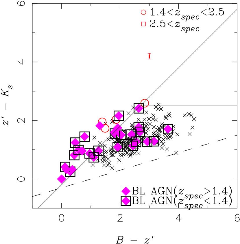
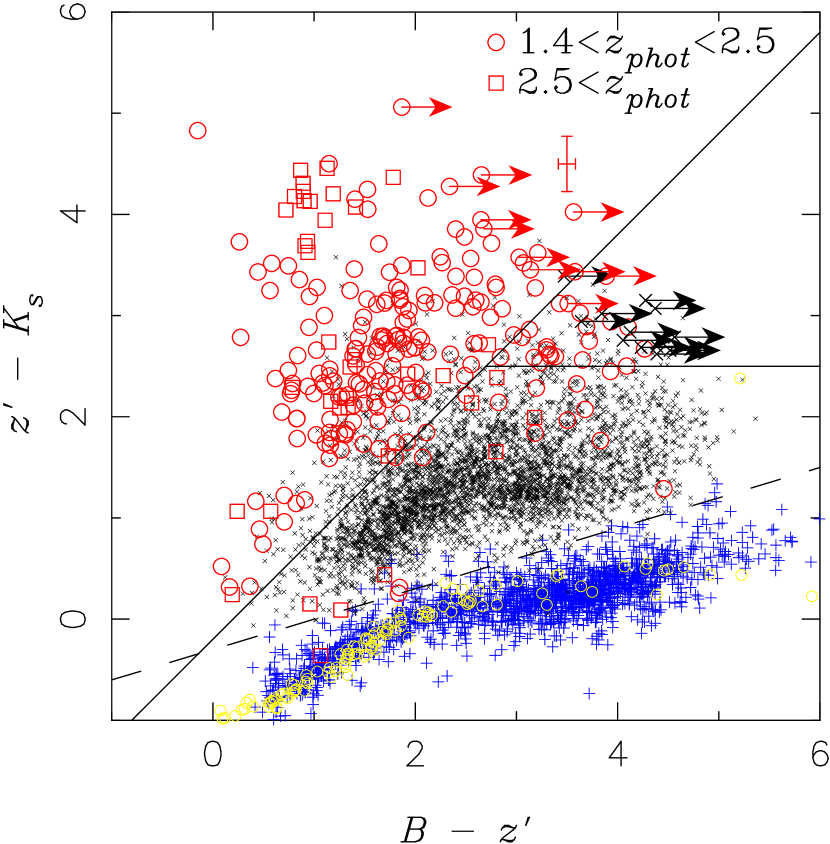
Figure 44: $BzK$ diagram in the field. Symbols of cross bar at $(B-z^{\prime},z^{\prime}-K_{s})=(3,4.5)$ represent typical errors of the color. Magenta diamonds represent BL AGNs, in which squared diamonds represent lower-redshifted ones at $z<1.4$. Left: For the spectroscopic samples, red circles represent sources at $z_{spec}=1.4-2.5$. Right: The same as on the Left for the photometric samples, where blue cross and yellow circles represent the stellar objects selected with the scheme described in subsection 3.4, respectively, and the reference stars of the BPGS star atlas. Red circles and squares represent sources at $z_{phot}=1.4-2.5$, and at $z_{phot}>2.5$ respectively.

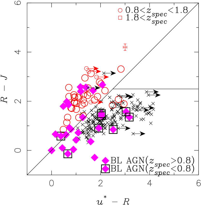
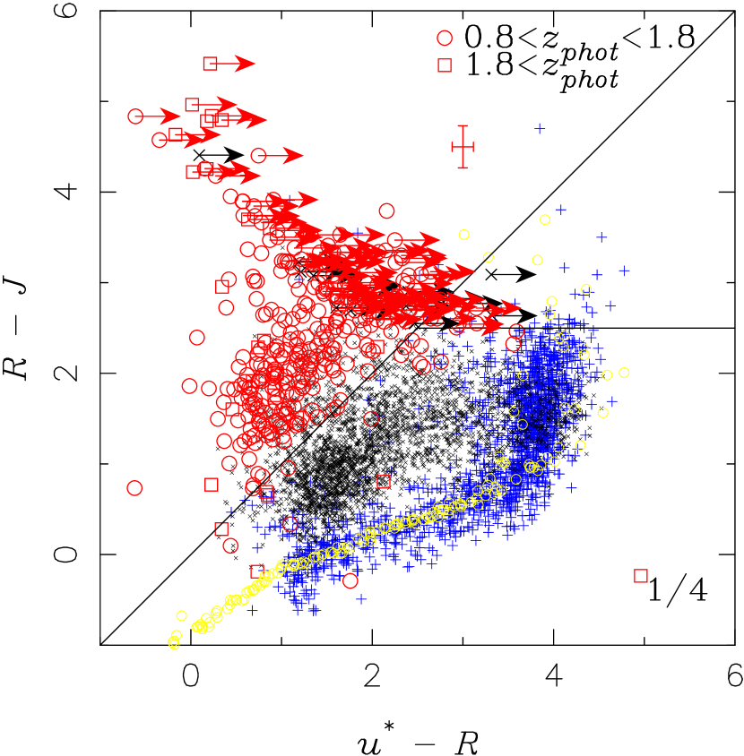
Figure 45: The same as figure 44 for the uRJs. Symbols of cross bar at $(u^{\ast}-R,R-J)=(3,4.5)$ represent typical errors of the color. Red circles and squares represent sources at $z_{phot}=0.8-1.8$ and at $z_{phot}>1.8$, respectively. Left: For the spectroscopic samples. Right: For the photometric samples. Only one fourth of all photometric sources detected in the $uRJ$ bands are plotted to reduce crowding in the diagram.

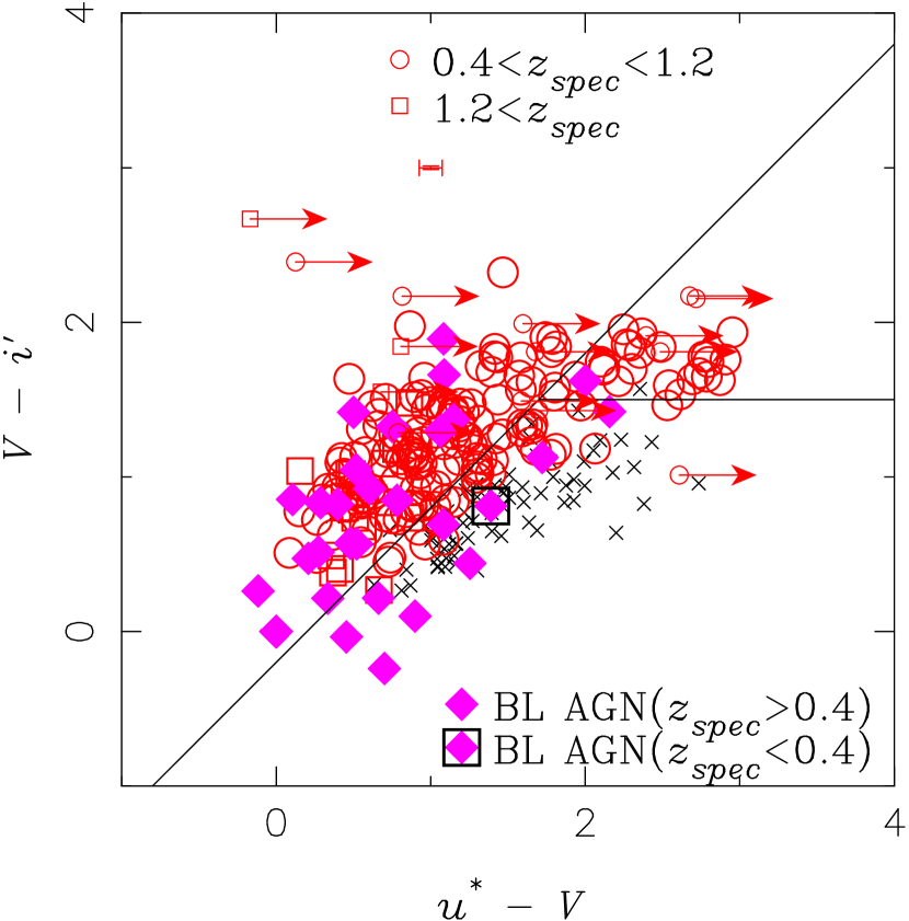
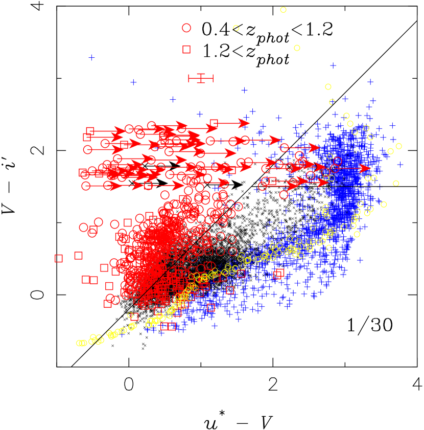
Figure 46: The same as figure 44 for the uVis. Symbols of cross bar at $(u^{\ast}-V,V-i^{\prime})=(1,3)$ represent typical errors of the color. Red circle and square represent sources at $z_{spec}=0.4-1.2$ and $z_{spec}>1.2$, respectively. Left: For the spectroscopic sample. Right: For the photometric sample. Only one thirtieth of all photometric sources detected in the $uVi$ bands are plotted to reduce crowding in the diagram.

Figure 47: Photometric redshift distributions for the BBGs in the field. The white, shaded, and dark area represent the s-, qp-, and p-BBGs, respectively. Left: For the classical BBGs. Right: The same as on the left for the extended BBGs. Left-Top: Lower, upper solid line and dashed line histogram represent the uVis, the $z^{\prime}$-detected galaxies, and the rest-frame $V$-detected galaxies, respectively. Left-Middle: For the uRJs. Left-Bottom: For the BzKs. Right: For the uRN3s. Right-Upper-Middle: For the BRN3s. Right-Lower-Middle: For the uzN3s. Right-Bottom: For the BzN3s.

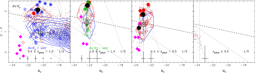
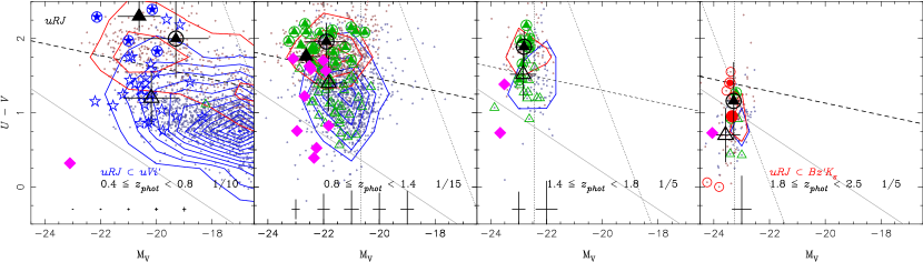
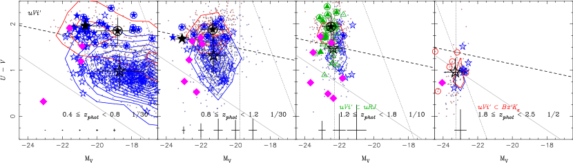
Figure 48: The same as figure 2 for classical BBGs. Typical errors of the magnitude and color are represented with crosses at the bottom. The vertical dotted and steep slope dotted lines represent the limiting absolute $V$ and $U$-band magnitudes at the mean redshift, respectively. In general, colored open, solid, and open-solid symbols represent objects classified as s-, p-, and qp-BBGs, respectively. Basically, red circles, green triangles, and blue stars represent objects selected with the two-color criteria as BzKs, uRJs, and uVis, respectively. Black-large open, solid, and open-solid symbols represent mean values for the s-, p-, and qp-BBGs, respectively. Crosses on the black symbols represent their standard deviations. Only a part of samples are plotted to reduce crowding in the diagram, whose fractions are presented as numbers in the right-bottom region of all figures. Top: The BzKs at $0.4\leq z<1.2$, $1.2\leq z<1.4$, $1.4\leq z<2.5$, and $z\geq 2.5$ are plotted from left to right. For BzKs also classified as uRJs at $1.2\leq z<1.4$, their symbols are changed to green triangles from red circles. For BzKs also classified as uRJs at $0.4\leq z<1.2$, the symbols are changed to blue stars from red circles. Middle: The uRJs at $0.4\leq z<0.8$, $0.8\leq z<1.4$, $1.4\leq z<1.8$, and $1.8\leq z<2.5$ are plotted from left to right. For uRJs also classified as BzKs at $1.8\leq z<2.5$, their symbols are changed to red circles from green triangles. For uRJs also classified as uVis at $0.4\leq z<0.8$, their symbols are changed to blue stars from green triangles. Bottom: The uVis at $0.4\leq z<0.8$, $0.8\leq z<1.2$, $1.2\leq z<1.8$, and $1.8\leq z<2.5$ are plotted from left to right. For uVis also classified as uRJs at $1.2\leq z<1.8$, their symbols are changed to green triangles from blue stars. For uVis also classified as BzKs at $1.8\leq z<2.5$, their symbols are changed to red circles from blue stars.

A.1 The $BzK$, $uRJ$, and $uVi$ color-color diagram

Daddi et al. (2004) proposed that $z>1.4$ star-forming BBGs (s-BBGs) should occupy the upper-left region in a two-color $B-z$ and $z-K$ ($BzK$) diagram, as the bluer and redder colors trace UV excess and the Balmer/4000 Å break feature, representing the star forming activity and the old stellar component, respectively. We could also show that the $BzK$ technique is efficient for selecting galaxies at $1.4<z_{phot}<2.5$, as illustrated in figure 44.

We will argue that this kind of two-color technique can be extended to selecting s-BBGs at certain redshift intervals with other sets of three photometric observed broad bands, in which their wavelengths are nearly in an equal ratio as a geometric series. By introducing ${\cal B}$, $\mu$, and ${\cal R}$ as their AB magnitudes of general bluer, medium, and redder bands, resepectively, and defining a two-color index ${\cal B}\mu{\cal R}$ generalized in $BzK$:

$${\cal B}{\mu}{\cal R}\equiv({\mu}-{\cal R})-h_{\scriptsize{{\cal B}\mu{\cal R}}}({\cal B}-{\mu}),$$ (31)

it follows that s-BBGs at certain redshift intervals can be selected by a criterion:

$${\cal B}{\mu}{\cal R}\geq f_{\scriptsize{{\cal B}\mu{\cal R}}},$$ (32)

and passively evolving BBGs (p-BBGs) can be selected with a criterion:

$${\cal B}{\mu}{\cal R}<f_{\scriptsize{{\cal B}\mu{\cal R}}}\ \cap\ ({\mu}-{\cal R})_{\mbox{\scriptsize{AB}}}>g_{\scriptsize{{\cal B}\mu{\cal R}}}\;.$$ (33)

Even though we can obtain only the upper limit in their ${\cal B}$ magnitudes, we can select quasi passively evolving BBGs (qp-BBGs) with a criterion:

$$({\mu}-{\cal R})_{\mbox{\scriptsize{AB}}}>g_{\scriptsize{{\cal B}\mu{\cal R}}}\;.$$ (34)

We confirm the validity of this generalized BBG technique as shown in figures 45 and 46. These generalized criteria are efficient ways to select photometric s/p/qp-BBGs at $0.8<z<1.8$ and $0.4<z<1.2$ in the field for the $uRJ$ and $uVi$ filter sets. These particular color criteria also allow efficient selections of the BBGs not only for $1.4<z<2.5$, but also $0.8<z<1.8$ and $0.4<z<1.2$.

In order to study the validity and physical meaning of the two-color criteria that are generalized from the phenomenologically established $BzK$ technique of Daddi et al. (2004), we used the BC03 models to reproduce the blue ${\cal B}-{\mu}$ and red colors ${\mu}-{\cal R}$ of model galaxies, which are described and shown in figures 57 and 58 in appendix E.2. The result from the stellar population synthesis study is essentially similar to the cases of BzKs, as summarized below.

In the redshift ranges for each BBG selection in table 6, the galaxies with ongoing star formation appear in the upper-left region ${\cal B}{\mu}{\cal R}\geq f_{\scriptsize{{\cal B}\mu{\cal R}}}$ of the generalized ${\cal B}{\mu}{\cal R}$ color diagrams. The duration of the star-formation (age) has little influence on the blue color ${\cal B}-{\mu}$, while the redder color ${\mu}-{\cal R}$ increases with age. Only very young starbursts with ages less than 10 Myr, and without underlying older stellar populations, are located around the lower-left region, falling just below the line of ${\cal B}{\mu}{\cal R}=f_{{\cal B}{\mu}{\cal R}}$. On the other hand, the colors of normal galaxies, obtained from the CWW SED templates, fall outside the color area of the BBGs in the redshift ranges for each of the BBG selections. This means that the generalized two-color criteria can also be used to exclude the lower-$z$ objects.

The reddening direction lies approximately parallel to the line defined by ${\cal B}{\mu}{\cal R}=f_{{\cal B}{\mu}{\cal R}}$, since the dust extinction can be approximately represented by a power-law function of wavelength, implying that the reddening is similar in the ${\cal B}-{\mu}$ and ${\mu}-{\cal R}$ colors for star-forming galaxies in the various redshift ranges. This means that the generalized criteria ${\cal B}{\mu}{\cal R}\geq f_{{\cal B}{\mu}{\cal R}}$ for selecting BBGs are also robust from their dust reddening.

Only a few galaxies are found as faint blue objects at ${\cal B}-{\mu}\simeq 0$, suggesting that purely un-reddened, star-forming galaxies are rare, not only for s-BzKs at $z\simeq 2$, but also s-uRJs at $z\simeq 1$. On the other hand, we could find some fraction of these nearly extinction-free populations in s-uVis at $z\simeq 0.6$.

Figure 47 shows the distributions of photometric redshifts $z_{phot}$ for all the $z^{\prime}$-detected galaxies and the BBGs. Total numbers of detected uRJs and uVis as the lower-z BBGs are greater than that of detected BzKs while the fractions of low-z interlopers in the uRJs and uVis are in the same order as those in the BzKs as shown in figure 47. Thus, all the BBG selections can be effective to exclude low-z interlopers at $z<0.4,z<0.6$, and $z<1.2$ with the $uVi$, $uRJ$, and $BzK$ criteria. These selected-out redshift ranges are consistent with the expected values of $z<0.4,z<0.8$, and $z<1.2$ from the stellar population models (see in appendix E). While the uVis are selected out at $z>1.2$ as expected with the model tracks (see in appendix E), the uRJs and BzKs gradually decrease in population at $z>1.2$, and $>1.6$ lower than expected. Low efficiency for BBG selections at the high redshift side may be caused from the shallowness of our ground-based NIR photometry. The limiting magnitudes of $J<21$ and $K_{s}<22$ with the KPNO/FLMG are shallow compared with studies for the BzKs in other survey fields (Kong et al. 2006; Lane et al. 2007; Quadri et al. 2007; Blanc et al. 2008). Thus, we take into account this limitation of the ground-based NIR photometry in the dataset when we study galaxies at $z\simeq 0.8-2$ as uRJs and BzKs. We try to overcome the limitation due to the shallow ground-based NIR photometry for the uRJs and BzKs. We further extend the two-color criteria used for detecting the Balmer in combination with AKARI NIR photometry as discussed in appendix A.3.

A.2 Rest frame color of the BBGs

It is worth comparing the classification with the two-color criteria detecting the Balmer break for the BBGs and their rest frame colors. As shown in the top and middle of figure 48, most of the BzKs at $1.2\leq z_{phot}<1.4$ are classified as uRJs while only a few of the uRJs at $1.4<z_{phot}<2.5$ are classified as BzKs. This is related to the shallowness in our ground based NIR photometry, which is not deep enough to select the population around $z\simeq 2$ as BzKs as remarked in the previous section. For our sample up to $z\simeq 2$, the uRJ criteria are more useful than the BzK criteria. We can see the bimodality even for the BBGs again as the boundary between the blue cloud and the red sequence is consistent with that by Bell et al. (2004), which are plotted as nearly horizontal dotted lines in figure 48. Even though the bimodality of BBGs at $z>1.2$ is not so clear compared with that at $z<1.2$, the mean colors of the s-BBGs and the p- and qp-BBGs, represented as black open symbols and solid and open-solid symbols in figure 48, are in the blue cloud region and in the red sequence, respectively. Thus, the uRJ and uVi criteria can reasonably classify the the star forming and the passively evolving populations as the s-BBGs and the p- and qp-BBGs at $z<1.8$ in the field at least. It confirms that the generalized BBG criteria are also useful in order to distinguish a star-forming population from a passively evolving one.

A.3 Salvaging BBGs from N3Rs at $z>0.8$

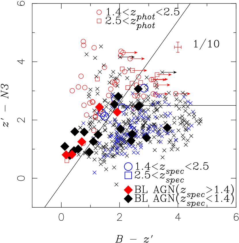
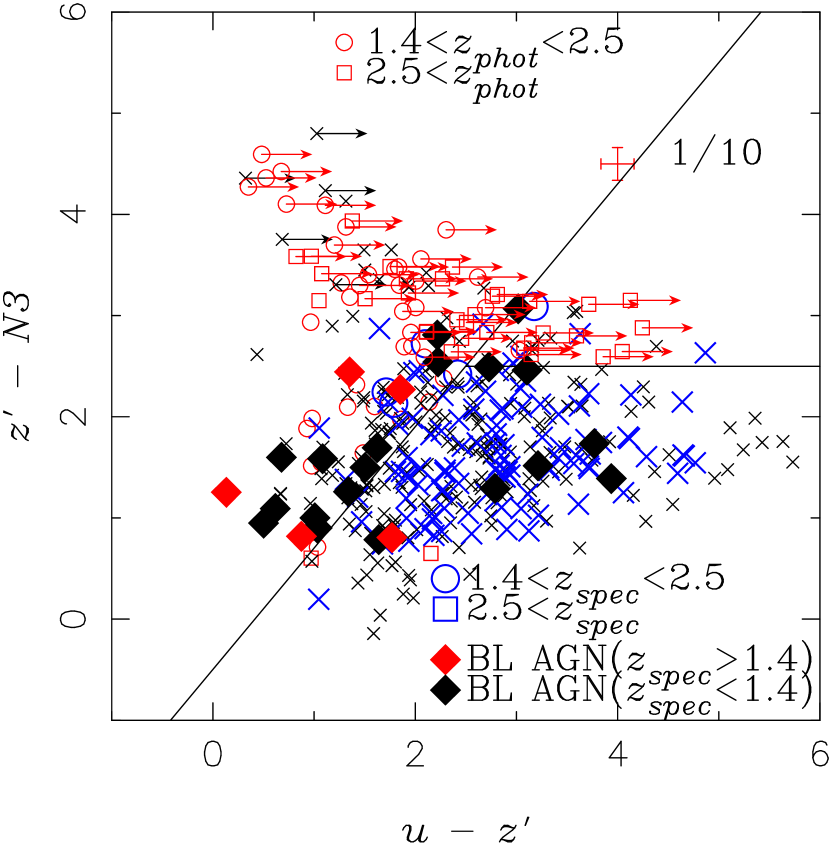
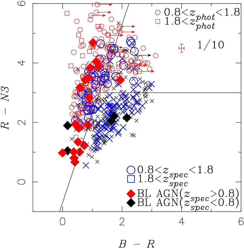
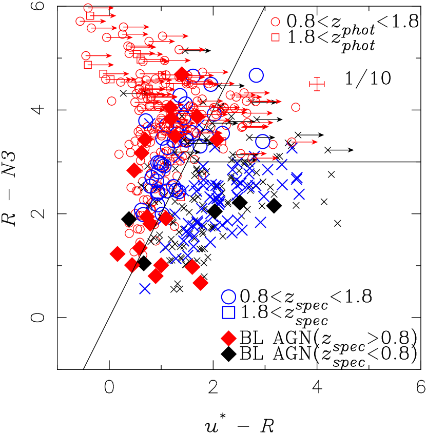
Figure 49: Two-color diagrams for the extended BBGs selected from the N3Rs, in which the $N3$ band is taken as the reddest band ${\cal R}$ in the BBG criteria. Red crosses at $({\cal B}-\mu,\mu-{\cal R})=(4,4.5)$ represent typical errors of the color. Only a part of the N3Rs are plotted to reduce crowding in the diagram, whose fractions are presented as numbers at $({\cal B}-\mu,\mu-{\cal R})=(5,4.5)$ in all figures. Diamonds represent BL AGNs. Large and small symbols represent the spectroscopic and the photometoric samples, respectively. Top-Left: The same as figure 44 for the BzN3s. Circles and squares represent objects at $z=1.4-2.5$ and $z>2.5$, respectively. Top-Right: The same as figure 44 for the uzN3s. Circles and squares represent objects at $z=1.4-2.5$ and $z>2.5$, respectively. Bottom-Left: The same as figure 45 for the BRN3s. Circles and squares represent objects at $z=0.8-1.4$ and $z\geq 1.4$, respectively. Bottom-Right: The same as figure 45 for the uRN3s. Circles and squares represent objects at $z=0.8-1.4$ and $z\geq 1.4$, respectively.

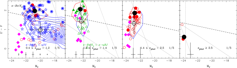
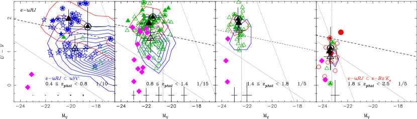
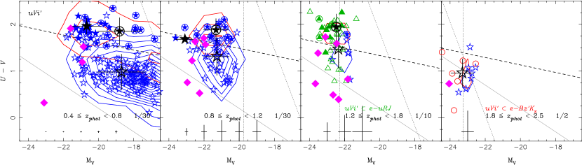
Figure 50: The same as figure 48 for all the BBGs, including the extended BBGs. Top: For all the BzKs, including uzN3s and BzN3s. For BzKs+uzN3s+BzN3s also classified as uRJs+uRN3s+BRN3s at $1.2\leq z<1.4$, their symbols are changed to green triangles from red circles. For BzKs+uzN3s+BzN3s also classified as uVis at $0.4\leq z<0.8$, their symbols are changed to blue stars from red circle. Middle: The same as on the left for all the uRJs, including uRN3s and BRN3s, as the Top. For uRJs+uRN3s+BRN3s also classified as BzKs+uzN3s+BzN3s at $1.4\leq z<2.5$, their symbols are changed to red circles from green triangles. For uRJs+uRN3s+BRN3s also classified as uVis at $0.4\leq z<0.8$, their symbols are changed to blue stars from green triangles. Bottom: The same as the Top for the uVis. For uVis also classified as uRJs+uRN3s+BRN3s at $1.2\leq z<1.8$, their symbols are changed to green triangles from blue stars. For uVis also classified as BzKs+uzN3s+BzN3s at $1.8\leq z<2.5$, their symbols are changed to red circles from blue stars.

As shown in appendix A, the BBG techniques employing not only the original $BzK$ color but also the $uRJ$ color can select galaxies around the redshift desert. However, we could not completely select these BBGs from the ground-based photometric dataset in the field since the ground-based $JK_{s}$ photometry with the KPNO/FLMG is not deep enough to pick up the IRBGs detected with the AKARI as seen in table 2. Since BBGs and IRBGs are almost the same populations at $z>0.4$ as discussed above, their statistics can confirm the limitation of the $JK$ depth. Roughly one third of N4Rs and N34 bumpers could not be identified as BzKs or uRJs as seen in the comparison between the left plot in figure 47 and the top-left plot in figure 4. Even though the limiting magnitude in the N3 band is comparable to those in J and K photometry as seen in table 2, the N3 band is effective to detect emissions around the rest-frame 1.6-$\mu$m IR bump for the objects at $z>1$ more than the J and K bands. In order to salvage these missing BBGs as non-BzK(non-uRJ) in N3Rs around the redshift desert, we used $N3$ photometry instead of the ground-based NIR ones for BBG selections with $BzN3/uzN3$ ($uRN3/BRN3$) colors as shown in figure 49. The numbers of salvaged BzN3s and uzN3s (uRN3s and BRN3s) were greater than those of BzKs(uRJs) even in this dataset as shown in figure 47. Hereafter, we often treat BzN3s and uzN3s (uRN3 and BRN3) as an extended BBG class of BzKs(uRJs) at $z\simeq 2$($z\simeq 1$) and call these BBGs selected by including the AKARI NIR photometry as extended BBGs while the BBGs selected only with the ground-based photometry as classical BBGs.

Appendix B Summary of classifications

Hereafter, we will summarize the photometric classification schemes introduced in the paper and show their outline as following tree diagrams, in which asterisk $\ast$, circle $\circ$, and star $\star$ at the front of a category represent a classification without using redshift information, with using redshift information, and with substituting photometric color conditions for redshift selections.

B.1 Optical classifications

$z^{\prime}$-detected galaxy        $\circ$ EBO        $\circ$ Rest-frame $V$-detected galaxy       red sequence  blue cloud   BBG        uVi       $\ast$s-uVi  $\ast$p-uVi  $\ast$qp-uVi   uRJ+(BRN3,uRN3)       $\ast$s-uRJ  $\ast$p-uRJ  $\ast$qp-uRJ   BzK+(BzN3,uzN3)       $\ast$s-BzK  $\ast$p-BzK  $\ast$qp-BzK

• $z^{\prime}$-detected galaxies: As shown in subsection 3.1, we selected $\sim$56000 of them, performed their photometry as summarized in table 2, and estimated $z_{phot},M_{\ast},A_{V}$, and $SFR_{opt;corr}$ as described in section 4 and appendix C.

• EBOs: The Extremely Blue Objects were selected with the criteria of equation (2), which are possibly AGNs as discussed in subsection 4.2 and appendix E.1.

• Rest-frame $V$-detected galaxy: We studied their stellar populations, which are subclassified as red sequence and blue cloud in the CMD with criteria (5) as discussed in subsection 4.2.

• BBGs: The Balmer Break Galaxies were introduced for redshift subclassifications of uVis, (e-)uRJs, and (e-)BzKs and distinction between star-forming (s-BBGs), passive (p-BBGs), and quasi-passive (qp-BBGs) populations with the criteria (32), (33), and (34) in appendix A.

B.2 NIR classifications

$z^{\prime}$-detected galaxy        $\ast$N3R        IRBG       $\ast$N23 bumper  $\ast$N34 bumper  $\ast$N4R   N3N4R     

• N3Rs: The N3 Red galaxies are selected from the $z^{\prime}$-detected galaxies by the criterion (6) in subsection 5, which roughly correspond to populations at $z>0.4$.

• IRBGs: The N3Rs were subclassified to the N23, N34 bumpers, and N4 Red galaxies (N4Rs) by the criterion (7) as InfraRed Bump Galaxies with 1.6 $\mu$m IR bump features from their stellar emissions.

• N23, N34 bumpers, and N4Rs: They approximately correspond to the uVis, e-uRJs, and e-BzKs, respectively.

• N3N4Rs: The N3N4 Red galaxies were classified by equation (12), which are possibly bright AGN candidates as discussed in subsection 6.2.

B.3 MIR classifications

$z^{\prime}$-detected galaxy        $\ast$N3 Red galaxy(N3R)        MbN3R        $\star$s-MbN3R       sb-MbN3R  s/a-MbN3R   $\star$agn-MbN3R        $\star$ MmN3R^#:6.3        $\star$pP-MmN3R       sb-pP-MmN3R  non sb-pP-MmN3R   $\star$fP-MmN3R       sb-fP-MmN3R  non sb-fP-MmN3R   $\star$MmN4R        $\star$MfN3R     

• MbN3Rs: The MIR bright N3Rs were selected from the N3Rs with the detection in more than two MIR bands, as described in subsection  6.1.

• s- and agn-MbN3R: The MbN3Rs were subclassified to starbursts (s-MbN3Rs) and AGNs (agn-MbN3Rs) by the MIR color criteria (8), (9), and (10) at $z=0.4-0.8,0.8-1.2$, and $>1.2$, respectively, as shown in figure 6.

• sb- and s/a-MbN3Rs: The s-MbN3Rs were subclassified to StarBurst-dominant (sb-MbN3Rs) and Starburst/AGN mixture(s/a-MbN3Rs) by their IR SED fittings.

• MmN3Rs: The MIR marginally-detected N3Rs were detected only in one or two MIR bands with SN3, which may be mimics of MbN3Rs with fainter MIR emission. They were subclassified the pP-, fP-, sb- and non sb-MmN3Rs as discussed in subsection 6.3.

• pP- and fP-MmN3Rs: The MmN3Rs were subclassified to the Possibly PAH emitting (pP-MmN3Rs) and the faint PAH (fP-MmN3Rs) populations as the PAH 7.7 um emission from the former is possibly dominant in $S11,L15$, and $L18$ bands at $z=0.4-0.65,0.65-1.5$, and $>1.5$ while that from the latter is not.

• sb- and non sb-MmN3Rs: The StarBurst-dominant populations (sb-MmN3Rs) have MIR SEDs which are reproduced by the S&K model with a low AGN mixture rate $<50\%$ while non sb-MmN3Rs do not.

• MfN3Rs: The MIR faint N3Rs were not detected in any MIR bands with SN3 as discussed in subsection 6.4.

B.4 Combining classifications

We have sometimes introduced subgroups by combining these optical, NIR, and MIR classifications. For example, the N3Rs, classified by the criteria of the IR bump in the NIR photometry, can be also subclassified into s-,p-, and qp-BBGs with the criteria of the Balmer break in the optical photometry, which were applied for the N3 Red BBGs as the exclusively classified BBGs from the N3Rs as seen in subsection 5.2. Thus, the combination of classifications at different wavelengths can help us in quickly studying galaxies.

Appendix C Photometric redshifts of various populations

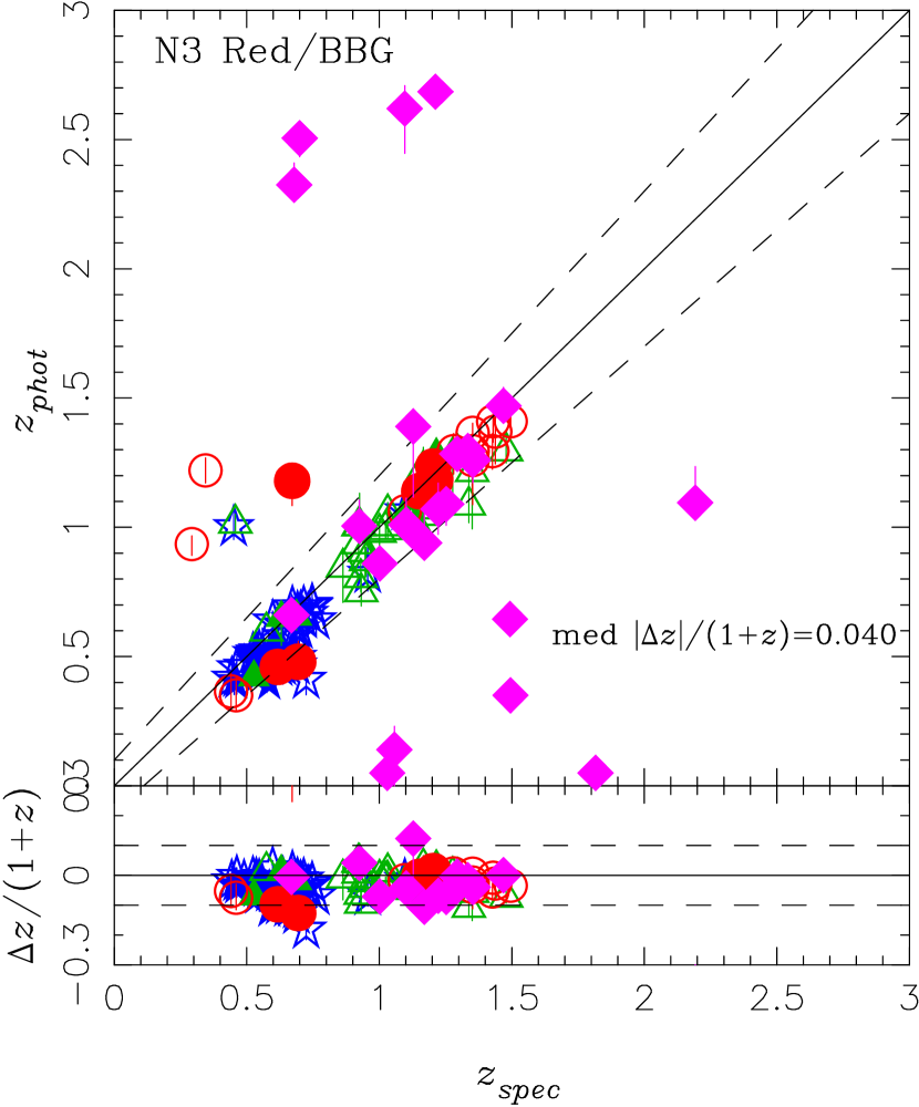
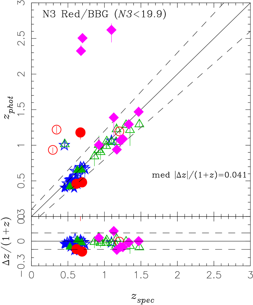
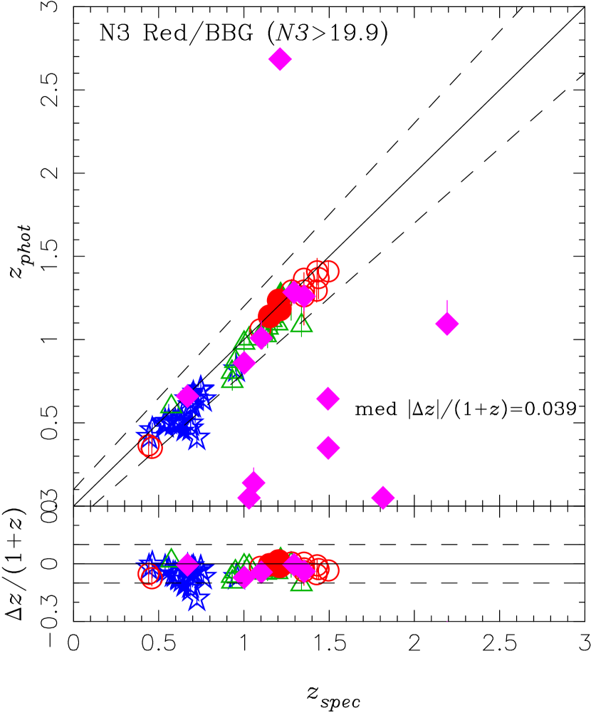
Figure 51: The same as figure 1 for the N3 Red BBGs. The colors and symbols are the same as figure 6. The magenta square means BL AGN classified with the spectroscopy. Top: For all the spectroscopic N3Rs. Bottom-Left: For reltaively bright N3Rs with $N3<19.9$. Bottom-Right: For relatively not-bright N3Rs with $N3\geq 19.9$.

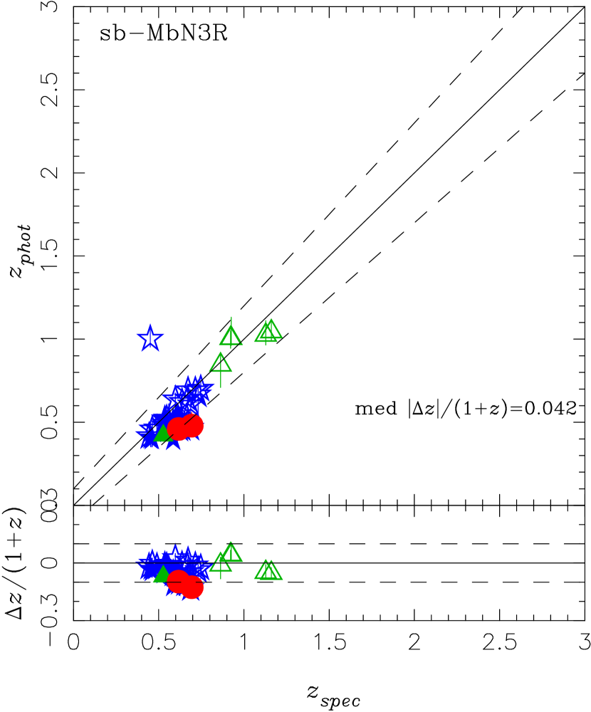
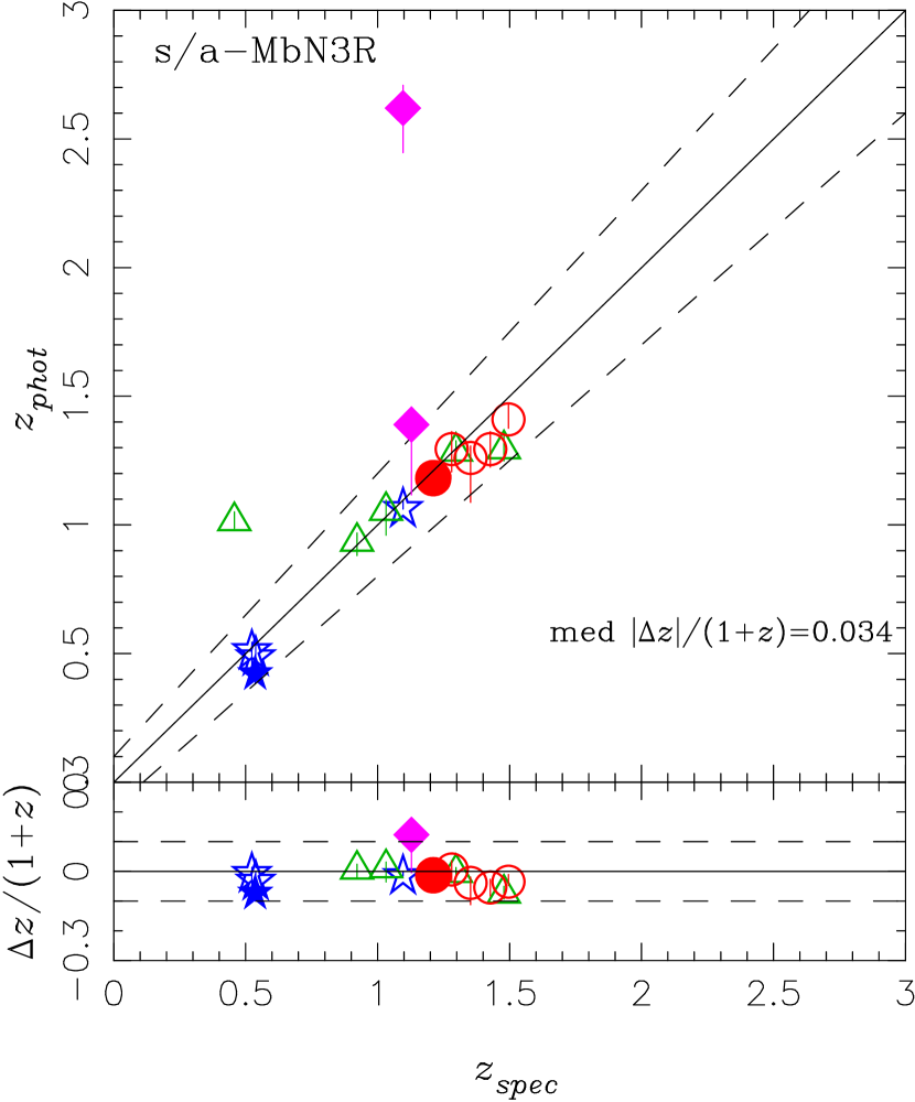
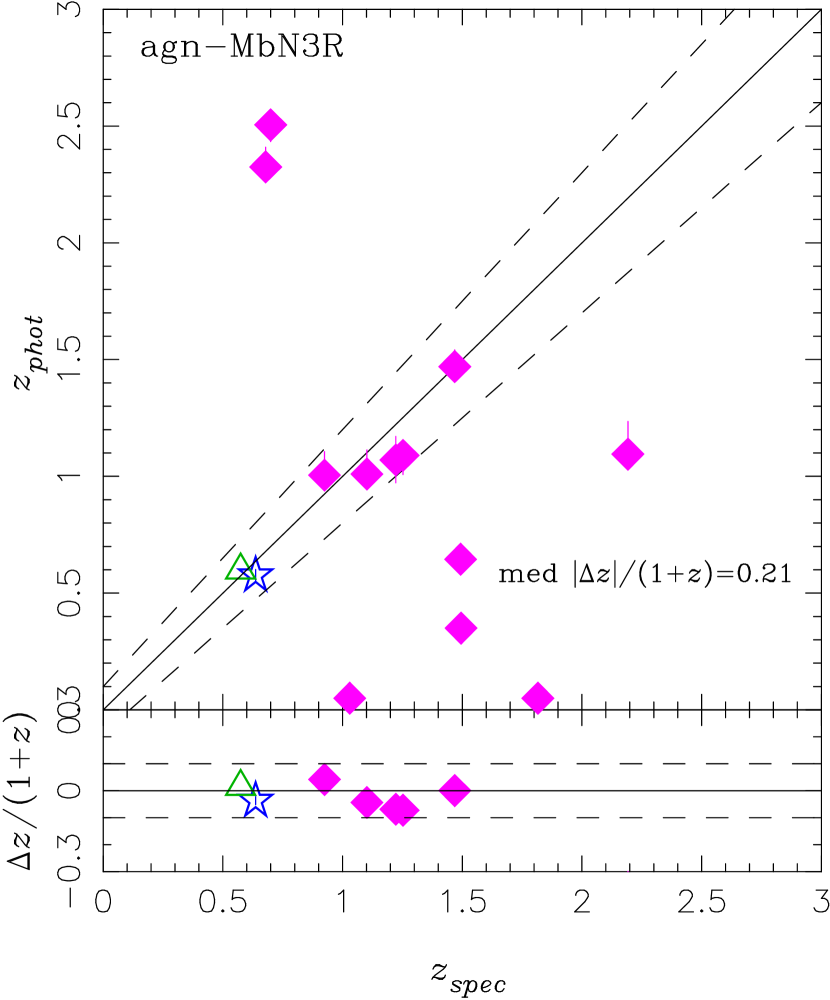
Figure 52: The same as figure 51 for the MbN3Rs; the sb-, s/a-, and agn-MbN3Rs from left to right, which are subclassified on the basis of their MIR SED features as shown in subsection 6.1.

We obtained the spectra of 83 N3Rs, in which MIR bright sources are subclassified into 35 sb-MbN3Rs, 9 s/a-MbN3Rs, and 14 agn-MbN3Rs. For these spectroscopic N3Rs and MbN3Rs samples, figures 51 and  52 show the redshift discrepancy $\Delta z=z_{phot}-z_{spec}$. The median accuracies of $\langle\Delta z\rangle/(1+z_{spec})$ are 0.040, 0.041, 0.039, 0.042, 0.034, and 0.21 for all the N3Rs, relatively bright N3Rs ($N3<19.9$), relatively faint N3Rs ($N3>19.9$), sb-MbN3Rs, s/a-MbN3Rs, and agn-MbN3Rs, respectively.

We can see no essential difference in the median accuracy between the relatively bright and faint N3Rs, which means that the brightness does not essentially affect the photometric redshift estimations. We can also see that sb-MbN3Rs, preselected for $z>0.4$ with the IR bump criterion $N2-N3>-0.3$, show good agreement between $z_{spec}$ and $z_{phot}$, which means that the photometric redshift estimation is still robust even under heavy extinctions in these MbN3Rs as long as one excludes low redshift dusty starbursts with the IR bump detection.

The agn-MbN3Rs show the largest discrepancy in all the subclasses in the N3Rs. It confirms that AGN is one major cause for inducing deviations in the photometric redshifts, which is reasonable since we used only stellar population synthesis modeled SEDs as BC03 without including AGN SEDs. Even though 14 spectroscopically observed agn-MbN3Rs, as candidates harboring AGNs, include 8 outliers, all the outliers are spectroscopically identified as BL AGNs and the remaining 6 non-outliers out of BL AGNs show that their median accuracy is comparable to that of the sb-MbN3Rs as $\langle\Delta z\rangle/(1+z_{spec})=0.042$. It suggests that their photometric redshifts can be accurately estimated from the SED fitting with their major stellar emission of the host galaxies even harboring AGNs.

Thus, the photometric redshifts for N3Rs and MbN3Rs can be used to reconstruct their redshifts.

Appendix D Redshift distributions of galaxies

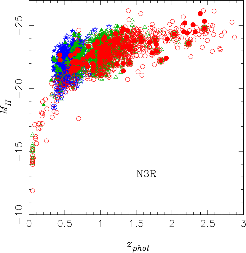
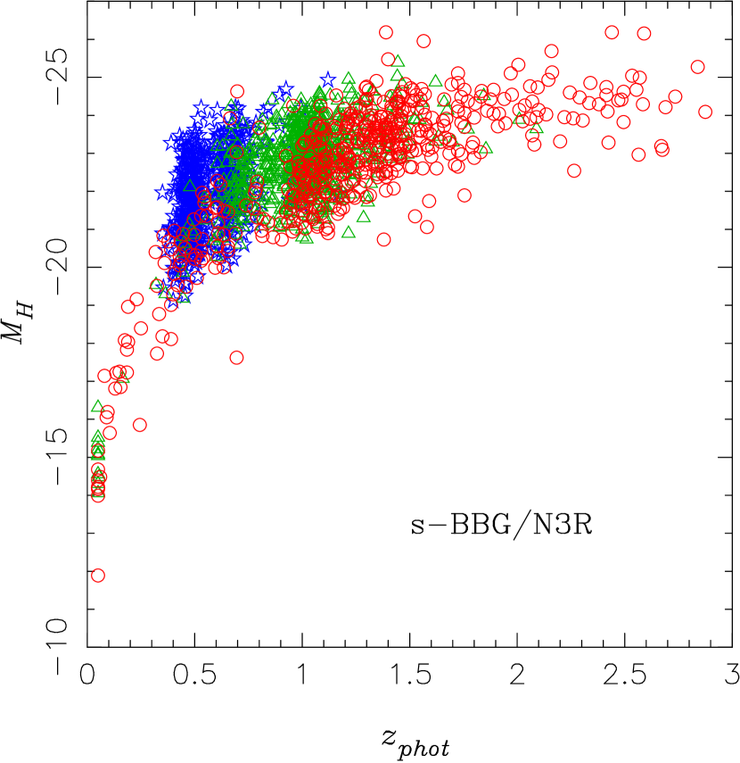
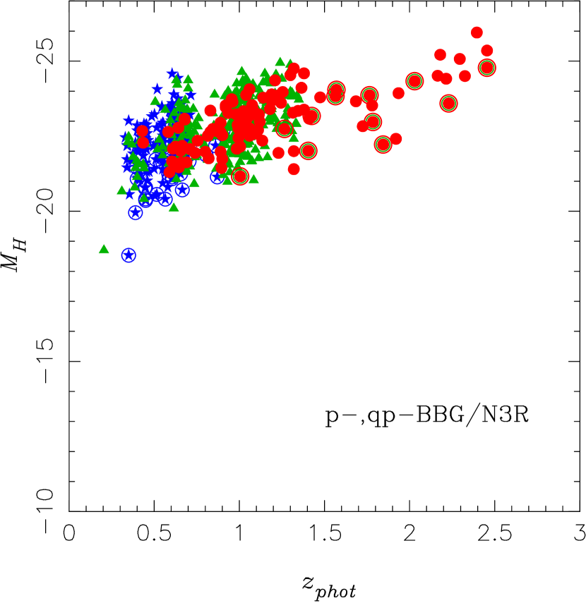
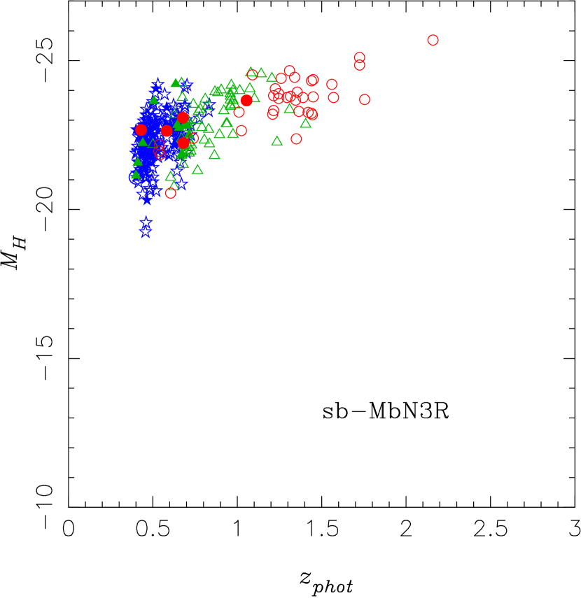
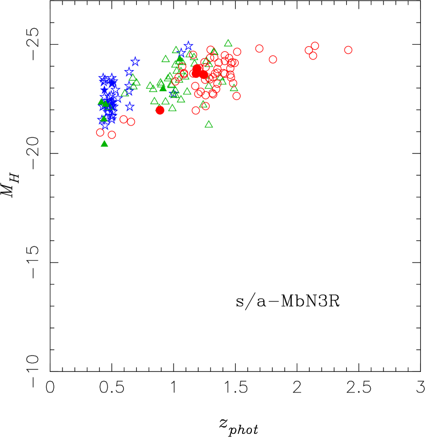
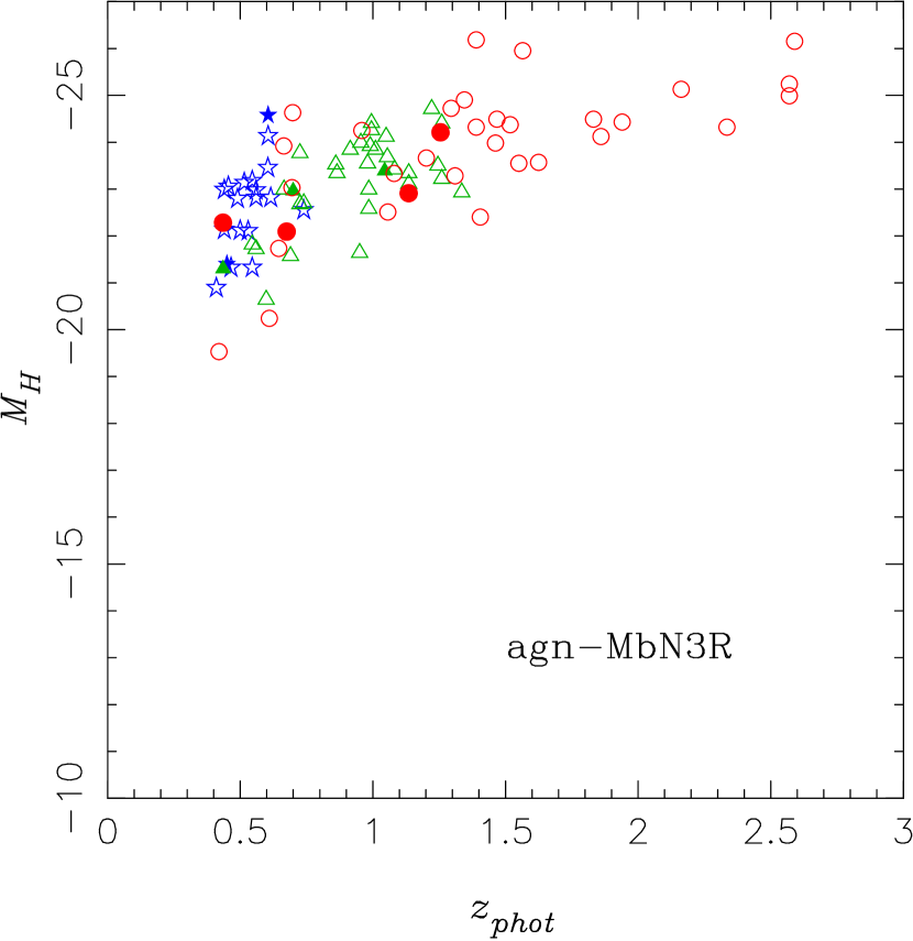
Figure 53: Photometric redshift $z_{phot}$ vs. rest-frame $H$ absolute magnitudes for N3Rs. The colors and symbols are the same as figure 6. Upper-Left: For all the N3Rs. Upper-Right: The same as the Upper-Left, for the IRBGs classified as s-BBGs. Middle-Left: The same as the Upper-Left, for the IRBGs classified as p-BBGs. Middle-Right: The same as the Top-Left, for the AKARI MIR detected IRBGs classified as sb-MbN3Rs. Bottom-Left: The same as the Top-Left, for the MIR detected IRBGs classified as s$/$a-MbN3Rs. Lower-Right: The same as the Upper-Left, for the MIR detected IRBGs classified as agn-MbN3Rs.

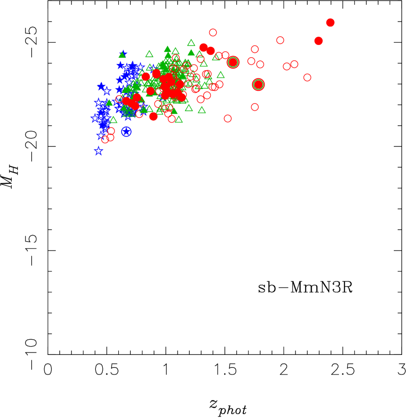
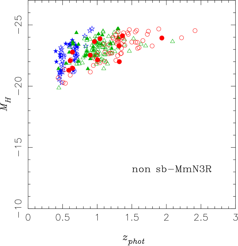
Figure 54: Photometric redshift $z_{phot}$ vs. rest-frame $H$ absolute magnitudes for the MmN3Rs. The colors and symbols are the same as figure 6. Left: For the sb-MmN3Rs. Right: For the non ab-MmN3Rs.

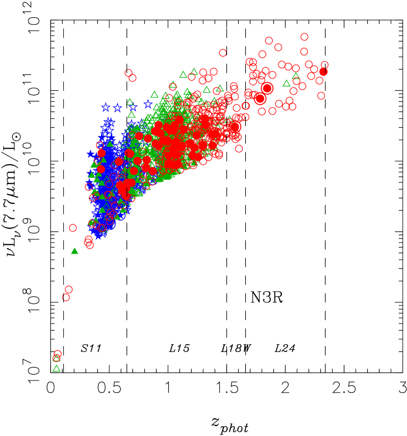
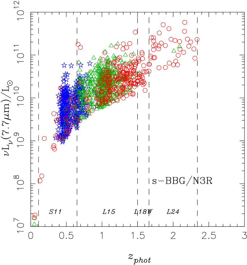
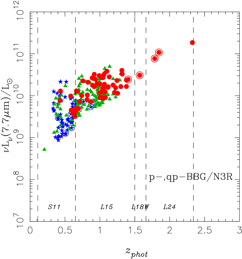
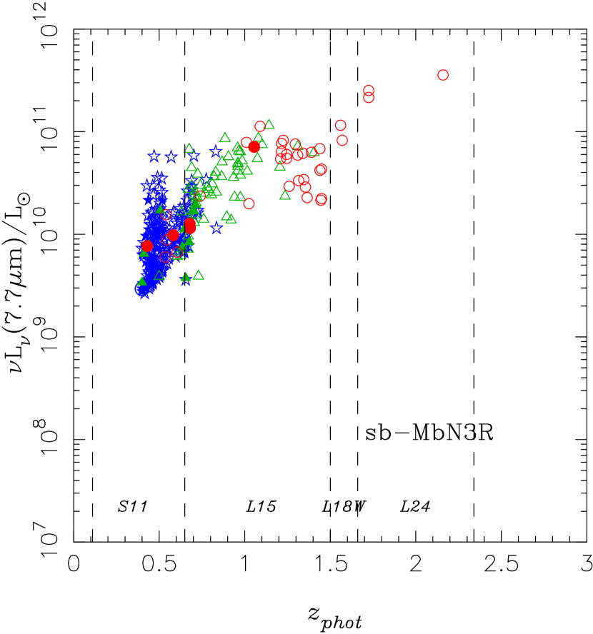
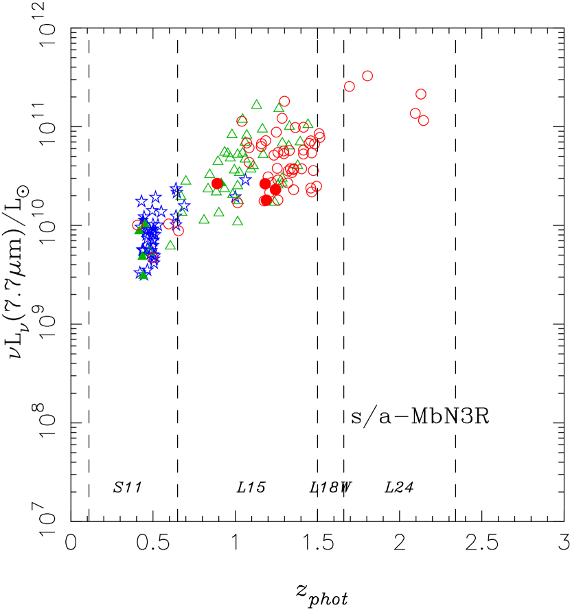
Figure 55: Photometric redshifts $z_{phot}$ vs. monochromatic luminosities $\nu L_{\nu}(7.7~{}\mu\mbox{m})$ at the rest frame 7.7 $\mu$m. The colors and symbols are the same as figure 6.

Figures 53,  54, and  55 show the photometric redshift $z_{phot}$ vs. rest-frame $H$ absolute magnitudes and monochromatic luminosities $\nu L_{\nu}(7.7~{}\mu\mbox{m})$. Following the conversion from rest-frame $H$ absolute magnitude to $M_{\ast}$ with equation (41) in appendix G, we can see that galaxies with $>10^{10}$M_⊙ are detected as the N3Rs at $z>1$ in figire 53. The standard nomenclature LIRG refers to a luminosity class of galaxies with $L\simeq 10^{11-12}L_{\odot}$ and is distinct from starbursts $L\simeq 10^{10-11}L_{\odot}$ and ULIRG $>10^{12}L_{\odot}$. Following the conversion from $\nu L_{\nu}(7.7~{}\mu\mbox{m})$ to TIR luminosity with equation (16) in subsection 7, we can see that most of the AKARI MIR-detected galaxies, classified as the s- and s/a-MbN3Rs and sb-MmN3Rs, have typically a TIR luminosity of $10^{11-12}L_{\odot}$, which corresponds to those of local LIRGs.

We can see also that the trend of agn-MbN3Rs is different from those of sb- and s/a-MbN3Rs.

Appendix E Models for SEDs and colors

E.1 Model tracks for extremely blue objects

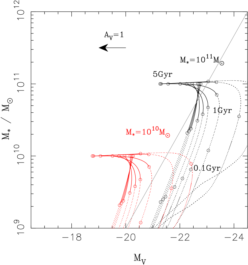
Figure 56: Left: The evolutionary tracks on the color-magnitude diagram of $M_{V}$ vs. $(U-V)$ from the BC03 models. Red and black lines correspond to systems with M${}_{\ast}=10^{10}$M_⊙ and M${}_{\ast}=10^{11}$M_⊙ at 5 Gyr, repsectively, which are evolving with exponential decaying SF with time scales of $\tau=$0.1, 0.3, 1,2, 3,5, 15, 30 Gyr and Constant Star Formation (CSF) from the left to the right on the diagram. All of them are in the cases without extinctions. The open circles represent ages of the systems of 0.1, 1, and 5 Gyr for all the models. An Arrow at the $(M_{V},U-V)=(-18,1)$ represents color-magnitude correction with a mean extinction $A_{V}\simeq 1$. Right: The same as on the left for the mass-magnitude diagram of $M_{V}$ vs. $M_{\ast}$ from the BC03 models.

As remarked in subsection 4.1, all the spectroscopic BL AGNs in the $z_{phot}$ outliers are also the EBOs with $(U-V)<-0.25(M_{V}+22.0)+0.7$, which suggests that most of the EBOs are possibly AGN candidates as long as the redshift estimation is unaffected even by SEDs with a mixture of stellar and AGN emissions. In order to confirm this assumption, we reconstruct the evolutionary tracks with the BC03 models on the CMD and the Magnitude vs. Stellar Mass diagram as shown in figure 56. Most of the observed star-forming galaxies suffer from extinctions $A_{V}\simeq 1$ as discussed in subsection 7.3. Thus, most normal star-forming galaxies with $A_{V}\simeq 1$, except young phase ones with age $<0.1$ Gyr, cannot appear in the EBO region of $(U-V)<-0.25(M_{V}+22.0)+0.7$ on the CMD. Even without any extinctions, only objects in an early star forming epoch $<1$ Gyr can have the color of the EBOs. It is not realistic to ingnore extinctions. Indeed, we found evidence for existing dust even in the EBOs with MIR emission as reported in subsection 4.1.

E.2 Model tracks for Balmer break galaxies

Figure 57: The evolutionary tracks in the $uRJ$ diagram from theoretical models the same as the Fig. 8 for the $BzK$ diagram in Daddi et al. (2004). The top-left panel shows continuous star formation model tracks for ages from 1 Myr to 2 Gyr and for E(B-V)=0, 0.3, 0.6. Top right panel has simple stellar population models for ages from 0.1 to 2 Gyr and no reddening. The bottom-left panel shows evolutionary models with various formation redshifts and SFR timescales and no reddening. At decreasing redshifts the tracks generally turn from bottom-left to top-right. The bottom-right panel show colors for the local templates of various galaxy types from Coleman et al. (1980). All models are plotted for the range $0.8<z<1.8$, except in the bottom-right panel where plots are for $0<z<0.8$. The limits and color ranges of all four panels reproduce those of figure 45, for direct reference.

Figure 58: The $uVi$ diagram the same as figure 57 except the redshift range. All models are plotted for the range $0.4<z<1.2$, except in the bottom-right panel where plots are for $0<z<0.5$. The limits and color ranges of all four panels reproduce those of figure 46, for direct reference.

Figure 59: The $BzN3$ diagram the same as figure 57 except the redshift range. All models are plotted for the range $1.4<z<2.5$, except in the bottom-right panel where plots are for $0<z<1.4$. The limits and color ranges of all four panels reproduce those of figure 49, for direct reference.

Figure 60: The $uzN3$ diagram the same as figure 59 except the redshift range. All models are plotted for the range $1.4<z<2.5$, except in the bottom-right panel where plots are for $0<z<1.4$. The limits and color ranges of all four panels reproduce those of figure 49, for direct reference.

Figure 61: The $BRN3$ diagram the same as figure 57 except the redshift range. All models are plotted for the range $0.8<z<1.8$, except in the bottom-right panel where plots are for $0<z<0.8$. The limits and color ranges of all four panels reproduce those of figure 49, for direct reference.

Figure 62: The $uRN3$ diagram the same as figure 59 except the redshift range. All models are plotted for the range $0.8<z<1.8$, except in the bottom-right panel where plots are for $0<z<0.8$. The limits and color ranges of all four panels reproduce those of figure 49, for direct reference.

In order to determine the criteria for selecting the Balmer break galaxies as shown in appendix A.1, we studied the model tracks on two-color diagrams of $uRJ$, $uVi$, $BzN3$, $uzN3$, $BRN3$, and $uRN3$ as shown in figures 57,  58,  59,  60,  61, and  62, respectively.

Top-left panels of all the figures represent the tracks of constant star-formation (CSF) for ages of $10^{-2}$, $0.1,0.2,0.5,1$, and 2 Gyr, various reddening with Calzetti’s extinction law, and solar metalicity. We can see that galaxies in such a redshift range with ongoing star formation are indeed expected to lie in the left-upper side region ${\cal B}{\mu}{\cal R}\geq f_{\scriptsize{{\cal B}\mu{\cal R}}}$ of the two-color diagrams. The duration of the star-formation (age) has little influence on the bluer color ${\cal B}-{\mu}$, while the redder color ${\mu}-{\cal R}$ increases with age due to the development of strong Balmer/4000 Å breaks falling in the ${\mu}$-band around these selecting redshift $z\simeq\langle z\rangle_{{\cal B}{\mu}{\cal R}}$. Very young bursts with ages less than 10 Myr without underlying older stellar populations would be located around the left-bottom region just below the line of ${\cal B}{\mu}{\cal R}=f_{{\cal B}{\mu}{\cal R}}$.

We will note that the reddening direction is approximately parallel to the critical line of criteria ${\cal B}{\mu}{\cal R}=f_{{\cal B}{\mu}{\cal R}}$ since dust extinction is approximately represented as a power-law function of the wavelength and it is implying that the reddening is similar in the ${\cal B}-{\mu}$ and ${\mu}-{\cal R}$ colors for star-forming galaxies in the selected redshift range. It means that the generalized criteria ${\cal B}{\mu}{\cal R}\geq f_{{\cal B}{\mu}{\cal R}}$ for selecting BBGs are also robust from their dust reddening.

Top-right panels of all the figures represent the tracks of simple stellar population (SSP) models after an instantaneous burst, in the two-color diagrams, for ages of $10^{-2},0.1,0.2,0.5,1$, and 2 Gyr, with no reddening, and solar metalicity. Their features are also similar to those in the BzKs as the tracks are similar to those of star-formings at young ages and begin to move to the region of p-BBGs at older ages of $\geq 1$Gyr. Even though some tracks for intermediate ages of $\sim 0.5-1$ Gyr are outside of the s/p-BBG regions, the extinction tends to make them redder as those found in the s/p-BBG region. Even though we should be cautious when applying SSP models with no reddening to the analysis for real galaxies, the results support that the generalized schemes for selecting s/p-BBGs might still be robust.

The left-bottom panels of all the figures show that the ${\cal B}{\mu}{\cal R}$ colors for galaxies with various formation redshifts are exponentially declining SFRs ($\tau=0.3$ and 1 Gyr), with no reddening and solar metalicity. The color evolution of galaxies formed at high redshifts is such that most objects move directly from the star-forming galaxy region to the passive galaxy region without crossing the bluer regions populated by $z<1.4$ objects.

The right-bottom panel of all the figures shows that the colors of normal galaxies are derived from the CWW templates of E-Sbc-Scd-Irregular galaxies (Coleman et al. 1980), which fall outside the color area of the BBGs for $z>0.8$($z>0.4$), respectively. It means that the generalized two-color criteria can work to exclude the lower-z interlopers.

E.3 Model Tracks for dusty starbursts and AGNs

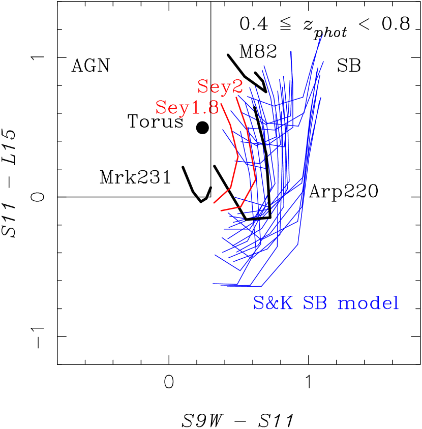
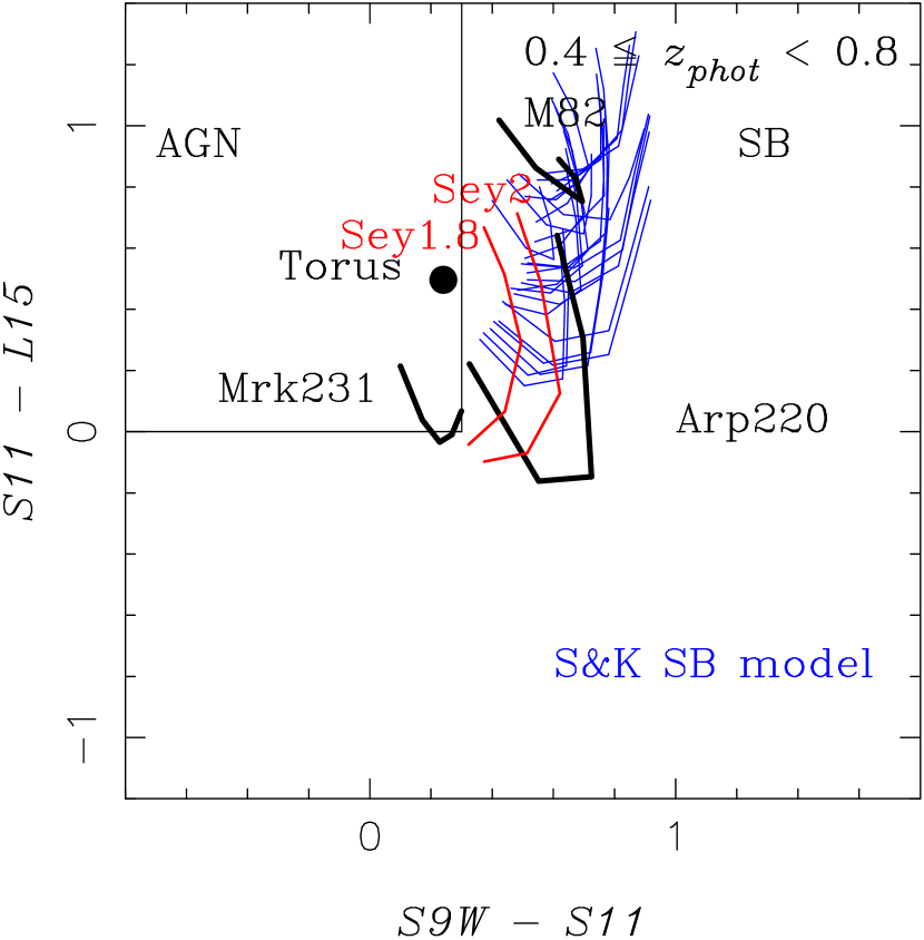
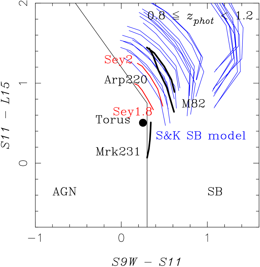
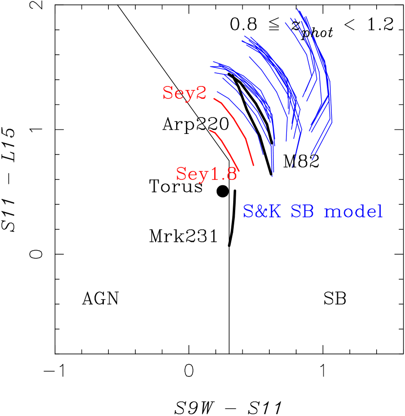
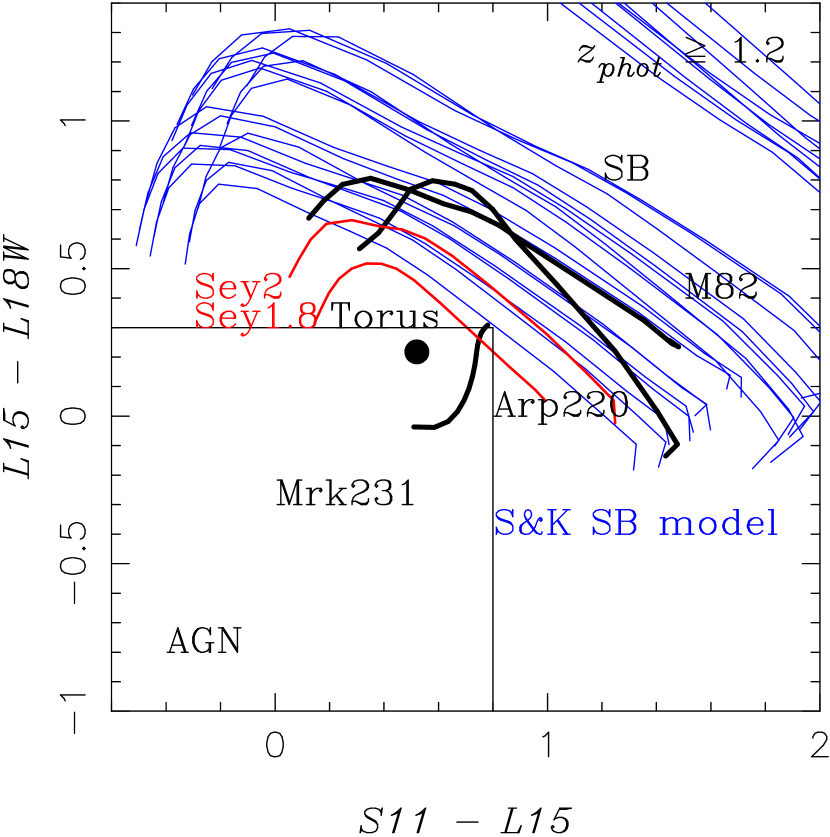
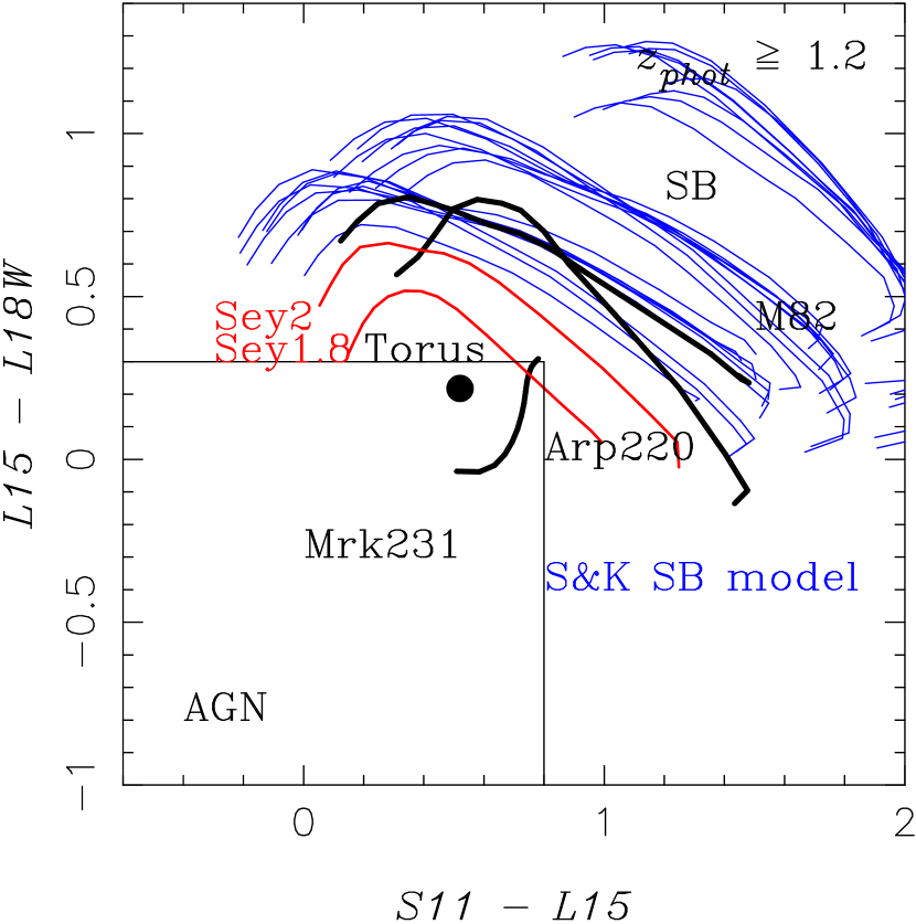
Figure 63: The MIR color-color diagrams for the model SEDs of LIRGs. Thin blue and solid black lines represent tracks for dusty starburst models, and observed (U)LIRGs: M82, Arp 220, and Mrk231. Blacked filled circle represents the dusty torus model of QSO2 in SWIRE SED templates. Objects in the left regions bounded with a thin solid line are excluded from starburst sample. Left: For the S&K model SEDs with a hot spot parameter of $n^{hs}=10^{2}(10^{4})\mbox{cm}^{-3}$. Right: The same as on the Left for $n^{hs}=10^{4}\mbox{cm}^{-3}$. Top: The $S9W-S11$ vs. $S11-L15$ diagram with the model tracks in the interval $0.4<z<1.0$. Middle: The same as the Top-Left, with the tracks in $0.8<z<1.4$. Bottom: The $S11-L15$ vs. $L15-L18W$ diagram with the tracks in $1.0<z<2.8$.

In figure 63, the thin blue curves, thick solid black curves, and black filled circles represent the redshifted tracks of dusty starburst SEDs of models by Siebenmorgen & Krügel (2007), SEDs of Arp220, M82 and Mrk231, and a model torus SED used to fit the SED of a heavily obscured type 2 QSOs SWIRE J104409.95+585224.8 (Polletta et al. 2006), respectively. As shown in figure 63, all the dusty starbursts of S&K models, Arp220, and M82 appear in the right area while the AGNs, including Mrk231 as an obscured AGN, appear in the left area. Thus, dusty starburst dominant LIRGs can be distinguished from AGN dominant LIRGs on the MIR color diagrams with a boundary represented as solid lines, which are introduced with equation (8) at $z=0.4-1.0$, equation (9) at $z=0.8-1.4$, and equation (10) at $1.0<z<2.8$ in section 6.

E.4 IR SED models

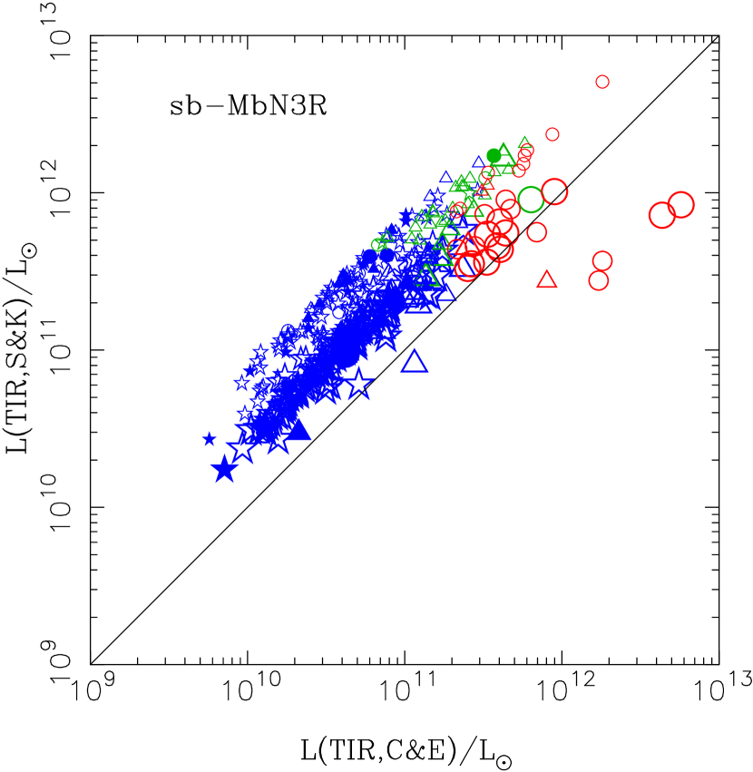
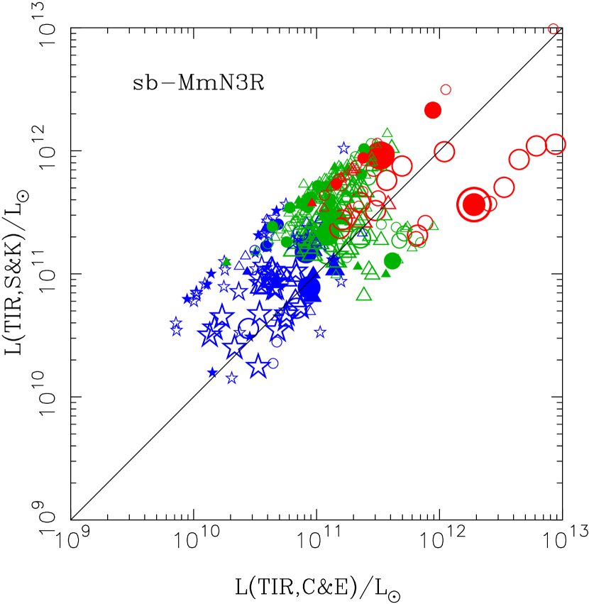
Figure 64: Comparison between TIR luminosities $L_{IR}$ estimated from the C&E model and the S&K model for the sb-MbN3Rs and the sb-MmN3Rs. Symbols are the same as in figure 6 except their colors. Blue, green, and red symbols represent the redshifts of $0.4\leq z<0.8$, $0.8\leq z<1.2$, and $z\geq 1.2$, respectively. Large, medium, and small symbols indicate the results which fit well with the S&K model SEDs of $A_{V;SK}=2.2,6.7$, and $17.9$, respectively. Left: For the sb-MbN3Rs. Right: For the sb-MmN3Rs.

With integrating a fitted model SED in rest-frame 8-1000 $\mu$m wavelength and correcting for the photometric redshift $z_{phot}$, we can obtain the total IR (TIR) luminosity $L_{IR}$ of the emission from the dusty star forming regions. There are various IR SED models. IR SED libraries can be prepared with three different kinds of schemes: 1) using SED templates of known galaxies (Laurent et al. 2000; Lutz et al. 2003; Spoon et al. 2004), 2) reproducing the SED with optical thin emission from the dusts assumed to be heated in a given radiation field without radiative transfer calculations (Chary & Elbaz 2001; Dale & Helou 2002; Lagache et al. 2003), and 3) calculating radiative transfer to evaluate the emission reprocessed with dusty medium in a spheroidal shape (Silva et al. 1998; Efstathiou et al. 2000; Takagi et al. 2003; Dopita et al. 2006; Piovan et al. 2006b, a; Siebenmorgen & Krügel 2007), or a general three dimensional shape (Kylafis & Bahcall 1987; Popescu et al. 2000), using ray tracing or Monte Carlo techniques (Bianchi et al. 2000). Even in scheme 3), the interaction between dust and radiation is treated consistently in Takagi et al. (2003) and Siebenmorgen & Krügel (2007). Even though empirical conversions from a monochromatic IR luminosity have been sometimes used, their empirical laws have been frequently derived from the SED fitting (Bavouzet et al. 2008). When we choose to use them, we should take into account their conceptional differences and applicable situations along with their limitations.

In order to extract information related to the physical properties in a dusty star-forming nucleus such as optical depth and dust density from the MIR SEDs with PAH emissions and Si absorption, in this paper, we have taken the S&K model. This can be used to prepare prepare MIR SEDs not only with various PAH emssion strengths but also Si absorption depth mainly parametrized with radiation field strength and optical depth, respectively. Individual SED features in the S&K model depend on the following parameters; total luminosity $L^{tot}$ L_⊙, size of starbursting nucleus $R$ kpc visual extinction $A_{V;SK}$, ratio of OB star luminosity with hot spots to the total luminosity $L_{OB}/L^{tot}$, and hydrogen number density in the hot spots $n^{hs}$. Even though the S&K model depends on the luminosity $L^{tot}$, we have scaled luminosities and used only their features in the MIR SED fittings. The parameters $L^{tot}$, $R$, and $A_{V;SK}$ have some degeneracy for variations of the MIR SED features. As shown in the comparison between figures 63,  6, and  11, the models with a hot spot parameter $n^{hs}=10^{2}\mbox{cm}^{-3}$ can cover typical MIR colors of MbN3Rs and MmN3Rs while the model with $n^{hs}=10^{4}\mbox{cm}^{-3}$ cannot. Thus, we have fixed the hot spot parameter with $n^{hs}=10^{2}\mbox{cm}^{-3}$. And, we have used its 27 models fixed with $R=3$kpc and parametrized with $L^{tot}=10^{10.1},10^{11.1}$, and $10^{12.1}$L_⊙, $A_{V;SK}=2.2,6.7$, and $17.9$, and $L_{OB}/L^{tot}=0.40,0.60$, and $0.90$, which are treated as only qualitative parameters to reproduce varieties in the MIR SEDs, not as quantitative parameters describing an exact physical state in the starburst nucleus.

In fact, the conversion from $\nu L_{\nu 7.7}$ to $L_{IR}$ depends on the IR SED models used in the fitting. For an example, as shown in figure 64, for most of the sb-MbN3Rs and MmN3Rs, we can see that the estimated $L_{IR;SK}$ from the SED fitting with the S&K model is approximately larger by a factor of three than those with the Chary & Elbaz model (hereafter C&E model). The IR emission at $>10~{}\mu$m in most of the S&K model SEDs dominate more than those in the C&E model, which causes the TIR luminosity $L_{IR;SK}$ estimated from the S&K model to be larger than the $L_{IR;CE}$ from the C&E model. The S&K model tends to derive larger TIR luminosity ratio of $L_{IR;SK}/\nu L_{\nu 7.7}$ when SEDs are fitted well with larger $A_{V;SK}$ even for samples with the same $\nu L_{\nu 7.7}$. On the other hand, the C&E model derives almost the same TIR luminosity ratio $L_{IR;CE}/\nu L_{\nu 7.7}$ for them. Thus, the difference among the three model parameters for $A_{V;SK}$ appears as the split multi-sequences in figure 64. Figure 64 shows multi-sequences with different ratios $L_{IR;SK}/L_{IR;CE}$ and $A_{V;SK}$ more clearly than figure 17.

In order to reproduce the dependence of the optical depth to derive TIR luminosity in the paper, we have used the templates in the public library by Siebenmorgen & Krügel (2007) while the analysis with Takagi et al. (2003), for MIR detected objects in the field, are also reported in other papers (Takagi et al. 2007, 2010).

Appendix F Error estimations

With photometric redshifts, we have derived physical values for the detected galaxies as absolute magnitudes $M$, monochromatic luminosities $\nu L_{\nu}$, stellar mass $M_{\ast}$, and SFR. The physical values include errors from not only their photometric fluctuation $\Delta m$ in the observed band but also uncertainty of their photometric redshift. In their error estimations, we have assumed that the former and the latter are independent of each other.

Absolute magnitudes $M$ is defined with luminosity $L_{\nu}$, observed magnitude $m_{\nu}$ and flux $F_{\nu}$ at the observed frequency $\nu$ as

$$M = -2.5\log_{10}\frac{L_{\nu}}{4\pi d_{L}(10\mbox{pc})}-48.6\;,$$ (35)

$$L_{\nu} = 4\pi d_{L}(z)^{2}\frac{F_{\nu}}{(1+z)}\;,$$ (36)

$$F_{\nu} = 10^{-0.4(m_{\nu}+48.6)}\;,$$ (37)

where $d_{L}$ is the luminosity distance. Thus, since $M=-2.5\log_{10}F_{\nu}-2.5\log_{10}\frac{d_{L}(z)^{2}}{(1+z)}+\mbox{const}$ with $f(z)=d_{L}(z)^{2}/(1+z)$, we estimate the error of absolute magnitudes $M$ as

$$\Delta M=\sqrt{\Delta m_{\nu}^{2}+\left(1.09\frac{\Delta f(z)}{f(z)}\right)^{2}}\;,$$ (38)

where we used $d(\log_{10}x)=(\log_{e}10)^{-1}dx/x=0.434dx/x$ and $\Delta m_{\nu}=1.09\Delta F_{\nu}/F_{\nu}$.

For the monochromatic luminosities $\nu L_{\nu}$ and the stellar mass $M_{\ast}$, with the similar schemes, their errors can be derived as

$$\Delta(\log_{10}\nu L_{\nu}) = 0.4\sqrt{\Delta m_{\nu}^{2}+\left(1.09\frac{\Delta f(z)}{f(z)}\right)^{2}}\;,$$ (39)

$$\Delta(\log_{10}M_{\ast}) = 0.4\sqrt{\Delta m_{K}^{2}+\left(1.09\frac{\Delta f(z)}{f(z)}\right)^{2}}\;,$$ (40)

where we used the error $\Delta m_{K}$ in $K$ band for the stellar mass error estimation.

In the error estimations for $SFR_{UV}$ and $SFR_{IR}$, we have used errors $\Delta m_{\nu}$ in the $u$ band and the IRC band related to the rest-frame 7.7 $\mu$m, respectively.

Appendix G Stellar mass from Optical/NIR SEDs

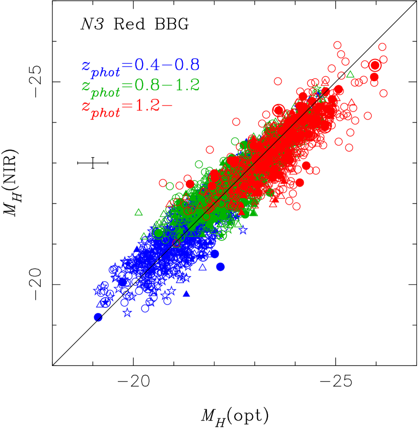
Figure 65: Comparison of the rest-frame $H$-band magnitudes for the N3 Red BBGs between $M_{H;NIR}$ and $M_{H;opt}$, which are derived from the AKARI NIR photometry and the ground-based optical-NIR SED fitting, respectively. Symbols are the same as in figure 6 except their colors. Blue, green, and red symbols represent the redshifts of $0.4\leq z<0.8$, $0.8\leq z<1.2$, and $z\geq 1.2$, respectively.

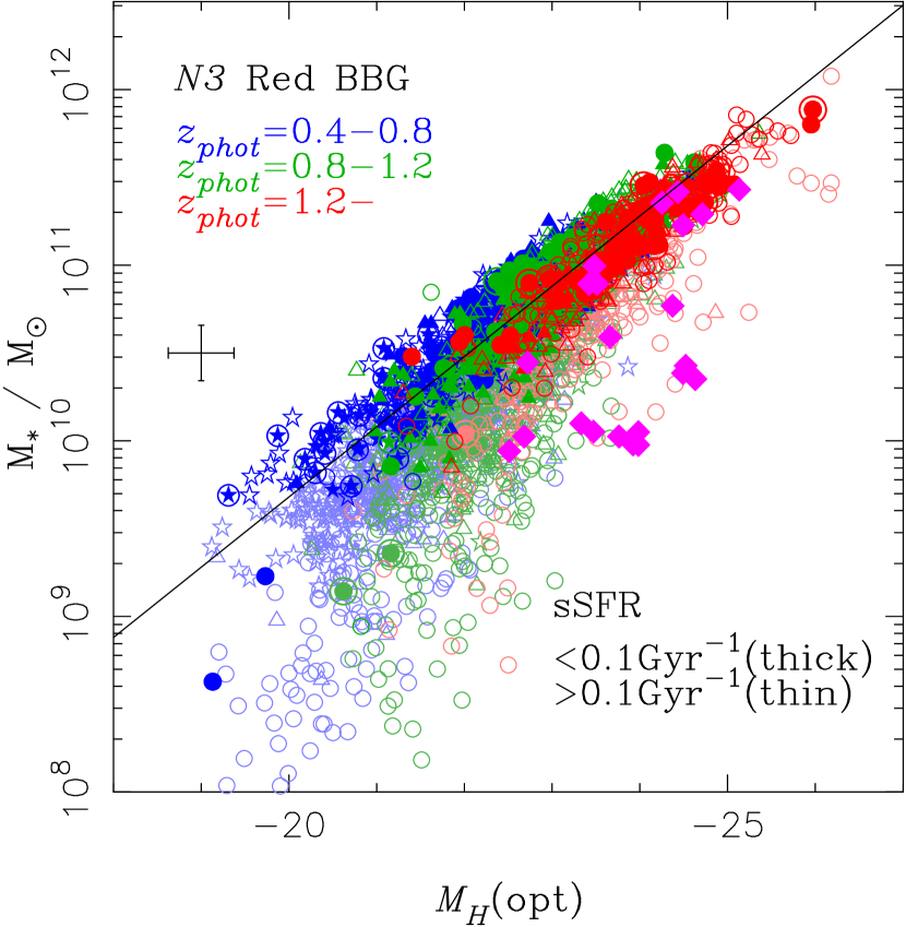
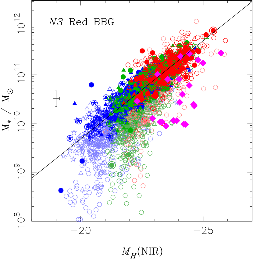
Figure 66: The absolute rest-frame $H$-band magnitude $M_{H}$ vs. stellar mass $M_{\ast}$ derived from the optical-NIR SED fitting, for all the N3 Red BBGs. Symbols are the same as in figure 65. The dark and faint colored symbols represents the subpopulation with sSFR $<0.1\mbox{Gyr}^{-1}$ and sSFR $>0.1\mbox{Gyr}^{-1}$. Left: The $M_{H;opt}$ reproduced from the BC03 model fitting vs. $M_{\ast}$. Right: The $M_{H;NIR}$ interpolated from the AKARI NIR photometry vs. $M_{\ast}$.

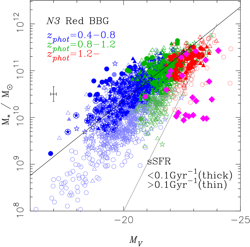
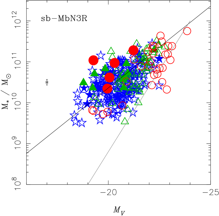
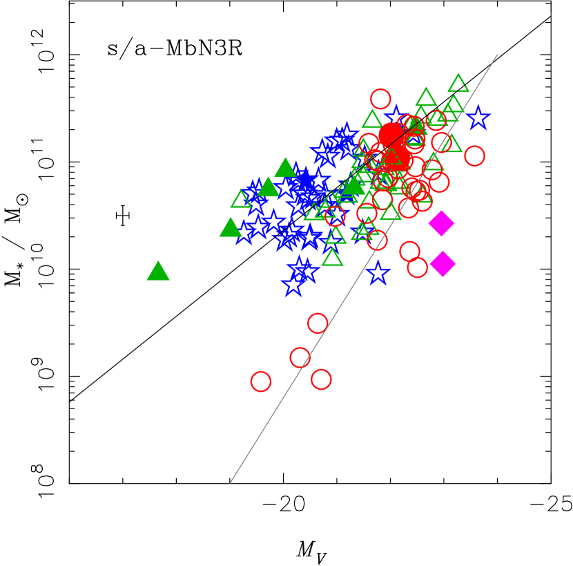
Figure 67: The absolute rest-frame $V$-band magnitude $M_{V}$ vs. stellar mass $M_{\ast}$ derived from the optical-NIR SED fitting. Symbols are the same as in figure 6 except their colors. Blue, green, and red mean the redshifts of $0.4\leq z<0.8$, $0.8\leq z<1.2$, and $z\geqq 1.2$, respectively. Magenta diamond represents the spectroscopic BL AGN. Steep line at the right side represents the boundary of the EBOs. Top-Left: All the N3 Red BBGs with $sSFR<0.1\mbox{Gyr}^{-1}$ and $>0.1\mbox{Gyr}^{-1})$ are represented with dark and thin symbols, respectively. Top-Right: For the sb-MbN3Rs. Bottom-middle: For the s/a-MbN3Rs. Bottom-Right: For the agn-MbN3Rs.

The stellar mass $M_{\ast}$ is estimated in a standard way with the optical-NIR SED fitting for all the $z^{\prime}$-detected galaxies and an alternative way from the AKARI/NIR photometry for the IRBGs as a subclass in the $z^{\prime}$-detected galaxies.

The rest-frame $H$ band wavelength corresponds to the rest-frame 1.6-$\mu$m IR bump where the emission is dominated by the stellar components in galaxies. It means that the absolute magnitude in rest-frame $H$-band $M_{H}$ represents the underlying stellar mass content $M_{\ast}$. This provided us with two ways to estimate the $M_{H}$ with our dataset; 1) the direct estimation from the AKARI/IRC photometry in the rest-frame $H$-band at 1.6 $\mu$m, and 2) the SED fitting with the ground-based photometric data.

First, the $N2,N3$, and $N4$ photometry can directly detect the 1.6-$\mu$m bump from the AKARI/IRC detected IRBGs even at $z>0.4$. Using the interpolation scheme with equation (4) for the $N2,N3$, and $N4$ photometry with $\lambda_{0}=1.6~{}\mu$m and $z=z_{phot}$, we can estimate the absolute magnitude $M_{H;NIR}(z_{phot})$ corresponding to the rest-frame $H$-band directly from the $N2,N3,\mbox{and}N4$ magnitudes of the AKARI/IRC detected IRBGs.

Second, the model fitting of Bruzual & Charlot (2003), with the whole ground-based $u^{\ast}BV$$Ri^{\prime}z^{\prime}$$JK_{s}$ SED, derives the absolute magnitude $M_{H;opt}$ with our small modified version of the hyperz as instantaneously deriving the photometric redshift $z_{phot}$ in subsection 4.1. It can apply for all the $z^{\prime}$-detected galaxies. Thus, the derived $M_{H;opt}(z_{phot})$ from the optical-NIR SED fitting with the ground-based photometric data is an alternative to determine the stellar mass $M_{*}$.

The absolute magnitude $M_{H;opt}(z_{phot})$ from the optical-NIR SED fitting is well correlated with that $M_{H;NIR}(z_{phot})$ from the $N2,N3$, and $N4$ photometry as shown in figure 65. Note this rest-frame $M_{H;NIR}(z_{phot})$ from the AKARI/NIR data can be approximately independent to the $M_{H;opt}(z_{phot})$ from the ground-based optical/NIR data, except for the photometric redshift $z_{phot}$ derived from the optical dataset. Figure 65 presents not only the consistency between the ground-based NIR and the AKARI/NIR observations, but also accuracy for the photometric redshift from the SED fitting only with the ground-based data.

Weak age dependence between $M_{\ast}$ and $M_{H}$ can be seen in figure 66, in which the deep dark and faint symbols represent old and young populations in the red sequence and blue cloud), respectively, in the $(U-V)-\Delta_{UV}$ as discussed in subsection 9.1.

Even though the relation between an absolute magnitude $M$ in a band and the stellar mass $M_{*}$ depends on the Initial Mass Function (IMF) and the star formation histories, they can be approximately described as

$${\rm log}\left(\frac{M_{*}}{10^{11}M_{\odot}}\right)=-0.4(M-M^{11})\;,$$ (41)

where $M^{11}$ is the rest-frame absolute magnitude corresponding to the stellar mass of $10^{11}$M_⊙. As shown in figure 66, for the $M_{H}$ in the $H$ band, we can take $M^{11}=M_{H}^{11}=-23.6$. Even though we mainly used the stellar mass $M_{\ast}$ derived directly from the optical-NIR SED fittings in the following, the conversion from $M_{H}$ to $M_{\ast}$ is useful as a quick estimation of stellar mass $M_{\ast}$.

We also checked the relation between absolute rest-frame $V$-band magnitude $M_{V}$ and stellar mass $M_{\ast}$ ($M_{V}$-$M_{\ast}$ diagram) derived from the optical-NIR SED fitting as shown in figure 67. The EBOs and the BL AGNs appear in the right region in the $M_{V}$-$M_{\ast}$ diagram, where normal star forming galaxies can appear only at the early phase $<1$ Gyr. Their results in $M_{V}$-$M_{\ast}$ is consistent with their one on the CMD in subsection  4.2 as the EBOs are candidates of AGNs (see also appendix E). After excluding these EBOs, we obtained a relation between $M_{V}$ and $M_{\ast}$, approximated as equation (41) with taking $M_{V}^{11}=-22$, as shown in figure 67. This conversion from $M_{V}$ to $M_{\ast}$ is useful in making mass-color diagrams in section 9.

References

- Alonso-Herrero et al. (2006) Alonso-Herrero A., Perez-Gonzalez P. G., Alexander D. M., Rieke G. H., Rigopoulou D., Floc’h E. L., Barmby P., Papovich C., Rigby J. R., Bauer F. E., Brandt W. N., Egami E., Willner S. P., Dole H., Huang J., 2006, The Astrophysical Journal, 640, 167
- Arnouts et al. (2007) Arnouts S., Walcher C. J., Févre O. L., Zamorani G., Ilbert O., Brun V. L., Pozzetti L., Bardelli S., Tresse L., Zucca E., Charlot S., Lamareille F., McCracken H. J., Bolzonella M., Iovino A., Lonsdale C., Polletta M., Surace J., Bottini D., Garilli B., Maccagni D., Picat J. P., Scaramella R., Scodeggio M., Vettolani G., Zanichelli A., Adami C., Cappi A., Ciliegi P., Contini T., de La Torre S., Foucaud S., Franzetti P., Gavignaud I., Guzzo L., Marano B., Marinoni C., Mazure A., Meneux B., Merighi R., Paltani S., Pellé R., Pollo A., Radovich M., Temporin S., Vergani D., 2007, Astronomy and Astrophysics, 476, 137
- Balogh et al. (1999) Balogh M. L., Morris S. L., Yee H. K. C., Carlberg R. G., Ellingson E., 1999, Astrophysical Journal, 527, 54
- Bavouzet et al. (2008) Bavouzet N., Dole H., Floc’h E. L., Caputi K. I., Lagache G., Kochanek C. S., 2008, Astronomy and Astrophysics, 479, 83
- Bell et al. (2004) Bell E. F., Wolf C., Meisenheimer K., Rix H., Borch A., Dye S., Kleinheinrich M., Wisotzki L., McIntosh D. H., 2004, Astrophysical Journal, 608, 752
- Berta et al. (2007) Berta S., Lonsdale C. J., Polletta M., Savage R. S., Franceschini A., Buttery H., Cimatti A., Dias J., Feruglio C., Fiore F., Held E. V., Franca F. L., Maiolino R., Marconi A., Matute I., Oliver S. J., Ricciardelli E., Rubele S., Sacchi N., Shupe D., Surace J., 2007, Astronomy and Astrophysics, 476, 151
- Berta et al. (2008) Berta S., Rubele S., Franceschini A., Held E., Rizzi L., Rodighiero G., Cimatti A., Dias J. E., Feruglio C., Franca F. L., Lonsdale C. J., Maiolino R., Matute I., Rowan-Robinson M., Sacchi N., Zamorani G., 2008, 0807.0201, astronomy and Astrophysics, Volume 488, Issue 2, 2008, pp.533-548
- Bianchi et al. (2000) Bianchi S., Davies J. I., Alton P. B., 2000, Astronomy and Astrophysics, 359, 65
- Blanc et al. (2008) Blanc G. A., Lira P., Barrientos L. F., Aguirre P., Francke H., Taylor E. N., Quadri R., Marchesini D., Infante L., Gawiser E., Hall P. B., Willis J. P., Herrera D., Maza J., 2008, The Astrophysical Journal, 681, 1099
- Blanton et al. (2003) Blanton M. R., Brinkmann J., Csabai I., Doi M., Eisenstein D., Fukugita M., Gunn J. E., Hogg D. W., Schlegel D. J., 2003, The Astronomical Journal, 125, 2348
- Bolzonella et al. (2000) Bolzonella M., Miralles J., Pelló R., 2000, Astronomy and Astrophysics, 363, 476
- Borch et al. (2006) Borch A., Meisenheimer K., Bell E. F., Rix H., Wolf C., Dye S., Kleinheinrich M., Kovacs Z., Wisotzki L., 2006, Astronomy and Astrophysics, 453, 869
- Boulade et al. (2003) Boulade O., Charlot X., Abbon P., Aune S., Borgeaud P., Carton P., Carty M., Costa J. D., Deschamps H., Desforge D., Eppellé D., Gallais P., Gosset L., Granelli R., Gros M., de Kat J., Loiseau D., Ritou J.-., Roussé J. Y., Starzynski P., Vignal N., Vigroux L. G., 2003, in , pp. 72–81
- Bouwens et al. (2004) Bouwens R. J., Illingworth G. D., Blakeslee J. P., Broadhurst T. J., Franx M., 2004, The Astrophysical Journal, 611, L1
- Brammer et al. (2009) Brammer G. B., Whitaker K. E., van Dokkum P. G., Marchesini D., Labbé I., Franx M., Kriek M., Quadri R. F., Illingworth G., Lee K., Muzzin A., Rudnick G., 2009, The Astrophysical Journal, 706, L173
- Brand et al. (2008) Brand K., Weedman D. W., Desai V., Floc’h E. L., Armus L., Dey A., Houck J. R., Jannuzi B. T., Smith H. A., Soifer B. T., 2008, The Astrophysical Journal, 673, 119
- Brinchmann & Ellis (2000) Brinchmann J., Ellis R. S., 2000, The Astrophysical Journal Letters, 536, L77
- Brown et al. (2007) Brown M. J. I., Dey A., Jannuzi B. T., Brand K., Benson A. J., Brodwin M., Croton D. J., Eisenhardt P. R., 2007, The Astrophysical Journal, 654, 858
- Brown et al. (2008) Brown M. J. I., Zheng Z., White M., Dey A., Jannuzi B. T., Benson A. J., Brand K., Brodwin M., Croton D. J., 2008, The Astrophysical Journal, 682, 937
- Bruzual & Charlot (2003) Bruzual G., Charlot S., 2003, Monthly Notices of the Royal Astronomical Society, 344, 1000
- Bunker et al. (2004) Bunker A. J., Stanway E. R., Ellis R. S., McMahon R. G., 2004, Monthly Notices of the Royal Astronomical Society, 355, 374
- Caputi et al. (2006) Caputi K. I., Dole H., Lagache G., McLure R. J., Puget J., Rieke G. H., Dunlop J. S., Floc’h E. L., Papovich C., Pérez-González P. G., 2006, The Astrophysical Journal, 637, 727
- Cardelli et al. (1989) Cardelli J. A., Clayton G. C., Mathis J. S., 1989, The Astrophysical Journal, 345, 245
- Chapman et al. (2004) Chapman S. C., Smail I., Blain A. W., Ivison R. J., 2004, Astrophysical Journal, 614, 671
- Chary & Elbaz (2001) Chary R., Elbaz D., 2001, The Astrophysical Journal, 556, 562
- Choi et al. (2006) Choi P. I., Yan L., Im M., Helou G., Soifer B. T., Storrie-Lombardi L. J., Chary R., Teplitz H. I., Fadda D., Marleau F. R., Lacy M., Wilson G., Appleton P. N., Frayer D. T., Surace J. A., 2006, The Astrophysical Journal, 637, 227
- Coleman et al. (1980) Coleman G. D., Wu C., Weedman D. W., 1980, The Astrophysical Journal Supplement Series, 43, 393
- Cowie & Barger (2008) Cowie L. L., Barger A. J., 2008, The Astrophysical Journal, 686, 72
- Cowie et al. (1997) Cowie L. L., Hu E. M., Songaila A., Egami E., 1997, The Astrophysical Journal, 481, L9
- Daddi et al. (2007) Daddi E., Alexander D. M., Dickinson M., Gilli R., Renzini A., Elbaz D., Cimatti A., Chary R., Frayer D., Bauer F. E., Brandt W. N., Giavalisco M., Grogin N. A., Huynh M., Kurk J., Mignoli M., Morrison G., Pope A., Ravindranath S., 2007, The Astrophysical Journal, 670, 173
- Daddi et al. (2000) Daddi E., Cimatti A., Renzini A., 2000, Astronomy and Astrophysics, 362, L45
- Daddi et al. (2004) Daddi E., Cimatti A., Renzini A., Fontana A., Mignoli M., Pozzetti L., Tozzi P., Zamorani G., 2004, The Astrophysical Journal, 617, 746
- Dale & Helou (2002) Dale D. A., Helou G., 2002, The Astrophysical Journal, 576, 159
- Damen et al. (2009) Damen M., Schreiber N. M. F., Franx M., Labbé I., Toft S., van Dokkum P. G., Wuyts S., 2009, The Astrophysical Journal, 705, 617
- Dasyra et al. (2009) Dasyra K. M., Yan L., Helou G., Sajina A., Fadda D., Zamojski M., Armus L., Draine B., Frayer D., 2009, Astrophysical Journal, 701, 1123
- Dennefeld et al. (2005) Dennefeld M., Lagache G., Mei S., Ciliegi P., Dole H., Mann R. G., Taylor E. L., Vaccari M., 2005, Astronomy and Astrophysics, 440, 5
- Dey et al. (2008) Dey A., Soifer B. T., Desai V., Brand K., Floch́ E. L., Brown M. J. I., Jannuzi B. T., Armus L., Bussmann S., Brodwin M., Bian C., Eisenhardt P., Higdon S. J., Weedman D., Willner S. P., 2008, The Astrophysical Journal, 677, 943
- Dickinson et al. (2003) Dickinson M., Papovich C., Ferguson H. C., Budavári T., 2003, Astrophysical Journal, 587, 25
- Dickinson et al. (2004) Dickinson M., Stern D., Giavalisco M., Ferguson H. C., Tsvetanov Z., Chornock R., Cristiani S., Dawson S., Dey A., Filippenko A. V., Moustakas L. A., Nonino M., Papovich C., Ravindranath S., Riess A., Rosati P., Spinrad H., Vanzella E., 2004, The Astrophysical Journal, 600, L99
- Donley et al. (2007) Donley J. L., Rieke G. H., Pérez-González P. G., Rigby J. R., Alonso-Herrero A., 2007, The Astrophysical Journal, 660, 167
- Dopita et al. (2006) Dopita M. A., Fischera J., Sutherland R. S., Kewley L. J., Tuffs R. J., Popescu C. C., van Breugel W., Groves B. A., Leitherer C., 2006, The Astrophysical Journal, 647, 244
- Drory et al. (2004) Drory N., Bender R., Hopp U., 2004, Astrophysical Journal, 616, L103
- Dunne et al. (2009) Dunne L., Ivison R. J., Maddox S., Cirasuolo M., Mortier A. M., Foucaud S., Ibar E., Almaini O., Simpson C., McLure R., 2009, Monthly Notices of the Royal Astronomical Society, 394, 3
- Efstathiou et al. (2000) Efstathiou A., Rowan-Robinson M., Siebenmorgen R., 2000, Monthly Notices of the Royal Astronomical Society, 313, 734
- Egami et al. (2004) Egami E., Dole H., Huang J., Pérez-Gonzalez P., Floc’h E. L., Papovich C., Barmby P., Ivison R. J., Serjeant S., Mortier A., Frayer D. T., Rigopoulou D., Lagache G., Rieke G. H., Willner S. P., Alonso-Herrero A., Bai L., Engelbracht C. W., Fazio G. G., Gordon K. D., Hines D. C., Misselt K. A., Miyazaki S., Morrison J. E., Rieke M. J., Rigby J. R., Wilson G., 2004, The Astrophysical Journal Supplement Series, 154, 130
- Elbaz et al. (2002) Elbaz D., Cesarsky C. J., Chanial P., Aussel H., Franceschini A., Fadda D., Chary R. R., 2002, Astronomy and Astrophysics, 384, 848
- Elbaz et al. (2007) Elbaz D., Daddi E., Borgne D. L., Dickinson M., Alexander D. M., Chary R., Starck J., Brandt W. N., Kitzbichler M., MacDonald E., Nonino M., Popesso P., Stern D., Vanzella E., 2007, Astronomy and Astrophysics, 468, 33
- Elston et al. (1988) Elston R., Rieke G. H., Rieke M. J., 1988, The Astrophysical Journal, 331, L77
- Elston et al. (2006) Elston R. J., Gonzalez A. H., McKenzie E., Brodwin M., Brown M. J. I., Cardona G., Dey A., Dickinson M., Eisenhardt P. R., Jannuzi B. T., Lin Y., Mohr J. J., Raines S. N., Stanford S. A., Stern D., 2006, The Astrophysical Journal, 639, 816
- Faber et al. (2007) Faber S. M., Willmer C. N. A., Wolf C., Koo D. C., Weiner B. J., Newman J. A., Im M., Coil A. L., Conroy C., Cooper M. C., Davis M., Finkbeiner D. P., Gerke B. F., Gebhardt K., Groth E. J., Guhathakurta P., Harker J., Kaiser N., Kassin S., Kleinheinrich M., Konidaris N. P., Kron R. G., Lin L., Luppino G., Madgwick D. S., Meisenheimer K., Noeske K. G., Phillips A. C., Sarajedini V. L., Schiavon R. P., Simard L., Szalay A. S., Vogt N. P., Yan R., 2007, Astrophysical Journal, 665, 265
- Feulner et al. (2005a) Feulner G., Gabasch A., Salvato M., Drory N., Hopp U., Bender R., 2005a, Astrophysical Journal, 633, L9
- Feulner et al. (2005b) Feulner G., Goranova Y., Drory N., Hopp U., Bender R., 2005b, Monthly Notices of the Royal Astronomical Society, 358, L1
- Fiore et al. (2008) Fiore F., Grazian A., Santini P., Puccetti S., Brusa M., Feruglio C., Fontana A., Giallongo E., Comastri A., Gruppioni C., Pozzi F., Zamorani G., Vignali C., 2008, The Astrophysical Journal, 672, 94
- Firth et al. (2002) Firth A. E., Somerville R. S., McMahon R. G., Lahav O., Ellis R. S., Sabbey C. N., McCarthy P. J., Chen H., Marzke R. O., Wilson J., Abraham R. G., Beckett M. G., Carlberg R. G., Lewis J. R., Mackay C. D., Murphy D. C., Oemler A. E., Persson S. E., 2002, Monthly Notices of the Royal Astronomical Society, 332, 617
- Floc’h et al. (2005) Floc’h E. L., Papovich C., Dole H., Bell E. F., Lagache G., Rieke G. H., Egami E., Pérez-González P. G., Alonso-Herrero A., Rieke M. J., Blaylock M., Engelbracht C. W., Gordon K. D., Hines D. C., Misselt K. A., Morrison J. E., Mould J., 2005, The Astrophysical Journal, 632, 169
- Fontana et al. (2003) Fontana A., Donnarumma I., Vanzella E., Giallongo E., Menci N., Nonino M., Saracco P., Cristiani S., D’Odorico S., Poli F., 2003, Astrophysical Journal, 594, L9
- Fontana et al. (2004) Fontana A., Pozzetti L., Donnarumma I., Renzini A., Cimatti A., Zamorani G., Menci N., Daddi E., Giallongo E., Mignoli M., Perna C., Salimbeni S., Saracco P., Broadhurst T., Cristiani S., D’Odorico S., Gilmozzi R., 2004, Astronomy and Astrophysics, 424, 23
- Fontana et al. (2006) Fontana A., Salimbeni S., Grazian A., Giallongo E., Pentericci L., Nonino M., Fontanot F., Menci N., Monaco P., Cristiani S., Vanzella E., de Santis C., Gallozzi S., 2006, Astronomy and Astrophysics, 459, 745
- Franx et al. (2003) Franx M., Labbé I., Rudnick G., van Dokkum P. G., Daddi E., Schreiber N. M. F., Moorwood A., Rix H., Röttgering H., van de Wel A., van der Werf P., van Starkenburg L., 2003, Astrophysical Journal, 587, L79
- Glazebrook et al. (2004) Glazebrook K., Abraham R. G., McCarthy P. J., Savaglio S., Chen H., Crampton D., Murowinski R., Jørgensen I., Roth K., Hook I., Marzke R. O., Carlberg R. G., 2004, Nature, 430, 181
- Gunn & Stryker (1983) Gunn J. E., Stryker L. L., 1983, Astrophysical Journal Supplement Series, 52, 121
- Häring & Rix (2004) Häring N., Rix H., 2004, The Astrophysical Journal, 604, L89
- Hernán-Caballero et al. (2009) Hernán-Caballero A., Pérez-Fournon I., Hatziminaoglou E., Afonso-Luis A., Rowan-Robinson M., Rigopoulou D., Farrah D., Lonsdale C. J., Babbedge T., Clements D., Serjeant S., Pozzi F., Vaccari M., Montenegro-Montes F. M., Valtchanov I., González-Solares E., Oliver S., Shupe D., Gruppioni C., Vila-Vilaró B., Lari C., Franca F. L., 2009, Monthly Notices of the Royal Astronomical Society, 395, 1695
- Hwang et al. (2007) Hwang N., Lee M. G., Lee H. M., Im M., Kim T., Matsuhara H., Wada T., Oyabu S., Pak S., Chun M., Watarai H., Nakagawa T., Pearson C., Takagi T., Hanami H., White G. J., 2007, The Astrophysical Journal Supplement Series, 172, 583
- Iglesias-Pramo et al. (2007) Iglesias-Pramo J., Buat V., Hernandez-Fernandez J., Xu C. K., Burgarella D., Takeuchi T. T., Boselli A., Shupe D., Rowan-Robinson M., Babbedge T., Conrow T., Fang F., Farrah D., Gonzalez-Solares E., Lonsdale C., Smith G., Surace J., Barlow T. A., Forster K., Friedman P. G., Martin D. C., Morrissey P., Neff S. G., Schiminovich D., Seibert M., Small T., Wyder T. K., Bianchi L., Donas J., Heckman T. M., Lee Y., Madore B. F., Milliard B., Rich R. M., Szalay A. S., Welsh B. Y., Yi S. K., 2007, Astrophysical Journal, 670, 279
- Imai et al. (2007) Imai K., Matsuhara H., Oyabu S., Wada T., Takagi T., Fujishiro N., Hanami H., Pearson C. P., 2007, Astronomical Journal, 133, 2418
- Iwata et al. (2003) Iwata I., Ohta K., Tamura N., Ando M., Wada S., Watanabe C., Akiyama M., Aoki K., 2003, Publications of the Astronomical Society of Japan, 55, 415
- John (1988) John T. L., 1988, Astronomy and Astrophysics, 193, 189
- Kennicutt (1998) Kennicutt R. C., 1998, Annual Review of Astronomy and Astrophysics, 36, 189
- Kong et al. (2006) Kong X., Daddi E., Arimoto N., Renzini A., Broadhurst T., Cimatti A., Ikuta C., Ohta K., da Costa L., Olsen L. F., Onodera M., Tamura N., 2006, The Astrophysical Journal, 638, 72
- Kriek et al. (2006) Kriek M., van Dokkum P. G., Franx M., Schreiber N. M. F., Gawiser E., Illingworth G. D., Labbe I., Marchesini D., Quadri R., Rix H., Rudnick G., Toft S., van der Werf P., Wuyts S., 2006, The Astrophysical Journal, 645, 44
- Kylafis & Bahcall (1987) Kylafis N. D., Bahcall J. N., 1987, The Astrophysical Journal, 317, 637
- Labbé et al. (2005) Labbé I., Huang J., Franx M., Rudnick G., Barmby P., Daddi E., van Dokkum P. G., Fazio G. G., Schreiber N. M. F. S., Moorwood A. F. M., Rix H., Röttgeringttgering H., Trujillo I., van der Werf P., 2005, Astrophysical Journal, 624, L81
- Lacy et al. (2004) Lacy M., Storrie-Lombardi L. J., Sajina A., Appleton P. N., Armus L., Chapman S. C., Choi P. I., Fadda D., Fang F., Frayer D. T., Heinrichsen I., Helou G., Im M., Marleau F. R., Masci F., Shupe D. L., Soifer B. T., Surace J., Teplitz H. I., Wilson G., Yan L., 2004, The Astrophysical Journal Supplement Series, 154, 166
- Lagache et al. (2003) Lagache G., Dole H., Puget J., 2003, Monthly Notices of the Royal Astronomical Society, 338, 555
- Lane et al. (2007) Lane K. P., Almaini O., Foucaud S., Simpson C., Smail I., McLure R. J., Conselice C. J., Cirasuolo M., Page M. J., Dunlop J. S., Hirst P., Watson M. G., Sekiguchi K., 2007, Monthly Notices of the Royal Astronomical Society, 379, L25
- Laurent et al. (2000) Laurent O., Mirabel I. F., Charmandaris V., Gallais P., Madden S. C., Sauvage M., Vigroux L., Cesarsky C., 2000, Astronomy and Astrophysics, 359, 887
- Lee et al. (2007) Lee H. M., Im M., Wada T., Shim H., Kim S. J., Lee M. G., Hwang N., Matsuhara H., Nakagawa T., Oyabu S., Pearson C. P., Takagi T., Onaka T., Fujishiro N., Hanami H., Ishihara D., Ita Y., Kataza H., Kim W., Matusmoto T., Murakami H., Ohyama Y., Sakon I., Tanabé T., Uemizu K., Ueno M., Usui F., Watarai H., 2007, Publications of the Astronomical Society of Japan, 59, 529
- Lehnert & Bremer (2003) Lehnert M. D., Bremer M., 2003, The Astrophysical Journal, 593, 630
- Lejeune et al. (1997) Lejeune T., Cuisinier F., Buser R., 1997, Astronomy and Astrophysics Supplement Series, 125, 229
- Lutz et al. (2003) Lutz D., Sturm E., Genzel R., Spoon H. W. W., Moorwood A. F. M., Netzer H., Sternberg A., 2003, Astronomy and Astrophysics, 409, 867
- Magdis et al. (2010) Magdis G. E., Elbaz D., Hwang H. S., Amblard A., Arumugam V., Aussel H., Blain A., Bock J., Boselli A., Buat V., Castro-Rodríguez N., Cava A., Chanial P., Clements D. L., Conley A., Conversi L., Cooray A., Dowell C. D., Dwek E., Eales S., Farrah D., Franceschini A., Glenn J., Griffin M., Halpern M., Hatziminaoglou E., Huang J., Ibar E., Isaak K., Floc’h E. L., Lagache G., Levenson L., Lonsdale C. J., Lu N., Madden S., Maffei B., Mainetti G., Marchetti L., Morrison G. E., Nguyen H. T., O’Halloran B., Oliver S. J., Omont A., Owen F. N., Page M. J., Pannella M., Panuzzo P., Papageorgiou A., Pearson C. P., Pérez-Fournon I., Pohlen M., Rigopoulou D., Rizzo D., Roseboom I. G., Rowan-Robinson M., Schulz B., Scott D., Seymour N., Shupe D. L., Smith A. J., Stevens J. A., Strazzullo V., Symeonidis M., Trichas M., Tugwell K. E., Vaccari M., Valtchanov I., Vigroux L., Wang L., Wright G., Xu C. K., Zemcov M., 2010, Monthly Notices of the Royal Astronomical Society, 409, 22
- Magnelli et al. (2008) Magnelli B., Chary R. R., Pope A., Elbaz D., Morrison G., Dickinson M., 2008, The Astrophysical Journal, 681, 258
- Mann et al. (2002) Mann R. G., Oliver S., Carballo R., Franceschini A., Rowan-Robinson M., Heavens A. F., Kontizas M., Elbaz D., Dapergolas A., Kontizas E., Granato G. L., Silva L., Rigopoulou D., Gonzalez-Serrano J. I., Verma A., Serjeant S., Efstathiou A., van der Werf P. P., 2002, Monthly Notices of the Royal Astronomical Society, 332, 549
- Marcillac et al. (2006a) Marcillac D., Elbaz D., Charlot S., Liang Y. C., Hammer F., Flores H., Cesarsky C., Pasquali A., 2006a, Astronomy and Astrophysics, 458, 369
- Marcillac et al. (2006b) Marcillac D., Elbaz D., Chary R. R., Dickinson M., Galliano F., Morrison G., 2006b, Astronomy and Astrophysics, 451, 57
- Miyazaki et al. (2002) Miyazaki S., Komiyama Y., Sekiguchi M., Okamura S., Doi M., Furusawa H., Hamabe M., Imi K., Kimura M., Nakata F., Okada N., Ouchi M., Shimasaku K., Yagi M., Yasuda N., 2002, Publications of the Astronomical Society of Japan, 54, 833
- Murphy et al. (2009) Murphy E. J., Chary R., Alexander D. M., Dickinson M., Magnelli B., Morrison G., Pope A., Teplitz H. I., 2009, The Astrophysical Journal, 698, 1380
- Noeske et al. (2007) Noeske K. G., Faber S. M., Weiner B. J., Koo D. C., Primack J. R., Dekel A., Papovich C., Conselice C. J., Floc’h E. L., Rieke G. H., Coil A. L., Lotz J. M., Somerville R. S., Bundy K., 2007, astro-ph/0703056, Astrophys.J.660:L47-L50,2007
- Onaka et al. (2007) Onaka T., Matsuhara H., Wada T., Fujishiro N., Fujiwara H., Ishigaki M., Ishihara D., Ita Y., Kataza H., Kim W., Matsumoto T., Murakami H., Ohyama Y., Oyabu S., Sakon I., Tanabé T., Takagi T., Uemizu K., Ueno M., Usui F., Watarai H., Cohen M., Enya K., Ootsubo T., Pearson C. P., Takeyama N., Yamamuro T., Ikeda Y., 2007, Publications of the Astronomical Society of Japan, 59, 401
- Ouchi et al. (2003) Ouchi M., Shimasaku K., Furusawa H., Miyazaki M., Doi M., Hamabe M., Hayashino T., Kimura M., Kodaira K., Komiyama Y., Matsuda Y., Miyazaki S., Nakata F., Okamura S., Sekiguchi M., Shioya Y., Tamura H., Taniguchi Y., Yagi M., Yasuda N., 2003, The Astrophysical Journal, 582, 60
- Ouchi et al. (2004) Ouchi M., Shimasaku K., Okamura S., Furusawa H., Kashikawa N., Ota K., Doi M., Hamabe M., Kimura M., Komiyama Y., Miyazaki M., Miyazaki S., Nakata F., Sekiguchi M., Yagi M., Yasuda N., 2004, The Astrophysical Journal, 611, 685
- Pannella et al. (2009) Pannella M., Carilli C. L., Daddi E., McCracken H. J., Owen F. N., Renzini A., Strazzullo V., Civano F., Koekemoer A. M., Schinnerer E., Scoville N., Smolčić V., Taniguchi Y., Aussel H., Kneib J. P., Ilbert O., Mellier Y., Salvato M., Thompson D., Willott C. J., 2009, The Astrophysical Journal, 698, L116
- Papovich (2006) Papovich C., 2006, New Astronomy Review, 50, 134
- Papovich et al. (2001) Papovich C., Dickinson M., Ferguson H. C., 2001, The Astrophysical Journal, 559, 620
- Papovich et al. (2006) Papovich C., Moustakas L. A., Dickinson M., Floc’h E. L., Rieke G. H., Daddi E., Alexander D. M., Bauer F., Brandt W. N., Dahlen T., Egami E., Eisenhardt P., Elbaz D., Ferguson H. C., Giavalisco M., Lucas R. A., Mobasher B., Pérez-González P. G., Stutz A., Rieke M. J., Yan H., 2006, Astrophysical Journal, 640, 92
- Papovich et al. (2007) Papovich C., Rudnick G., Floc’h E. L., van Dokkum P. G., Rieke G. H., Taylor E. N., Armus L., Gawiser E., Huang J., Marcillac D., Franx M., 2007, The Astrophysical Journal, 668, 45
- Pérez-González et al. (2005) Pérez-González P. G., Rieke G. H., Egami E., Alonso-Herrero A., Dole H., Papovich C., Blaylock M., Jones J., Rieke M., Rigby J., Barmby P., Fazio G. G., Huang J., Martin C., 2005, The Astrophysical Journal, 630, 82
- Pickles (1998) Pickles A. J., 1998, Publications of the Astronomical Society of the Pacific, 110, 863
- Piovan et al. (2006a) Piovan L., Tantalo R., Chiosi C., 2006a, Monthly Notices of the Royal Astronomical Society, 366, 923
- Piovan et al. (2006b) —, 2006b, Monthly Notices of the Royal Astronomical Society, 370, 1454
- Polletta et al. (2008) Polletta M., Weedman D., Honig S., Lonsdale C. J., Smith H. E., Houck J., 2008, The Astrophysical Journal, 675, 960
- Popescu et al. (2000) Popescu C. C., Misiriotis A., Kylafis N. D., Tuffs R. J., Fischera J., 2000, Astronomy and Astrophysics, 362, 138
- Pozzetti et al. (2007) Pozzetti L., Bolzonella M., Lamareille F., Zamorani G., Franzetti P., Févre O. L., Iovino A., Temporin S., Ilbert O., Arnouts S., Charlot S., Brinchmann J., Zucca E., Tresse L., Scodeggio M., Guzzo L., Bottini D., Garilli B., Brun V. L., Maccagni D., Picat J. P., Scaramella R., Vettolani G., Zanichelli A., Adami C., Bardelli S., Cappi A., Ciliegi P., Contini T., Foucaud S., Gavignaud I., McCracken H. J., Marano B., Marinoni C., Mazure A., Meneux B., Merighi R., Paltani S., Pellé R., Pollo A., Radovich M., Bondi M., Bongiorno A., Cucciati O., de la Torre S., Gregorini L., Mellier Y., Merluzzi P., Vergani D., Walcher C. J., 2007, Astronomy and Astrophysics, 474, 443
- Pozzetti et al. (2003) Pozzetti L., Cimatti A., Zamorani G., Daddi E., Menci N., Fontana A., Renzini A., Mignoli M., Poli F., Saracco P., Broadhurst T., Cristiani S., D’Odorico S., Giallongo E., Gilmozzi R., 2003, Astronomy and Astrophysics, 402, 837
- Pozzi et al. (2004) Pozzi F., Gruppioni C., Oliver S., Matute I., Franca F. L., Lari C., Zamorani G., Serjeant S., Franceschini A., Rowan-Robinson M., 2004, The Astrophysical Journal, 609, 122
- Quadri et al. (2007) Quadri R., Marchesini D., van Dokkum P., Gawiser E., Franx M., Lira P., Rudnick G., Urry C. M., Maza J., Kriek M., Barrientos L. F., Blanc G. A., Castander F. J., Christlein D., Coppi P. S., Hall P. B., Herrera D., Infante L., Taylor E. N., Treister E., Willis J. P., 2007, Astronomical Journal, 134, 1103
- Reddy et al. (2006) Reddy N. A., Steidel C. C., Fadda D., Yan L., Pettini M., Shapley A. E., Erb D. K., Adelberger K. L., 2006, The Astrophysical Journal, 644, 792
- Rocca-Volmerange et al. (2007) Rocca-Volmerange B., de Lapparent V., Seymour N., Fioc M., 2007, Astronomy and Astrophysics, 475, 801
- Roche et al. (2002) Roche N. D., Almaini O., Dunlop J., Ivison R. J., Willott C. J., 2002, Monthly Notices of the Royal Astronomical Society, 337, 1282
- Roche et al. (2003) Roche N. D., Dunlop J., Almaini O., 2003, Monthly Notices of the Royal Astronomical Society, 346, 803
- Salim et al. (2009) Salim S., Dickinson M., Rich R. M., Charlot S., Lee J. C., Schiminovich D., Pérez-González P. G., Ashby M. L. N., Papovich C., Faber S. M., Ivison R. J., Frayer D. T., Walton J. M., Weiner B. J., Chary R., Bundy K., Noeske K., Koekemoer A. M., 2009, Astrophysical Journal, 700, 161
- Santini et al. (2009) Santini P., Fontana A., Grazian A., Salimbeni S., Fiore F., Fontanot F., Boutsia K., Castellano M., Cristiani S., de Santis C., Gallozzi S., Giallongo E., Menci N., Nonino M., Paris D., Pentericci L., Vanzella E., 2009, Astronomy and Astrophysics, 504, 751
- Sawicki (2002) Sawicki M., 2002, The Astronomical Journal, 124, 3050
- Sawicki & Thompson (2006a) Sawicki M., Thompson D., 2006a, The Astrophysical Journal, 642, 653
- Sawicki & Thompson (2006b) —, 2006b, The Astrophysical Journal, 648, 299
- Schlegel et al. (1998) Schlegel D. J., Finkbeiner D. P., Davis M., 1998, The Astrophysical Journal, 500, 525
- Shapley et al. (2005) Shapley A. E., Steidel C. C., Erb D. K., Reddy N. A., Adelberger K. L., Pettini M., Barmby P., Huang J., 2005, The Astrophysical Journal, 626, 698
- Shim et al. (2007) Shim H., Im M., Choi P., Yan L., Storrie-Lombardi L., 2007, The Astrophysical Journal, 669, 749
- Shimasaku et al. (2005) Shimasaku K., Ouchi M., Furusawa H., Yoshida M., Kashikawa N., Okamura S., 2005, Publications of the Astronomical Society of Japan, 57, 447
- Siebenmorgen & Krügel (2007) Siebenmorgen R., Krügel E., 2007, Astronomy and Astrophysics, 461, 445
- Silva et al. (1998) Silva L., Granato G. L., Bressan A., Danese L., 1998, The Astrophysical Journal, 509, 103
- Simpson & Eisenhardt (1999) Simpson C., Eisenhardt P., 1999, Publications of the Astronomical Society of the Pacific, 111, 691
- Spoon et al. (2004) Spoon H. W. W., Moorwood A. F. M., Lutz D., Tielens A. G. G. M., Siebenmorgen R., Keane J. V., 2004, Astronomy and Astrophysics, 414, 873
- Stanway et al. (2003) Stanway E. R., Bunker A. J., McMahon R. G., 2003, Monthly Notices of the Royal Astronomical Society, 342, 439
- Steidel et al. (1999) Steidel C. C., Adelberger K. L., Giavalisco M., Dickinson M., Pettini M., 1999, The Astrophysical Journal, 519, 1
- Steidel et al. (1996a) Steidel C. C., Giavalisco M., Dickinson M., Adelberger K. L., 1996a, The Astronomical Journal, 112, 352
- Steidel et al. (1996b) Steidel C. C., Giavalisco M., Pettini M., Dickinson M., Adelberger K. L., 1996b, The Astrophysical Journal, 462, L17
- Stern et al. (2005) Stern D., Eisenhardt P., Gorjian V., Kochanek C. S., Caldwell N., Eisenstein D., Brodwin M., Brown M. J. I., Cool R., Dey A., Green P., Jannuzi B. T., Murray S. S., Pahre M. A., Willner S. P., 2005, The Astrophysical Journal, 631, 163
- Strazzullo et al. (2010) Strazzullo V., Pannella M., Owen F. N., Bender R., Morrison G. E., Wang W., Shupe D. L., 2010, The Astrophysical Journal, 714, 1305
- Takagi et al. (2003) Takagi T., Arimoto N., Hanami H., 2003, Monthly Notices of the Royal Astronomical Society, 340, 813
- Takagi et al. (2007) Takagi T., Matsuhara H., Wada T., Oyabu S., Imai K., Pearson C. P., Hanami H., Onaka T., Fujishiro N., Ishihara D., Ita Y., Kataza H., Kim W., Matsumoto T., Murakami H., Ohyama Y., Sakon I., Tanabé T., Uemizu K., Ueno M., Watarai H., Usui F., Lee H. M., Im M., Serjeant S., Savage R. S., Tange T., Nakagawa T., 2007, Publications of the Astronomical Society of Japan, 59, 557
- Takagi et al. (2010) Takagi T., Ohyama Y., Goto T., Matsuhara H., Oyabu S., Wada T., Pearson C. P., Lee H. M., Im M., Lee M. G., Shim H., Hanami H., Ishigaki T., Imai K., White G. J., Serjeant S., Malkan M., 2010, Astronomy and Astrophysics, 514, 5
- Taylor et al. (2005) Taylor E. L., Mann R. G., Efstathiou A. N., Babbedge T. S. R., Rowan-Robinson M., Lagache G., Lawrence A., Mei S., Vaccari M., Héraudeau P., Oliver S. J., Dennefeld M., Perez-Fournon I., Serjeant S., González-Solares E., Puget J., Dole H., Lari C., 2005, Monthly Notices of the Royal Astronomical Society, 361, 1352
- Teplitz et al. (2007) Teplitz H. I., Desai V., Armus L., Chary R., Marshall J. A., Colbert J. W., Frayer D. T., Pope A., Blain A., Spoon H. W. W., Charmandaris V., Scott D., 2007, The Astrophysical Journal, 659, 941
- Thompson et al. (1999) Thompson D., Beckwith S. V. W., Fockenbrock R., Fried J., Hippelein H., Huang J., von Kuhlmann B., Leinert C., Meisenheimer K., Phleps S., Röser H., Thommes E., Wolf C., 1999, The Astrophysical Journal, 523, 100
- van Dokkum et al. (2004) van Dokkum P. G., Franx M., Schreiber N. M. F., Illingworth G. D., Daddi E., Knudsen K. K., Labbé I., Moorwood A., Rix H., Röttgering H., Rudnick G., Trujillo I., van der Werf P., van der Wel A., van Starkenburg L., Wuyts S., 2004, Astrophysical Journal, 611, 703
- Vergani et al. (2008) Vergani D., Scodeggio M., Pozzetti L., Iovino A., Franzetti P., Garilli B., Zamorani G., Maccagni D., Lamareille F., Fèvre O. L., Charlot S., Contini T., Guzzo L., Bottini D., Brun V. L., Picat J. P., Scaramella R., Tresse L., Vettolani G., Zanichelli A., Adami C., Arnouts S., Bardelli S., Bolzonella M., Cappi A., Ciliegi P., Foucaud S., Gavignaud I., Ilbert O., McCracken H. J., Marano B., Marinoni C., Mazure A., Meneux B., Merighi R., Paltani S., Pellò R., Pollo A., Radovich M., Zucca E., Bondi M., Bongiorno A., Brinchmann J., Cucciati O., de la Torre S., Gregorini L., Perez-Montero E., Mellier Y., Merluzzi P., Temporin S., 2008, Astronomy and Astrophysics, 487, 89
- Wada et al. (2008) Wada T., Matsuhara H., Oyabu S., Takagi T., Lee H. M., Im M., Ohyama Y., Goto T., Pearson C. P., White G. J., Serjeant S., Wada K., Hanami H., 2008, Publications of the Astronomical Society of Japan, 60, 517
- Webb et al. (2006) Webb T. M. A., van Dokkum P., Egami E., Fazio G., Franx M., Gawiser E., Herrera D., Huang J., Labbé I., Lira P., Marchesini D., Maza J., Quadri R., Rudnick G., van der Werf P., 2006, The Astrophysical Journal, 636, L17
- White et al. (2010) White G. J., Pearson C., Braun R., Serjeant S., Matsuhara H., Takagi T., Nakagawa T., Shipman R., Barthel P., Hwang N., Lee H. M., Lee M. G., Im M., Wada T., Oyabu S., Pak S., Chun M., Hanami H., Goto T., Oliver S., 2010, Astronomy and Astrophysics, 517, 54
- Yan et al. (2004) Yan H., Dickinson M., Eisenhardt P. R. M., Ferguson H. C., Grogin N. A., Paolillo M., Chary R., Casertano S., Stern D., Reach W. T., Moustakas L. A., Fall S. M., 2004, Astrophysical Journal, 616, 63
- Yan et al. (2006) Yan H., Dickinson M., Giavalisco M., Stern D., Eisenhardt P. R. M., Ferguson H. C., 2006, The Astrophysical Journal, 651, 24
- Zheng et al. (2007) Zheng X. Z., Dole H., Bell E. F., Floc’h E. L., Rieke G. H., Rix H., Schiminovich D., 2007, Astrophysical Journal, 670, 301
- Zucca et al. (2006) Zucca E., Ilbert O., Bardelli S., Tresse L., Zamorani G., Arnouts S., Pozzetti L., Bolzonella M., McCracken H. J., Bottini D., Garilli B., Brun V. L., Févre O. L., Maccagni D., Picat J. P., Scaramella R., Scodeggio M., Vettolani G., Zanichelli A., Adami C., Arnaboldi M., Cappi A., Charlot S., Ciliegi P., Contini T., Foucaud S., Franzetti P., Gavignaud I., Guzzo L., Iovino A., Marano B., Marinoni C., Mazure A., Meneux B., Merighi R., Paltani S., Pellé R., Pollo A., Radovich M., Bondi M., Bongiorno A., Busarello G., Cucciati O., Gregorini L., Lamareille F., Mathez G., Mellier Y., Merluzzi P., Ripepi V., Rizzo D., 2006, Astronomy and Astrophysics, 455, 879