A Majorize-Minimize subspace approach for $\ell_{2}-\ell_{0}$ image regularization

Abstract

In this work, we consider a class of differentiable criteria for sparse image computing problems, where a nonconvex regularization is applied to an arbitrary linear transform of the target image. As special cases, it includes edge preserving measures or frame-analysis potentials commonly used in image processing. As shown by our asymptotic results, the $\ell_{2}-\ell_{0}$ penalties we consider may be employed to provide approximate solutions to $\ell_{0}$-penalized optimization problems. One of the advantages of the proposed approach is that it allows us to derive an efficient Majorize-Minimize subspace algorithm. The convergence of the algorithm is investigated by using recent results in nonconvex optimization. The fast convergence properties of the proposed optimization method are illustrated through image processing examples. In particular, its effectiveness is demonstrated on several data recovery problems.

1 Introduction

The objective of this paper is to show that, for a wide range of variational problems in image processing, an estimation $\widehat{{\mathb{x}}}\in{\mathbb{R}}^{N}$ of the target image can be efficiently obtained by using a class of nonconvex, regularizing criteria that promote sparsity. More specifically, we focus on the following penalized optimization problem:

$$\underset{\begin{subarray}{c}{{\mathb{x}}\in{\mathbb{R}}^{N}}\end{subarray}}{\mathrm{minimize}}\;\;\big{(}F_{\delta}({\mathb{x}})=\Phi({\mathb{H}}{\mathb{x}}-{\mathb{y}})+\Psi_{\delta}({\mathb{x}})\big{)},$$ (1)

where ${\mathb{H}}\neq{\mathbf{0}}$ is a matrix in ${\mathbb{R}}^{Q\times N}$, [${\mathb{y}}$ is a vector in ${\mathbb{R}}^{Q}$, $\Phi\colon{\mathbb{R}}^{Q}\to{\mathbb{R}}$ and $\Psi_{\delta}\colon{\mathbb{R}}^{N}\to{\mathbb{R}}$ are functions, and $\delta$ is a positive scalar.] We are mainly interested in the case when $\Phi$ is a differentiable function. This includes the classical squared Euclidean norm. The problem then reduces to a penalized least squares (PLS) problem [55, 56]. Another case of interest is when $\Phi$ is the separable Huber function [31, Example 5.4] which is useful for limiting the influence of outliers in some observed data. Other examples shall be mentioned subsequently.

Note that the considered optimization problem is frequently encountered in the field of inverse problems. [Then, ${\mathb{y}}$ is some vector of observations related to the original image $\overline{{\mathb{x}}}\in{\mathbb{R}}^{N}$ through a linear model of the form

$${\mathb{y}}={\mathb{H}}\overline{{\mathb{x}}}+{\mathb{w}},$$ (2)

where ${\mathb{H}}$ models the measurement process (e.g. a convolution operator or a projection operator), ${\mathb{w}}$ is an additive noise vector, $\Phi$ is a data-fidelity term and $\Psi_{\delta}$ is a regularization term.]

An efficient strategy to promote images formed by smooth regions separated by sharp edges, is to use regularization functions of the form

$$(\forall{\mathb{x}}\in{\mathbb{R}}^{N})\qquad\Psi_{\delta}({\mathb{x}})=\sum_{s=1}^{S}\psi_{s,\delta}(\|{\mathb{V}}_{s}{\mathb{x}}-{\mathb{c}}_{s}\|)+\|{\mathb{V}}_{0}{\mathb{x}}\|^{2},$$ (3)

where $\|\cdot\|$ denotes the Euclidean norm, and, for every $s\in\{1,\ldots,S\}$, ${\mathb{c}}_{s}\in{\mathbb{R}}^{P_{s}}$, ${\mathb{V}}_{s}\in{\mathbb{R}}^{P_{s}\times N}$ and $\psi_{s,\delta}\colon{\mathbb{R}}\to{\mathbb{R}}$. An important example of such a framework is when, for every $s\in\{1,\ldots,S\}$, $P_{s}=1$ and ${\mathb{c}}_{s}=0$, and $\mathcal{V}=\big{\{}{\mathb{V}}_{s}^{\top},s\in\{1,\ldots,S\}\big{\}}\subset{\mathbb{R}}^{N}$ constitutes a frame of ${\mathbb{R}}^{N}$, leading to a so-called frame-analysis regularization [24]. For every $s\in\{1,\ldots,S\}$, ${\mathb{V}}_{s}$ may also be a matrix serving to compute discrete gradients (or higher-order differences), useful for edge preservation. In particular, if $S=N$ and, for every $s\in\{1,\ldots,N\}$, $P_{s}=2$, ${\mathb{c}}_{s}={\mathbf{0}}$ and ${\mathb{V}}_{s}=[{\boldsymbol{\Delta}}_{s}^{\mathrm{h}}\;\;{\boldsymbol{\Delta}}_{s}^{\mathrm{v}}]^{\top}$ where ${\boldsymbol{\Delta}}_{s}^{\mathrm{h}}\in{\mathbb{R}}^{N}$ (resp. ${\boldsymbol{\Delta}}_{s}^{\mathrm{v}}\in{\mathbb{R}}^{N}$) corresponds to a horizontal (resp. vertical) gradient operator, and $(\forall t\in{\mathbb{R}})$ $\psi_{s,\delta}(t)=\lambda|t|$ with $\lambda>0$, the first term in the right hand side of (3) corresponds to a discrete version of the isotropic total variation semi-norm [54]. [ Note that other choices of ${\mathb{V}}_{s}$ lead to different penalization strategies. For instance, one can use nonlocal mean regularization, which has been recently studied in the context of edge preserving functions in [49]. ]

In order to preserve significant coefficients in $\mathcal{V}$, one may require the functions $(\psi_{s,\delta})_{1\leq s\leq S}$ to have a slower-than-parabolic growth, as this limits the cost associated with these components. Two of the main families of such functions known in the literature are:

1. $\ell_{2}-\ell_{1}$ functions, i.e. convex, continuously differentiable, asymptotically linear functions with a quadratic behavior near $0$ [1, 16, 37, 62]. Typical examples are the functions $(\forall s\in\{1,\ldots,S\})$ $(\forall t\in{\mathbb{R}})$ $\psi_{s,\delta}(t)=\lambda\sqrt{t^{2}+\delta^{2}}$ with $\lambda>0$. In the limit case when $\delta\to 0$, the classical $\ell_{1}$ penalty is obtained.

2. $\ell_{2}-\ell_{0}$ functions, i.e. asymptotically constant functions with a quadratic behavior near $0$ [27, 30, 47, 58, 61]. Typical examples are the truncated quadratic functions $(\forall s\in\{1,\ldots,S\})$ $(\forall t\in{\mathbb{R}})$ $\psi_{s,\delta}(t)=\lambda\min(t^{2}/(2\delta^{2}),1)$ with $\lambda>0$. When $\delta\to 0$, an $\ell_{0}$ penalty is obtained.

The last quadratic penalty term ${\mathb{x}}\mapsto\|{\mathb{V}}_{0}{\mathb{x}}\|^{2}$ in (3) plays a role similar to the elastic net regularization introduced in [63]. It allows us to guarantee some properties of the minimizers and minimization algorithms, when ${\mathb{H}}$ is not injective (e.g. an ideal low-pass filtering operator).

The $\ell_{2}-\ell_{0}$ approach has been shown in the literature to be advantageous in many applications, for instance sparse component analysis [44], compressive sensing [32], matrix completion [41], robust regression [42], [segmentation [52]], and image recovery [20, 49]. This paper mainly addresses the latter problem, where $\ell_{2}-\ell_{0}$ is recognized for its ability to preserve edges between homogeneous regions [45]. The nonconvexity and sometimes non-differentiability of the potential function lead however to a difficult optimization problem. In this paper, we consider a class of nonconvex differentiable potential functions, which can be viewed as smoothed versions of a truncated quadratic penalty function.

An effective approach for the minimization of differentiable criteria is to consider a subspace descent algorithm [23, 62]. For such methods, at each iteration, a step size vector allowing an optimized combination of several search directions is computed through a multidimensional search. Recently, an original step size strategy based on a Majorize-Minimize (MM) recursion was introduced in [17]. This latter approach leads to a closed-form algorithm whose practical efficiency has been demonstrated in the context of image restoration, when using convex penalized least squares criteria.

Our main contributions in this paper are:

• to establish conditions under which a solution to an $\ell_{0}$ penalized criterion can be asymptotically obtained by using the considered class of penalty functions;

• to extend the approach in [17] to non necessarily convex minimization problems of the form (1);

• to provide a proof of convergence of the iterates of the subspace MM algorithm;

• to show the good [practical] performance of the proposed method for several applications.

It must be stressed that the convergence proofs in this paper rely on recent results underlining the prominent role played by the Kurdyka-Łojasiewicz inequality [3, 4, 5, 10] in the convergence study of various iterative optimization methods. Our results constitute a significant improvement over those in [17]. In this previous article, the analysis was restricted to showing that the gradient of the objective function converges to zero.

The rest of the paper is organized as follows: properties of the considered optimization problem are first investigated in section 2. Then, we introduce in section 3 a minimization strategy based on an MM subspace scheme. In section 4, we investigate the general convergence properties for the proposed algorithm. Finally, section 5 illustrates the performance of our algorithm through a set of comparisons and experiments in image processing.

2 Considered class of objective functions

In this section, we briefly mention some useful properties of problem (1).

2.1 Existence of a minimizer

First, we provide a preliminary result concerning the existence of a solution to the problem under the following assumption on the functions in (1) and on the nullspaces $\operatorname{Ker}{\mathb{H}}$ and $\operatorname{Ker}{{\mathb{V}}_{0}}$ of ${\mathb{H}}$ and ${\mathb{V}}_{0}$, respectively.

Assumption 1.

1. $\Phi$ is continuous and coercive (that is $\lim_{\|{\mathb{z}}\|\to+\infty}\Phi({\mathb{z}})=+\infty$).

2. For every $\delta>0$ and $s\in\{1,\ldots,S\}$, $\psi_{s,\delta}$ is continuous and takes nonnegative values.

3. $\operatorname{Ker}{\mathb{H}}\cap\operatorname{Ker}{{\mathb{V}}_{0}}=\{\mathbf{0}\}$.

Proposition 1.

Suppose that Assumption 1 holds. Then, for every $\delta>0$,

1. $F_{\delta}$ is coercive;

2. the set of minimizers of $F_{\delta}$ is nonempty and compact.

Proof.

Let $\delta>0$. Since, for every $s\in\left\{1,\cdots,S\right\}$, $\psi_{s,\delta}\geq 0$, we have

$$(\forall{\mathb{x}}\in{\mathbb{R}}^{N})\qquad F_{\delta}({\mathb{x}})\geq\Phi({\mathb{H}}{\mathb{x}}-{\mathb{y}})+\|{\mathb{V}}_{0}{\mathb{x}}\|^{2}=\underline{F}({\mathb{x}}).$$ (4)

This implies that, for every $\eta\in{\mathbb{R}}$,

$$\operatorname{lev}_{\leq\eta}F_{\delta}=\{{\mathb{x}}\in{\mathbb{R}}^{N}\mid F_{\delta}({\mathb{x}})\leq\eta\}\subset\operatorname{lev}_{\leq\eta}\underline{F}.$$ (5)

As $\Phi$ is continuous and coercive, $\inf\Phi>-\infty$. For every ${\mathb{x}}\in{\mathbb{R}}^{N}$ and $\eta\in{\mathbb{R}}$, if ${\mathb{x}}\in\operatorname{lev}_{\leq\eta}\underline{F}$, then

$$\Phi({\mathb{H}}{\mathb{x}}-{\mathb{y}})\leq\eta$$ (6)

$$\|{\mathb{V}}_{0}{\mathb{x}}\|^{2}\leq\eta-\inf\Phi.$$ (7)

Then, as a consequence of (6) and the coercivity of $\Phi$, there exists $\zeta>0$ such that, for every ${\mathb{x}}\in\operatorname{lev}_{\leq\eta}\underline{F}$,

$$\|{\mathb{H}}{\mathb{x}}\|\leq\zeta.$$ (8)

The combination of (7) and (8) shows that there exists $\zeta^{\prime}>0$ such that, for every ${\mathb{x}}\in\operatorname{lev}_{\leq\eta}\underline{F}$, $\|{\boldsymbol{A}}{\mathb{x}}\|\leq\zeta^{\prime}$ where

$${\boldsymbol{A}}=\begin{bmatrix}{\mathb{H}}\\ {\mathb{V}}_{0}\end{bmatrix}.$$ (9)

It can be deduced that, for every ${\mathb{x}}\in\operatorname{lev}_{\leq\eta}\underline{F}\cap(\operatorname{Ker}{\boldsymbol{A}})^{\perp}$,

$$\underline{\nu}\|{\mathb{x}}\|\leq\zeta^{\prime}$$ (10)

where $\underline{\nu}$ is the minimum non-zero singular value of ${\boldsymbol{A}}$ (the existence of which is guaranteed since ${\boldsymbol{A}}\neq{\mathbf{0}}$). In addition, $\operatorname{Ker}{\boldsymbol{A}}=\operatorname{Ker}{\mathb{H}}\cap\operatorname{Ker}{\mathb{V}}_{0}=\{\mathbf{0}\}$, which implies that $(\operatorname{Ker}{\boldsymbol{A}})^{\perp}={\mathbb{R}}^{N}$. Hence, $\underline{F}$ is a level-bounded function, that is, for every $\eta\in{\mathbb{R}}$, $\operatorname{lev}_{\leq\eta}\underline{F}$ is bounded (and possibly empty). Using (5), we can conclude that $F_{\delta}$ is a level-bounded function (or equivalently, it is coercive [53, Proposition 11.11]). As $F_{\delta}$ is also continuous, (ii) follows from [53, Theorem 1.9]. ∎

Remark 1.

1. In the particular case when ${\mathb{H}}$ is injective, Assumption 1(iii) is satisfied if ${\mathb{V}}_{0}={\mathbf{0}}$. The injectivity of ${\mathb{H}}$ obviously holds when ${\mathb{H}}={\mathb{I}}$ in (2), which typically corresponds to denoising applications.

2. When ${\mathb{V}}_{0}={\mathbf{0}}$, the existence of a minimizer of $F_{\delta}$ with $\delta>0$ can also be guaranteed under other useful conditions. For example, this property holds under Assumptions 1(i) and 1(ii), if $\operatorname{Ker}{\mathb{H}}\cap\bigcap_{s=1}^{S}\operatorname{Ker}{\mathb{V}}_{s}=\{0\}$, and when for every $s\in\{1,\ldots,S\}$, $\psi_{s,\delta}$ is coercive.

2.2 Non-convex regularization functions

In the remainder of this work, we will be interested in potentials satisfying the following additional property:

Assumption 2.

1. $(\forall s\in\{1,\ldots,S\})$ $(\forall(\delta_{1},\delta_{2})\in(0,+\infty)^{2})$ $\delta_{1}\leq\delta_{2}$ $\Rightarrow$ $(\forall t\in{\mathbb{R}})$ $\psi_{s,\delta_{1}}(t)\geq\psi_{s,\delta_{2}}(t)$.

2. There exists $\lambda>0$ such that

   $$(\forall s\in\{1,\ldots,S\})(\forall t\in{\mathbb{R}})\qquad\lim_{\begin{subarray}{c}\delta\to 0\\ \delta>0\end{subarray}}\psi_{s,\delta}(t)=\lambda\chi_{{\mathbb{R}}\backslash\left\{0\right\}}(t)$$ (11)

   where $\chi_{{\mathbb{R}}\backslash\left\{0\right\}}(t)=\begin{cases}0&\mbox{if $t=0$}\\ 1&\mbox{otherwise.}\end{cases}$

Assumption 2(ii) implies that a binary penalty function is asymptotically obtained. Examples of functions $\psi_{s,\delta}$ with $s\in\{1,\ldots,S\}$ and $\delta>0$ satisfying Assumptions 1(ii) and 2 are provided below:

Example 2.

1. Truncated quadratic potential [57]:

   $$(\forall t\in{\mathbb{R}})\qquad\psi_{s,\delta}(t)=\lambda\min\left(\frac{t^{2}}{2\delta^{2}},1\right),\quad\lambda>0.$$

2. Geman-McClure potential [28]:

   $$(\forall t\in{\mathbb{R}})\qquad\psi_{s,\delta}(t)=\frac{\lambda t^{2}}{2\delta^{2}+t^{2}},\quad\lambda>0.$$

3. Welsch potential [21]:

   $$(\forall t\in{\mathbb{R}})\qquad\psi_{s,\delta}(t)=\lambda\Big{(}1-\exp(-\frac{t^{2}}{2\delta^{2}})\Big{)},\quad\lambda>0.$$

4. Hyberbolic tangent potential:

   $$(\forall t\in{\mathbb{R}})\qquad\psi_{s,\delta}(t)=\lambda\tanh\Big{(}\frac{t^{2}}{2\delta^{2}}\Big{)},\quad\lambda>0.$$

5. Tukey biweight potential [9]:

   $$(\forall t\in{\mathbb{R}})\qquad\psi_{s,\delta}(t)=\left\{\begin{array}[]{ll}\lambda\left(1-(1-\frac{t^{2}}{6\delta^{2}})^{3}\right)&\text{if}\quad|t|\leq\sqrt{6}\delta\\ \lambda&\text{otherwise}\end{array}\right.,\quad\lambda>0.$$

The latter four functions are such that $\psi_{s,\delta}(t)\sim\lambda t^{2}/(2\delta^{2})$ as $t\to 0$. They can thus be viewed as smoothed versions of the one-variable truncated quadratic function in Example 2(i) (see Figure 1).

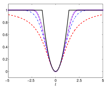
Figure 1: Truncated quadratic penalty in Example 2(i) (black, full) and its smooth approximations $\psi_{s,\delta}(t)$ as defined in Examples 2(ii) (red, dashed), 2(iii) (blue, dash-dot), 2(iv) (green, dot), and 2(v) (magenta, cross), for parameters $\lambda=1$ and $\delta=1$.

2.3 Asymptotic convergence to $\ell_{0}$ criterion

The asymptotic behavior of the considered class of potentials can now be derived by showing the epi-convergence of $F_{\delta}$ to the following block (or group) $\ell_{0}$-penalized objective function:

$$F_{0}\colon{\mathb{x}}\mapsto\Phi({\mathb{H}}{\mathb{x}}-{\mathb{y}})+\lambda\ell_{0}({\mathb{V}}{\mathb{x}}-{\mathb{c}})+\|{\mathb{V}}_{0}{\mathb{x}}\|^{2},$$ (12)

where ${\mathb{V}}=\left[{\mathb{V}}_{1}^{\top}\,|\,\ldots\,|\,{\mathb{V}}_{S}^{\top}\right]^{\top}$, ${\mathb{c}}=\left[{\mathb{c}}_{1}^{\top},\ldots,{\mathb{c}}_{S}^{\top}\right]^{\top}$, and $\ell_{0}$ denotes the so-called ‘block $\ell_{0}$ cost’ [25] defined as

$$(\forall{\mathb{t}}=[{\mathb{t}}_{1}^{\top},\ldots,{\mathb{t}}_{S}^{\top}]^{\top}\in{\mathbb{R}}^{P_{1}+\cdots+P_{S}})\qquad\ell_{0}({\mathb{t}})=\sum_{s=1}^{S}\chi_{{\mathbb{R}}\backslash\left\{0\right\}}(\|{\mathb{t}}_{s}\|),$$ (13)

where, for every $s\in\{1,\ldots,S\}$, ${\mathb{t}}_{s}\in{\mathbb{R}}^{P_{s}}$. When $P_{1}=\ldots=P_{S}=1$, (13) provides the standard expression of the $\ell_{0}$ cost of ${\mathbb{R}}^{S}$.

Proposition 2.

Suppose that Assumptions 1 and 2 hold. Let $(\delta_{n})_{n\in\mathbb{N}}$ be a decreasing sequence of positive real numbers converging to $0$. Then,

1. $\inf F_{\delta_{n}}\to\inf F_{0}$ as $n\to+\infty$.

2. If $(\forall n\in\mathbb{N})$ $\widehat{{\mathb{x}}}_{n}$ is a minimizer of $F_{\delta_{n}}$, then the sequence $(\widehat{{\mathb{x}}}_{n})_{n\in\mathbb{N}}$ is bounded and all its cluster points are minimizers of $F_{0}$.

3. If $F_{0}$ has a unique minimizer $\widetilde{{\mathb{x}}}$, then $\widehat{{\mathb{x}}}_{n}\to\widetilde{{\mathb{x}}}$ as $n\to+\infty$.

Proof.

First, note that, according to Assumption 2(i), for every $n\in\mathbb{N}$, $F_{\delta_{n+1}}\geq F_{\delta_{n}}$. In addition, for every $n\in\mathbb{N}$, $F_{\delta_{n}}$ is a continuous function as a consequence of Assumptions 1(i) and 1(ii). Then it can be deduced from [53, Theorem 7.4(d)] that $(F_{\delta_{n}})_{n\in\mathbb{N}}$ epi-converges to $\sup_{n\in\mathbb{N}}F_{\delta_{n}}$. The latter function is equal to $F_{0}$ by virtue of Assumption 2(ii). In addition, $(F_{\delta_{n}})_{n\in\mathbb{N}}$ is eventually level-bounded as a consequence of [53, Ex. 7.32(a)], the lower bound in (4) and the fact that $\underline{F}\colon{\mathb{x}}\mapsto\Phi({\mathb{H}}{\mathb{x}}-{\mathb{y}})+\|{\mathb{V}}_{0}{\mathb{x}}\|^{2}$ is level-bounded (as shown in the proof of Proposition 1). We complete the proof by noticing that $F_{0}$ is lower semicontinuous and proper, and by applying [53, Theorem 7.33]. ∎

The above proposition guarantees that a minimizer of $F_{0}$ can be well-approximated by choosing a small enough $\delta$. Note that the existence/uniqueness of a minimizer of $F_{0}$ is discussed in the literature on compressed sensing under some specific assumptions [14, 19, 22, 46].

We will now turn our attention to numerical methods allowing us to efficiently solve Problem (1) when all the involved functions are smooth.

3 Proposed optimization method

3.1 Subspace algorithm

A classical strategy to minimize the criterion $F_{\delta}$ consists of building a sequence $({\mathb{x}}_{k})_{k\in\mathbb{N}}$ of ${\mathbb{R}}^{N}$ such that

$$(\forall k\in\mathbb{N})\qquad F_{\delta}({\mathb{x}}_{k+1})\leq F_{\delta}({\mathb{x}}_{k}).$$ (14)

This can be performed by translating the current solution ${\mathb{x}}_{k}$ at each iteration $k\in\mathbb{N}$ along a suitable direction ${\mathb{d}}_{k}\in{\mathbb{R}}^{N}$:

$${\mathb{x}}_{k+1}={\mathb{x}}_{k}+\alpha_{k}{\mathb{d}}_{k},$$ (15)

where $\alpha_{k}>0$ is the step size, and ${\mathb{d}}_{k}$ is a descent direction. When $F_{\delta}$ is differentiable, this direction is chosen such that ${\mathb{g}}_{k}^{\top}{\mathb{d}}_{k}\leq 0$ where ${\mathb{g}}_{k}$ denotes the gradient of $F_{\delta}$ at ${\mathb{x}}_{k}$.

A significant practical improvement regarding the convergence rate is achieved by performing subspace acceleration, i.e. by considering a set of $M$ search directions $\{{\mathb{d}}_{k}^{1},\ldots,{\mathb{d}}_{k}^{M}\}\subset{\mathbb{R}}^{N}$ and by defining the new iteration as

$${\mathb{x}}_{k+1}={\mathb{x}}_{k}+{\mathb{D}}_{k}{\boldsymbol{u}}_{k},$$ (16)

where ${\mathb{D}}_{k}=[{\mathb{d}}_{k}^{1},\ldots,{\mathb{d}}_{k}^{M}]\in{\mathbb{R}}^{N\times M}$ is the search direction matrix and ${\boldsymbol{u}}_{k}\in{\mathbb{R}}^{M}$ is a multivariate step size, which is computed so as to minimize

$$f_{k,\delta}\colon{\boldsymbol{u}}\mapsto F_{\delta}({\mathb{x}}_{k}+{\mathb{D}}_{k}{\boldsymbol{u}}).$$ (17)

The memory gradient subspace algorithm, initially proposed in the late 1960’s by Miele and Cantrell [43], corresponds to:

$$(\forall k\geq 1)\qquad{\mathb{D}}_{k}=[-{\mathb{g}}_{k}\;\left|\right.\;{\mathb{x}}_{k}-{\mathb{x}}_{k-1}].$$ (18)

When the objective function is quadratic, this algorithm is equivalent to the linear conjugate gradient algorithm [15]. More recently, several other subspace algorithms have been proposed, where, at each iteration $k\in{\mathbb{N}}$, ${\mathb{D}}_{k}$ usually includes a descent direction (e.g. gradient, Newton, truncated Newton directions) and a short history of previous directions (see [17, Tab.1] for a general review).

In addition, the subspace scheme (16) was shown to outperform standard descent algorithms such as nonlinear conjugate gradient over a set of PLS minimization problems in [17, 62]. The convergence of Algorithm (16) however requires the design of a proper strategy to determine the step sizes $({\boldsymbol{u}}_{k})_{k\in{\mathbb{N}}}$, which we discuss in the next section.

3.2 Majorize-Minimize step size

At each iteration $k\in{\mathbb{N}}$, the minimization of $f_{k,\delta}$ using the Majorization-Minimization (MM) principle is approximately performed by successive minimizations of tangent majorant functions for $f_{k,\delta}$. Let $q_{k}\colon{\mathbb{R}}^{M}\times{\mathbb{R}}^{M}\to{\mathbb{R}}$ and let ${\boldsymbol{u}}^{\prime}\in{\mathbb{R}}^{M}$. The function $q_{k}(.,{\boldsymbol{u}}^{\prime})$ is said to be a tangent majorant for $f_{k,\delta}$ at ${\boldsymbol{u}}^{\prime}$ if

$$\begin{cases}(\forall{\boldsymbol{u}}\in{\mathbb{R}}^{M})\quad q_{k}({\boldsymbol{u}},{\boldsymbol{u}}^{\prime})\geq f_{k,\delta}({\boldsymbol{u}})\\ q_{k}({\boldsymbol{u}}^{\prime},{\boldsymbol{u}}^{\prime})=f_{k,\delta}({\boldsymbol{u}}^{\prime}).\end{cases}$$ (19)

From this point forward, we assume that $f_{k,\delta}$ is differentiable. Following [17], we propose to employ a convex quadratic tangent majorant function of the form:

$$(\forall{\boldsymbol{u}}\in{\mathbb{R}}^{M})\quad q_{k}({\boldsymbol{u}},{\boldsymbol{u}}^{\prime})=f_{k,\delta}({\boldsymbol{u}}^{\prime})+\nabla f_{k,\delta}({\boldsymbol{u}}^{\prime})^{\top}({\boldsymbol{u}}-{\boldsymbol{u}}^{\prime})+\frac{\raisebox{-1.0pt}{$1$}}{2}({\boldsymbol{u}}-{\boldsymbol{u}}^{\prime})^{\top}{\mathb{B}}_{k,{\boldsymbol{u}}^{\prime}}({\boldsymbol{u}}-{\boldsymbol{u}}^{\prime}),$$ (20)

where $\nabla f_{k,\delta}({\boldsymbol{u}}^{\prime})$ denotes the derivative of $f_{k,\delta}$ at ${\boldsymbol{u}}^{\prime}$, and ${\mathb{B}}_{k,{\boldsymbol{u}}^{\prime}}$ is an $M\times M$ symmetric positive semi-definite matrix that ensures the fulfillment of majorization properties (19). The initial minimization of $f_{k,\delta}$ is replaced by a sequence of easier subproblems, corresponding to the following MM update rule:

$$\left\{\begin{aligned} {\boldsymbol{u}}_{k}^{0}&={\mathbf{0}},\\ \forall j&\in\{1,\,\ldots,\,J\}\\ &\left\lfloor\begin{array}[]{l}{\boldsymbol{u}}_{k}^{j}\in\underset{{\boldsymbol{u}}\in{\mathbb{R}}^{M}}{\operatorname{Argmin}}\;\;q_{k}({\boldsymbol{u}},{\boldsymbol{u}}_{k}^{j-1})\\ \end{array}\right.\end{aligned}\right.$$ (21)

[Note that for $M=1$, this reduces to the scalar MM line search [36].]

3.3 Construction of the majorizing approximation

We now make the following assumption:

Assumption 3.

1. $\Phi$ is differentiable with an $L$-Lipschitzian gradient, i.e.

   $$(\forall{\mathb{z}}\in{\mathbb{R}}^{Q})(\forall{\mathb{z}}^{\prime}\in{\mathbb{R}}^{Q})\,\,\|\nabla\Phi({\mathb{z}})-\nabla\Phi({\mathb{z}}^{\prime})\|\leq L\|{\mathb{z}}-{\mathb{z}}^{\prime}\|.$$ (22)

2. For every $s\in\left\{1,\cdots,S\right\}$, $\psi_{s,\delta}$ is a differentiable function.

3. For every $s\in\left\{1,\cdots,S\right\}$, $\psi_{s,\delta}(\sqrt{.})$ is concave on $[0,+\infty)$.

4. For every $s\in\left\{1,\cdots,S\right\}$, there exists $\overline{\omega_{s}}\in[0,+\infty)$ such that $(\forall t\in(0,+\infty))$ $0\leq\dot{\psi}_{s,\delta}(t)\leq\overline{\omega_{s}}t$ where $\dot{\psi}_{s,\delta}$ is the derivative of $\psi_{s,\delta}$. In addition, $\lim_{\underset{t\neq 0}{t\to 0}}\dot{\psi}_{s,\delta}(t)/t\in{\mathbb{R}}$.

We emphasize the fact that Assumptions 3(ii)-(iv) hold for the $\ell_{2}$-$\ell_{0}$ penalties in Examples 2(ii)-(v). Morever, Tab. 1 presents several examples of functions fulfilling Assumption 3(i).

Function name	$\Phi({\mathb{z}})$	Lipschitz
	${\mathb{z}}=(z_{q})_{1\leq q\leq Q}\in{\mathbb{R}}^{Q}$	constant $L$
Least squares	$\frac{1}{2}{\mathb{z}}^{\top}\Lambda{\mathb{z}}$	$\|\Lambda\|$
	$\Lambda\in{\mathbb{R}}^{Q\times Q}$ symmetric positive semi-definite
$\ell_{2}$- $\ell_{1}$	$\sum_{q=1}^{Q}\phi_{q}(z_{q})$	$\max_{1\leq q\leq Q}(\frac{1}{\sqrt{\rho_{q}}})$
[59]	$(\forall t\in{\mathbb{R}})$ $\phi_{q}(t)=\sqrt{\rho_{q}+t^{2}}$, $\rho_{q}>0$
Huber	$\sum_{q=1}^{Q}\phi_{q}(z_{q})$	$2\max_{1\leq q\leq Q}\rho_{q}$
[31]	$(\forall t\in{\mathbb{R}})$ $\phi_{q}(t)=\begin{cases}\rho_{q}t^{2}&\mbox{if $|t|\leq\nu_{q}$}\\ \rho_{q}\nu_{q}(2|t|-\nu_{q}|)&\mbox{if $|t|>\nu_{q}$}\end{cases}$
	$\nu_{q}>0$, $\rho_{q}>0$
Cauchy	$\sum_{q=1}^{Q}\phi_{q}(z_{q})$	$\max_{1\leq q\leq Q}(\frac{2}{\rho_{q}})$
[2]	$(\forall t\in{\mathbb{R}})$ $\phi_{q}(t)=\ln(\rho_{q}+t^{2})$, $\rho_{q}>0$
Squared distance to	$\frac{1}{2}d_{B}^{2}({\mathb{z}})$	1
a closed convex set $B$ [6]
Smoothed max [7]	$\rho\ln(\sum_{q=1}^{Q}e^{z_{q}/\rho})$, $\rho>0$	$1/\rho$
Inf-convolution	$\inf_{{\mathb{z}}_{1}+{\mathb{z}}_{2}={\mathb{z}}}\Phi_{1}({\mathb{z}}_{1})+\Phi_{2}({\mathb{z}}_{2})$	$\rho$
[6]	$\Phi_{1}\in\Gamma_{0}({\mathbb{R}}^{Q})$, $\Phi_{2}\in\Gamma_{0}({\mathbb{R}}^{Q})$
	$\Phi_{2}$ $\rho$-Lipschitz differentiable, $\rho>0$,
	such that $\lim_{\|{\mathb{z}}\|\to+\infty}\frac{\Phi_{2}({\mathb{z}})}{\|{\mathb{z}}\|}=+\infty$

Table 1: Some examples of functions $\Phi$ with an $L$-Lipschitzian gradient. ($\|\Lambda\|$ denotes the spectral norm of $\Lambda$ and $\Gamma_{0}({\mathbb{R}}^{Q})$ denotes the class of proper lower-semicontinuous convex functions from ${\mathbb{R}}^{Q}$ to $(-\infty,+\infty]$.)

By defining

$$(\forall s\in\{1,\ldots,S\})(\forall t\in{\mathbb{R}})\quad\omega_{s,\delta}(t)=\dot{\psi}_{s,\delta}(t)/t,$$ (23)

(the function $\omega_{s,\delta}$ is extended by continuity at $0$), a tangent majorant can be built as described below:

Lemma 1.

[1] For every ${\mathb{x}}\in{\mathbb{R}}^{N}$, let

$${\mathb{A}}({\mathb{x}})=\mu{\mathb{H}}^{\top}{\mathb{H}}+2{\mathb{V}}_{0}^{\top}{\mathb{V}}_{0}+{\mathb{V}}^{\top}\mathrm{Diag}\left\{{\mathb{b}}({\mathb{x}})\right\}{\mathb{V}},$$ (24)

where $\mu\in[L,+\infty)$ and ${\mathb{b}}({\mathb{x}})=\big{(}b_{i}({\mathb{x}})\big{)}_{1\leq i\leq SP}\in{\mathbb{R}}^{SP}$ with $P=\sum_{s=1}^{S}P_{s}$ is such that

$$(\forall s\in\{1,\ldots,S\})\,(\forall p\in\{1,\ldots,P_{s}\})\quad b_{P_{1}+\cdots+P_{s-1}+p}({\mathb{x}})=\omega_{s,\delta}(\|{\mathb{V}}_{s}{\mathb{x}}-{\mathb{c}}_{s}\|).$$ (25)

Let ${\boldsymbol{u}}^{\prime}\in{\mathbb{R}}^{M}$ and $k\in{\mathbb{N}}$. Then, under Assumption 3, $q_{k}(\cdot,{\boldsymbol{u}}^{\prime})$ with

$${\mathb{B}}_{k,{\boldsymbol{u}}^{\prime}}={\mathb{D}}_{k}^{\top}{\mathb{A}}({\mathb{x}}_{k}+{\mathb{D}}_{k}{\boldsymbol{u}}^{\prime}){\mathb{D}}_{k},$$ (26)

is a convex quadratic tangent majorant of $f_{\delta,k}$ at ${\boldsymbol{u}}^{\prime}$.

Hence, according to (20) and (21), the optimality condition for the choice of the step size in the MM iteration is given by:

$$(\forall k\in{\mathbb{N}})(\forall j\in\{1,\ldots,J\})\quad{\mathb{B}}_{k,{\boldsymbol{u}}_{k}^{j-1}}({\boldsymbol{u}}_{k}^{j}-{\boldsymbol{u}}_{k}^{j-1})+\nabla f_{k,\delta}({\boldsymbol{u}}_{k}^{j-1})=\mathbf{0}.$$ (27)

This yields the explicit step size formula

$${\boldsymbol{u}}_{k}^{j}={\boldsymbol{u}}_{k}^{j-1}-\,{\mathb{B}}_{k,{\boldsymbol{u}}_{k}^{j-1}}^{-1}\,\nabla f_{k,\delta}({\boldsymbol{u}}_{k}^{j-1}),$$ (28)

where ${\mathb{B}}_{k,{\boldsymbol{u}}_{k}^{j-1}}^{-1}$ is the pseudo-inverse of ${\mathb{B}}_{k,{\boldsymbol{u}}_{k}^{j-1}}\in{\mathbb{R}}^{M\times M}$. One of the main advantages of this approach is that the computational cost of the required inversion is low, provided that the number $M$ of search directions remains small. The resulting MM subspace algorithm reads

$$\left\{\begin{array}[]{l}{\mathb{x}}_{0}\in{\mathbb{R}}^{N},\\ \forall k\in{\mathbb{N}}\\ \begin{array}[]{l}\left\lfloor\begin{array}[]{l}{\boldsymbol{u}}_{k}^{0}={\mathbf{0}},\\ \forall j\in\{1,\,\ldots,\,J\}\\ \left\lfloor\begin{array}[]{l}{\mathb{B}}_{k,{\boldsymbol{u}}_{k}^{j-1}}={\mathb{D}}_{k}^{\top}{\mathb{A}}({\mathb{x}}_{k}+{\mathb{D}}_{k}{\boldsymbol{u}}_{k}^{j-1}){\mathb{D}}_{k},\\ {\boldsymbol{u}}_{k}^{j}={\boldsymbol{u}}_{k}^{j-1}-\,{\mathb{B}}_{k,{\boldsymbol{u}}_{k}^{j-1}}^{-1}\,{\mathb{D}}_{k}^{\top}\nabla F_{k,\delta}({\mathb{x}}_{k}+{\mathb{D}}_{k}{\boldsymbol{u}}_{k}^{j-1}),\end{array}\right.\\[2.84526pt] {\mathb{x}}_{k+1}={\mathb{x}}_{k}+{\mathb{D}}_{k}{\boldsymbol{u}}_{k}^{J}.\end{array}\right.\\ \end{array}\end{array}\right.$$ (29)

4 Convergence result

We first provide some preliminary technical lemmas before stating our main convergence result. In the following, for every $k\in\mathbb{N}$ and $j\in\{0,\ldots,J\}$, we define

$${\mathb{x}}_{k}^{j} ={\mathb{x}}_{k}+{\mathb{D}}_{k}{\boldsymbol{u}}_{k}^{j},$$ (30)

$${\mathb{g}}_{k}^{j} =\nabla F_{\delta}({\mathb{x}}_{k}^{j}),$$ (31)

(thus, ${\mathb{x}}_{k}^{J}={\mathb{x}}_{k+1}$ and ${\mathb{g}}_{k}^{J}={\mathb{g}}_{k+1}$). Moreover, we assume that the set of directions $({\mathb{D}}_{k})_{k\in{\mathbb{N}}}$ fulfills the following condition:

Assumption 4.

For every $k\in{\mathbb{N}}$, the matrix of directions ${\mathb{D}}_{k}$ is of size $N\times M$ with $1\leq M\leq N$ and the first subspace direction ${\mathb{d}}_{k}^{1}$ is gradient-related i.e.,

$${\mathb{g}}_{k}^{\top}{\mathb{d}}_{k}^{1} \leq-\gamma_{0}\|{\mathb{g}}_{k}\|^{2},$$ (32)

$$\|{\mathb{d}}_{k}^{1}\| \leq\gamma_{1}\|{\mathb{g}}_{k}\|,$$ (33)

with $\gamma_{0}>0$ and $\gamma_{1}>0$.

As emphasized in [8, Sec.1.2] and [17, Sec.III-D], conditions (32) and (33) hold for a large family of descent directions, such as the steepest descent direction or the truncated Newton direction.

4.1 Preliminary results

Lemma 2.

Under Assumptions 3 and 4, there exists a constant $\nu>0$ such that, for every $k\in{\mathbb{N}}$ and $j\in\{1,\ldots,J\}$, $F_{\delta}({\mathb{x}}_{k})-F_{\delta}({\mathb{x}}_{k}^{j})\geq\frac{\gamma_{0}^{2}}{\gamma_{1}^{2}}\nu^{-1}\|{\mathb{g}}_{k}\|^{2}$.

Proof.

According to Assumption 3(iv) and Eq. (23), for every $s\in\left\{1,\cdots,S\right\}$, $\omega_{s,\delta}$ is upper-bounded on $(0,+\infty)$. Hence, there exists $\nu>0$ such that, for every ${\mathb{x}}\in{\mathbb{R}}^{N}$ and ${\mathb{v}}\in{\mathbb{R}}^{N}$, ${\mathb{v}}^{\top}A({\mathb{x}}){\mathb{v}}\leq\nu\|{\mathb{v}}\|^{2}/2$. The result then follows from [17, Theorem 1]. ∎

Lemma 3.

Under Assumptions 1 and 3, the MM subspace iterates are such that

$$(\forall k\in\mathbb{N})(\forall j\in\{0,\ldots,J-1\})\qquad F_{\delta}({\mathb{x}}_{k}^{j})-F_{\delta}({\mathb{x}}_{k}^{j+1}) \geq\frac{\eta}{2}\|{\mathb{x}}_{k}^{j+1}-{\mathb{x}}_{k}^{j}\|^{2}$$ (34)

where $\eta>0$ is the smallest eigenvalue of $\mu{\mathb{H}}^{\top}{\mathb{H}}+2{\mathb{V}}_{0}^{\top}{\mathb{V}}_{0}$.

Proof.

Let $k\in{\mathbb{N}}$ and $j\in\{0,\ldots,J-1\}$. According to (20) and the definition of ${\boldsymbol{u}}_{k}^{j+1}$,

$$f_{k,\delta}({\boldsymbol{u}}_{k}^{j})-q_{k}({\boldsymbol{u}}_{k}^{j+1},{\boldsymbol{u}}_{k}^{j})=-\frac{1}{2}\nabla f_{k,\delta}({\boldsymbol{u}}_{k}^{j})^{\top}({\boldsymbol{u}}_{k}^{j+1}-{\boldsymbol{u}}_{k}^{j}).$$ (35)

Furthermore, $q_{k}({\boldsymbol{u}}_{k}^{j+1},{\boldsymbol{u}}^{j})\geq f_{k,\delta}({\boldsymbol{u}}_{k}^{j+1})$. Thus,

$$f_{k,\delta}({\boldsymbol{u}}_{k}^{j})-f_{k,\delta}({\boldsymbol{u}}_{k}^{j+1})\geq-\frac{1}{2}\nabla f_{k,\delta}({\boldsymbol{u}}^{j})^{\top}({\boldsymbol{u}}_{k}^{j+1}-{\boldsymbol{u}}_{k}^{j}).$$ (36)

The last inequality also reads

$$F_{\delta}({\mathb{x}}_{k}^{j})-F_{\delta}({\mathb{x}}_{k}^{j+1})\geq-\frac{1}{2}\nabla f_{k,\delta}({\boldsymbol{u}}^{j})^{\top}({\boldsymbol{u}}_{k}^{j+1}-{\boldsymbol{u}}_{k}^{j}).$$ (37)

So, using (26) and (27),

$$F_{\delta}({\mathb{x}}_{k}^{j})-F_{\delta}({\mathb{x}}_{k}^{j+1}) \geq\frac{1}{2}\big{(}{\mathb{D}}_{k}({\boldsymbol{u}}_{k}^{j+1}-{\boldsymbol{u}}_{k}^{j})\big{)}^{\top}{\mathb{A}}({\mathb{x}}_{k}^{j}){\mathb{D}}_{k}({\boldsymbol{u}}_{k}^{j+1}-{\boldsymbol{u}}_{k}^{j})$$ (38)

$$\geq\frac{\eta}{2}\|{\mathb{D}}_{k}({\boldsymbol{u}}_{k}^{j+1}-{\boldsymbol{u}}_{k}^{j})\|^{2}.$$ (39)

In the latter inequality, we make use of the fact that, since $\mathrm{Ker}{\mathb{H}}\cap\mathrm{Ker}{\mathb{V}}_{0}=\left\{{\mathbf{0}}\right\}$, $\eta$ is positive, and

$$(\forall{\mathb{x}}\in{\mathbb{R}}^{N})(\forall{\mathb{v}}\in{\mathbb{R}}^{N})\qquad{\mathb{v}}^{\top}A({\mathb{x}}){\mathb{v}}\geq\eta\|{\mathb{v}}\|^{2}.$$ (40)

∎

Lemma 4.

Under Assumptions 1 and 3, the MM subspace iterates are such that

$$(\forall k\in\mathbb{N})(\forall j\in\{0,\ldots,J-1\})\qquad\eta\|{\mathb{x}}_{k}^{j+1}-{\mathb{x}}_{k}^{j}\| \leq\|{\mathb{g}}_{k}^{j}\|,$$ (41)

where $\eta>0$ is the same constant as in Lemma 3.

Proof.

According to (27), we have, for every $k\in\mathbb{N}$ and $j\in\{0,\ldots,J-1\}$,

$${\mathb{D}}_{k}^{\top}{\mathb{g}}_{k}^{j}+{\mathb{D}}_{k}^{\top}{\mathb{A}}({\mathb{x}}_{k}^{j}){\mathb{D}}_{k}({\boldsymbol{u}}_{k}^{j+1}-{\boldsymbol{u}}_{k}^{j})={\mathbf{0}}.$$ (42)

Hence,

$$\big{(}{\mathb{D}}_{k}({\boldsymbol{u}}_{k}^{j+1}-{\boldsymbol{u}}_{k}^{j})\big{)}^{\top}{\mathb{g}}_{k}^{j}+\big{(}{\mathb{D}}_{k}({\boldsymbol{u}}_{k}^{j+1}-{\boldsymbol{u}}_{k}^{j})\big{)}^{\top}{\mathb{A}}({\mathb{x}}_{k}){\mathb{D}}_{k}({\boldsymbol{u}}_{k}^{j+1}-{\boldsymbol{u}}_{k}^{j})={\mathbf{0}}.$$ (43)

By using (40), (43) leads to

$$-\big{(}{\mathb{D}}_{k}({\boldsymbol{u}}_{k}^{j+1}-{\boldsymbol{u}}_{k}^{j})\big{)}^{\top}{\mathb{g}}_{k}^{j}\geq\eta\|{\mathb{D}}_{k}({\boldsymbol{u}}_{k}^{j+1}-{\boldsymbol{u}}_{k}^{j})\|^{2}.$$ (44)

In addition, the Cauchy-Schwarz inequality leads to

$$-\big{(}{\mathb{D}}_{k}({\boldsymbol{u}}_{k}^{j+1}-{\boldsymbol{u}}_{k}^{j})\big{)}^{\top}{\mathb{g}}_{k}^{j}\leq\|{\mathb{g}}_{k}^{j}\|\|{\mathb{D}}_{k}({\boldsymbol{u}}_{k}^{j+1}-{\boldsymbol{u}}_{k}^{j})\|.$$ (45)

Thus, the latter two inequalities yield:

$$\eta\|{\mathb{D}}_{k}({\boldsymbol{u}}_{k}^{j+1}-{\boldsymbol{u}}_{k}^{j})\|^{2}\leq\|{\mathb{g}}_{k}^{j}\|\|{\mathb{D}}_{k}({\boldsymbol{u}}_{k}^{j+1}-{\boldsymbol{u}}_{k}^{j})\|.$$ (46)

Substituting with (30), we obtain the desired result. ∎

4.2 Convergence theorem

Based on the two previous lemmas, classical results in the optimization literature [48] may allow us to deduce the convergence of the sequence $({\mathb{x}}_{k})_{k\in\mathbb{N}}$ generated by the MM subspace algorithm, but these results require restrictive conditions on the critical points of the objective function $F_{\delta}$. We propose here a more general approach based on recent results in nonconvex optimization [3, 4, 5]. We first recall the following definition from [40]:

Definition 1.

A differentiable function $G\colon{\mathbb{R}}^{N}\to{\mathbb{R}}$ is said to satisfy the Kurdyka-Łojasiewicz inequality if, for every $\widetilde{{\mathb{x}}}\in{\mathbb{R}}^{N}$ and every bounded neighborhood $E$ of $\widetilde{{\mathb{x}}}$, there exist three constants $\kappa>0$, $\zeta>0$ and $\theta\in[0,1)$ such that

$$\|\nabla G({\mathb{x}})\|\geq\kappa|G({\mathb{x}})-G(\widetilde{{\mathb{x}}})|^{\theta},$$ (47)

for every ${\mathb{x}}\in E$ such that $|G({\mathb{x}})-G(\widetilde{{\mathb{x}}})|<\zeta$.

The interesting point is that this inequality is satisfied for a wide class of functions. In particular, it holds for real analytic functions, semi-algebraic functions as well as many others [11, 12, 35, 40]. Recall that a [function] $G\colon{\mathbb{R}}^{N}\to{\mathbb{R}}$ is semi-algebraic if its graph $\{({\mathb{x}},\eta)\in{\mathbb{R}}^{N}\times{\mathbb{R}}\mid\eta=G({\mathb{x}})\}$ is a semi-algebraic set, i.e. it can be expressed as a finite union of subsets of ${\mathbb{R}}^{N}\times{\mathbb{R}}$ defined by a finite number of polynomial inequalities. The semi-algebraicity property is stable under various operations (sum, product, inversion, composition,…). Examples of semi-algebraic functions include ${\mathb{x}}\mapsto\|{\mathb{H}}{\mathb{x}}-{\mathb{y}}\|^{2}$, $\Psi_{\delta}$ when the functions $(\psi_{s,\delta})_{1\leq s\leq S}$ are given by Example 2(ii) or 2(v), the squared distance to a closed convex semi-algebraic set. In turn, examples of real-analytic functions include ${\mathb{x}}\mapsto\|{\mathb{H}}{\mathb{x}}-{\mathb{y}}\|^{2}$ and $\Psi_{\delta}$ when the functions $(\psi_{s,\delta})_{1\leq s\leq S}$ are given by Examples 2(ii)-2(iv). Note that a more general local version of inequality (47) can also be found in the literature [12].

Let us now state our main convergence result:

Theorem 3.

Assume that $F_{\delta}$ satisfies the Kurdyka-Łojasiewicz inequality. Under Assumptions 1, 3 and 4, the MM subspace algorithm given by (29) generates a sequence $({\mathb{x}}_{k})_{k\in\mathbb{N}}$ converging to a critical point $\widetilde{{\mathb{x}}}$ of $F_{\delta}$. Moreover, this sequence is of finite length, in the sense that

$$\sum_{k=0}^{+\infty}\|{\mathb{x}}_{k+1}-{\mathb{x}}_{k}\|<+\infty.$$ (48)

Proof.

As $(F_{\delta}({\mathb{x}}_{k}))_{k\in\mathbb{N}}$ is a decreasing sequence and $\operatorname{lev}_{\leq F_{\delta}({\mathb{x}}_{0})}=\left\{{\mathb{x}}\in{\mathbb{R}}^{N}|F_{\delta}({\mathb{x}})\leq F_{\delta}({\mathb{x}}_{0})\right\}$ is a bounded set (by virtue of Proposition 1(i)), the sequence $({\mathb{x}}_{k})_{k\in\mathbb{N}}$ belongs to a compact subset $E$ of ${\mathbb{R}}^{N}$. Hence, there exists a subsequence $({\mathb{x}}_{k_{i}})_{i\in\mathbb{N}}$ of $({\mathb{x}}_{k})_{k\in\mathbb{N}}$ converging to a vector $\widetilde{{\mathb{x}}}$ of ${\mathbb{R}}^{N}$. Besides, since $F_{\delta}$ is a continuous function, $(F_{\delta}({\mathb{x}}_{k_{i}}))_{i\in\mathbb{N}}$ converges to $F_{\delta}(\widetilde{{\mathb{x}}})$. As $(F_{\delta}({\mathb{x}}_{k}))_{k\in\mathbb{N}}$ is decreasing, and Proposition 1(i) shows that it is [bounded below], we deduce that $(F_{\delta}({\mathb{x}}_{k})-F_{\delta}(\widetilde{{\mathb{x}}}))_{k\in\mathbb{N}}$ is a nonnegative sequence converging to 0.

Now, by invoking Lemma 2 (with $j=J$), we have that, for every $k\in\mathbb{N}$,

$$\frac{\gamma_{0}^{2}}{\gamma_{1}^{2}}\nu^{-1}\|{\mathb{g}}_{k}\|^{2} \leq F_{\delta}({\mathb{x}}_{k})-F_{\delta}({\mathb{x}}_{k+1})=F_{\delta}({\mathb{x}}_{k})-F_{\delta}(\widetilde{{\mathb{x}}})-\big{(}F_{\delta}({\mathb{x}}_{k+1})-F_{\delta}(\widetilde{{\mathb{x}}})\big{)}.$$ (49)

According to the Łojasiewicz property, there exist constants $\kappa>0$, $\zeta>0$ and $\theta\in[0,1)$ such that

$$\|\nabla F_{\delta}({\mathb{x}})\|\geq\kappa|F_{\delta}({\mathb{x}})-F_{\delta}(\widetilde{{\mathb{x}}})|^{\theta},$$ (50)

for every ${\mathb{x}}\in E$ such that $|F_{\delta}({\mathb{x}})-F_{\delta}(\widetilde{{\mathb{x}}})|<\zeta$. We now apply to the convex function $\varphi\colon[0,+\infty)\to[0,+\infty)\colon u\mapsto u^{1/(1-\theta)}$ the following gradient inequality

$$(\forall(u,v)\in[0,+\infty)^{2})\qquad\varphi(v)\geq\varphi(u)+\dot{\varphi}(u)(v-u)$$ (51)

which, after a change of variables, can be rewritten as

$$(\forall(u,v)\in[0,+\infty)^{2})\qquad u-v\leq(1-\theta)^{-1}u^{\theta}(u^{1-\theta}-v^{1-\theta}).$$ (52)

Combining the latter inequality with (49) leads to

$$F_{\delta}({\mathb{x}}_{k})-F_{\delta}(\widetilde{{\mathb{x}}})-\big{(}F_{\delta}({\mathb{x}}_{k+1})-F_{\delta}(\widetilde{{\mathb{x}}})\big{)} \leq(1-\theta)^{-1}(F_{\delta}({\mathb{x}}_{k})-F_{\delta}(\widetilde{{\mathb{x}}}))^{\theta}\Delta_{k}$$ (53)

where

$$\Delta_{k}=\big{(}F_{\delta}({\mathb{x}}_{k})-F_{\delta}(\widetilde{{\mathb{x}}})\big{)}^{1-\theta}-\big{(}F_{\delta}({\mathb{x}}_{k+1})-F_{\delta}(\widetilde{{\mathb{x}}})\big{)}^{1-\theta}.$$ (54)

Thus,

$$\|{\mathb{g}}_{k}\|^{2} \leq\frac{\gamma_{1}^{2}}{\gamma_{0}^{2}}\nu(1-\theta)^{-1}(F_{\delta}({\mathb{x}}_{k})-F_{\delta}(\widetilde{{\mathb{x}}}))^{\theta}\Delta_{k}.$$ (55)

Since $(F_{\delta}({\mathb{x}}_{k}))_{k\in\mathbb{N}}$ converges to $F_{\delta}(\widetilde{{\mathb{x}}})$, there exists $k^{*}\in{\mathbb{N}}$, such that, for every $k\geq k^{*}$, $0\leq F_{\delta}({\mathb{x}}_{k})-F_{\delta}(\widetilde{{\mathb{x}}})<\zeta$. By applying the Łojasiewicz inequality,

$$(\forall k\geq k^{*})\qquad\|{\mathb{g}}_{k}\|^{2} \leq\frac{\gamma_{1}^{2}}{\gamma_{0}^{2}}\nu\kappa^{-1}(1-\theta)^{-1}\|{\mathb{g}}_{k}\|\Delta_{k}.$$ (56)

This allows us to deduce that

$$\sum_{k=k^{*}}^{+\infty}\|{\mathb{g}}_{k}\|\leq\frac{\gamma_{1}^{2}}{\gamma_{0}^{2}}\nu\kappa^{-1}(1-\theta)^{-1}\big{(}F_{\delta}({\mathb{x}}_{k^{*}})-F_{\delta}(\widetilde{{\mathb{x}}})\big{)}^{1-\theta}.$$ (57)

Furthermore, according to (30),

$$\frac{\eta}{2}\|{\mathb{x}}_{k+1}-{\mathb{x}}_{k}\|^{2}=\frac{\eta}{2}\Big{\|}\sum_{j=0}^{J-1}({\mathb{x}}_{k}^{j+1}-{\mathb{x}}_{k}^{j})\Big{\|}^{2}$$ (58)

which, by using Lemma 3 and the convexity of the squared norm, yields for every $k\in\mathbb{N}$,

$$\frac{\eta}{2}\|{\mathb{x}}_{k+1}-{\mathb{x}}_{k}\|^{2} \leq\frac{\eta J}{2}\sum_{j=0}^{J-1}\|{\mathb{x}}_{k}^{j+1}-{\mathb{x}}_{k}^{j}\|^{2}$$

$$\leq J\sum_{j=0}^{J-1}F_{\delta}({\mathb{x}}_{k}^{j})-F_{\delta}({\mathb{x}}_{k}^{j+1})=J\big{(}F_{\delta}({\mathb{x}}_{k})-F_{\delta}({\mathb{x}}_{k+1})\big{)}.$$ (59)

By proceeding similarly to the derivation of (56), we obtain: for every $k\geq k^{*}$,

$$\frac{\eta}{2}\|{\mathb{x}}_{k+1}-{\mathb{x}}_{k}\|^{2}\leq J(1-\theta)^{-1}\big{(}F_{\delta}({\mathb{x}}_{k})-F_{\delta}(\widetilde{{\mathb{x}}})\big{)}^{\theta}\Delta_{k}\leq J\kappa^{-1}(1-\theta)^{-1}\|{\mathb{g}}_{k}\|\Delta_{k}.$$ (60)

By using the fact that, for every $(u,v)\in[0,+\infty)^{2}$, $(uv)^{1/2}\leq u+\frac{v}{4}$, and taking $u=J\eta^{-1}\kappa^{-1}(1-\theta)^{-1}\Delta_{k}$ and $v=2\|{\mathb{g}}_{k}\|$, (60) leads to

$$\|{\mathb{x}}_{k+1}-{\mathb{x}}_{k}\|\leq J\eta^{-1}\kappa^{-1}(1-\theta)^{-1}\Delta_{k}+\frac{1}{2}\|{\mathb{g}}_{k}\|.$$ (61)

By summing now over $k$ and using (54) and (57), we finally obtain

$$\sum_{k=k^{*}}^{+\infty}\|{\mathb{x}}_{k+1}-{\mathb{x}}_{k}\|\leq\kappa^{-1}(1-\theta)^{-1}(J\eta^{-1}+\frac{\gamma_{1}^{2}}{\gamma_{0}^{2}}\frac{\nu}{2})\big{(}F_{\delta}({\mathb{x}}_{k^{*}})-F_{\delta}(\widetilde{{\mathb{x}}})\big{)}^{1-\theta}.$$ (62)

This gives us the desired finite length property. In addition, since this condition implies that $({\mathb{x}}_{k})_{k\in\mathbb{N}}$ is a Cauchy sequence, it converges towards a single point, which is necessarily $\widetilde{{\mathb{x}}}$. Finally, due to the continuity of $F_{\delta}$ and Lemma 2, $({\mathb{g}}_{k})_{k\in{\mathbb{N}}}$ converges to zero. As $(x_{k},F_{\delta}(x_{k}))\to(\widetilde{{\mathb{x}}},F_{\delta}(\widetilde{{\mathb{x}}}))$, the closedness property of the gradient implies that $\nabla F_{\delta}(\widetilde{{\mathb{x}}})={\mathbf{0}}$, i.e. $\widetilde{{\mathb{x}}}$ must be a critical point of $F_{\delta}$.

∎

Note that the inexact gradient methods that are studied in [5] [are distinct from the subspace algorithms we consider].

5 Simulation results

The aim of this section is to illustrate and analyze the performance of the proposed algorithm in the context of Problem (1). [We also show the nonconvex penalization functions in Example 2 to be appropriate for image processing applications.] To this end, four image processing problems are considered, namely denoising, segmentation, deblurring and tomographic reconstruction. For each of them, the produced image $\widehat{{\mathb{x}}}\in{\mathbb{R}}^{N}$ is defined as a minimizer of the function $F_{\delta}$, where $\Phi$, ${\mathb{H}}$, ${\mathb{y}}$ and ${\mathb{V}}$ depend on the considered application. For the elastic net regularization term, we choose ${\mathb{V}}_{0}=\tau{\mathb{I}}$, $\tau\geq 0$. For deblurring and tomographic applications, the linear operator ${\mathb{H}}$ is not necessarily injective. Thus, we set $\tau$ equal to a small positive value in order to fulfill Assumption 1(iii). In the two other cases, $\tau$ is set to zero.

For every $s\in\{1,\ldots,S\}$, we have set ${\mathb{c}}_{s}={\mathbf{0}}$. For the potential function $\psi_{s,\delta}$, we have tested the smooth convex $\ell_{2}-\ell_{1}$ function $\psi_{s,\delta}\colon t\mapsto\lambda(\sqrt{1+{t^{2}/\delta^{2}}}-1)$ with $\lambda>0$ (SC) and the smooth nonconvex functions in Example 2(ii) (SNC(ii)), Example 2(iii) (SNC(iii)), Example 2(iv) (SNC(iv)) and Example 2(v) (SNC(v)). Moreover, in the denoising and segmentation examples, we provide optimization results for four state-of-the-art combinatorial optimization algorithms, namely the $\alpha$-expansion [13] ($\alpha$-EXP), Quantized-Convex Move Splitting [33] (QCSM), Tree-Reweighted (TRW) [34] and Belief Propagation (BP) [26] algorithms, for which the nonsmooth nonconvex truncated quadratic function in Example 2(i) (NSNC) is considered. When the linear degradation operator is not the identity matrix, we do not provide any comparison with the combinatorial algorithms. Indeed, although a few algorithms [51, 50] are applicable to inverse problems involving a linear degradation operator, these methods are well-founded only for a sparse convolution operator ${\mathb{H}}$. Moreover, they rely on an adaptation of the graph cut $\alpha$-expansion algorithm, which is shown in our segmentation and denoising examples to be outperformed by our approach.

The computation of the proposed MM subspace algorithm requires specifying the direction set ${\mathb{D}}_{k}$, for every $k\in{\mathbb{N}}$, and the number of MM sub-iterations $J$. [First, the memory-gradient direction matrices,]

$$(\forall k\geq m)\qquad{\mathb{D}}_{k}=[-{\mathb{g}}_{k}\;\left|\right.\;{\mathb{x}}_{k}-{\mathb{x}}_{k-1}\;\left|\right.\;\cdots\;\left|\right.\;{\mathb{x}}_{k-m+1}-{\mathb{x}}_{k-m}]\in{\mathbb{R}}^{N\times(m+1)},$$ (63)

[with memory parameter $m\geq 0$, is considered. Moreover, in all our experiments, we set $J=1$. This choice was observed to yield the best results in terms of convergence profile in the context of MM-based step size computation [17, 36]. In the following, we compare our proposed subspace algorithm, denoted hereafter by 3MG-$m$ (for Majorize-Minimize Memory Gradient) with three other iterative first order descent methods. The methods we compare against are namely the nonlinear conjugate gradient (NLCG) algorithm [29], the L-BFGS algorithm [39] with the memory parameter set to $3$, and the fast version of half quadratic (HQ) algorithm [1].] For each descent algorithm, the MM scalar line search with $J=1$ is employed for the computation of the step size. In the case of HQ, the inner optimization problems are solved partially with conjugate gradient iterations. [Note that this algorithm has been previously studied in the context of nonconvex regularization functions in [20, 52].] In order to [limit the influence of possible local minima in the nonconvex case], the result of $10$ iterations of convex minimization using an $\ell_{2}-\ell_{1}$ penalty is employed as an initialization. In the convex case, minimization is started with the constant null image. The computational complexity is evaluated in terms of iteration number and computational time in seconds necessary to achieve the global stopping rule $\|{\mathb{g}}_{k}\|/\sqrt{N}<10^{-4}$. C++ codes were compiled with the Intel compiler icpc (version 12.1.0) and were run on an Intel(R) Xeon(R) CPU X5570 at 2.93GHz, in a single thread.

5.1 Image denoising

The first problem considered in this section corresponds to the recovery of an image $\overline{{\mathb{x}}}$ from noisy observations ${\mathb{u}}=\overline{{\mathb{x}}}+{\mathb{w}}$ where ${\mathb{w}}$ is a realization of a zero-mean white Gaussian noise. The vector $\overline{{\mathb{x}}}$ here corresponds to the Word image of size $N=128\times 128$ pixels. The variance of the noise was adjusted to correspond to a signal-to-noise ratio (SNR) of $15$ dB (Figure 3). The recovery of the original image is performed by solving (1) where $Q=2N$,

$${\mathb{H}}=\left[\begin{array}[]{c}{\mathb{I}}\\ {\mathb{I}}\end{array}\right]\qquad{\mathb{y}}=\left[\begin{array}[]{c}{\mathb{u}}\\ {\mathbf{0}}\end{array}\right],$$ (64)

and

$$(\forall{\mathb{z}}=(z_{q})_{1\leq q\leq 2N})\qquad\Phi({\mathb{z}})=\frac{1}{2}\left(\sum_{q=1}^{N}z_{q}^{2}+\beta\sum_{q=N+1}^{2N}d_{B}^{2}(z_{q})\right),$$ (65)

where $d_{B}$ denotes the distance to the closed convex interval $B=[0,255]$ and $\beta>0$ is a weighting factor. Then, $\Phi$ is Lipschitz differentiable with Lipschitz constant $L=\max(1,\beta)$. In the sequel, we choose $\beta=1$ so that we have $L=1$. Moreover, the penalization term (3) is used, with $\tau=0$ and an anisotropic penalization on neighboring pixels i.e., $S=2N$, and for every $s\in\{1,\ldots,N\}$ (resp. $s\in\{N+1,\ldots,2N\}$), $P_{s}=1$ and ${\mathb{V}}_{s}$ corresponds to a horizontal (resp. vertical) gradient operator. This anisotropic term is chosen so as to compare more fairly our approach with the combinatorial methods.

Parameters $\lambda$ and $\delta$ were chosen to maximize the SNR between the original image and its reconstructed version. In Figure 3, the reconstructed images are displayed and the corresponding SNR and MSSIM [60] values are provided. Morever, the absolute values of the reconstruction errors $\widehat{{\mathb{x}}}-\overline{{\mathb{x}}}$ are illustrated. It should be noticed that the nonconvex regularization strategy with penalty function SNC(ii) leads to the best results in terms of reconstruction quality.

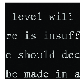
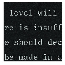
$(a)$	$(b)$

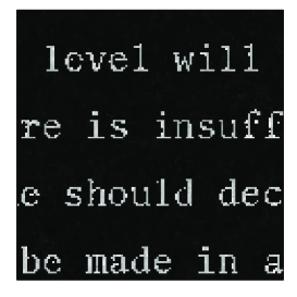
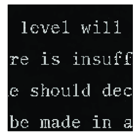
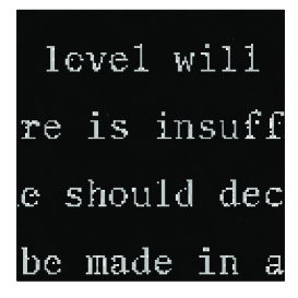
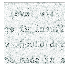
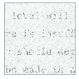
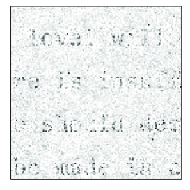
Figure 2: $(a)$ Original image with $128\times 128$ pixels and $(b)$ noisy image with SNR $=15$ dB, MSSIM $=0.66$, and noise standard deviation equal to $10$.

$(a)$	$(b)$	$(c)$

Figure 3: $(a)$ Denoising results and absolute reconstruction error with SC penalty using 3MG, $\lambda=0.3$, $\delta=0.07$, SNR = $20.41$ dB, MSSIM = $0.89$, $(b)$ with NSNC penalty using TRW, $\lambda=350$, $\delta=3.5$, SNR = $22.8$ dB, MSSIM = $0.93$, and $(c)$ with SNC(ii) penalty using 3MG, $\lambda=280$, $\delta=7.25$, SNR = $22.74$ dB, MSSIM = $0.92$.

5.1.1 Influence of memory size

[ We first analyze the effect of the memory size $m$ on the performance of our algorithm. We recall that the detailed performance analysis of 3MG algorithm with respect to the size of the memory was provided in [17], but it was restricted to the convex case. The results in Tab. 2 illustrate that the choice where memory equals one, which corresponds to a subspace with size $2$, leads to the best results in terms of computational time. Hence, our experiments confirm the conclusions drawn in [17] for the convex case. Consequently, $m=1$, i.e.] ${\mathb{D}}_{k}=[-{\mathb{g}}_{k}\;\left|\right.\;{\mathb{x}}_{k}-{\mathb{x}}_{k-1}]$ for all $k\geq 1$ [was retained for the remaining experiments presented in the paper, and the shorter notation 3MG is employed for denoting the 3MG-$1$ algorithm. ]

Penalty function $(\lambda,\delta)$	Algorithm	Iteration	Time	$F_{\delta}$	SNR (dB)
SNC(ii) $(280,7.25)$	3MG-$0$	$998$	$1.08$	$1.54\cdot 10^{6}$	$22.74$
	3MG-$1$	$270$	$0.35$	$1.54\cdot 10^{6}$	$22.74$
	3MG-$2$	$247$	$0.38$	$1.54\cdot 10^{6}$	$22.74$
	3MG-$3$	$248$	$0.44$	$1.54\cdot 10^{6}$	$22.74$
	3MG-$4$	$243$	$0.51$	$1.54\cdot 10^{6}$	$22.74$
	3MG-$5$	$239$	$0.59$	$1.54\cdot 10^{6}$	$22.74$
SNC(iii) $(301,8.76)$	3MG-$0$	$536$	$0.66$	$1.59\cdot 10^{6}$	$22.55$
	3MG-$1$	$101$	$0.21$	$1.59\cdot 10^{6}$	$22.55$
	3MG-$2$	$159$	$0.28$	$1.59\cdot 10^{6}$	$22.55$
	3MG-$3$	$158$	$0.32$	$1.59\cdot 10^{6}$	$22.55$
	3MG-$4$	$156$	$0.36$	$1.59\cdot 10^{6}$	$22.55$
	3MG-$5$	$155$	$0.41$	$1.59\cdot 10^{6}$	$22.55$
SNC(iv) $(381,10)$	3MG-$0$	$287$	$0.61$	$1.8\cdot 10^{6}$	$22.47$
	3MG-$1$	$69$	$0.16$	$1.8\cdot 10^{6}$	$22.47$
	3MG-$2$	$70$	$0.19$	$1.8\cdot 10^{6}$	$22.47$
	3MG-$3$	$67$	$0.21$	$1.8\cdot 10^{6}$	$22.47$
	3MG-$4$	$66$	$0.22$	$1.8\cdot 10^{6}$	$22.47$
	3MG-$5$	$67$	$0.28$	$1.8\cdot 10^{6}$	$22.47$
SNC(v) $(386,9)$	3MG-$0$	$202$	$0.42$	$1.8\cdot 10^{6}$	$22.48$
	3MG-$1$	$49$	$0.11$	$1.8\cdot 10^{6}$	$22.48$
	3MG-$2$	$51$	$0.13$	$1.8\cdot 10^{6}$	$22.48$
	3MG-$3$	$51$	$0.16$	$1.8\cdot 10^{6}$	$22.48$
	3MG-$4$	$52$	$0.17$	$1.8\cdot 10^{6}$	$22.48$
	3MG-$5$	$52$	$0.21$	$1.8\cdot 10^{6}$	$22.48$

Table 2: Denoising problem with word image. Influence of memory parameter $m$ in 3MG algorithm.

5.1.2 Comparison with NLCG algorithm

[ The NLCG algorithm is based on the following iterations:

$$(\forall k\geq 1)\qquad{\mathb{x}}_{k+1}={\mathb{x}}_{k}+\alpha_{k}(-{\mathb{g}}_{k}+\beta_{k}({\mathb{x}}_{k}-{\mathb{x}}_{k-1})),$$ (66)

where $\alpha_{k}>0$ is the step size and $\beta_{k}\in{\mathbb{R}}$ is the conjugacy parameter. Tab. 3 summarizes the performances of NLCG for five different conjugacy strategies described in [29]. Contrary to the convex case, in the nonconvex case the conjugacy formula has a major influence on the convergence speed (see Tab. 3 results related to NLCG in rows 1-6 and 7-30). In particular the conjugacy strategies FR and DY do not appear well-adapted to the nonconvex problems. On the other hand, the HS, LS and PRP+ conjugacy parameters yield good numerical performance. Thus, they have been selected for the numerical experiments in the following. For comparison, we include in Tab. 3 the results of 3MG for $m=1$. Although the superiority of 3MG versus NLCG is not established theoretically, these experimental results are very promising. They show that 3MG algorithm is faster than the considered non-linear conjugate gradient algorithms. ]

Penalty function $(\lambda,\delta)$	Algorithm	Iteration	Time	$F_{\delta}$	SNR (dB)
SC $(0.3,0.07)$	NLCG-HS	$138$	$0.84$	$2.7\cdot 10^{6}$	$20.41$
	NLCG-FR	$305$	$1.86$	$2.7\cdot 10^{6}$	$20.41$
	NLCG-PRP+	$143$	$0.87$	$2.7\cdot 10^{6}$	$20.41$
	NLCG-LS	$158$	$0.96$	$2.7\cdot 10^{6}$	$20.41$
	NLCG-DY	$223$	$1.35$	$2.7\cdot 10^{6}$	$20.41$
	3MG	$122$	$0.22$	$2.7\cdot 10^{6}$	$20.41$
SNC(ii) $(280,7.25)$	NLCG-HS	$1250$	$2.34$	$1.54\cdot 10^{6}$	$22.74$
	NLCG-FR	$>10000$	$-$	$-$	$-$
	NLCG-PRP+	$292$	$0.55$	$1.54\cdot 10^{6}$	$22.74$
	NLCG-LS	$320$	$0.79$	$1.54\cdot 10^{6}$	$22.74$
	NLCG-DY	$>10000$	$-$	$-$	$-$
	3MG	$270$	$0.35$	$1.54\cdot 10^{6}$	$22.74$
SNC(iii) $(301,8.76)$	NLCG-HS	$112$	$0.26$	$1.59\cdot 10^{6}$	$22.55$
	NLCG-FR	$>10000$	$-$	$-$	$-$
	NLCG-PRP+	$179$	$0.42$	$1.59\cdot 10^{6}$	$22.55$
	NLCG-LS	$210$	$0.54$	$1.59\cdot 10^{6}$	$22.55$
	NLCG-DY	$>10000$	$-$	$-$	$-$
	3MG	$101$	$0.21$	$1.59\cdot 10^{6}$	$22.55$
SNC(iv) $(381,10)$	NLCG-HS	$102$	$1.1$	$1.8\cdot 10^{6}$	$22.47$
	NLCG-FR	$3289$	$36.3$	$1.8\cdot 10^{6}$	$22.47$
	NLCG-PRP+	$79$	$0.9$	$1.8\cdot 10^{6}$	$22.47$
	NLCG-LS	$90$	$1$	$1.8\cdot 10^{6}$	$22.47$
	NLCG-DY	$3342$	$36.8$	$1.8\cdot 10^{6}$	$22.47$
	3MG	$69$	$0.16$	$1.8\cdot 10^{6}$	$22.47$
SNC(v) $(386,9)$	NLCG-HS	$52$	$0.15$	$1.8\cdot 10^{6}$	$22.48$
	NLCG-FR	$>10000$	$-$	$-$	$-$
	NLCG-PRP+	$55$	$0.16$	$1.8\cdot 10^{6}$	$22.48$
	NLCG-LS	$56$	$0.16$	$1.8\cdot 10^{6}$	$22.48$
	NLCG-DY	$>10000$	$-$	$-$	$-$
	3MG	$49$	$0.11$	$1.8\cdot 10^{6}$	$22.48$

Table 3: Denoising problem with word image. Influence of conjugacy parameter $\beta_{k}$ in NLCG algorithm.

5.1.3 Summary

[ We summarize the results by comparing the performance of continuous and discrete algorithms with SC, SNC and NSNC potential functions (see Tab. 4). One can observe that the considered discrete optimization algorithms lead to a SNR which is very similar to that obtained with smooth nonconvex regularization. However, they are more demanding in terms of computational time than 3MG. Thus, we can conclude that the 3MG algorithm behaves well in comparison with the considered continuous and discrete algorithms. ]

Penalty function $(\lambda,\delta)$	Algorithm	Iteration	Time	$F_{\delta}$	SNR (dB)
SC $(0.3,0.07)$	3MG	$122$	$0.22$	$2.7\cdot 10^{6}$	$20.41$
	[NLCG-HS]	$138$	$0.35$	$2.7\cdot 10^{6}$	$20.41$
	[NLCG-PRP+]	[$143$]	[$0.37$]	[$2.7\cdot 10^{6}$]	[$20.41$]
	[NLCG-LS]	[$158$]	[$0.96$]	[$2.7\cdot 10^{6}$]	[$20.41$]
	L-BFGS	$209$	$0.73$	$2.7\cdot 10^{6}$	$20.41$
	HQ	$670$	$3.03$	$2.7\cdot 10^{6}$	$20.41$
SNC(ii) $(280,7.25)$	3MG	$270$	$0.35$	$1.54\cdot 10^{6}$	$22.74$
	[NLCG-HS]	$1250$	$2.34$	$1.54\cdot 10^{6}$	$22.74$
	[NLCG-PRP+]	[$292$]	[$0.55$]	[$1.54\cdot 10^{6}$]	[$22.74$]
	[NLCG-LS]	[$320$]	[$0.79$]	[$1.54\cdot 10^{6}$]	[$22.74$]
	L-BFGS	$332$	$0.96$	$1.54\cdot 10^{6}$	$22.73$
	HQ	$1025$	$3.84$	$1.54\cdot 10^{6}$	$22.74$
SNC(iii) $(301,8.76)$	3MG	$101$	$0.21$	$1.59\cdot 10^{6}$	$22.55$
	[NLCG-HS]	$112$	$0.26$	$1.59\cdot 10^{6}$	$22.55$
	[NLCG-PRP+]	[$179$]	[$0.42$]	[$1.59\cdot 10^{6}$]	[$22.55$]
	[NLCG-LS]	[$210$]	[$0.54$]	[$1.59\cdot 10^{6}$]	[$22.55$]
	L-BFGS	$351$	$1.08$	$1.59\cdot 10^{6}$	$22.55$
	HQ	$604$	$2.53$	$1.59\cdot 10^{6}$	$22.54$
SNC(iv) $(381,10)$	3MG	$69$	$0.16$	$1.8\cdot 10^{6}$	$22.47$
	[NLCG-HS]	$102$	$0.27$	$1.8\cdot 10^{6}$	$22.47$
	[NLCG-PRP+]	[$79$]	[$0.21$]	[$1.8\cdot 10^{6}$]	[$22.47$]
	[NLCG-LS]	[$90$]	[$1$]	[$1.8\cdot 10^{6}$]	[$22.47$]
	L-BFGS	$94$	$0.32$	$1.8\cdot 10^{6}$	$22.46$
	HQ	$287$	$1.36$	$1.8\cdot 10^{6}$	$22.47$
SNC(v) $(386,9)$	3MG	$49$	$0.11$	$1.8\cdot 10^{6}$	$22.48$
	[NLCG-HS]	$52$	$0.15$	$1.8\cdot 10^{6}$	$22.48$
	[NLCG-PRP+]	[$55$]	[$0.16$]	[$1.8\cdot 10^{6}$]	[$22.48$]
	[NLCG-LS]	[$56$]	[$0.16$]	[$1.8\cdot 10^{6}$]	[$22.48$]
	L-BFGS	$80$	$0.25$	$1.8\cdot 10^{6}$	$22.48$
	HQ	$202$	$1.1$	$1.8\cdot 10^{6}$	$22.48$
NSNC $(350,3.5)$	$\alpha$-EXP	$4$	$4.67$	$1.31\cdot 10^{6}$	$22.69$
	QCSM	$2$	$1.25$	$1.31\cdot 10^{6}$	$22.60$
	TRW	$5$	$1.65$	$1.31\cdot 10^{6}$	$22.80$
	BP	$18$	$5.33$	$1.31\cdot 10^{6}$	$22.73$

Table 4: Results for the denoising problem.

5.2 Image segmentation

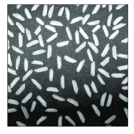
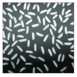
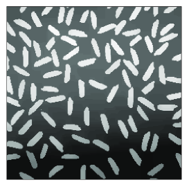
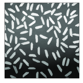
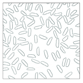
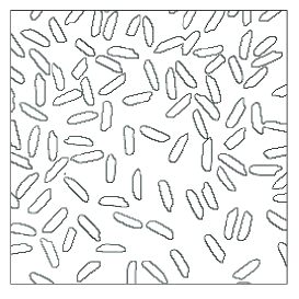
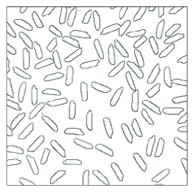
Figure 4: Initial gray level image with $256\times 256$ pixels.

$(a)$	$(b)$	$(c)$

Figure 5: $(a)$ Segmented images and their gradient for SC penalty using 3MG, $\lambda=2$, $\delta=0.2$, $(b)$ for NSNC penalty using TRW, $\lambda=1550$, $\delta=3.5$, and $(c)$ for SNC(iii) penalty using 3MG, $\lambda=1500$, $\delta=8$.

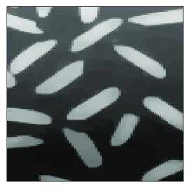
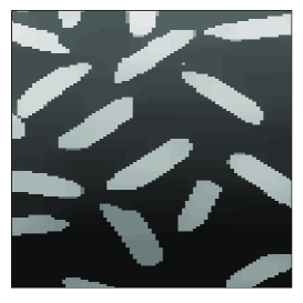
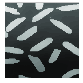
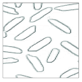
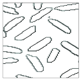
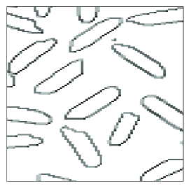
$(a)$	$(b)$	$(c)$

Figure 6: Detail of segmented images and their gradient $(a)$ for SC penalty using 3MG, $\lambda=2$, $\delta=0.2$, $(b)$ for NSNC penalty using TRW, $\lambda=1550$, $\delta=3.5$, and $(c)$ for SNC(iii) penalty using 3MG, $\lambda=1500$, $\delta=8$.

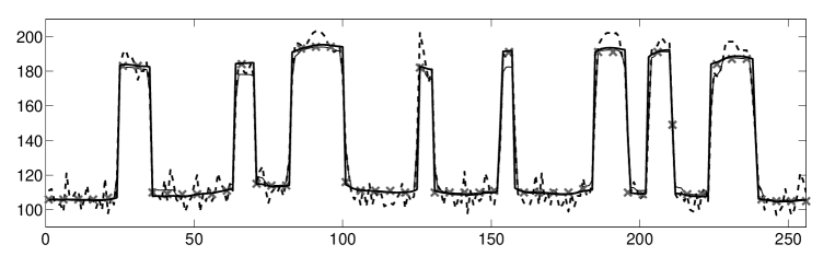
Figure 7: Comparison of $50$th line of segmented images using SC (thin line), NSNC (crosses) and SNC(iii) (thick line) potential functions. The $50$th line of the original image is indicated in dotted plot.

In the second experiment, we consider the segmentation of Rice image of size $N=256\times 256$ (see Figure 5). We define the segmented image as a minimizer of $F_{\delta}$, where ${\mathb{H}}={\mathb{I}}$, ${\mathb{y}}$ identifies with the original image and $(\forall{\mathb{z}}\in{\mathbb{R}}^{N})$ $\Phi({\mathb{z}})=\frac{1}{2}\|{\mathb{z}}\|^{2}$. The anisotropic penalization term is again used with $\tau=0$ for the same reason as earlier. Figs. 5 and 6 illustrate the resulting images and their gradient for SC, NSNC and SNC(iii) penalty functions, when regularization parameters $(\lambda,\delta)$ are tuned in order to obtain the best visual results in terms of segmentation. The gradients of the resulting images are evaluated by displaying, for every $n\in\left\{1,\dots,N\right\}$, $G_{n}=\|{\boldsymbol{\Delta}}_{n}\widehat{{\mathb{x}}}\|$ with ${\boldsymbol{\Delta}}_{n}=[{\boldsymbol{\Delta}}_{n}^{\mathrm{h}}\;\;{\boldsymbol{\Delta}}_{n}^{\mathrm{v}}]^{\top}\in{\mathbb{R}}^{2\times N}$ where ${\boldsymbol{\Delta}}_{n}^{\mathrm{h}}\in{\mathbb{R}}^{N}$ and ${\boldsymbol{\Delta}}_{n}^{\mathrm{v}}\in{\mathbb{R}}^{N}$ represent the first-order difference operators in the horizontal and vertical directions. Finally, the intensity values along the (arbitrarily chosen) $50$th line of each image are plotted in Figure 7 to better illustrate the behaviors of the different approaches.

Penalty function$(\lambda,\delta)$	Algorithm	Iteration	Time	$F_{\delta}$
SC $(2,0.2)$	3MG	$132$	$0.99$	$6.69\cdot 10^{6}$
	[NLCG-HS]	$144$	$1.49$	$6.69\cdot 10^{6}$
	[NLCG-PRP+]	[$143$]	[$1.47$]	[$6.69\cdot 10^{6}$]
	[NLCG-LS]	[$148$]	[$1.54$]	[$6.69\cdot 10^{6}$]
	L-BFGS	$215$	$3.44$	$6.69\cdot 10^{6}$
	HQ	$898$	$18.19$	$6.69\cdot 10^{6}$
SNC(iii) $(1500,8)$	3MG	[$491$]	[$3.43$]	$1.59\cdot 10^{7}$
	[NLCG-HS]	$1578$	$14.93$	$1.59\cdot 10^{7}$
	[NLCG-PRP+]	[$463$]	[$4.25$]	[$1.59\cdot 10^{7}$]
	[NLCG-LS]	[$598$]	[$5.64$]	[$1.59\cdot 10^{7}$]
	L-BFGS	$632$	$9.57$	$1.59\cdot 10^{7}$
	HQ	$3553$	$65.2$	$1.59\cdot 10^{7}$
NSNC $(1550,3.5)$	$\alpha$-EXP	$9$	$57.97$	$5.58\cdot 10^{6}$
	QCSM	$1$	$7.05$	$5.52\cdot 10^{6}$
	TRW	$5$	$6.71$	$5.52\cdot 10^{6}$
	BP	$50$	$61.83$	$5.52\cdot 10^{6}$

Table 5: Results for the segmentation problem.

According to Tab. 5, the best performance in terms of computational time is obtained by the 3MG algorithm with the SC penalty. However, the convex penalization strategy leads to poor segmentation results. Indeed, the boundaries of the reconstructed image are smooth and the background suffers from staircasing effect. In contrast, the nonconvex penalties give rise to truly piecewise constant images. The considered algorithms for the truncated quadratic penalty lead to segmented images very similar to the one obtained with SNC regularization. However, Tab. 5 shows that they are more demanding in terms of computational time than 3MG.

5.3 Image deblurring

Our third experiment corresponds to the problem of restoring the montage image $\overline{x}$, with size $256\times 256$, from blurred and noisy observations ${\mathb{u}}={\mathb{R}}\overline{{\mathb{x}}}+{\mathb{w}}$ where ${\mathb{w}}$ is a realization of a zero-mean white Gaussian noise and ${\mathb{R}}$ models a linear uniform blur with size $3\times 3$. The recovery of the original image is performed by solving (1) with $Q=2N$,

$${\mathb{H}}=\left[\begin{array}[]{c}{\mathb{R}}\\ {\mathb{I}}\end{array}\right]\qquad{\mathb{y}}=\left[\begin{array}[]{c}{\mathb{u}}\\ {\mathbf{0}}\end{array}\right],$$

and

$$(\forall{\mathb{z}}=(z_{q})_{1\leq q\leq 2N})\qquad\Phi({\mathb{z}})=\frac{1}{2}\left(\sum_{q=1}^{N}z_{q}^{2}+\beta\sum_{q=N+1}^{2N}d_{B}^{2}(z_{q})\right),$$

where $d_{B}$ denotes the distance to the closed convex interval $B=[0,255]$ and $\beta=0.01$. Furthermore, function $\Psi_{\delta}$ is given by (3) with $\tau=10^{-10}$ and $S=2N$. We consider, for every $s\in\{1,\ldots,N\}$, an isotropic regularization between neighbooring pixels, i.e., $P_{s}=2$ and ${\mathb{V}}_{s}=[{\boldsymbol{\Delta}}_{s}^{\mathrm{h}}\;\;{\boldsymbol{\Delta}}_{s}^{\mathrm{v}}]^{\top}$ where ${\boldsymbol{\Delta}}_{s}^{\mathrm{h}}\in{\mathbb{R}}^{N}$ (resp. ${\boldsymbol{\Delta}}_{s}^{\mathrm{v}}\in{\mathbb{R}}^{N}$) corresponds to a horizontal (resp. vertical) gradient operator, and, for every $s\in\{N+1,\ldots,2N\}$, the Hessian-based penalization from [38] i.e., $P_{s}=3$ and ${\mathb{V}}_{s}=[{\boldsymbol{\Delta}}_{s}^{\mathrm{hh}}\;\;\sqrt{2}{\boldsymbol{\Delta}}_{s}^{\mathrm{hv}}\;\;{\boldsymbol{\Delta}}_{s}^{\mathrm{vv}}]^{\top}$ where ${\boldsymbol{\Delta}}_{s}^{\mathrm{hh}}\in{\mathbb{R}}^{N}$, ${\boldsymbol{\Delta}}_{s}^{\mathrm{hv}}\in{\mathbb{R}}^{N}$ and ${\boldsymbol{\Delta}}_{s}^{\mathrm{vv}}\in{\mathbb{R}}^{N}$ model the second-order finite difference operators between neighbooring pixels, as described in [38, Sec.III-A]. For $s\in\{N+1,\ldots,2N\}$ we consider the $\ell_{2}-\ell_{1}$ function $\psi_{s,\delta}\colon t\mapsto\rho(\sqrt{1+{t^{2}/(\theta\delta)^{2}}}-1)$, where $\rho$ and $\theta$ take positive values. Tab. 6 presents the results for SC and SNC(ii) regularization of the image gradient (i.e. $\psi_{s,\delta}$ for $s\in\{1,\ldots,N\}$ ). Parameters $(\rho,\theta,\lambda,\delta)$ are tuned to maximize the SNR of the restored image. In both cases, the 3MG algorithm outperforms the three considered descent algorithms in terms of time efficiency. Additionally, the nonconvex strategy leads to better results in terms of SNR (see Figure 9). One can also observe that in this case the staircasing effect is reduced (see some image details in Figure 9).

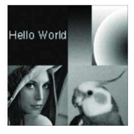
$(a)$	$(b)$

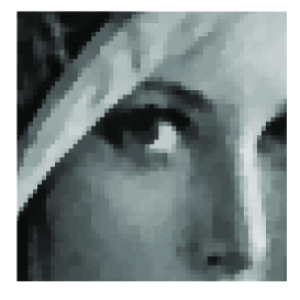
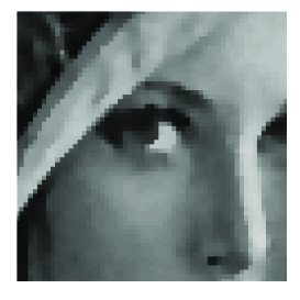
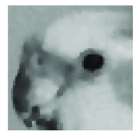
Figure 8: $(a)$ Original image with $256\times 256$ pixels and $(b)$ blurred noisy image with SNR$=18.65$ dB, MSSIM $=0.82$, $3\times 3$ uniform blur, noise standard deviation equal to $4$.

$(a)$	$(b)$

Figure 9: Deblurring results with $(a)$ SC penalty using 3MG, $\rho=0.56$, $\theta=0.18$, $\lambda=0.042$, $\delta=4.19$, SNR = $26.90$ dB, MSSIM = $0.94$ and $(b)$ with SNC(ii) penalty using 3MG, $\rho=41.55$, $\theta=0.86$, $\lambda=3.68$, $\delta=18.65$, SNR = $27.69$ dB, MSSIM = $0.94$.

Penalty function$(\rho,\theta,\lambda,\delta)$	Algorithm	Iteration	Time	$F_{\delta}$	SNR
SC $(0.56,0.18,0.042,4.19)$	3MG	$121$	$\underline{8.36}$	$8.22\cdot 10^{6}$	$26.90$
	NLCG-HS	$121$	$8.92$	$8.22\cdot 10^{6}$	$26.90$
	NLCG-PRP+	$129$	$9.32$	$8.22\cdot 10^{6}$	$26.90$
	NLCG-LS	$131$	$9.51$	$8.22\cdot 10^{6}$	$26.90$
	L-BFGS	$162$	$12.42$	$8.22\cdot 10^{6}$	$26.90$
	HQ	$418$	$94.3$	$8.22\cdot 10^{6}$	$26.90$
SNC(ii) $(41.55,0.86,3.68,18.65)$	3MG	$196$	$\underline{11.58}$	$7.92\cdot 10^{6}$	$27.69$
	NLCG-HS	$243$	$15.93$	$7.92\cdot 10^{6}$	$27.69$
	NLCG-PRP+	$221$	$14.41$	$7.92\cdot 10^{6}$	$27.69$
	NLCG-LS	$246$	$15.62$	$7.92\cdot 10^{6}$	$27.69$
	L-BFGS	$216$	$14.78$	$7.92\cdot 10^{6}$	$27.69$
	HQ	$616$	$104.9$	$7.92\cdot 10^{6}$	$27.69$

Table 6: Results for the deblurring problem.

5.4 Image reconstruction

In our last experiment, we consider the problem of reconstructing an image $\overline{{\mathb{x}}}\in{\mathbb{R}}^{N}$ from noisy tomographic acquisitions, modeled as

$${\mathb{u}}={\mathb{R}}\,{\mathb{x}}+{\mathb{w}},$$ (67)

where ${\mathb{R}}$ is the Radon projection matrix whose $(r,n)$ element ($1\leq r\leq R$, $1\leq n\leq N$) models the contribution of the $n$th pixel to the $r$th datapoint, and ${\mathb{w}}$ represents an additive noise component. In this example, we consider one slice of the standard Zubal phantom [64] with dimensions $N=128\times 128$, and $R=46336$ measurements from $181$ projection lines and $256$ angles. This image is corrupted with a zero-mean independent and identically distributed Laplacian noise (SNR = $23.5$ dB). Figure 12 shows the original image and its noisy sinogram.

The reconstruction is performed by minimizing $F_{\delta}$ with $Q=R+N$,

$${\mathb{H}}=\left[\begin{array}[]{c}{\mathb{R}}\\ {\mathb{I}}\end{array}\right]\qquad{\mathb{y}}=\left[\begin{array}[]{c}{\mathb{u}}\\ {\mathbf{0}}\end{array}\right],$$ (68)

and

$$(\forall{\mathb{z}}=(z_{q})_{1\leq q\leq Q})\qquad\Phi({\mathb{z}})=\frac{1}{2}\left(\sum_{q=1}^{R}\sqrt{1+(z_{q}/\rho)^{2}}+\beta\sum_{q=R+1}^{Q}d_{B}^{2}(z_{q})\right)$$ (69)

with $B=[0,255]$. Thus, $\Phi$ has a Lipschitz gradient with constant $L=\max(\frac{1}{2\rho^{2}},\beta)$. In the sequel, we take $\beta=10^{-2}$. Furthermore, the regularization function (3), with $\tau=10^{-10}$ and an isotropic edge-preserving penalty is considered i.e., $S=N$ and, for every $s\in\{1,\ldots,N\}$, $P_{s}=2$ and ${\mathb{V}}_{s}=[{\boldsymbol{\Delta}}_{s}^{\mathrm{h}}\;\;{\boldsymbol{\Delta}}_{s}^{\mathrm{v}}]^{\top}$ where ${\boldsymbol{\Delta}}_{s}^{\mathrm{h}}\in{\mathbb{R}}^{N}$ (resp. ${\boldsymbol{\Delta}}_{s}^{\mathrm{v}}\in{\mathbb{R}}^{N}$) corresponds to a horizontal (resp. vertical) gradient operator.

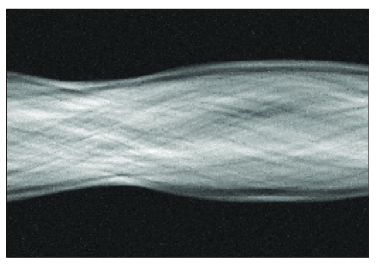
$(a)$	$(b)$

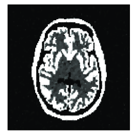
Figure 10: $(a)$ Initial gray level image with $128\times 128$ pixels and $(b)$ noisy sinogram with SNR=$23.5$ dB.

$(a)$	$(b)$

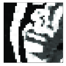
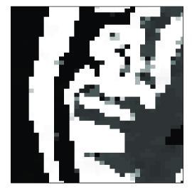
Figure 11: Reconstructed image using $(a)$ SC penalty function with 3MG, $\lambda=0.06$, $\delta=2.9$, $\rho=1.6$, SNR = $18.05$ dB, MSSIM = $0.81$, or $(b)$ using SNC(ii) penalty function with 3MG, $\lambda=1.2$, $\delta=11.1$, $\rho=2.2$, SNR = $21.13$ dB, MSSIM = $0.92$.

$(a)$	$(b)$	$(c)$

Figure 12: $(a)$ Detail of the original image and corresponding reconstructions with $(b)$ convex penalty function and $(c)$ nonconvex penalty function.

Figure 12 shows the results obtained for penalization strategies SC and SNC(ii), with $(\lambda,\delta,\rho)$ tuned to maximize the SNR of the restored image. We note that the SNC penalty leads to better results in terms of reconstruction quality. In particular, it appears to be well-suited to the reconstruction of the boundaries of the image, as demonstrated in Figure 12. Tab. 7 illustrates the performance of the 3MG algorithm, in comparison with the three tested descent algorithms, when either the SC or the SNC(ii) penalty function is used. In this example, the proposed algorithm outperforms the others, in terms of both iteration number and computational time. In the nonconvex case, because of the presence of local minimizers, the four algorithms do not lead to the same final SNR value. It can be noticed that the smallest final criterion value is obtained with the 3MG algorithm.

Penalty function$(\lambda,\delta,\rho)$	Algorithm	Iteration	Time	$F_{\delta}$	SNR
SC $(0.06,2.9,1.6)$	3MG	$253$	$59.3$	$1.1\cdot 10^{6}$	$18.05$
	[NLCG-HS]	$358$	$84.1$	$1.1\cdot 10^{6}$	$18.05$
	[NLCG-PRP+]	[$410$]	[$96.4$]	[$1.1\cdot 10^{6}$]	[$18.05$]
	[NLCG-LS]	[$507$]	[$141.3$]	[$1.1\cdot 10^{6}$]	[$18.05$]
	L-BFGS	$349$	$82.3$	$1.1\cdot 10^{6}$	$18.05$
	HQ	$728$	$337$	$1.1\cdot 10^{6}$	$18.05$
SNC(ii) $(1.2,11.1,2.2)$	3MG	$516$	$119.8$	$8.6214\cdot 10^{6}$	$21.13$
	[NLCG-HS]	$618$	$143$	$8.6228\cdot 10^{6}$	$20.89$
	[NLCG-PRP+]	[$876$]	[$204$]	$8.6229\cdot 10^{6}$	$20.89$
	[NLCG-LS]	[$1212$]	[$360$]	[$8.6228\cdot 10^{6}$]	[$20.89$]
	L-BFGS	$870$	$203$	$8.6225\cdot 10^{6}$	$21.17$
	HQ	$1152$	$530$	$8.6236\cdot 10^{6}$	$20.85$

Table 7: Results for the tomography problem.

6 Conclusion

In this work, we have considered a class of smooth nonconvex regularization functions and we have proposed an efficient minimization strategy for solving the associated variational problems in imaging applications. Connections with $\ell_{0}$ penalized problems were given asymptotically. In addition, a novel convergence proof of the proposed subspace MM algorithm relying on the Kurdyka-Łojasiewicz inequality was given. Numerical experiments were carried out to compare the proposed approach with other state-of-the art continuous optimization methods (both for nonconvex and convex penalizations) and with discrete optimization approaches dealing with a truncated quadratic penalization. In the four presented image processing examples, we argue that the proposed approach constitutes an appealing alternative to the existing methods in terms of recovered image quality and computational time.

References

- [1] M. Allain, J. Idier, and Y. Goussard, On global and local convergence of half-quadratic algorithms, IEEE Trans. Image Process., 15 (2006), pp. 1130–1142.
- [2] A. Antoniadis, D. Leporini, and J.-C. Pesquet, Wavelet thresholding for some classes of non-Gaussian noise, Statist. Neerlandica, 56 (2002), pp. 434–453.
- [3] H. Attouch and J. Bolte, On the convergence of the proximal algorithm for nonsmooth functions involving analytic features, Math. Prog., 116 (2008), pp. 5–16.
- [4] H. Attouch, J. Bolte, P. Redont, and A. Soubeyran, Proximal alternating minimization and projection methods for nonconvex problems. An approach based on the Kurdyka-Łojasiewicz inequality, Math. Oper. Res., 35 (2010), pp. 438–457.
- [5] H. Attouch, J. Bolte, and B. F. Svaiter, Convergence of descent methods for semi-algebraic and tame problems: proximal algorithms, forward backward splitting, and regularized Gauss-Seidel methods, Math. Prog., (2011), pp. 1–39.
- [6] H. H. Bauschke and P. L. Combettes, Convex Analysis and Monotone Operator Theory in Hilbert Spaces, Springer, New York, NY, 1st ed., 2011.
- [7] A. Ben-Tal and M. Teboulle, A smoothing technique for nondifferentiable optimization problems, in Optimization, vol. 1405 of Lecture Notes in Mathematics, Springer Berlin, 1989, pp. 1–11.
- [8] D. P. Bertsekas, Nonlinear Programming, Athena Scientific, Belmont, MA, 2nd ed., 1999.
- [9] M. Black, G. Sapiro, D. Marimont, and D. Heeger, Robust anisotropic diffusion, IEEE Transactions on Image Processing, 7 (1998), pp. 421 –432.
- [10] J. Bolte, P. L. Combettes, and J.-C. Pesquet, Alternating proximal algorithm for blind image recovery, in Proc. IEEE International Conference on Image Processing (ICIP), Hong Kong, September 2010, pp. 1673 –1676.
- [11] J. Bolte, A. Daniilidis, and A. Lewis, The Łojasiewicz inequality for nonsmooth subanalytic functions with applications to subgradient dynamical systems, SIAM J. Optim., 17 (2006), pp. 1205–1223.
- [12] J. Bolte, A. Daniilidis, A. Lewis, and M. Shiota, Clarke subgradients of stratifiable functions, SIAM J. Optim., 18 (2007), pp. 556–572.
- [13] Y. Boykov, O. Veksler, and R. Zabih, Fast approximate energy minimization via graph cuts, IEEE Trans. Pattern Anal. Mach. Intell., 23 (2001), pp. 1222 –1239.
- [14] E. J. Candes, The restricted isometry property and its implications for compressed sensing, C. R. Math., 346 (2008), pp. 589–592.
- [15] J. Cantrell, Relation between the memory gradient method and the Fletcher-Reeves method, J. Optim. Theory Appl., 4 (1969), pp. 67–71.
- [16] P. Charbonnier, L. Blanc-Féraud, G. Aubert, and M. Barlaud, Deterministic edge-preserving regularization in computed imaging, IEEE Trans. Image Process., 6 (1997), pp. 298–311.
- [17] E. Chouzenoux, J. Idier, and S. Moussaoui, A Majorize-Minimize strategy for subspace optimization applied to image restoration, IEEE Trans. Image Process., (2011), pp. 1517–1528.
- [18] E. Chouzenoux, J.-C. Pesquet, H. Talbot, and A. Jezierska, A memory gradient algorithm for - regularization with applications to image restoration, in Proc. IEEE International Conference on Image Processing (ICIP), Brussels, Belgium, September 2011.
- [19] M. Davenport, M. F. Duarte, Y. C. Eldar, and G. Kutyniok, Introduction to compressed sensing, Cambridge University Press, 2012.
- [20] A. H. Delaney and Y. Bresler, Globally convergent edge-preserving regularized reconstruction: an application to limited-angle tomography, IEEE Trans. Image Process., 7 (1998), pp. 204 –221.
- [21] J. E. Dennis and R. E. Welsch, Techniques for nonlinear least squares and robust regression, Communications in Statistics - Simulation and Computation, 7 (1978), pp. 345–359.
- [22] D. L. Donoho, Neighborly polytopes and sparse solutions of underdetermined linear equations, tech. report, University of Stanford, 2005.
- [23] M. Elad, B. Matalon, and M. Zibulevsky, Coordinate and subspace optimization methods for linear least squares with non-quadratic regularization, Appl. Comput. Harmon. Anal., 23 (2006), pp. 346–367.
- [24] M. Elad, P. Milanfar, and R. Rubinstein, Analysis versus synthesis in signal priors, Inverse Prob., 23 (2007), pp. 947–968.
- [25] Y. C. Eldar, P. Kuppinger, and H. Bolcskei, Block-sparse signals: uncertainty relations and efficient recovery, IEEE Trans. Signal Process., 58 (2010), pp. 3042 –3054.
- [26] P. Felzenszwalb and D. Huttenlocher, Efficient belief propagation for early vision, Int. J. Computer Vision, 70 (2006), pp. 41–54.
- [27] M. Fornasier and F. Solombrino, Linearly constrained nonsmooth and nonconvex minimization, tech. report, January 2012. http://arxiv.org/abs/1201.6069.
- [28] S. Geman and D. E. McClure, Bayesian image analysis: An application to single photon emission tomography, in In Proc. Statist. Comput. Sect., American Statistical Association, 1985, pp. 12–18.
- [29] W. W. Hager and H. Zhang, A survey of nonlinear conjugate gradient methods, Pacific J. Optim., 2 (2006), pp. 35–58.
- [30] T. J. Hebert and R. Leahy, Statistic-based MAP image reconstruction from poisson data using Gibbs priors, IEEE Trans. Signal Process., 40 (1992), pp. 2290–2303.
- [31] P. J. Huber, Robust Statistics, John Wiley, New York, NY, 1981.
- [32] M. Hyder and K. Mahata, An approximate norm minimization algorithm for compressed sensing, in Proc. IEEE International Conference on Acoustics, Speech and Signal Processing (ICASSP), Taipei, Taiwan, April 2009, pp. 3365 –3368.
- [33] A. Jezierska, H. Talbot, O. Veksler, and D. Wesierski, A fast solver for truncated-convex priors: quantized-convex split moves, in Energy Minimization Methods in Computer Vision and Pattern Recognition, Y. Boykov, F. Kahl, V. Lempitsky, and F. Schmidt, eds., vol. 6819 of Lecture Notes in Computer Science, Springer Berlin / Heidelberg, 2011, pp. 45–58.
- [34] V. Kolmogorov, Convergent tree-reweighted message passing for energy minimization, IEEE Trans. Pattern Anal. Mach. Intell., 28 (2006), pp. 1568 –1583.
- [35] K. Kurdika and A. Parusinski, -stratification of subanalytic functions and the Łojasiewicz inequality, C.R. Acad. Sci., Ser. I: Math., 318 (1994), pp. 129–133.
- [36] C. Labat and J. Idier, Convergence of conjugate gradient methods with a closed-form stepsize formula, J. Optim. Theory Appl., 136 (2008), pp. 43–60.
- [37] K. Lange, Convergence of EM image reconstruction algorithms with Gibbs smoothing, IEEE Trans. Med. Imaging, 9 (1990), pp. 439–446.
- [38] S. Lefkimmiatis, A. Bourquard, and M. Unser, Hessian-based norm regularization for image restoration with biomedical applications, IEEE Trans. Image Process., 21 (2012), pp. 983–995.
- [39] D. C. Liu and J. Nocedal, On the limited memory BFGS method for large scale optimization, Math. Prog., 45 (1989), pp. 503–528.
- [40] S. Łojasiewicz, Une propriété topologique des sous-ensembles analytiques réels, Editions du centre National de la Recherche Scientifique, 1963, pp. 87–89.
- [41] M. Malek-Mohammadi, M. Babaie-Zadeh, and C. Jutten, SRF: matrix completion based on smoothed rank function, in Proc. IEEE International Conference on Acoustics, Speech, and Signal Processing (ICASSP), Praque, Czech Republic, May 2011, pp. 3672–3675.
- [42] P. Meer, D. Mintz, A. Rosenfeld, and D. Y. Kim, Robust regression methods for computer vision: a review, Int. J. Computer Vision, 6 (1991), pp. 59–70.
- [43] A. Miele and J. W. Cantrell, Study on a memory gradient method for the minimization of functions, J. Optim. Theory Appl., 3 (1969), pp. 459–470.
- [44] H. Mohimani, M. Babaie-Zadeh, and C. Jutten, A fast approach for overcomplete sparse decomposition based on smoothed norm, IEEE Trans. Signal Process., 57 (2009), pp. 289 –301.
- [45] M. Nikolova, Analysis of the recovery of edges in images and signals by minimizing nonconvex regularized least-squares, Multiscale Model. Simul., 4 (2005), pp. 960–991.
- [46] , Description of the minimizers of least squares regularized with norm. Uniqueness of the global minimizer, SIAM J. Imag. Sci., 6 (2013), pp. 904–937.
- [47] M. Nikolova, M. K. Ng, S. Zhang, and W.-K. Ching, Efficient reconstruction of piecewise constant images using nonsmooth nonconvex minimization, SIAM J. Imag. Sci., 1 (2008), pp. 2–25.
- [48] J. M. Ortega and W. C. Rheinboldt, Iterative solution of nonlinear equations in several variables, Academic Press, New York, 1970.
- [49] D. J. Peter, V. K. Govindan, and A. T. Mathew, Nonlocal-means image denoising technique using robust m-estimator, J. Comput. Sci. Techn., 25 (2010), pp. 623–631.
- [50] A. Raj, G. Singh, R. Zabih, B. Kressler, Y. Wang, N. Schuff, and M. Weiner, Bayesian parallel imaging with edge-preserving priors, Magn. Reson. Med., 57 (2007), pp. 8–21.
- [51] A. Raj and R. Zabih, A graph cut algorithm for generalized image deconvolution, in Proc. IEEE International Conference on Computer Vision (ICCV), Beijing, China, 2005, pp. 1048–1054.
- [52] M. Rivera and J. Marroquin, Efficient half-quadratic regularization with granularity control, 21 (2003), pp. 345–357.
- [53] R. T. Rockafellar and R. J.-B. Wets, Variational analysis, Springer-Verlag, 1st ed., 1997.
- [54] L. I. Rudin, S. Osher, and E. Fatemi, Nonlinear total variation based noise removal algorithms, Phys. D, 60 (1992), pp. 259–268.
- [55] A. Tikhonov and V. Arsenin, Solutions of Ill-Posed Problems, Winston, Washington, DC, 1977.
- [56] D. M. Titterington, General structure of regularization procedures in image restoration, Astron. Astrophys., 144 (1985), pp. 381–387.
- [57] O. Veksler, Efficient graph-based energy minimization methods in computer vision, PhD thesis, Cornell University, Ithaca, NY, USA, 1999.
- [58] , Graph cut based optimization for MRFs with truncated convex priors, in Proc. IEEE International Conference on Computer Vision and Pattern Recongnition (ICCVPR), Minneapolis, MN, June 2007, pp. 1–8.
- [59] C. R. Vogel and M. E. Oman, Iterative methods for total variation denoising, SIAM J. Sci. Comput., 17 (1996), pp. 227–238.
- [60] Z. Wang, A. C. Bovik, H. R. Sheikh, and E. P. Simoncelli, Image quality assessment: from error visibility to structural similarity, IEEE Trans. Image Process., 13 (2004), pp. 600 –612.
- [61] Y. Zhang and N. Kingsbury, Restoration of images and 3D data to higher resolution by deconvolution with sparsity regularization, in Proc. IEEE International Conference on Image Processing (ICIP), Hong Kong, September 2010, pp. 1685 –1688.
- [62] M. Zibulevsky and M. Elad, - optimization in signal and image processing, IEEE Signal Process. Mag., 27 (2010), pp. 76–88.
- [63] H. Zou and T. Hastie, Regularization and variable selection via the elastic net, J. R. Statist. Soc. B, 67 (2005), pp. 301–320.
- [64] I. G. Zubal, C. R. Harrell, E. O. Smith, Z. Rattner, G. Gindi, and P. B. Hoffer, Computerized three-dimensional segmented human anatomy, Med. Phys., 21 (1994), pp. 299–302.