Topology of RNA-RNA interaction structures
Aarhus University, DK-8000 Århus C, Denmark
University of Southern Denmark, Campusvej 55, DK-5230 Odense M, Denmark
Center for Quantum Geometry of Moduli Spaces Aarhus University, DK-8000 Århus C, Denmark
Math and Physics Departments, California Institute of Technology, Pasadena, California, USA
Correspondent author: phone: +45 24409251
duck@santafe.edu
Abstract
The topological filtration of interacting RNA complexes is studied and the role is analyzed of certain diagrams called irreducible shadows, which form suitable building blocks for more general structures. We prove that for two interacting RNAs, called interaction structures, there exist for fixed genus only finitely many irreducible shadows. This implies that for fixed genus there are only finitely many classes of interaction structures. In particular the simplest case of genus zero already provides the formalism for certain types of structures that occur in nature and are not covered by other filtrations. This case of genus zero interaction structures is already of practical interest, is studied here in detail and found to be expressed by a multiple context-free grammar extending the usual one for RNA secondary structures. We show that in time and space complexity, this grammar for genus zero interaction structures provides not only minimum free energy solutions but also the complete partition function and base pairing probabilities.
Keywords: RNA interaction structure, topological genus, irreducible shadow, partition function
1. Introduction
RNA-RNA interactions constitute one of the fundamental mechanisms of cellular regulation. For instance, small RNAs binding a larger (m)RNA target include: the regulation of translation in both prokaryotes Narberhaus and Vogel (2007) and eukaryotes McManus and Sharp (2002); Banerjee and Slack (2002), the targeting of chemical modifications Bachellerie et al. (2002), insertion editing Benne (1992) and transcriptional control Kugel and Goodrich (2007). For a variety of RNA classes including miRNAs, siRNAs, snRNAs, gRNAs, and snoRNAs, a salient feature is the formation of RNA-RNA interaction structures that are far more complex than simple sense-antisense interactions. Accordingly, the ability to predict the details of RNA-RNA interactions in terms of the thermodynamics of binding and in its structural consequences is a necessary prerequisite to understanding RNA-based regulation mechanisms. The exact location of the binding and the subsequent impact of the interaction on the structure of the target molecule has potentially profound biological consequences. In case of sRNA-mRNA interactions, such details determine whether the sRNA is a positive or negative regulator of transcription depending on whether binding exposes or covers the Shine-Dalgarno sequence Sharma et al. (2007); Majdalani et al. (2002). Effects along these lines have been observed also using artificially designed opener and closer RNAs that regulate the binding of the HuR protein to human mRNAs Meisner et al. (2004); Hackermüller et al. (2005).
An RNA molecule is a linearly oriented sequence of four types of nucleotides, namely, A, U, C, and G. This sequence is endowed with a well-defined orientation from the - to the -end and referred to as the backbone. Each nucleotide can form a base pair by interacting with at most one other nucleotide by establishing hydrogen bonds. Here we restrict ourselves to Watson-Crick base pairs GC and AU as well as the wobble base pairs GU. In the following, base triples as well as other types of more complex interactions are neglected. RNA structures can be presented as diagrams by drawing the backbone horizontally and all base pairs as arcs in the upper halfplane; see Figure 1. This set of arcs provides our coarse-grained RNA structure in particular ignoring any spatial embedding or geometry of the molecule beyond its base pairs.

Accordingly, particular classes of base pairs translate into specific structure categories, the most prominent of which are secondary structures Kleitman (1970); Nussinov et al. (1978); Waterman and Smith (1978); Waterman (1979). When represented as diagrams, secondary structures have only non-crossing base pairs (arcs). Beyond RNA secondary structures are the RNA pseudoknot structures that allow for cross serial interactions Rivas and Eddy (1999). There are several meaningful filtrations of cross-serial interactions Orland and Zee (2002); Reidys et al. (2011, 2010). Given an RNA coarse-grained structure class together with an energy function, “folding” an RNA sequence means to compute a minimum111with respect to the a priori specified energy function free energy configuration (MFE) or a partition function for the sequence.
RNA interaction structures are structures over two backbones. We distinguish internal arcs and external arcs as having their endpoints on the same and different backbones, respectively. Interaction structures are represented as two backbones with internal and external arcs drawn in the upper halfplane. Alternatively, they can be represented by drawing the two backbones on top of each other, see Figure 2.

The simplest approach for folding RNA-RNA interaction structures concatenates two (or more) interacting sequences one after another remembering the specific merge point (cut-point) and then employs the standard secondary structure folding algorithm on a single strand with a slightly modified energy model that treats loops containing cut-points as external elements. The software tools RNAcofold Hofacker et al. (1994); Bernhart et al. (2006), pairfold Andronescu et al. (2005) and NUPACK Dirks et al. (2007) subscribe to this strategy. This approach falls short predicting many important motifs such as kissing-hairpin loops. The paradigm of concatenation has also been generalized to include cross-serial interactions Rivas and Eddy (1999). The resulting model, however, still does not generate all relevant interaction structures Chitsaz et al. (2009b); Qin and Reidys (2007). An alternative line of thought, implemented in RNAduplex and RNAhybrid Rehmsmeier et al. (2004), is to neglect all internal base pairings in either strand, i.e., to compute the minimum free energy (MFE) secondary structure of hybridization of otherwise unstructured RNAs. RNAup Mückstein et al. (2006, 2008) and intaRNA Busch et al. (2008) restrict interactions to a single interval that remains unpaired in the secondary structure for each partner. As a special case, snoRNA/target complexes are treated more efficiently using a specialized tool Tafer et al. (2009) due to the highly conserved interaction motif. Algorithmically, the approaches mentioned so far are close relatives of the “classical” RNA folding recursions given by Zuker and Sankoff (1984); Waterman and Smith (1978). A different approach was taken independently by Pervouchine (2004) and Alkan et al. (2006), who proposed MFE folding algorithms for predicting the AP-structure of two interacting RNA molecules. In this model, the intramolecular structures of each partner are pseudoknot-free, the intermolecular binding pairs are non-crossing, and there is no so-called “zig-zag” motif, see Sec. 2. The optimal joint structure can be computed in time and space by means of dynamic programming.
In contrast to the RNA secondary folding problem, where minimum energy folding and partition functions can be obtained by similar algorithms, the case of interaction structures is more involved. The reason is that simple unambiguous grammars are known for RNA secondary structures Dowell and Eddy (2004) while the disambiguation of grammar underlying the Alkan-Pervouchine algorithm requires the introduction of a large number of additional non-terminals (which algorithmically translate into additional dynamic programming tables). The partition function was derived independently by Chitsaz et al. (2009b) (piRNA) and Huang et al. (2009) (rip1). In Huang et al. (2010), probabilities of interaction regions as well as entire hybrid blocks were derived. Although the partition function of joint structures can also be computed in time and space, the current implementations require large computational resources. Salari et al. (2009) recently achieved a substantial speed-up making use of the observation that the external interactions mostly occur between pairs of unpaired regions of single structures. Chitsaz et al. (2009a), on the other hand, use tree-structured Markov Random Fields to approximate the joint probability distribution of multiple contact regions. The RNA-RNA interaction structures of Huang et al. (2010); Alkan et al. (2006); Hofacker et al. (1994); Bernhart et al. (2006) have the following features:
-
•
when drawing the two backbones on top of each other, all base pairs are non-crossing, i.e., no pseudoknots formed by internal or external arcs are allowed,
-
•
zig-zag motifs are disallowed.
This paper will relax the above constraints and propose a novel filtration of RNA-RNA interaction structures based on the topological fitration of RNA interaction structures. Interaction structures that do not belong to the Alkan-Pervouchine class exist: for instance the integral RNA (hTER) of the human telomerase ribonucleoprotein has a conserved secondary structure that contains a potential pseudoknot Ly et al. (2003). There is evidence that the two conserved complementary sequences of one stem of the hTER pseudoknot domain can pair intermolecularly in vitro, and that formation of this stem as part of a novel “transpseudoknot” is required for the telomerase to be active in its dimeric form. The classification and expansion of pseudoknotted RNA structures over one backbone via topological genus of the associated fatgraph were first proposed by Orland and Zee (2002); Penner (2004); Bon et al. (2008)
In Reidys et al. (2011); Zagier (1995), it was proved that for any genus, there are only finitely many shadows, i.e., particular, simple atomic motifs. In case of genus one, these shadows were first presented in Bon et al. (2008). Shadows give rise to a novel structure class, naturally generalizing RNA secondary structures. These -structures Reidys et al. (2011) are generated by concatenation and nesting of irreducible building blocks of genus . We shall present the topological classification of RNA-RNA interaction structures. This filtration gives rise to the notion of -structures over two backbones. In analogy to their one-backbone counterparts, -structures over two backbones are composed of irreducible building blocks of genus and have accordingly arbitrarily high genus. We shall see that for any fixed genus, there are only finitely many irreducible shadows over two backbones. In particular, we study genus zero structures over two backbones. The latter are the two backbone analogue of RNA secondary structures222which are well-known to be genus zero structures over one backbone. -structures over two backbones already exhibit interesting features not shared with AP-structures, see Figure 3.
We furthermore derive an unambiguous grammar for -structures over two backbones, which translates into an efficient dynamic programming algorithm. This grammar, illustrated in Figure 4, allows the calculation of the minimum free energy, partition function and Boltzmann-sampling. It explicitly treats hybrids and gap structures, i.e., maximal regions with exclusively intermolecular interactions and maximal regions with base pairs over one backbone. The grammar thus facilitates the computation of the probability of hybrids, the target interaction probability between two RNA strands, and the probability of gap structures.
2. Basic facts
2.1. Diagrams
A diagram is a labeled graph over the vertex set in which each vertex has degree , represented by drawing its vertices in a horizontal line and its arcs , where , in the upper half-plane. A backbone is a sequence of consecutive integers contained in . A diagram over backbones is a diagram together with a partition of into backbones, see Figure 1 (B). In the following we shall denote the set of diagrams over one and two backbones by and respectively.
The vertices and arcs of a diagram correspond to nucleotides and base pairs, respectively. For a diagram over backbones, the leftmost vertex of each backbone denotes the end of the RNA sequence, while the rightmost vertex denotes the end. In case of , we shall distinguish two types of arcs: an arc is called exterior if it connects different backbones and interior otherwise. Diagrams over backbones without exterior arcs are disjoint unions of diagrams over one backbone.
The particular case is referred to as RNA interaction structures Huang et al. (2009, 2010), see Figure 2 (A). As mentioned before, interaction structures are oftentimes represented alternatively by drawing the two backbones and on top of each other, indexing the vertices to be the end of and to be the of .
A zig-zag is defined as follows: given two sequences and , suppose that , (i.e., is base paired with ), , and with and . We say that is subsumed in , if for any , implies . Finally, a zigzag is a subgraph containing two dependent interior arcs and neither one subsuming the other, see Figure 5, where dependence here means that there exists at least one exterior arc such that and .

2.2. From diagrams to topological surfaces
One approach for deriving meaningful filtrations of RNA structure is to pass from diagrams to topological surfaces Massey (1967). It is natural to make this transition from combinatorics to topology via fatgraphs Penner et al. (2010); Penner (2011). A fatgraph , sometimes also called “ribbon graph” or “map”, is a graph together with a collection of cyclic orderings, called a fattening, one such ordering on the half-edges incident on each vertex. Each fatgraph determines an oriented surface as follows: let be the set of -vertices and be the set of -edges. For each , consider an oriented surface isomorphic to a polygon with sides containing in its interior where is the valence of . The incident edges of are also incident to a univalent vertex contained in alternating sides of , which are identified with the incident half-edges in the natural way so that the induced counter-clockwise cyclic ordering on the boundary of agrees with the fattening of about . The surface is the quotient of the disjoint union , where the frontier edges, which are oriented with the polygons on their left, are identified by an orientation-reversing homeomorphism if the corresponding half-edges lie in a common edge of . This defines the oriented surface , which is connected if and only if is and is uniquely determined in this case by its genus and number of boundary components. Since contains as a deformation retract, they share the Euler characteristic , and the genus of is given by .
For an RNA diagram, we may draw a representation as usual so that the backbone is a horizontal line oriented from left to right, and the arcs lie in the upper half-plane. This determines a unique fattening on any diagram, cf. the leftmost two panels in Figure 6 for the fatgraph and its corresponding surface. Each boundary component of determines a closed edge-path or cycle on , oriented with the surface lying on its left. In particular, a neighborhood of each edge inherits an orientation from that of which combine to give the oriented cycles as depicted in the third panel of Figure 6. Without affecting topological type of the constructed surface, one may collapse each backbone to a single vertex with the induced fattening called the polygonal model of the RNA, as illustrated in the rightmost panels in Figure 6. It is the orientation of each backbone from the ’end to the end that allows us to transform the fatgraph of an RNA-structure or RNA-interaction into a fatgraph with one or two vertices.
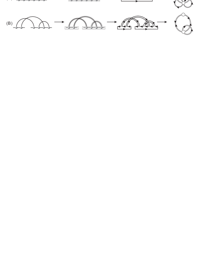
This backbone-collapse preserves orientation, Euler characteristic and genus by construction. It is reversible by inflating each vertex to form a backbone. Using the collapsed fatgraph representation, we see that for a connected diagram over backbones, the genus of the surface (with boundary) is determined by the number of arcs as well as the number of boundary components, namely, , cf. Figure 6.
Diagrams over one and two backbones are related by gluing, i.e., we have the mapping
where is obtained by keeping all arcs in and connecting the end of and the end of , see Figure 7 (A).
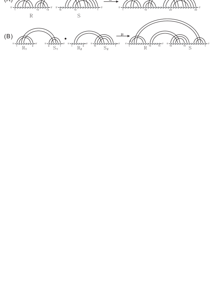
In addition to gluing, there is another operation mapping a pairs of diagram over two backbones into a diagram over two backbones: given two diagrams over two backbones, we can insert into the gap of by concatenating the backbones and and and preserving orientation.; see Figure 7 (B). This composition is by construction again a diagram over two backbones denoted , i.e., we have a mapping
| (2.1) |
It is straightforward to see that is an associative product with unit given by the diagram over two empty backbones. The product is not commutative.
3. Shadows
Definition 1.
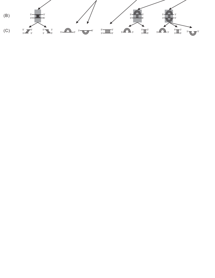
A stack in a diagram is a maximal collection of parallel arcs of the form . An arc is non-crossing if there is no other arc in the diagram that crosses it, and a vertex is isolated if it has no arcs incident upon it. A shadow is a diagram with no non-crossing arcs or isolated vertices so that each stack has size one, and a shadow is non-trivial provided each backbone contains at least one paired vertex.
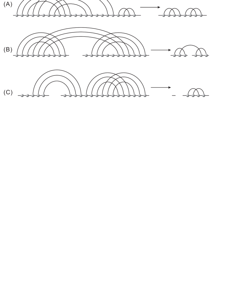
A diagram determines a shadow by removing all non-crossing arcs, deleting all isolated vertices and collapsing each induced stack to a single arc as in Figure 8. We shall denote the shadow of a diagram by , so . Projecting into the shadow does not affect genus, i.e., . In case there are no crossing arcs, becomes an empty diagram on the same number of backbones as as in Figure 8 (C). By definition, any empty backbone contributes one boundary component. For example, for a diagram over backbones that contains no crossing arcs, is a sequence of empty backbones with boundary components.
Let us begin by refining an observation about shadows over one backbone from Reidys et al. (2011):
Theorem 1.
Shadows of genus over one backbone have the following properties:
(a)
a shadow of genus contains at least and at most arcs; in particular
for fixed genus, there are only finitely many shadows;
(b) for any , there exists a shadow of genus containing
exactly arcs.
Proof.
First note that if there is more than one boundary component, then there must be an arc with different boundary components on its two sides and removing this arc decreases by exactly one while preserving since the number of arcs is given by . Furthermore, if there are boundary components of length in the polygonal model, then since each side of each arc is traversed once by the boundary. For a shadow, by definition, and as one sees directly. It therefore follows that , so , i.e., . Thus, we have , i.e., any shadow can contain at most arcs. The lower bound follows directly from since .
Let be a shadow containing mutually crossing arcs, i.e., each arc crosses any of the remaining arcs. has genus and contains a unique boundary component of length , i.e., traversing non-backbone arcs counted with multiplicity. We construct a new shadow of genus containing arcs, by inserting an arc crossing into from the end of such that the boundary component in splits into one boundary component of length and another of length . The latter becomes the first boundary component of . The newly inserted arc is by construction crossing, splits a boundary component and preserves genus. We now prove the assertion by induction of the number of inserted arcs. By the induction hypothesis, there exists a shadow of genus having arcs, whose first boundary component has length . Again, we insert a crossing arc as described above thereby splitting the first boundary component into one of length and the other of length . After such insertions, we arrive at a shadow whose first boundary component has length while all other boundary components have length . Accordingly, there exists a set of shadows all having genus , where each contains arcs, see Figure 9. ∎

Corollary 1.
A shadow over two backbones has the following properties:
(a)
a shadow of genus over two backbones contains at least
and at most arcs; a shadow of genus has at least and
at most arcs.
in particular, the set of such shadows is finite;
(b)
for any in case of and
in case of , there exists some shadow over two
backbones with genus containing exactly arcs.
Proof.
We first claim that any shadow of genus over two backbones can be obtained by cutting the backbone of a shadow over one backbone having either genus or . To see this, suppose we are given a shadow of genus , having boundary components and arcs so that , i.e., , where . Cutting the backbone then either splits a boundary component, or merges two distinct boundary components. Since cutting does not affect arcs and increases the number of backbones by one we have the resulting genus
as was claimed. We next observe that a shadow of genus over two backbones has at least arcs, while the maximum number of arcs contained in such a shadow is given by . For , it is impossible to cut a shadow of genus having arcs and keep the genus. Thus the shadow of genus over two backbones has at least arcs. We can always map an arbitrary shadow over two backbones of genus via into a shadow over one backbone, whence the assertion. Theorem 1 guarantees that there are only finitely many such shadows, and the corollary follows. ∎
Corollary 2.
There exist exactly seven non-trivial shadows over two backbones having genus .
Proof.
There exists no non-trivial shadow over one backbone of genus since -structures over one backbone are secondary structures containing exclusively non-crossing arcs. In view of Corollary 1, all non-trivial shadows over two backbones having genus are therefore obtained by cutting the backbone of shadows of genus over one backbone. By inspection, there are seven possible such cuts as in Figure 10. ∎

4. Irreducibility
Definition 2.
A diagram over backbones is called irreducible if and only if it is connected and for any two arcs, contained in , there exists a sequence of arcs such that are crossing.
We proceed by refining Theorem 1:
Corollary 3.
An irreducible shadow having genus over two backbones contains at least
and at most arcs, and for and ,
there exists an irreducible shadow of genus
over two backbones having exactly arcs.
An irreducible shadow having genus has the following properties:
(a)
every irreducible shadow with genus over two backbones contains at least
and at most arcs;
(b)
for arbitrary genus and any , there exists an
irreducible shadow of genus over one backbone having exactly
arcs.
Proof.
Definition 3.
Let be a diagram. We call an irreducible shadow of (irreducible -shadow) if and only if is an irreducible shadow and any arc in is contained in . Let .
Clearly, our notion of irreducibility recovers for diagrams over one
backbone that of Reidys et al. (2011); Bon et al. (2008).
A diagram over one backbone can iteratively be
decomposed by first removing all non-crossing arcs as well as isolated vertices
and second by removing irreducible -shadows iteratively as follows:
one removes (i.e., cuts the backbone at two points and after removal
merges the cut-points) irreducible -shadows from bottom to top,
i.e., such that there exists no irreducible -shadow that is nested
within the one previously removed.
if the removal of an irreducible -shadow induces the formation
of a non-trivial stack as in Figure 11, then it is collapsed into a
single arc.

We next extend the decomposition of diagrams over one backbone Reidys et al. (2011)
to diagrams over two backbones. Let be a diagram over two backbones.
By definition, irreducible -shadows over two backbones are either
connected or a disjoint union of two irreducible shadows over one backbone.
Thus, can be decomposed by removing first all non-crossing arcs as
well as any isolated vertices and second all irreducible -shadows in
two rounds as follows:
remove any irreducible -shadows over one backbone, from bottom
to top, as previously described, see Figure 12,
remove the irreducible -shadows over two backbones iteratively,
starting with the irreducible -shadow containing the leftmost
vertex of the second backbone, see Figure 12.

5. -structures over two backbones
Definition 4.
A diagram over backbones is a -structure over backbones if and only if we have for any irreducible -shadow .
With foresight, we refine the notion of irreducible -shadow as follows:
Lemma 1.
Suppose is a -structure over two backbones. Then
| (5.1) |
Proof.
By construction, is a shadow over one backbone consisting of irreducible components of genus at most . Thus, is a -structure and
| (5.2) |
Let be the set of -subshadows over two backbones where the backbones are on the same boundary component and let be those that are not. We have
| (5.3) |
Claim . Suppose , then
| (5.4) |
To prove this, we use the operation . By associativity of , we conclude that has both backbones on the same boundary component, i.e.,
| (5.5) |
and in view of eq. (5.2), Claim follows.
Claim . If , then
| (5.6) |
We claim that implies . Indeed, guarantees that there exists some irreducible shadow . has by definition the property , i.e., gluing the two -backbones does not merge boundary components, whence . Now, at some point appears as a factor in the shadow of which implies . Accordingly, we have , from which it follows that
| (5.7) |
∎
6. A grammar for -structures over two backbones
In this section, we develop an unambiguous decomposition grammar for -structures over two backbones or -structures. -structures map via into -structures over one backbone of genus zero or one. In order to formulate , let us recall that we draw the oriented backbones and horizontally and consecutively starting with the end of or and ending with the end of or . We denote a structure over two backbones by , where , are vertices contained in and , are contained in . In particular, we shall write for a single vertex letting represent an “empty” backbone. For instance, denotes the structure over one backbone on the interval on , where , denotes the structure over one backbone on the interval on , where , and .
The key building blocks of are the following:
-
•
gap-structures: a gap structure is a secondary structure over with a gap from to such that and are base pairs; within the two gaps, there are no crossing arcs.
-
•
hybrid-structures: a hybrid structure is a maximal sequence of intermolecular interior loops consisting of exterior arcs where is nested within and where the internal segments and consist of single-stranded nucleotides only; that is, a hybrid structure (hybrid) is the maximal unbranched stem-loop formed by external arcs.
-
•
tight structures: a tight structure (TS) is a structure in which the four positions, , , and are endpoints of an irreducible shadow over two backbones.
-
•
pre-tight structures: a pre-tight structure (PTS) is a structure , containing a tight structure or a hybrid structure for some and .
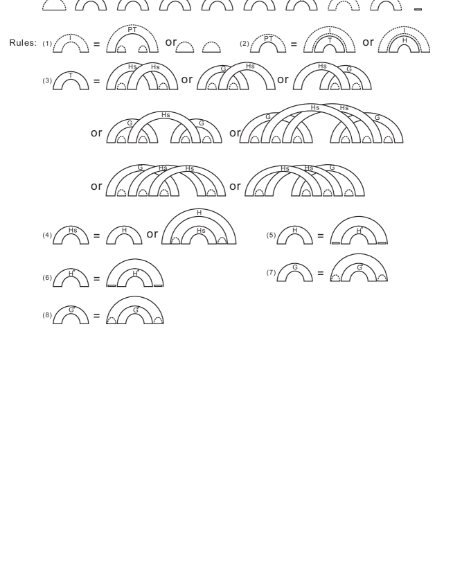
Now we are in position to formulate the production rules of ,
detailed in Figure 13:
(1): given an arbitrary structure , we remove starting
from and secondary structure blocks until an exterior arc is
encountered; such an exterior arc is contained in a pre-tight structure and
otherwise, contains no exterior arc and thus decomposes into
two disjoint secondary structures;
(2): the decomposition of pre-tight structures : if
is an exterior arc, then it is decomposed into a hybrid
and an arbitrary substructure ;
otherwise, it is decomposed into a tight structure and an
arbitrary structure ;
(3): in case of tight structures depending on which type of shadow is
contained in the tight structure, there are ways to disect into maximal
gap structures and hybrid-structures (which in turn collapses into interior
and exterior arcs of the irreducible shadow, respectively),
as well as secondary structures;
(4): a substructure consists of hybrids and secondary
structures, where each hybrid structure is maximal.;
(5): a maximal hybrid structure is decomposed into an
exterior arc and a non-maximal hybrid structure
with and ;
(6): a non-maximal hybrid structure is decomposed
into an exterior arc and a non-maximal hybrid structure
with and .;
(7): a maximal gap structure is decomposed via the
context-free grammar for secondary structures assuming that there is a
virtual hairpin loop in ; note that the substructure decomposed by a
maximal gap structure is no longer maximal; we use to
denote such a non-maximal gap structure derived via this decomposition;
(8): a non-maximal gap structure is decomposed similarly to
the decomposition of a maximal gap structure.
Lemma 2.
Any -structure over two backbones can uniquely be decomposed via , and any diagram generated by is a -structure over two backbones.
Proof.
First, we show that a -structure can uniquely be decomposed into blocks
containing exclusively non-crossing arcs. We shall establish this by induction
on the number of its irreducible shadows.
Induction basis: any -structure over two backbones that contains no
shadow of genus zero over two backbones exhibits no crossing arcs. Namely, it
contains only blocks that are either secondary structures or hybrids.
Accordingly, such a structure can be decomposed uniquely via the context-free
grammar of secondary structures or the unique decomposition of
hybrid-structures.
Induction step:
Suppose is a -structure containing irreducible shadows
over two backbones of genus .
We decompose from “inside to outside”, i.e., from the -end of and
the -end of . Suppose we encounter a substructure which collapses
into an irreducible shadow over two backbones of genus .
itself determines a unique maximal tight structure, , such that
. Removing from yields a diagram over two backbones
containing irreducible shadows over two backbones of genus
. The induction hypothesis guarantees the unique decomposition of
via .
It remains to show how to decompose tight structures: the shadow
of a tight structure is by construction irreducible and is given by one of the seven
irreducible shadows over two backbones described in Corollary 2.
In order to decompose a tight structure, we dissect it into maximal gap
structures and hybrid-structures (which in turn collapse into interior and
exterior arcs of the irreducible shadow, respectively), as well as secondary
structures.
All of these elements are -blocks that do not contain any
crossing arcs and can therefore be decomposed via a modified version of the
context-free grammar of secondary structures, described above.
Accordingly, there are seven ways to uniquely decompose a tight structure
into blocks containing exclusively non-crossing arcs.
Finally, we show that generates only -structures.
By construction, constructs tight structures via secondary
structure blocks, gap-structures and hybrid-structures. It furthermore
generates via the insertion of secondary structure blocks, hybrid structures
and tight structures. Thus, any structure generated by is a
-structure, whence the lemma.
∎
Theorem 2.
The grammar has the following properties:
(a) is unambiguous;
(b) allows computation of the partition function, base pairing
probabilities, the probability of hybrid-blocks, gap-structures and
Boltzmann sampling of -structures,
(c) has a time and space complexity
for generating the partition function of -structures.
Proof.
Assertion (a) follows from Lemma 2. Consequently, can be employed to count -interaction structures over two backbones for given sequences and as well as to compute the partition function
of -structures, where is the universal gas constant, is the temperature, is energy of structure over sequence , and is the set of -interaction structures in which all base pairs satisfy the base pairing rules for RNA, i.e., .
As for assertion (b), let denote the substructure represented by the nonterminal symbol in over and , where . Note that secondary structures are presented by an arbitrary structure setting one backbone empty. For each of these symbols, we introduce corresponding partial partition functions . Since is unambiguous, the recursions for the partial partition functions are derived by replacing minima by sums and addition of energy contribution by multiplication of partial partition functions, see e.g., Voß et al. (2006). For instance, the recursion for the partition functions corresponding to the nonterminal symbol reads
The probabilities of partial substructures of type are readily calculated from the partial partition functions. These “backward recursions” are analogous to those derived by McCaskill (1990) for secondary structures without crossings. It follows that we have
where the sum is over all -interaction structures containing .
Suppose is obtained by decomposing . The conditional probabilities are then given by , where represents the partition function of and represents the partition functions for those -configurations that contain . Taking the sum over all possible , we obtain
From this backward recursion, one immediately derives a stochastic backtracing recursion from the probabilities of partial structures that generates a Boltzmann sample of -interaction structures; see Tacker et al. (1996); Ding and Lawrence (2003); Huang et al. (2010) for similar constructions. The basic data structure for this sampling is a stack which stores blocks of the form , presenting interaction substructures of nonterminal symbols . is a set of base pairs storing those removed by the decomposition step in the grammar. We initialize with the block in , and . In each step, we pick up one element in and decompose it via the grammar with probability , where is the partition function of the block which is picked up from , and is the partition function of the target block which is decomposed by the rewriting rule. The base pairs which are removed in the decomposition step are moved to . For instance for the decomposition rule of , decomposing block into the two blocks: and , for fixed indices , , the probability of decomposing reads
The sampling step is iterated until is empty. The resulting -interaction structure is given by the list of base pairs. The probability of hybrid-structures can be calculated since a hybrid structure is by construction a block in the grammar, see Huang et al. (2010). The probability of interactions involving a fixed interval is given by
A gap structure, representing a maximal non-crossing stem on either backbone is also a -block, whence its probability is readily computable. Similarly, the probability of parings within the same backbone for a fixed interval can be expressed as:
In order to prove assertion (c), we observe that any product of two blocks has time complexity. We conclude from this that all -rules, except for (3) and (4) are of time complexity. It thus remains to analyze (3) and (4)333which are in fact for (3) and for (4) time complexity as it stands. To this end, we introduce intermediate blocks whose function is transitional storage.
-
1.
stores the result of the product and two secondary structure over interval and with and .
-
2.
stores the result of the product and two secondary structure over interval and with and .
-
3.
stores the result of the product and with .
-
4.
stores the result of the product and with and .
-
5.
stores the result of the product and with .
By virtue of these new blocks, we may rewrite (3) and (4) in terms of (3’) and (4’) as displayed in Figure 14.

After including these five intermediate blocks, we obtain two additional, nonterminal symbols in each decomposition rule. Since it requires two free variables to have the product of two nonterminal symbols and at most four variables to describe the two blocks, the decompositions in this form are of time complexity. We use at most -dimensional matrices to store the blocks in , whence the space complexity. ∎
7. Discussion
In this paper, we have introduced the toplogical filtration of RNA interaction structures and developed the notions of shadows, irreducibility and -structures for them. Shadows are of particular importance for the minimum free energy folding since they represent the basic motifs of genus . Since we have proved that for any genus there are always finitely many such shadows, it is therefore in principle possible to assign them individual energies, which would presumably lead to high specificity.
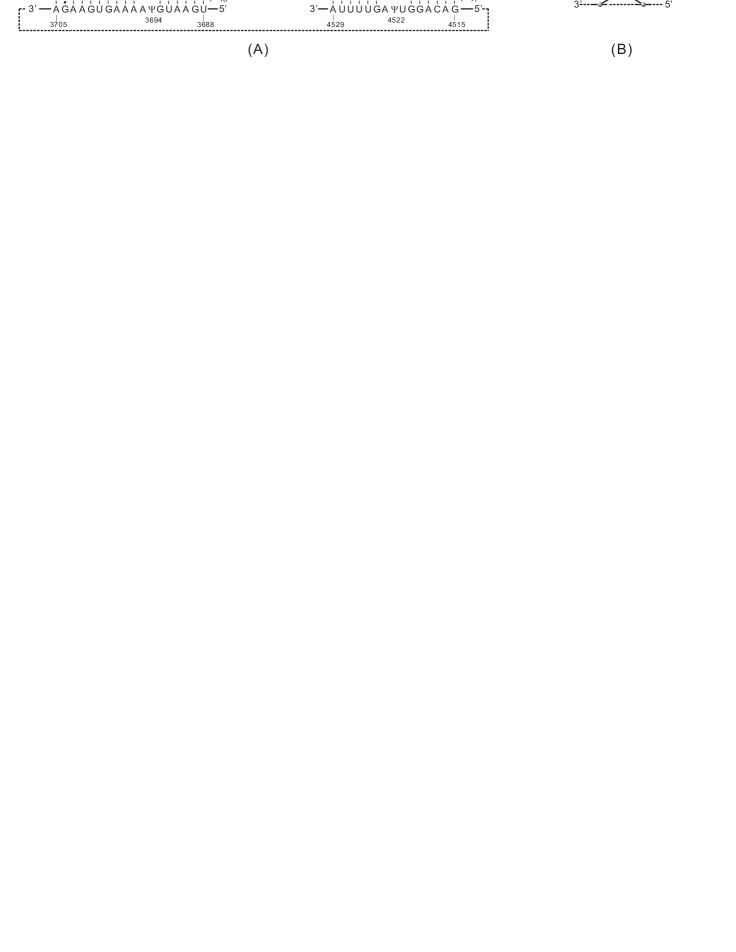
The simplest topological class of RNA interaction structures is that of -structures over two backbones. This is the two-backbone analogue of the classical RNA secondary structures. Despite their simple irreducible shadows (Corollary 2), -structures over two backbones exhibit features not present in the AP-structures of Pervouchine (2004); Alkan et al. (2006). Namely, they allow for pseudoknots formed by exterior arcs as reported, for instance, in Homo sapiens ACA27 snoRNA, see Figure 3 and Figure 15.
Let us next compare AP-structures and -structures over two backbones in more detail. Recall that an AP-structure, , is a graph such that
-
(1)
, are secondary structures,
-
(2)
is a set of exterior arcs without external pseudoknots,
-
(3)
contains no zig-zags.
A tight AP-structure () is a substructure that cannot be decomposed via block decomposition Huang et al. (2009, 2010). Accordingly, the shadow of a is connected and hence irreducibile. and tight structures of -structures over two backbones are distinct concepts. We have already observed that -structures over two backbones are not contained in the set of AP-structures. Likewise, AP-structures are not contained in the set of -structures over two backbones, for example, consider a shadow of a -structure over two backbones which consist of distinct, irreducible shadows over two backbones having genus . According to Lemma. 1, the genus of this diagram is . Drawing an interior arc covering the -endpoints of these shadows tightly, the resulting diagram is by construction a as in Figure 15. As inserting a single arc changes the genus at most by one, the diagram, , has genus , has an irreducible shadow and is consequently not a -structure over two backbones.

References
- Alkan et al. (2006) Alkan, C., Karakoc, E., Nadeau, J. H., et al. (2006). RNA-RNA interaction prediction and antisense RNA target search. J. Comput. Biol., 13, 267–282.
- Andronescu et al. (2005) Andronescu, M., Zhang, Z. C., and Condon, A. (2005). Secondary structure prediction of interacting RNA molecules. J. Mol. Biol., 345, 1101–1112.
- Bachellerie et al. (2002) Bachellerie, J. P., Cavaillé, J., and Hüttenhofer, A. (2002). The expanding snoRNA world. Biochimie, 84, 775–790.
- Banerjee and Slack (2002) Banerjee, D. and Slack, F. (2002). Control of developmental timing by small temporal RNAs: a paradigm for RNA-mediated regulation of gene expression. Bioessays, 24, 119–129.
- Benne (1992) Benne, R. (1992). RNA editing in trypanosomes. the use of guide RNAs. Mol. Biol. Rep., 16, 217–227.
- Bernhart et al. (2006) Bernhart, S., Tafer, H., Mückstein, U., et al. (2006). Partition function and base pairing probabilities of RNA heterodimers. Algorithms Mol. Biol., 1, 3.
- Bon et al. (2008) Bon, M., Vernizzi, G., Orland, H., et al. (2008). Topological classification of RNA structures. J. Mol. Biol., 379, 900–911.
- Busch et al. (2008) Busch, A., Richter, A. S., and Backofen, R. (2008). IntaRNA: efficient prediction of bacterial sRNA targets incorporating target site accessibility and seed regions. Bioinformatics, 24, 2849–2856.
- Chitsaz et al. (2009a) Chitsaz, H., Backofen, R., and Sahinalp, S. C. (2009a). biRNA: Fast RNA-RNA binding sites prediction. In Proceedings of the 9th Workshop on Algorithms in Bioinformatics (WABI), volume 5724 of LNCS, pages 25–36. Springer.
- Chitsaz et al. (2009b) Chitsaz, H., Salari, R., Sahinalp, S. C., et al. (2009b). A partition function algorithm for interacting nucleic acid strands. Bioinformatics, 25, i365–i373.
- Ding and Lawrence (2003) Ding, Y. and Lawrence, C. E. (2003). A statistical sampling algorithm for RNA secondary structure prediction. Nucleic Acid Res., 31, 7280–7301.
- Dirks et al. (2007) Dirks, R. M., Bois, J. S., Schaeffer, J. M., et al. (2007). Thermodynamic analysis of interacting nucleic acid strands. SIAM Review, 49, 65–88.
- Dowell and Eddy (2004) Dowell, R. D. and Eddy, S. R. (2004). Evaluation of several lightweight stochastic context-free grammars for RNA secondary structure prediction. BMC Bioinformatics, 5, 7.
- Hackermüller et al. (2005) Hackermüller, J., Meisner, N. C., Auer, M., et al. (2005). The effect of RNA secondary structures on RNA-ligand binding and the modifier RNA mechanism: a quantitative model. Gene, 345, 3–12.
- Hofacker et al. (1994) Hofacker, I. L., Fontana, W., Stadler, P. F., et al. (1994). Fast folding and comparison of RNA secondary structures. Monatsh. Chem., 125, 167–188.
- Huang et al. (2009) Huang, F. W. D., Qin, J., Reidys, C. M., et al. (2009). Partition function and base pairing probabilities for RNA-RNA interaction prediction. Bioinformatics, 25(20), 2646–2654.
- Huang et al. (2010) Huang, F. W. D., Qin, J., Reidys, C. M., et al. (2010). Target prediction and a statistical sampling algorithm for RNA-RNA interaction. Bioinformatics, 26, 175–181.
- Kiss et al. (2004) Kiss, A. M., Jady, B. E., Bertrand, E., et al. (2004). Human box H/ACA pseudouridylation guide RNA machinery. Mol. Cell .Biol., 24, 5797–5807.
- Kleitman (1970) Kleitman, D. (1970). Proportions of irreducible diagrams. Studies in Appl. Math., 49, 297–299.
- Kugel and Goodrich (2007) Kugel, J. and Goodrich, J. (2007). An RNA transcriptional regulator templates its own regulatory RNA. Nat. Struct. Mol. Biol., 3, 89–90.
- Ly et al. (2003) Ly, H., Xu, L., Rivera, M. A., et al. (2003). A role for a novel ‘trans-pseudoknot’ RNA-RNA interaction in the functional dimerization of human telomerase. Genes & Dev., 17, 1078–1083.
- Majdalani et al. (2002) Majdalani, N., Hernandez, D., and Gottesman, S. (2002). Regulation and mode of action of the second small RNA activator of RpoS translation, RprA. Mol. Microbiol., 46, 813–826.
- Massey (1967) Massey, W. S. (1967). Algebraic Topology: An Introduction. Springer-Veriag, New York.
- McCaskill (1990) McCaskill, J. S. (1990). The equilibrium partition function and base pair binding probabilities for RNA secondary structure. Biopolymers, 29, 1105–1119.
- McManus and Sharp (2002) McManus, M. T. and Sharp, P. A. (2002). Gene silencing in mammals by small interfering RNAs. Nature Reviews, 3, 737–747.
- Meisner et al. (2004) Meisner, N. C., Hackermüller, J., Uhl, V., et al. (2004). mRNA openers and closers: modulating AU-rich element-controlled mRNA stability by a molecular switch in mRNA secondary structure. Chembiochem., 5, 1432–1447.
- Mückstein et al. (2006) Mückstein, U., Tafer, H., Hackermüller, J., et al. (2006). Thermodynamics of RNA-RNA binding. Bioinformatics, 22, 1177–1182.
- Mückstein et al. (2008) Mückstein, U., Tafer, H., Bernhard, S. H., et al. (2008). Translational control by RNA-RNA interaction: Improved computation of RNA-RNA binding thermodynamics. In M. Elloumi, J. Küng, M. Linial, R. F. Murphy, K. Schneider, and C. T. Toma, editors, BioInformatics Research and Development — BIRD 2008, volume 13 of Comm. Comp. Inf. Sci., pages 114–127, Berlin. Springer.
- Narberhaus and Vogel (2007) Narberhaus, F. and Vogel, J. (2007). Sensory and regulatory RNAs in prokaryotes: A new german research focus. RNA Biol., 4, 160–164.
- Nussinov et al. (1978) Nussinov, R., Pieczenik, G., R., and Kleitman, D. J. (1978). Algorithms for loop matchings. SIAM J. of Appl. Math., 35, 68–82.
- Ofengand and Bakin (1997) Ofengand, J. and Bakin, A. (1997). Mapping to nucleotide resolution of pseudouridine residues in large subunit ribosomal RNAs from representative eukaryotes, prokaryotes, archaebacteria, mitochondria and chloroplasts. J. Mol. Biol., 266, 246–268.
- Orland and Zee (2002) Orland, H. and Zee, A. (2002). RNA folding and large matrix theory. Nuclear Physics B, 620, 456–476.
- Penner (2004) Penner, R. C. (2004). Cell decomposition and compactification of Riemann’s moduli space in decorated Teichmüller theory. In N. Tongring and R. C. Penner, editors, Woods Hole Mathematics-perspectives in math and physics, pages 263–301. World Scientific, Singapore. arXiv: math. GT/0306190.
- Penner (2011) Penner, R. C. (2011). Decorated Teichmüller Theory. European Mathematical Society, Zürich.
- Penner et al. (2010) Penner, R. C., Knudsen, M., Wiuf, C., and Andersen, J. E. (2010). Fatgraph models of proteins. Comm. Pure Appl. Math., 63, 1249–1297.
- Pervouchine (2004) Pervouchine, D. D. (2004). IRIS: Intermolecular RNA interaction search. Proc. Genome Informatics, 15, 92–101.
- Qin and Reidys (2007) Qin, J. and Reidys, C. M. (2007). A combinatorial framework for RNA tertiary interaction. Technical Report 0710.3523, arXiv. http://arxiv.org/abs/0710.3523.
- Rehmsmeier et al. (2004) Rehmsmeier, M., Steffen, P., Höchsmann, M., et al. (2004). Fast and effective prediction of microRNA/target duplexes. Gene, 10, 1507–1517.
- Reidys et al. (2010) Reidys, C. M., R., W. R., and Y., Z. A. Y. (2010). Modular, k-noncrossing diagrams. Electron. J. Comb., 17(1), R76.
- Reidys et al. (2011) Reidys, C. M., Huang, F. W. D., Andersen, J. E., et al. (2011). Topology and prediction of RNA pseudoknots. Bioinformatics, 27, 1076–1085.
- Rivas and Eddy (1999) Rivas, E. and Eddy, S. R. (1999). A dynamic programming algorithms for RNA structure prediction including pseudoknots. J. Mol. Biol., 285, 2053–2068.
- Salari et al. (2009) Salari, R., Backofen, R., and Sahinalp, S. C. (2009). Fast prediction of RNA-RNA interaction. In Proceedings of the 9th Workshop on Algorithms in Bioinformatics (WABI), volume 5724 of LNCS, pages 261–272. Springer.
- Sharma et al. (2007) Sharma, C. M., Darfeuille, F., Plantinga, T. H., et al. (2007). A small RNA regulates multiple ABC transporter mRNAs by targeting C/A-rich elements inside and upstream of ribosome-binding sites. Genes & Dev., 21, 2804–2817.
- Tacker et al. (1996) Tacker, M., Stadler, P. F., Bornberg-Bauer, E. G., et al. (1996). Algorithm independent properties of RNA structure prediction. Eur. Biophy. J., 25, 115–130.
- Tafer et al. (2009) Tafer, H., Kehr, S., Hertel, J., et al. (2009). RNAsnoop: Efficient target prediction for box H/ACA snoRNAs. Bioinformatics. in revision.
- Voß et al. (2006) Voß, B., Giegerich, R., and Rehmsmeier, M. (2006). Complete probabilistic analysis of RNA shapes. BMC Biology, 4, 5.
- Waterman (1979) Waterman, M. S. (1979). Combinatorics of RNA hairpins and cloverleaves. Stud. Appl. Math., 60, 91–96.
- Waterman and Smith (1978) Waterman, M. S. and Smith, T. F. (1978). RNA secondary structure: A complete mathematical analysis. Math. Biosci, 42, 257–266.
- Zagier (1995) Zagier, D. (1995). On the distribution of the number of cycles of elements in symmetric groups. Nieuw Arch. Wisk. IV, 13, 489–495.
- Zuker and Sankoff (1984) Zuker, M. and Sankoff, D. (1984). RNA secondary structures and their prediction. Bull. Math. Biol., 46, 591–621.