Smooth Solutions and Discrete Imaginary Mass
of the Klein-Gordon Equation in the de Sitter Background

Abstract

Using methods in the theory of semisimple Lie algebras, we can obtain all smooth solutions of the Klein-Gordon equation on the 4-dimensional de Sitter spacetime ($dS^{4}$). The mass of a Klein-Gordon scalar on $dS^{4}$ is related to an eigenvalue of the Casimir operator of $\mathfrak{so}(1,4)$. Thus it is discrete, or quantized. Furthermore, the mass $m$ of a Klein-Gordon scalar on $dS^{4}$ is imaginary: $m^{2}\propto-N(N+3)$, with $N\geqslant 0$ an integer.

1 Introduction

Ever since 1900, quantum theories (quantum mechanics and quantum field theory) and the theories of relativity (special and general relativity) are the most significant achievements in physics. However, for more than 100 years, the compatiblity of these two categories of theories is still a problem. Needless to say the conflict in spirit, only the obstacle in technique passing from general relativity to quantum theory has been enough problematic.

In the process of seeking for a theory of quantum gravity, there is the effort to establish QFT in curved spacetime[1, 2, 3, 4, 5, 6], assuming that the gravitational fields are dominated by a classical theory (typically by general relativity). The classical background may or may not be affected by the quantum fields. Currently the QFT in curved spacetime is mainly a framework generalized from the QFT in the Minkowski spacetime. Difference between a generic curved spacetime and the Minkowski spacetime has been considered, but, without much detailed knowledge of classical solutions of field theories in curved spacetime, some key points in QFT in curved spacetimes are inevitable questionable.

For a similar example, let us examine what happens when we consider scalar fields in $(1+1)$-dimensional toy spacetimes. If the spacetime is a Minkowski spacetime, scalar fields on it can be analyzed using the Fourier transform with respect to the spatial direction. If the space is closed as the circle $S^{1}$, however, scalar fields turn out to be Fourier series with respect to the spatial direction. In such an example, we can see how the difference of topologies could make great influence on the analysis tools.

Given a curved spacetime, its topological structure and geometric structure may affect many aspects of the fields. For a linear field equation, for instance, whether its solution space is infinite dimensional, whether some parameters (such as the mass) of the field equations are restricted to take only some special values, and so on, all depend on these structures. The QFT in curved spacetime must take these aspects into account.

In this paper, we take the Klein-Gordon equation on the 4-dimensional de Sitter spacetime (denoted by $dS^{4}$ in this paper) as an example. Applying the representation theory of semisimple Lie algebras, we can obtain all smooth classical solutions of the Klein-Gordon equation on $dS^{4}$. It is clear that, unlike the case of the Minkowski spacetime, the solution space of the K-G equation on $dS^{4}$ is finite dimensional. What’s more important is that the mass of a Klein-Gordon equation on $dS^{4}$ cannot be continuously real-valued. In fact, there exists nonzero solutions when and only when the mass $m$ satisfies

$$m^{2}=-N(N+3)\,\frac{\hbar^{2}}{c^{2}l^{2}}$$ (1)

for certain a nonnegative integer $N$, with $l$ the “radius” of $dS^{4}$. In the quantization process, the negative sign in $m^{2}$ should be a great obstacle to interpret $m$ to be the mass of particles excited by quantum scalar fields.

This paper is organized as follows. In Section 2 we outline our idea of how to obtain all smooth solutions of the Klein-Gordon equation on $dS^{4}$. We start the outline from the well know theory of angular momentum in quantum mechanics. In Section 3 we describe the whole principle and program of our method. In Section 4 we apply the theory of semisimple Lie algebras to $\mathfrak{so}(1,4)\otimes_{\mathbb{R}}\mathbb{C}$, the complexification of $\mathfrak{so}(1,4)$, and describe its algebraic structures which have nothing to do with its representations. For convenience $\mathfrak{so}(1,4)\otimes_{\mathbb{R}}\mathbb{C}$ is denoted by $\mathfrak{L}$. In Section 5 we apply the representation theory of semisimple Lie algebras to the $\mathfrak{L}$-module $C^{\infty}(dS^{4})$, analogous to the coordinate representation of angular momentum operators in quantum mechanics. In this section we give some coordinate systems adapted to the Cartan subalgebras of $\mathfrak{L}$, and construct irreducible $\mathfrak{L}$-submodules of $C^{\infty}(dS^{4})$. In Section 6 we give the mass of the Klein-Gordon equation and its smooth solutions. Then, finally, in Section 7, we give the summary and discuss some related problems. Detailed investigation and proofs are left in the appendices.

2 Outline of the Ideas

In general relativity, the Klein-Gordon equation reads

$$g^{ab}\nabla_{a}\nabla_{b}\phi+\frac{m^{2}c^{2}}{\hbar^{2}}\,\phi=0\,,$$ (2)

where $\nabla_{a}$ is the Levi-Civita connection. (Indices like $a$ and $b$ are abstract indices [7].) In this paper the signature of the metric tensor field $g_{ab}$ is like that of

$$(\eta_{\mu\nu})_{4\times 4}=\mathrm{diag}(1,-1,-1,-1)\,.$$ (3)

The Klein-Gordon equation is a linear PDE. To solve a PDE, one often applies the method of separation of variables. However, whether this method works depends heavily on the choice of the coordinates $x^{\mu}$. If one is not so lucky to choose the right coordinates, this method would fail even if the PDE can be easily solved in certain a right coordinate system.

In order to solve a linear PDE using the method of separation of variables, we must choose a coordinate system that is closely related to the symmetry of the PDE. When the symmetry group is a Lie group with a sufficient large rank (the dimension of its Cartan subgroup), it is even possible to solve the PDE by virtue of the theory of Lie groups and Lie algebras. In this case the method of separation of variables is only needed to find out a maximal vector[8] corresponding to the highest weight. After the maximal vectors have been found out, the solution space of the PDE can be easily, but often tediously, constructed.

To show this, we take the equation

$$h^{\alpha\beta}D_{\alpha}D_{\beta}Y=-\lambda Y$$ (4)

on $S^{2}$ (the unit 2-sphere) as an example, where $D_{\alpha}$ is the Levi-Civita connection compatible with the standard metric tensor field $h_{\alpha\beta}$ on $S^{2}$. This is the eigenvalue equation of the Laplacian operator for 0-forms on $S^{2}$. Since the symmetry group of $S^{2}$ is $O(3,\mathbb{R})$, and since eq. (4) is determined by the metric tensor field $h_{\alpha\beta}$, the symmetry group of eq. (4) contains $O(3,\mathbb{R})$ as a Lie subgroup. In the spherical coordinate system $(\theta,\varphi)$, eq. (4) takes the well known form

$$\frac{1}{\sin\theta}\,\frac{\partial}{\partial\theta}\Big{(}\sin\theta\frac{\partial Y}{\partial\theta}\Big{)}+\frac{1}{\sin^{2}\theta}\,\frac{\partial^{2}Y}{\partial\varphi}=-\lambda\,Y\,.$$ (5)

On the one hand, this PDE arises from the Helmholtz equation by separation of variable, and a further separation of variable leads to the general Legendre equation, together with the equation of a simple harmonic oscillator with respect to the variable $\varphi$. As a result, the solution of eq. (5), namely, eq. (4), is a linear combination

$$Y=\sum_{m=-l}^{l}C_{m}\,Y_{lm}(\theta,\varphi)$$ (6)

of spherical harmonics $Y_{lm}(\theta,\varphi)$ with a fixed nonnegative integer $l$, where $C_{m}$ are arbitrary constants, and $\lambda=l(l+1)$.

On the other hand, in quantum mechanics, there is a more elegant method using the theory of angular momentum operators to solve eq. (5). In geometry, the angular momentum operators $\hat{\boldsymbol{L}}=\boldsymbol{r}\times\hat{\boldsymbol{p}}=-i\hbar\,\boldsymbol{r}\times\nabla$ are proportional to three Killing vector fields

$$I_{x} =\frac{1}{i\hbar}\,\hat{L}_{x}=\sin\varphi\,\frac{\partial}{\partial\theta}+\cot\theta\cos\varphi\,\frac{\partial}{\partial\varphi}\,,$$ (7)

$$I_{y} =\frac{1}{i\hbar}\,\hat{L}_{y}=-\cos\varphi\,\frac{\partial}{\partial\theta}+\cot\theta\sin\varphi\,\frac{\partial}{\partial\varphi}\,,$$ (8)

$$I_{z} =\frac{1}{i\hbar}\,\hat{L}_{z}=-\frac{\partial}{\partial\varphi}\,,$$ (9)

respectively. To apply the theory of angular momentum operators to the coordinate representation is, in fact, equivalent to apply the representation theory of $\mathfrak{so}(3,\mathbb{R})$ to $C^{\infty}(S^{2})$, the $\mathfrak{so}(3,\mathbb{R})$-module of all smooth functions on $S^{2}$. In this manner $Y_{ll}(\theta,\varphi)$, which acts as the maximal vector in the representation theory, can be obtained by solving two PDEs of order one:

$$\hat{L}_{z}Y_{ll}=l\hbar\,Y_{ll}\,,\qquad\hat{L}_{+}Y_{ll}=0\,.$$

Then all other $Y_{lm}(\theta,\varphi)$ can be obtained from

$$\hat{L}_{-}Y_{lm}=\hbar\sqrt{(l+m)(l-m+1)}\,Y_{l,m-1}$$

for $m=l$, $l-1$, …, $-l$ recursively. It is well known that eq. (5), namely, eq. (4), is equivalent to

$$\hat{\boldsymbol{L}}^{2}Y=\lambda\hbar^{2}\,Y\,,$$

and $\hat{\boldsymbol{L}}^{2}$ is a Casimir operator of $\mathfrak{so}(3,\mathbb{R})$. Because all $Y_{lm}$ with $m=l$, $l-1$, …, $-l$ span an irreducible $\mathfrak{so}(3,\mathbb{R})$-module, the linear combination (6) is automatically a solution of the above equation, according to Schur’s lemma [8]. In order to determine the value of $\lambda$, we need simply substitute $Y=Y_{ll}$ into the above equation, obtaining $\lambda=l(l+1)$.

The reason that separation of variables works is deeply related to the fact that the $\varphi$-coordinate curves are integral curves of $\hat{L}_{z}$, which can be easily seen from eq. (9). Note that $\hat{L}_{z}$ spans a Cartan subalgebra of $\mathfrak{so}(3,\mathbb{R})$, and that each $Y_{lm}$ spans a weight space with respect to this Cartan subalgebra.

The above approach is very instructive. Since the de Sitter spacetime and anti-de Sitter spacetime are maximally symmetric, such an approach can be easily applied to field equations in de Sitter or anti-de Sitter backgrounds.

In this paper we only take the Klein-Gordon equation on $dS^{4}$, the 4-dimensional de Sitter spacetime (as a background), as an example. The main idea can be illustrated as follows.

The symmetry group of $dS^{4}$ is $O(1,4)$, whose Lie algebra $\mathfrak{so}(1,4)$ induces a Lie algebra of Killing vector fields on $dS^{4}$. Via these Killing vector fields, $\mathfrak{so}(1,4)$ acts on smooth functions on $dS^{4}$. Thus $C^{\infty}(dS^{4})$, the space of all smooth functions on $dS^{4}$, is an $\mathfrak{so}(1,4)$-module. (Equivalently speaking, $C^{\infty}(dS^{4})$ is a representation space of $\mathfrak{so}(1,4)$.) Since the Klein-Gordon equation on $dS^{4}$ is $O(1,4)$-invariant, its solution space $\mathscr{S}_{\textrm{KG}}(dS^{4})$ is $O(1,4)$-invariant. Hence $\mathscr{S}_{\textrm{KG}}(dS^{4})$ is an $\mathfrak{so}(1,4)$-submodule of $C^{\infty}(dS^{4})$. It must be the direct sum of some irreducible $\mathfrak{so}(1,4)$-submodules. Therefore, to obtain the solution space of the Klein-Gordon equation on $dS^{4}$, we must construct these irreducible $\mathfrak{so}(1,4)$-submodules of $C^{\infty}(dS^{4})$.

There is an important fact: the Klein-Gordon equation on $dS^{4}$ is, in fact, an eigenvalue equation of the Casimir element of $\mathfrak{so}(1,4)$. See, eq. (19) in this paper. By aid of this fact, it is very easy to obtain all smooth solutions of the Klein-Gordon equation in the de Sitter background. An interesting and important consequence is that the mass in the Klein-Gordon equation is discrete and imaginary, as shown in eq. (1).

3 Symmetry Group and Solution Space of the Klein-Gordon Equation on the de Sitter Spacetime

3.1 Symmetry Group of the de Sitter Spacetime

Now we consider the 5-dimensional Minkowski space $\mathbb{R}^{1,4}$, with $\xi^{A}$ ($A=0$, $1$, …, $4$) the Minkowski coordinates on it. The de Sitter spacetime of radius $l>0$ can be treated as the hypersurface

$$\eta_{AB}\,\xi^{A}\xi^{B}=-l^{2}$$ (10)

of $\mathbb{R}^{1,4}$, where $(\eta_{AB})_{5\times 5}=\mathrm{diag}(1,-1,\dots,-1)$. The linear group $O(1,4)$ is the symmetry group of $\mathbb{R}^{1,4}$, leaving both the line element $\mathrm{d}s^{2}=\eta_{AB}\,\mathrm{d}\xi^{A}\,\mathrm{d}\xi^{B}$ of $\mathbb{R}^{1,4}$ and the hypersurface (10) invariant. Consequently, $O(1,4)$ is also the symmetry group of $dS^{4}$.

For later usage, we describe the symmetries of $dS^{4}$ in some details. The metric tensor field $\widetilde{\boldsymbol{\eta}}:=\eta_{AB}\,\mathrm{d}\xi^{A}\otimes\mathrm{d}\xi^{B}$ on $\mathbb{R}^{1,4}$ induces a metric tensor field $\mathbf{g}$ on $dS^{4}$. In fact, let $i\colon dS^{4}\hookrightarrow\mathbb{R}^{1,4}$ be the inclusion, then $\mathbf{g}=i^{*}\widetilde{\boldsymbol{\eta}}$ is the pullback of $\tilde{\boldsymbol{\eta}}$. A linear transformation $D\in O(1,4)$ on $\mathbb{R}^{1,4}$ leaves $dS^{4}$, the hypersurface (10), invariant. Thus we may set the restriction of $D$ to $dS^{4}$, $\psi_{D}=D\big{|}_{dS^{4}}\colon dS^{4}\rightarrow dS^{4}$, to be a transformation on $dS^{4}$. It follows that $\psi_{D}$ is a symmetry of $(dS^{4},\mathbf{g})$. That is, $\psi_{D}$ is a diffeomorphism, satisfying

$$\psi_{D}^{*}\mathbf{g}=\mathbf{g}\,.$$ (11)

Obviously, all $\psi_{D}$ with $D\in O(1,4)$ form a group, which is isomorphic to $O(1,4)$.

In the following we describe the Lie algebras of the symmetry group.

First, there are the $5\times 5$ matrices $X_{AB}\in\mathfrak{so}(1,4)$ with $A$, $B=0$, $1$, …, $4$, whose $(C,D)^{\textrm{th}}$ entry reads

$$(X_{AB})^{C}_{D}=\delta^{C}_{A}\,\eta_{BD}-\delta^{C}_{B}\,\eta_{AD}\,.$$ (12)

They satisfy $X_{AB}=-X_{BA}$ and

$$[X_{AB},X_{CD}]=\eta_{BC}\,X_{AD}+\eta_{AD}\,X_{BC}-\eta_{AC}\,X_{BD}-\eta_{BD}\,X_{AC}\,.$$ (13)

Furthermore, all $X_{AB}$ with $A<B$ form a basis of $\mathfrak{so}(1,4)$.

According to the theory of Lie groups, through the action of $O(1,4)$ on $\mathbb{R}^{1,4}$, each matrix $X=(X^{A}_{B})\in\mathfrak{so}(1,4)$ generates a vector field

$$\widetilde{\mathbf{X}}:=-X^{A}_{B}\,\xi^{B}\,\frac{\partial}{\partial\xi^{A}}$$ (14)

on $\mathbb{R}^{1,4}$. Let $\mathfrak{X}(\mathbb{R}^{1,4})$ be the Lie algebra of smooth vector fields on $\mathbb{R}^{1,4}$. Then the map $\mathfrak{so}(1,4)\rightarrow\mathfrak{X}(\mathbb{R}^{1,4})$, $X\mapsto\tilde{\boldsymbol{X}}$ is a homomorphism of Lie algebras. Roughly speaking, the above $\widetilde{\mathbf{X}}$ is generated by the infinitesimal transformation corresponding to the matrix $-X$. In other words, the 1-parameter group of $\tilde{\mathbf{X}}$ equals to $\exp(-tX)\in O(1,4)$. So $\widetilde{\mathbf{X}}$ is a Killing vector field on $\mathbb{R}^{1,4}$, and vice versa, a Killing vector field on $\mathbb{R}^{1,4}$ corresponds to a matrix $X\in\mathfrak{so}(1,4)$ via eq. (14). For convenience, the Lie algebra consisting of all Killing vector fields on $\mathbb{R}^{1,4}$ will be denoted by $\mathfrak{K}(\mathbb{R}^{1,4})$. Then the map described in the above results in an isomorphism of Lie algebras from $\mathfrak{so}(1,4)$ to $\mathfrak{K}(\mathbb{R}^{1,4})$, mapping $[X,Y]$ for each pair of $X$, $Y\in\mathfrak{so}(1,4)$ to the commutator $[\widetilde{\mathbf{X}},\widetilde{\mathbf{Y}}]$ of the corresponding Killing vector fields $\widetilde{\mathbf{X}}$ and $\widetilde{\mathbf{Y}}$. Especially, the matrix $X_{AB}\in\mathfrak{so}(1,4)$, as defined in eq. (12), corresponds to the Killing vector field

$$\widetilde{\mathbf{X}}_{AB}=\xi_{A}\,\frac{\partial}{\partial\xi^{B}}-\xi_{B}\,\frac{\partial}{\partial\xi^{A}}\,,$$ (15)

where $\xi_{A}:=\eta_{AB}\,\xi^{B}$. Thus there are the commutators

$$[\widetilde{\mathbf{X}}_{AB},\widetilde{\mathbf{X}}_{CD}]=\eta_{BC}\,\widetilde{\mathbf{X}}_{AD}+\eta_{AD}\,\widetilde{\mathbf{X}}_{BC}-\eta_{AC}\,\widetilde{\mathbf{X}}_{BD}-\eta_{BD}\,\widetilde{\mathbf{X}}_{AC}\,.$$ (16)

In fact, the above equations can be directly verified by virtue of eq. (15).

For an $X\in\mathfrak{so}(1,4)$, the corresponding Killing vector field $\widetilde{\mathbf{X}}\in\mathfrak{K}(\mathbb{R}^{1,4})$ is tangent to $dS^{4}$ at any point $\xi\in dS^{4}$. Therefore such a vector field induces a vector field on $dS^{4}$, denoted by $\mathbf{X}$. Roughly speaking, $\mathbf{X}$ is the restriction of $\tilde{\mathbf{X}}$ (as a section of the tangent bundle of $\mathbb{R}^{1,4}$) to $dS^{4}$; strictly speaking, $\mathbf{X}$ is $i$-related[9] to $\tilde{\mathbf{X}}$, with $i\colon dS^{4}\hookrightarrow\mathbb{R}^{1,4}$ being the inclusion. In fact, if $X\in\mathfrak{so}(1,4)$ corresponds to $\widetilde{\mathbf{X}}$, the 1-parameter group $\psi_{\exp(-tX)}$ is just generated by the vector field $\mathbf{X}$. Hence, obviously, $\mathbf{X}$ is a Killing vector field on $dS^{4}$. It can be verified that a Killing vector field on $dS^{4}$ corresponds to a matrix in $\mathfrak{so}(1,4)$. In this way, there exists the isomorphism of Lie algebras from $\mathfrak{so}(1,4)$ to $\mathfrak{K}(dS^{4})$, where $\mathfrak{K}(dS^{4})$ consists of all Killing vector fields on $dS^{4}$. Especially, $X_{AB}$, hence $\widetilde{\mathbf{X}}_{AB}$, corresponds to a Killing vector field $\mathbf{X}_{AB}$ on $dS^{4}$, satisfying

$$[\mathbf{X}_{AB},\mathbf{X}_{CD}]=\eta_{BC}\,\mathbf{X}_{AD}+\eta_{AD}\,\mathbf{X}_{BC}-\eta_{AC}\,\mathbf{X}_{BD}-\eta_{BD}\,\mathbf{X}_{AC}\,.$$ (17)

3.2 Symmetries of the Klein-Gordon Equation on $dS^{4}$

The Klein-Gordon equation on $dS^{4}$ is as shown in eq. (2). Given a local coordinate system $(x^{\mu})$ in $dS^{4}$, the expression of $\mathbf{X}_{AB}$ might be quite complicated. Interestingly however, it can be proved that, for an arbitrary smooth function $\phi$ on $dS^{4}$,

$$g^{ab}\,\nabla_{a}\nabla_{b}\phi=-\frac{1}{2l^{2}}\,\eta^{AC}\eta^{BD}\,L_{\mathbf{X}_{AB}}L_{\mathbf{X}_{CD}}\phi\,,$$ (18)

where $L_{\mathbf{X}}$ is the Lie derivative with respect to a vector field $\mathbf{X}$. Therefore, the Klein-Gordon equation (2) is, indeed, an eigenvalue equation

$$C\phi=\frac{m^{2}c^{2}l^{2}}{\hbar^{2}}\,\phi$$ (19)

for the Casimir operator

$$C:=\frac{1}{2}\,\eta^{AC}\eta^{BD}\,L_{\mathbf{X}_{AB}}\,L_{\mathbf{X}_{CD}}$$ (20)

of the second order.

As mentioned in §3.1, an orthogonal transformation $D$ on $\mathbb{R}^{1,4}$ induces the automorphism $\psi_{D}$ of $(dS^{4},\mathbf{g})$, whose pullback further induces a transformation $\psi_{D}^{*}\colon C^{\infty}(dS^{4})\rightarrow C^{\infty}(dS^{4})$, mapping an arbitrary smooth function $\phi$ on $dS^{4}$ to another smooth function $\phi^{\prime}=\psi_{D}^{*}\phi:=\phi\circ\psi_{D}$. That is, at arbitrary point $\xi\in dS^{4}$,

$$\phi^{\prime}(\xi)=\phi(\psi_{D}(\xi))=\phi(D\xi)\,.$$ (21)

The group homomorphism mapping $D\in O(1,4)$ to $\psi_{D^{-1}}^{*}\in\mathrm{GL}(C^{\infty}(dS^{4}))$ is a representation of $O(1,4)$ on the vector space $C^{\infty}(dS^{4})$. In other words, we have an action of $O(1,4)$ on $C^{\infty}(dS^{4})$ on the left as follows: $O(1,4)\times C^{\infty}(dS^{4})\rightarrow C^{\infty}(dS^{4})$, $(D,\phi)\mapsto\psi_{D^{-1}}^{*}\phi$.

Since the Klein-Gordon equation (2) is determined by the metric tensor field $\mathbf{g}$, while $\psi_{D}^{*}$ leaves $\mathbf{g}$ invariant (see, eq. (11)), it follows that, if $\phi$ is a smooth solution of eq. (2), so is $\psi_{D}^{*}\phi$. Let $\mathscr{S}_{\textrm{KG}}(dS^{4})$ be the solution space of eq. (10), namey, the set consisting of all smooth solutions of eq. (2). Then $\mathscr{S}_{\textrm{KG}}(dS^{4})$ is a vector space over $\mathbb{R}$ (for real-valued functions) or $\mathbb{C}$ (for complex-valued functions), being invariant under $\psi_{D}^{*}$ for arbitrary $D\in O(1,4)$. In other words, the action of $O(1,4)$ on $C^{\infty}(dS^{4})$ can be restricted to be $O(1,4)\times\mathscr{S}_{\textrm{KG}}(dS^{4})\rightarrow\mathscr{S}_{\textrm{KG}}(dS^{4})$, $(D,\phi)\mapsto\psi_{D^{-1}}^{*}\phi$.

3.3 Smooth Solutions of the Klein-Gordon Equation on $dS^{4}$

For any smooth function $\phi$ on $dS^{4}$ and any $X\in\mathfrak{so}(1,4)$, the Lie derivative $L_{\mathbf{X}}\phi$ of $\phi$ with respect to $\mathbf{X}$ can be defined point-wisely [9] by the derivative of $\psi_{\exp(-\lambda X)}^{*}\phi$ with respect to the parameter $\lambda$, where the relation of $X$ and $\mathbf{X}$ is as described in §3.1. For any $X\in\mathfrak{so}(1,4)$ and any $\phi\in C^{\infty}(dS^{4})$, the action of $X$ upon $\phi$ results in $X.\phi$, defined by

$$X.\phi:=L_{\mathbf{X}}\phi=\mathbf{X}\phi\,.$$ (22)

Obviously, $X.\phi$ is still a smooth function on $dS^{4}$. Hence $C^{\infty}(dS^{4})$ becomes an $\mathfrak{so}(1,4)$-module.

Especially, if $\phi$ is a smooth solution of the Klein-Gordon equation (2), so is $X.\phi$ for any $X\in\mathfrak{so}(1,4)$. Thus $\mathscr{S}_{\textrm{KG}}(dS^{4})$ is an $\mathfrak{so}(1,4)$-submodule of $C^{\infty}(dS^{4})$.

In §4.1 we shall show that $\mathfrak{so}(1,4)$ is semisimple. According to the representation theory of Lie algebras [8], the solution space $\mathscr{S}_{\textrm{KG}}(dS^{4})$ can be decomposed into the direct sum of irreducible $\mathfrak{so}(1,4)$-submodules. Hence every solution $\phi$ of eq. (2) can be decomposed into the sum of finite many functions $\phi_{1}$, …, $\phi_{k}$, with $\phi_{i}$ ($i=1$, …, $k$) belonging to certain an irreducible $\mathfrak{so}(1,4)$-submodule.

Since eq. (19) is equivalent to eq. (2) and

$$[C,L_{\mathbf{X}}]=0\,,\qquad\forall\mathbf{X}\in\mathfrak{K}(dS^{4})\,,$$ (23)

it follows Schur’s lemma [8] that the solution space $\mathscr{S}_{\textrm{KG}}(dS^{4})$ is the direct sum of irreducible $\mathfrak{so}(1,4)$-submodules belonging to the same eigenvalue of $C$. In other words, any function $\phi$ belonging to an irreducible $\mathfrak{so}(1,4)$-submodule of $C^{\infty}(dS^{4})$ is a smooth solution of the Klein-Gordon equation (19) with certain a mass.

Therefore, in order to find smooth solutions of the Klein-Gordon equation on $dS^{4}$, it is necessary to find the irreducible $\mathfrak{so}(1,4)$-submodule of $C^{\infty}(dS^{4})$.

A consequence of the above conclusion is that the mass of the Klein-Gordon equation cannot be arbitrary. The mass must be related to an eigenvalue of $C$, which in turn is determined by the highest weights of irreducible $\mathfrak{so}(1,4)$-submodules contained in $\mathscr{S}_{\textrm{KG}}(dS^{4})$. In §6 we can calculate the mass, as shown in eq. (1), where the nonnegative integer $N$ specifies the highest weight of an irreducible $\mathfrak{so}(1,4)$-submodule. Furthermore, in §6 we shall prove that different highest weight (or equivalently, $N$) corresponds to different mass. It follows that the solution space $\mathscr{S}_{\textrm{KG}}(dS^{4})$ is nothing but an irreducible $\mathfrak{so}(1,4)$-submodule of $C^{\infty}(dS^{4})$.

4 Structure of the Lie Algebra $\mathfrak{so}(1,4)$

There are papers discussing irreducible representations of $\mathfrak{so}(1,4)$, such as [11] and [12]. In [11], unitary representations of $\mathfrak{so}(1,4)$ were constructed out of irreducible representations of $\mathfrak{so}(4,\mathbb{R})$, similar to the method by Wigner[13]. The resulted irreducible unitary representations are infinite dimensional[12]. Since we are seeking the solution space of the Klein-Gordon equation, in this paper we are not interested in the representation of $\mathfrak{so}(1,4)$, but rather its representation spaces, irreducible $\mathfrak{so}(1,4)$-submodules in $C^{\infty}(dS^{4})$. For this purpose, the framework in [11] is so complicated in practice.

In this paper we construct irreducible $\mathfrak{so}(1,4)$-submodules of $C^{\infty}(dS^{4})$ using the standard methods in the theory of Lie groups[9] and Lie algebras[8].

In this section we briefly describe the abstract structure of $\mathfrak{so}(1,4)$ and/or its complexification, $\mathfrak{L}=\mathfrak{so}(1,4)\otimes_{\mathbb{R}}\mathbb{C}$. In the next section we apply the representation theory to the $\mathfrak{so}(1,4)$-module $C^{\infty}(dS^{4})$.

4.1 The Killing Form of $\mathfrak{so}(1,4)$

In this paper, the Killing form of $\mathfrak{so}(1,4)$ is denoted by $\kappa$. It is easy to verify that

$$\kappa(X_{AB},X_{CD})=6\,(\eta_{AD}\,\eta_{BC}-\eta_{AC}\,\eta_{BD})\,.$$ (25)

This tells us that (1) for $X_{AB}$ with $A<B$, they are mutually orthogonal (with respect to the Killing form), and that (2) the Killing form of $X_{AB}$ with itself is $\mp 6$. A corollary is that the Killing form is nondegenerate. Hence $\mathfrak{so}(1,4)$ is a semisimple Lie algebra.

4.2 The Abstract Root System of $\mathfrak{L}=\mathfrak{so}(1,4)\otimes_{\mathbb{R}}\mathbb{C}$

According to the theory of Lie algebras, if a semisimple Lie algebra $\mathfrak{L}$ is over an algebraically closed field of characteristic 0, such as $\mathbb{C}$, the abstract root system $\Phi$ of $\mathfrak{L}$ is determined by $\mathfrak{L}$ itself. See, for example, §16 in [8]. However, since the Lie algebra $\mathfrak{so}(1,4)$ is over $\mathbb{R}$, which is not an algebraically closed field, the theory of root systems for semisimple Lie algebras cannot be applied to it. Therefore we use its complexification $\mathfrak{L}:=\mathfrak{so}(1,4)\otimes_{\mathbb{R}}\mathbb{C}$ instead.

All the following results can be obtained using the standard approach in the theory of Lie algebra[8]. We neglect all these processes, listing the results only.

The Dynkin diagram of $\mathfrak{L}$ is as shown in Figure 1.

Figure 1: The Dynkin diagram of $\mathfrak{L}=\mathfrak{so}(1,4)\otimes_{\mathbb{R}}\mathbb{C}$.

Therefore, $\mathfrak{L}$ is a semisimple Lie algebra of type $\mbox{{B}}_{2}$. Let $\Delta=\{\alpha_{1},\alpha_{2}\}$ be the base of the root system $\Phi$ of $\mathfrak{L}$. Then its Cartan matrix reads

$$\big{(}\langle\alpha_{i},\alpha_{j}\rangle\big{)}_{2\times 2}=\left(\begin{array}[]{rr}2&-2\\ -1&2\end{array}\right)\,.$$ (26)

Here the Cartan integer related to two roots $\alpha$ and $\beta$ is

$$\langle\alpha,\beta\rangle=\frac{2\,(\alpha,\beta)}{(\beta,\beta)}\,,$$ (27)

where $(\cdot,\cdot)$ is the inner product on the Euclidean space spanned by all the roots of $\mathfrak{L}$.

The root system $\Phi$ of $\mathfrak{L}$ consists of the following roots: $\pm\alpha_{1}$, $\pm\alpha_{2}$, $\pm(\alpha_{1}+\alpha_{2})$ and $\pm(\alpha_{1}+2\,\alpha_{2})$. For later reference the set of positive roots is denoted by $\Phi^{+}$, reading

$$\Phi^{+}=\{\alpha_{1},\ \alpha_{2},\alpha_{1}+\alpha_{2},\ \alpha_{1}+2\,\alpha_{2}\}\,.$$ (28)

Then $\Phi=\Phi^{+}\cup\Phi^{-}$, where $\Phi^{-}=-\Phi^{+}$ is the set of negative roots.

Let $E_{\Phi}$ be the 2-dimensional Euclidean space spanned by the root system $\Phi$. Obviously, $\alpha_{1}$ and $\alpha_{2}$ form a basis of $E_{\Phi}$. In this paper, the inner product on $E_{\Phi}$ is resulted in from the Killing form $\kappa$, as follows: We first choose a Cartan subalgebra $\mathfrak{h}$ of $\mathfrak{L}$. Then the restriction of $\kappa$ to $\mathfrak{h}$ is nondegenerate [8], inducing a nondegenerate bilinear form $(\cdot,\cdot)$ on $E_{\mathfrak{h}^{*}}$, satisfying

$$(\alpha_{1},\alpha_{1})=\frac{1}{3}\,,\qquad(\alpha_{1},\alpha_{2})=-\frac{1}{6}\,,\qquad(\alpha_{2},\alpha_{2})=\frac{1}{6}\,.$$ (29)

Then such a bilinear form is turned to be the inner product on $E_{\Phi}$. With the aid of the data in eqs. (29), the roots can be drawn as in Figure 2.

Figure 2: The root system of $\mathfrak{L}=\mathfrak{so}(1,4)\otimes_{\mathbb{R}}\mathbb{C}$.

The Cartan subalgebra (also a maximal toral subalgebra) of a semisimple Lie algebra is not unique. Being conjugate to each other [8], none of these Cartan subalgebras is more significant than others. However, when the action of the Lie algebra on a differential manifold is considered, this is no longer the same situation. So, for $\mathfrak{L}=\mathfrak{so}(1,4)\otimes_{\mathbb{R}}\mathbb{C}$, we shall take two typical Cartan subalgebras into account.

4.3 The Cartan Subalgebra and Root Spaces (I)

The first Cartan subalgebra is spanned by $X_{12}$ and $X_{04}$, and denoted by $\mathfrak{h}$ in this paper. With respect to $\mathfrak{h}$, the roots $\alpha_{1}$ and $\alpha_{2}\in\mathfrak{h}^{*}$ satisfy

$$\alpha_{1}(X_{12}) =i,\qquad \alpha_{1}(X_{04}) =-1,$$ (30)

$$\alpha_{2}(X_{12}) =0, \alpha_{2}(X_{04}) =1.$$ (31)

For each positive root $\beta\in\Phi^{+}$, the root spaces of $\beta$ and $-\beta$ are denoted by $\mathfrak{L}_{\pm\beta}$, respectively. The bases of $\mathfrak{L}_{\pm\beta}$ are denoted by $e_{\beta}$ and $f_{\beta}$, respectively. They are chosen as follows:

$$e_{\alpha_{1}} =\frac{1}{2}\,(X_{01}-i\,X_{02}-X_{14}+i\,X_{24})\,,\qquad f_{\alpha_{1}} =\frac{1}{2}\,(X_{01}+i\,X_{02}+X_{14}+i\,X_{24})\,,$$ (32)

$$e_{\alpha_{2}} =X_{03}+X_{34}\,, f_{\alpha_{2}} =X_{03}-X_{34}\,,$$ (33)

$$e_{\alpha_{1}+\alpha_{2}} =-X_{13}+i\,X_{23}\,, f_{\alpha_{1}+\alpha_{2}} =X_{13}+i\,X_{23}\,,$$ (34)

$$e_{\alpha_{1}+2\alpha_{2}} =-\frac{1}{2}\,(X_{01}-i\,X_{02}+X_{14}-i\,X_{24})\,,\quad f_{\alpha_{1}+2\alpha_{2}} =-\frac{1}{2}\,(X_{01}+i\,X_{02}-X_{14}-i\,X_{24})\,.$$ (35)

It can be verified that these generators, together with

$$h_{\alpha_{1}}=-X_{04}-i\,X_{12}\,,\qquad h_{\alpha_{2}}=2\,X_{04}\,,$$ (36)

form a Chevalley basis of $\mathfrak{L}$. For the commutators between them, see Appendix A.

4.4 The Cartan Subalgebra and Root Spaces (II)

The second typical Cartan subalgebra of $\mathfrak{L}$ is spanned by $X_{12}$ and $X_{34}$, and denoted by $\mathfrak{h}^{\prime}$ in this paper. The roots $\alpha_{1}$ and $\alpha_{2}\in\mathfrak{h}^{\prime*}$ satisfy

$$\alpha_{1}(X_{12}) =i\,,\qquad \alpha_{1}(X_{34}) =-i\,,$$ (37)

$$\alpha_{2}(X_{12}) =0\,, \alpha_{2}(X_{34}) =i\,.$$ (38)

A Chevalley basis of $\mathfrak{L}$ can be chosen as follows:

$$h_{\alpha_{1}} =-i\,X_{12}+i\,X_{34}\,, h_{\alpha_{2}} =-2i\,X_{34}\,,$$ (39)

$$e_{\alpha_{1}} =\frac{1}{2}\,(X_{13}+i\,X_{14}-i\,X_{23}+X_{24})\,, f_{\alpha_{1}} =-\frac{1}{2}\,(X_{13}-i\,X_{14}+i\,X_{23}+X_{24})\,,$$ (40)

$$e_{\alpha_{2}} =X_{03}-i\,X_{04}\,, f_{\alpha_{2}} =X_{03}+i\,X_{04}\,,$$ (41)

$$e_{\alpha_{1}+\alpha_{2}} =-X_{01}+i\,X_{02}\,, f_{\alpha_{1}+\alpha_{2}} =-X_{01}-i\,X_{02}\,,$$ (42)

$$e_{\alpha_{1}+2\alpha_{2}} =-\frac{1}{2}\,(X_{13}-i\,X_{14}-i\,X_{23}-X_{24})\,,\qquad f_{\alpha_{1}+2\alpha_{2}} =\frac{1}{2}\,(X_{13}+i\,X_{14}+i\,X_{23}-X_{24})\,.$$ (43)

Their commutators are shown as in Appendix A.

5 Irreducible $\mathfrak{L}$-Modules of Smooth Functions

5.1 Local Coordinates Adapted to $\mathfrak{h}$ or $\mathfrak{h}^{\prime}$

For a given PDE, it is not that every coordinate system is suitable for separation of variables. A suitable coordinate system must be adapted to the symmetry group of the PDE.

In this subsection we try to find suitable coordinate systems on $dS^{4}$ that is adapted to the symmetry group $O(1,4)$. Such a coordinate system is based on the congruence of integral submanifolds of a Cartan subalgebra. Since two typical Cartan subalgebras are presented in this paper, there are different coordinate systems corresponding to these Cartan subalgebras, respectively.

The first type of coordinates are lated to the Cartan subalgebra $\mathfrak{h}$ in §4.3. For both vector fields $\widetilde{\mathbf{X}}_{04}$ and $\widetilde{\mathbf{X}}_{12}$, their integral curves in $\mathbb{R}^{1,4}$ can be described by

$$\xi^{0} =T\cosh\chi+X\sinh\chi\,,$$ (44)

$$\xi^{4} =T\sinh\chi+X\cosh\chi\,,$$ (45)

$$\xi^{1} =Y\cos\varphi+Z\sin\varphi\,,$$ (46)

$$\xi^{2} =-Y\sin\varphi+Z\cos\varphi\,,$$ (47)

$$\xi^{3} =\Xi\,.$$ (48)

For a set of fixed $T$, $X$, $Y$, $Z$, $\Xi$ and $\varphi\in\mathbb{R}$, the above equations are parameter equations of an integral curve of $\widetilde{\mathbf{X}}_{04}$, with $\chi$ the curve parameter; for a set of fixed $T$, $X$, $Y$, $Z$, $\Xi$ and $\chi\in\mathbb{R}$, they are the parameter equations of an integral curve of $\widetilde{\mathbf{X}}_{12}$, with $\varphi$ the curve parameter.

For fixed $T$, $X$, $Y$, $Z$ and $\Xi\in\mathbb{R}$, when both $\chi$ and $\varphi$ are viewed as parameters, the above equations describe a 2-surface in $\mathbb{R}^{1,4}$. Note that, when $T=X=0$ or $Y=Z=0$, such a 2-surface may be degenerate into a curve or even a point. All these surfaces, no matter nondegenerate or not, can be viewed as integral submanifolds of the Cartan subalgebra $\mathfrak{h}$. Obviously, such an integral submanifold is contained in $dS^{4}$ if and only if

$$T^{2}-X^{2}-Y^{2}-Z^{2}-\Xi^{2}=-l^{2}\,.$$ (49)

For a region of $dS^{4}$ where both $\widetilde{\mathbf{X}}_{04}$ and $\widetilde{\mathbf{X}}_{12}$ are nonzero everywhere, the parameter $\chi$ and $\varphi$ of the integral submanifolds can be developed into a local coordinate system $(\chi,\zeta,\theta,\varphi)$ of $dS^{4}$ by setting $T=T(\zeta,\theta)$, $X=X(\zeta,\theta)$, and so on, in eq. (49). Since $T$, $X$, $Y$ and $Z$ are redundant, some of them can be set to be zero directly. For example, in the region $|\xi^{0}|>|\xi^{4}|$ of $dS^{4}$, it follows that $(\xi^{1})^{2}+(\xi^{2})^{2}+(\xi^{3})^{3}>l^{2}$. We may choose certain functions $T(\zeta,\theta)$, $X(\zeta,\theta)$, etc., so that eqs. (44) to (48) turn out to be

$$\xi^{0} =l\sinh\zeta\cosh\chi\,,$$ (50)

$$\xi^{1} =l\cosh\zeta\sin\theta\cos\varphi\,,$$ (51)

$$\xi^{2} =l\cosh\zeta\sin\theta\sin\varphi\,,$$ (52)

$$\xi^{3} =l\cosh\zeta\cos\theta\,,$$ (53)

$$\xi^{4} =l\sinh\zeta\sinh\chi\,.$$ (54)

For another example, on the region $|\xi^{4}|>|\xi^{0}|$ of $dS^{4}$, the local coordinate system $(\chi,\zeta,\theta,\varphi)$ can be such that

$$\xi^{0} =l\cos\zeta\sinh\chi\,,$$ (55)

$$\xi^{1} =l\sin\zeta\sin\theta\cos\varphi\,,$$ (56)

$$\xi^{2} =l\sin\zeta\sin\theta\sin\varphi\,,$$ (57)

$$\xi^{3} =l\sin\zeta\cos\theta\,,$$ (58)

$$\xi^{4} =l\cos\zeta\cosh\chi\,.$$ (59)

The above coordinate systems are adapted to the Cartan subalgebra $\mathfrak{h}=\mathrm{span}_{\mathbb{C}}\{X_{04},X_{12}\}$. In the similar way, we can find some coordinate systems adapted to $\mathfrak{h}^{\prime}=\mathrm{span}_{\mathbb{C}}\{X_{12},X_{34}\}$. For example, one such coordinate system $(\chi,\zeta,\theta,\varphi)$ is defined by

$$\xi^{0} =l\sinh\chi\,,$$ (60)

$$\xi^{1} =l\cosh\chi\cos\zeta\cos\theta\,,$$ (61)

$$\xi^{2} =l\cosh\chi\cos\zeta\sin\theta\,,$$ (62)

$$\xi^{3} =l\cosh\chi\sin\zeta\cos\varphi\,,$$ (63)

$$\xi^{4} =l\cosh\chi\sin\zeta\sin\varphi\,.$$ (64)

In such a coordinate system, the $\theta$-coordinate curves are integral curves of $\mathbf{X}_{12}$, and the $\varphi$-coordinate curves are those of $\mathbf{X}_{34}$. Coordinate neighborhoods of $(\chi,\zeta,\theta,\varphi)$ should be like these: for $j=0$, $1$, $2$ and $3$, respectively, $U_{j00}$, where $\frac{j}{2}\pi<\zeta<\frac{j+1}{2}\pi$, $-\pi<\theta<\pi$ and $-\pi<\varphi<\pi$; $U_{j01}$, where $\frac{j}{2}\pi<\zeta<\frac{j+1}{2}\pi$, $-\pi<\theta<\pi$ and $0<\varphi<2\pi$; $U_{j10}$, where $\frac{j}{2}\pi<\zeta<\frac{j+1}{2}\pi$, $0<\theta<2\pi$ and $-\pi<\varphi<\pi$; $U_{j11}$, where $\frac{j}{2}\pi<\zeta<\frac{j+1}{2}\pi$, $0<\theta<2\pi$ and $0<\varphi<2\pi$. The union $U=\bigcup_{j=0}^{3}(U_{j00}\cup U_{j01}\cup U_{j10}\cup U_{j11})$ is an open subset of $dS^{4}$. It is not connected, with $U_{j00}\cup U_{j01}\cup U_{j10}\cup U_{j11}$ (for each $j=0$, $1$, $2$ and $3$) a connected component.

5.2 Verma Modules of Smooth Functions

When $X_{AB}\in\mathfrak{so}(1,4)$ is mapped to the Killing vector field $\mathbf{X}_{AB}$ on $dS^{4}$ by the isomorphism from $\mathfrak{so}(1,4)$ to $\mathfrak{K}(dS^{4})$, (see, §3.1), by linearity $h_{\beta}$, $e_{\beta}$ and $f_{\beta}$ for $\beta\in\Phi^{+}$ are mapped to corresponding complex vector fields $\mathbf{h}_{\beta}$, $\mathbf{e}_{\beta}$ and $\mathbf{f}_{\beta}$ on $dS^{4}$, respectively. For details, see eqs. (32) to (36) and eqs. (39) to (43). These complex vector fields can be expressed in terms of the coordinates $\chi$, $\zeta$, $\theta$ and $\varphi$. For $h_{\beta}$, $e_{\beta}$ and $f_{\beta}$ with respect to the Cartan subalgebra $\mathfrak{h}^{\prime}$, the coordinate expressions of corresponding $\mathbf{h}_{\beta}$, $\mathbf{e}_{\beta}$ and $\mathbf{f}_{\beta}$ are, respectively,

$$\mathbf{h}_{\alpha_{1}} =i\,\frac{\partial}{\partial\theta}-i\,\frac{\partial}{\partial\varphi}\,,$$ (65)

$$\mathbf{h}_{\alpha_{2}} =2i\,\frac{\partial}{\partial\varphi}\,,$$ (66)

$$\mathbf{e}_{\alpha_{1}} =-\frac{e^{i\varphi-i\theta}}{2}\,\Big{(}\frac{\partial}{\partial\zeta}+i\,\tan\zeta\,\frac{\partial}{\partial\theta}+i\,\cot\zeta\,\frac{\partial}{\partial\varphi}\Big{)}\,,$$ (67)

$$\mathbf{f}_{\alpha_{1}} =\frac{e^{i\theta-i\varphi}}{2}\,\Big{(}\frac{\partial}{\partial\zeta}-i\,\tan\zeta\,\frac{\partial}{\partial\theta}-i\,\cot\zeta\,\frac{\partial}{\partial\varphi}\Big{)}\,,$$ (68)

$$\mathbf{e}_{\alpha_{2}} =e^{-i\varphi}\Big{(}\sin\zeta\,\frac{\partial}{\partial\chi}+\tanh\chi\cos\zeta\,\frac{\partial}{\partial\zeta}-i\,\frac{\tanh\chi}{\sin\zeta}\,\frac{\partial}{\partial\varphi}\Big{)}\,,$$ (69)

$$\mathbf{f}_{\alpha_{2}} =e^{i\varphi}\Big{(}\sin\zeta\,\frac{\partial}{\partial\chi}+\tanh\chi\cos\zeta\,\frac{\partial}{\partial\zeta}+i\,\frac{\tanh\chi}{\sin\zeta}\,\frac{\partial}{\partial\varphi}\Big{)}\,,$$ (70)

$$\mathbf{e}_{\alpha_{1}+\alpha_{2}} =e^{-i\theta}\Big{(}-\cos\zeta\,\frac{\partial}{\partial\chi}+\tanh\chi\sin\zeta\,\frac{\partial}{\partial\zeta}+i\,\frac{\tanh\chi}{\cos\zeta}\,\frac{\partial}{\partial\theta}\Big{)}\,,$$ (71)

$$\mathbf{f}_{\alpha_{1}+\alpha_{2}} =e^{i\theta}\Big{(}-\cos\zeta\,\frac{\partial}{\partial\chi}+\tanh\chi\sin\zeta\,\frac{\partial}{\partial\zeta}-i\,\frac{\tanh\chi}{\cos\zeta}\,\frac{\partial}{\partial\theta}\Big{)}\,,$$ (72)

$$\mathbf{e}_{\alpha_{1}+2\alpha_{2}} =\frac{e^{-i\theta-i\varphi}}{2}\,\Big{(}\frac{\partial}{\partial\zeta}+i\,\tan\zeta\,\frac{\partial}{\partial\theta}-i\,\cot\zeta\,\frac{\partial}{\partial\varphi}\Big{)}\,,$$ (73)

$$\mathbf{f}_{\alpha_{1}+2\alpha_{2}} =-\frac{e^{i\theta+i\varphi}}{2}\,\Big{(}\frac{\partial}{\partial\zeta}-i\,\tan\zeta\,\frac{\partial}{\partial\theta}+i\,\cot\zeta\,\frac{\partial}{\partial\varphi}\Big{)}\,.$$ (74)

In the sense of eq. (22), real smooth functions on $dS^{4}$ form an $\mathfrak{so}(1,4)$-module $C^{\infty}(dS^{4})$, and complex smooth functions on $dS^{4}$ form an $\mathfrak{L}$-module (where $\mathfrak{L}=\mathfrak{so}(1,4)\otimes_{\mathbb{R}}\mathbb{C}$), denoted by $\mathscr{C}(dS^{4})$. Obviously, $\mathscr{C}(dS^{4})=C^{\infty}(dS^{4})\otimes_{\mathbb{R}}\mathbb{C}$.

We are interested in finite dimensional irreducible $\mathfrak{L}$-submodules of $\mathscr{C}(dS^{4})$, because the solution space of the Klein-Gordon equation is the direct sum of certain irreducible $\mathfrak{L}$-submodules (for complex solutions) or $\mathfrak{so}(1,4)$-submodules (for real solutions). See, §3.3. These irreducible $\mathfrak{L}$-submodules can be obtained using the standard method in the representation theory of Lie algebras [8].

In this subsection we shall show these $\mathfrak{L}$-submodules related to the Cartan subalgebra $\mathfrak{h}^{\prime}$.

For the roots $\alpha_{1}$ and $\alpha_{2}\in\mathfrak{h}^{\prime*}$ as shown in eqs. (37) and (38), let $\lambda_{1}$ and $\lambda_{2}\in\mathfrak{h}^{*}$ be the fundamental dominant weights, defined by

$$\langle\lambda_{i},\alpha_{j}\rangle=\lambda_{i}(h_{\alpha_{j}})=\delta_{ij}\,,\qquad(i,j=1,2)\,.$$ (75)

Then it follows that $(\lambda_{1},\lambda_{2})$ is the dual basis of $(h_{\alpha_{1}},h_{\alpha_{2}})$. By virtue of the Cartan matrix (26), it is easy to obtain

$$\lambda_{1}=\alpha_{1}+\alpha_{2}\,,\qquad\lambda_{2}=\frac{1}{2}\,\alpha_{1}+\alpha_{2}\,.$$ (76)

Let $n_{1}$ and $n_{2}$ be two integers. Then the weight $\mu=n_{1}\lambda_{1}+n_{2}\lambda_{2}$ satisfies

$$\mu(h_{\alpha_{i}})=n_{i}\,,\qquad(i=1,2)\,.$$ (77)

A function $\phi_{\mu}\in\mathscr{C}(dS^{4})$ of weight $\mu$ satisfies

$$\mathbf{h}_{\alpha_{i}}\phi_{\mu}=\mu(h_{\alpha_{i}})\,\phi_{\mu}=n_{i}\,\phi_{\mu}\,,\qquad(i=1,2)\,.$$ (78)

On account of the expressions (65) and (66), we have

$$\phi_{\mu}=\Phi_{\mu}(\chi,\zeta)\,e^{-\frac{n_{2}}{2}\,i\,\varphi-(n_{1}+\frac{n_{2}}{2})i\,\theta}\,,$$

with $\Phi_{\mu}(\chi,\zeta)$ an unknown function.

Let $\lambda=N_{1}\lambda_{1}+N_{2}\lambda_{2}$ be the highest weight. Then $\mathbf{e}_{\alpha_{1}}\phi_{\lambda}=0$ and $\mathbf{e}_{\alpha_{1}+2\alpha_{2}}\phi_{\lambda}=0$ result in, respectively,

$$\frac{\partial}{\partial\zeta}\Phi_{\lambda}(\chi,\zeta)+\Big{(}N_{1}+\frac{N_{2}}{2}\Big{)}\,\Phi_{\lambda}(\chi,\zeta)\tan\zeta+\frac{N_{2}}{2}\,\Phi_{\lambda}(\chi,\zeta)\cot\zeta =0\,,$$

$$\frac{\partial}{\partial\zeta}\Phi_{\lambda}(\chi,\zeta)+\Big{(}N_{1}+\frac{N_{2}}{2}\Big{)}\,\Phi_{\lambda}(\chi,\zeta)\tan\zeta-\frac{N_{2}}{2}\,\Phi_{\lambda}(\chi,\zeta)\cot\zeta =0\,.$$

These equations imply that $N_{2}=0$, and that

$$\frac{\partial}{\partial\zeta}\Phi_{\lambda}(\chi,\zeta)+N_{1}\Phi_{\lambda}(\chi,\zeta)\tan\zeta=0\,.$$

The general solution for this equation is

$$\Phi_{\lambda}(\chi,\zeta)=X(\chi)\big{(}\cos\zeta\big{)}^{N_{1}}\,,$$

with $X(\chi)$ an unknown function of $\chi$. Furthermore, $\mathbf{e}_{\alpha_{2}}\phi_{\lambda}=0$ results in

$$X^{\prime}_{\lambda}(\chi)-N_{1}X_{\lambda}(\chi)\tanh\chi=0\,.$$

It can be checked that no more relations can be obtained from $\mathbf{e}_{\alpha_{1}+\alpha_{2}}\phi_{\lambda}=0$. Hence

$$X_{\lambda}(\chi)=C\big{(}\cosh\chi\big{)}^{N_{1}}\,,$$

where $C$ is an integral constant.

From now on $N_{1}$ will be denoted by $N$. Then the highest weight reads

$$\lambda=N\lambda_{1}\,.$$ (79)

Fixing the integral constant, we can select

$$\phi_{\lambda}=\big{(}\cosh\chi\cos\zeta\,e^{-i\theta}\big{)}^{N}$$ (80)

as the function of the highest weight $\lambda$.

Recursively, we can verify that, for nonnegative integers $j$, $k$ and $l$,

$$\phi_{\lambda}^{(jkl)} :=L_{\mathbf{f}_{\alpha_{1}+\alpha_{2}}}^{j}L_{\mathbf{f}_{\alpha_{1}+2\alpha_{2}}}^{k}L_{\mathbf{f}_{\alpha_{1}}}^{l}\phi_{\lambda}$$

$$=\sum_{j^{\prime}=0}^{\lfloor\frac{j}{2}\rfloor}\sum_{k^{\prime}=0}^{k}(-1)^{j+k^{\prime}+l}2^{j-2j^{\prime}}\frac{N!}{(N-j-k-l+j^{\prime}+k^{\prime})!}\,\frac{l!}{(l-k^{\prime})!}\,\frac{k!}{k^{\prime}!\,(k-k^{\prime})!}\,\frac{j!}{j^{\prime}!\,(j-2j^{\prime})!}$$

$$\qquad(\cosh^{N-j+2j^{\prime}}\chi)(\sinh^{j-2j^{\prime}}\chi)(\cos^{N-j-k-l+2j^{\prime}+2k^{\prime}}\zeta)(\sin^{k+l-2k^{\prime}}\zeta)\,e^{-i\,(N-j-k-l)\,\theta+i\,(k-l)\,\varphi}\,,$$ (81)

where, for a positive integer $k$,

$$L_{\mathbf{X}}^{k}:=\underbrace{L_{\mathbf{X}}\circ\cdots\circ L_{\mathbf{X}}}_{k\textrm{ folds}}$$

stands for the action of the Lie derivative $L_{\mathbf{X}}$ for $k$ times, and, $L_{\mathbf{X}}^{0}$ (for $k=0$) stands for the identity. In the summation (81), $\lfloor\frac{j}{2}\rfloor$ is the floor of $\frac{j}{2}$, defined to be the largest integer less than or equal to $\frac{j}{2}$. Obviously,

$$\phi_{\lambda}^{(000)}=\phi_{\lambda}\,.$$ (82)

Here and after, we use the convention that $n!=\infty$ for negative integer $n$.

According to the reprentation theory of Lie algebras [8], the complex vector space $V(\lambda)$ spanned by the functions $L_{\mathbf{f}_{\alpha_{1}+\alpha_{2}}}^{j}L_{\mathbf{f}_{\alpha_{1}+2\alpha_{2}}}^{k}L_{\mathbf{f}_{\alpha_{1}}}^{l}L_{\mathbf{f}_{\alpha_{2}}}^{n}\phi_{\lambda}$ is an $\mathfrak{L}$-module, with the maximal vector $\phi_{\lambda}$ belonging to the highest weight $\lambda=N\lambda_{1}$. In the representation theory of Lie algebras, such an $\mathfrak{L}$-module is called a Verma module.

It is easy to check, by virtue of eq. (70), that

$$L_{\mathbf{f}_{\alpha_{2}}}\phi_{\lambda}=\mathbf{f}_{\alpha_{2}}\phi_{\lambda}=0\,.$$ (83)

In fact, this can be obviously seen from the shape of the weight diagram (see, §5.4). Then, it follows that the Verma module $V(\lambda)$ is spanned by the functions $\phi_{\lambda}^{(jkl)}$ with nonnegative integers $j$, $k$ and $l$.

Because of $(-1)!=\infty$ and so on, we see from eq. (81) that, in order $\phi_{\lambda}^{(jkl)}$ to be nonvanishing, all the following conditions must be satisfied:

$$0\leqslant k^{\prime}\leqslant k\,,$$ (84)

$$0\leqslant k^{\prime}\leqslant l\,,$$ (85)

$$0\leqslant j^{\prime}\leqslant\Big{\lfloor}\frac{j}{2}\Big{\rfloor}\,,$$ (86)

$$N-j-k-l+j^{\prime}+k^{\prime}\geqslant 0\,.$$ (87)

Condition (87) is equivalent to $l\leqslant N-(j-j^{\prime})-(k-k^{\prime})$. Combined with conditions (84) and (85), this yields

$$0\leqslant k\leqslant N\,.$$ (88)

Similarly, we can obtain

$$0\leqslant l\leqslant N\,.$$ (89)

Conditions (84) and (85) can be merged into $0\leqslant k^{\prime}\leqslant\min(k,l)$. It follows that

$$-k-l+k^{\prime}\leqslant-\max(k,l)\,.$$

So, condition (87) results in

$$j-j^{\prime}\leqslant N-k-l+k^{\prime}\leqslant N-\max(k,l)\,.$$

On the other hand, from condition (86) we have $j-\lfloor\frac{j}{2}\rfloor\leqslant j-j^{\prime}$. Hence

$$j-\Big{\lfloor}\frac{j}{2}\Big{\rfloor}\leqslant N-\max(k,l)\,.$$

No matter $j\geqslant 0$ is odd or even, there is always $\frac{j}{2}\leqslant j-\lfloor\frac{j}{2}\rfloor$. Therefore,

$$0\leqslant j\leqslant 2N-2\max(k,l)\,.$$ (90)

The inequalities (89), (88) and (90) are necessary and sufficient condition for $\phi_{\lambda}^{(jkl)}$ to be nonzero. These inequalities can be easily obtained with the aid of our knowledge of the weight diagram (see, §5.4).

A corollary of the inequality (90) is very important: since $j+k+l\leqslant j+2\max(k,l)\leqslant 2N$, we have

$$\phi_{\lambda}^{(jkl)}=0\,,\qquad(\textrm{whenever }j+k+l>2N)\,.$$ (91)

This means that the Verma module $V(\lambda)$ is finite dimensional, coinciding with conclusions in the representation theory of Lie algebras.

In appendix B we shall prove that, for each integer $N\geqslant 0$, the Verma module $V(\lambda)$ is an irreducible $\mathfrak{L}$-module.

5.3 Smoothness of $\phi^{(jkl)}_{\lambda}$

Strictly speaking, the function $\phi_{\lambda}^{(jkl)}$ in eq. (81) is not defined globally on $dS^{4}$: its domain is just $U$, the union of coordinate neighborhoods of $(\chi,\zeta,\theta,\varphi)$ defined by eqs. (60) to (64). In fact, we can use eqs. (60) to (64) to obtain the line element on $U$, $\mathrm{d}s^{2}=g_{\mu\nu}\,\mathrm{d}x^{\mu}\,\mathrm{d}x^{\nu}$, where $x^{\mu}$ for $\mu=0$, …, $3$ are $\chi$, $\zeta$, $\theta$ and $\varphi$, respectively. From eqs. (60) to (64) we can also obtain the invariant volume 4-form

$$\boldsymbol{\omega}\big{|}_{U}=l^{4}\,\cosh^{3}\chi\sin\zeta\cos\zeta\;\mathrm{d}\chi\wedge\mathrm{d}\zeta\wedge\mathrm{d}\theta\wedge\mathrm{d}\varphi\,,$$ (92)

indicating that

$$\sqrt{-g}=l^{4}\,\cosh^{3}\chi\,|\sin\zeta\cos\zeta|\,,$$ (93)

where $g=\det(g_{\mu\nu})$. It follows eq. (92) that, the functions $\chi$, $\zeta$, $\theta$ and $\varphi$ are not coordinates where $\sin\zeta=0$ or $\cos\zeta=0$. Referring to eqs. (60) to (64), we see that $\cos\zeta=0$ corresponds to $\xi^{1}=\xi^{2}=0$, and that $\sin\zeta=0$ corresponds to $\xi^{3}=\xi^{4}=0$. These are two 2-surfaces in $dS^{4}$. Therefore the coordinate system $(\chi,\zeta,\theta,\varphi)$ does not cover them.

Now that the region $U$ in the above is $dS^{4}$ with the above two 2-surfaces removed, it has four connected components, each of which is homeomorphic to $\mathbb{R}^{2}\times T^{2}$, with $T^{2}=S^{1}\times S^{1}$ the 2-torus. Considering the periodicity of $\theta$ and $\varphi$, none of the connected components is a genuine coordinate system, in fact: each connected component of $U$ must be covered by at least four coordinate neighborhood, on which $(\chi,\zeta,\theta,\varphi)$ is defined. For details of these coordinate neighborhoods, we refer to the end of §5.1.

On summary, the functions defined in eq. (81) are not globally defined, so far. In the following we shall show that each of them can be “glued” into a globally defined smooth function on $dS^{4}$.

Our strategy is as this: because $\mathbf{f}_{\beta}$ for each positive root $\beta$ is a smooth vector field on $dS^{4}$, we need only to prove $\phi_{\lambda}$ is (or, can be “glued” into) a globally defined smooth function on $dS^{4}$.

We can define a function

$$\widetilde{\phi}_{\lambda}=\bigg{(}\frac{\xi^{1}-i\,\xi^{2}}{\sqrt{-\eta_{AB}\,\xi^{A}\xi^{B}}}\bigg{)}^{N}$$ (94)

on $\mathbb{R}^{1,4}-\{\mathbf{0}\}$, where $\mathbf{0}$ is the zero vector (the origin) of $\mathbb{R}^{1,4}$. Obviously, $\widetilde{\phi}_{\lambda}$ is a smooth complex-valued function, and its restriction to $U$ is just $\phi_{\lambda}$ in eq. (80). This indicates that $\phi_{\lambda}$ is, in fact, a smooth function on $dS^{4}$.

So far we have proved that $\phi_{\lambda}$ is a smooth function on $dS^{4}$. Hence so are $\phi_{\lambda}^{(jkl)}$. As a consequence, $V(\lambda)$, the vector space spanned by $\phi_{\lambda}^{(jkl)}$ with all integers $j$, $k$ and $l\geqslant 0$, is an $\mathfrak{L}$-submodule of $C^{\infty}(dS^{4})$.

For the sake of later use, we give the functions

$$\widetilde{\phi}_{\lambda}^{(jkl)} =\sum_{j^{\prime}=0}^{\lfloor\frac{j}{2}\rfloor}\sum_{k^{\prime}=0}^{k}(-1)^{j+k^{\prime}+l}e^{j-2j^{\prime}}\,\frac{N!}{(N-j-k-l+j^{\prime}+k^{\prime})!}\,\frac{l!}{(l-k^{\prime})!}\,\frac{k!}{k^{\prime}!\,(k-k^{\prime})!}\,\frac{j!}{j^{\prime}!\,(j-2j^{\prime})!}$$

$$\qquad\frac{(\xi^{0})^{j-2j^{\prime}}(\xi^{1}-i\,\xi^{2})^{N-j-k-l+j^{\prime}+k^{\prime}}(\xi^{1}+i\,\xi^{2})^{j^{\prime}+k^{\prime}}(\xi^{3}-i\,\xi^{4})^{l-k^{\prime}}(\xi^{3}+i\,\xi^{4})^{k-k^{\prime}}}{(-\eta_{AB}\,\xi^{A}\xi^{B})^{\frac{N}{2}}}$$ (95)

for integers $j$, $k$ and $l\geqslant 0$. Each of such functions is a smooth function on $\mathbb{R}^{1,4}-\{\mathbf{0}\}$. The restriction of $\widetilde{\phi}_{\lambda}^{(jkl)}$ to $dS^{4}$ is just $\phi_{\lambda}^{(jkl)}$ in eq. (81). Equivalently,

$$i^{*}\widetilde{\phi}_{\lambda}^{(jkl)}=\phi_{\lambda}^{(jkl)}\,.$$ (96)

This clearly shows that $\phi_{\lambda}^{(jkl)}$ is a smooth function on $dS^{4}$.

5.4 Weight Spaces and Weight Diagram of $V(\lambda)$

A dual vector $\mu\in\mathfrak{h}^{\prime*}$ is a linear function on $\mathfrak{h}^{\prime}$, mapping each $h\in\mathfrak{h}^{\prime}$ to a number $\mu(h)\in\mathbb{C}$. Any $\mu\in\mathfrak{h}^{\prime*}$ can be associated with a linear subspace $V(\lambda)_{\mu}$ of $V(\lambda)$, consisting of all $\phi\in V(\lambda)$ satisfying

$$L_{\mathbf{h}}\phi=\mathbf{h}\phi=\mu(h)\,\phi\,,\qquad\forall h\in\mathfrak{h}^{\prime}\,.$$ (97)

Ordinarily $V(\lambda)_{\mu}$ consists of only $0\in V(\lambda)$, the zero function on $dS^{4}$. But, for certain $\mu\in\mathfrak{h}^{\prime*}$, the corresponding $V(\lambda)_{\mu}$ can be nontrivial. In this case, every nonzero $\phi\in V(\lambda)_{\mu}$ is a common eigenvector of both $\mathbf{h}_{\alpha_{1}}$ and $\mathbf{h}_{\alpha_{2}}$, hence all $\mathbf{h}$ (corresponding to $h\in\mathfrak{h}^{\prime}$). Such a dual vector $\mu\in\mathfrak{h}^{\prime*}$ is called a weight of the $\mathfrak{L}$-module $V(\lambda)$, and $V(\lambda)_{\mu}$ is called the weight space with the weight $\mu$. The set $\Pi(\lambda)$, consisting of all weights of $V(\lambda)$, is called the weight diagram of $V(\lambda)$.

For example, the smooth function $\phi_{\lambda}^{(jkl)}$ satisfies

$$L_{\mathbf{h}}\phi_{\lambda}^{(jkl)}=\mu(h)\,\phi_{\lambda}^{(jkl)}\,,\qquad\forall h\in\mathfrak{h}^{\prime}\,.$$ (98)

where

$$\mu =\lambda-j\,(\alpha_{1}+\alpha_{2})-k\,(\alpha_{1}+2\,\alpha_{2})-l\,\alpha_{1}=n_{1}\,\lambda_{1}+n_{2}\,\lambda_{2}$$ (99)

with

$$n_{1}=N-j-2l\,,\qquad n_{2}=-2\,(k-l)\,.$$ (100)

On account of the construction of $V(\lambda)$, the following observation is obvious: For a fixed pair of integers $n_{1}$ and $n_{2}$ so that $\mu=n_{1}\lambda_{1}+n_{2}\lambda_{2}$ is a weight, $V(\lambda)_{\mu}$ is spanned by all nonzero $\phi_{\lambda}^{(jkl)}$, in which nonnegative integers $j$, $k$ and $l$ satisfy eqs. (100).

Using the representation theory of semisimple Lie algebras [8], the weight diagram $\Pi(\lambda)$ can be obtained, starting from the highest weight $\lambda$. In Figure 3, we show $\Pi(\lambda_{1})$ and $\Pi(2\lambda_{2})$ as two examples.

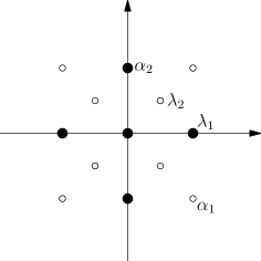
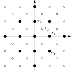
(a) $\lambda=\lambda_{1}$		(b) $\lambda=2\lambda_{1}$

Figure 3: Weight diagrams with the highest weight $\lambda=\lambda_{1}$ and $\lambda=2\lambda_{1}$. (Circles are not weights. Only the dots in black are weights.)

One should pay attention that circles in the figures are not weights. Then, the $\mathfrak{L}$-module $V(\lambda)$ can be decomposed into the direct sum of weight spaces:

$$V(\lambda)=\bigoplus_{\mu\in\Pi(\lambda)}V(\lambda)_{\mu}\,.$$ (101)

In fact, from the knowledge of weight diagrams [8], we can label the weights of $V(\lambda)$, where $\lambda=N\,\lambda_{1}$, one by one as follows: $\mu\in\Pi(\lambda)$ if and only if

$$\mu=\lambda-l\,\alpha_{1}-j\,(\alpha_{1}+\alpha_{2})\,,\qquad(0\leqslant l\leqslant N\,,\quad 0\leqslant j\leqslant 2N-2l)$$ (102)

or

$$\mu=\lambda-k\,(\alpha_{1}+2\,\alpha_{2})-j\,(\alpha_{1}+\alpha_{2})\,,\qquad(0<k\leqslant N\,,\quad 0\leqslant j\leqslant 2N-2k)\,.$$ (103)

In order for $\phi_{\lambda}^{(jkl)}$ to be nonzero, both $\phi_{\lambda}^{(00l)}$ and $\phi_{\lambda}^{(0kl)}$ must be nonzero. Consequently, the necessary condition for $\phi_{\lambda}^{(jkl)}$ to be nonzero is

$$0\leqslant l\leqslant N\,,\quad 0\leqslant k\leqslant N\,,\quad 0\leqslant j\leqslant 2\min(N-k,N-l)\,.$$ (104)

These conditions can also be obtained by analyzing the non-vanishing condition for $\phi_{\lambda}^{(jkl)}$ in eq. (81).

Notice that $\lambda_{1}=\alpha_{1}+\alpha_{2}$ and $\alpha_{2}$ are orthogonal, having the same length. So it is often convenient to write $\mu$ in eq. (99) as

$$\mu=\Big{(}n_{1}+\frac{n_{2}}{2}\Big{)}\,\lambda_{1}+\frac{n_{2}}{2}\,\alpha_{2}\,.$$ (105)

Note that $n_{2}$ is an even integer. (See, eqs. (100).) Then the necessary and sufficient condition for $\mu$ to be a weight is

$$-N\leqslant\Big{(}n_{1}+\frac{n_{2}}{2}\Big{)}+\frac{n_{2}}{2}\leqslant N\,,\qquad-N\leqslant\Big{(}n_{1}+\frac{n_{2}}{2}\Big{)}-\frac{n_{2}}{2}\leqslant N\,.$$

That is, the integer $n_{1}$ and the even integer $n_{2}$ must satisfy the following inequalities:

$$-N\leqslant n_{1}\leqslant N\,,\qquad-N\leqslant n_{1}+n_{2}\leqslant N\,.$$ (106)

This can be directly seen from the figure of $\Pi(\lambda)$, and can be derived from the label (102) and (103).

5.5 Multiplicity of Weights

One of the consequence of eq. (101) is

$$\dim V(\lambda)=\sum_{\mu\in\Pi(\lambda)}\dim V(\lambda)_{\mu}\,.$$ (107)

Traditionally $\dim V(\lambda)_{\mu}$ is called the multiplicity of $\mu$ with respect to the highest weight $\lambda$, and denoted by $m_{\lambda}(\mu)$. In Appendix C we shall prove that, for a weight $\mu=n_{1}\,\lambda_{1}+n_{2}\,\lambda_{2}$,

$$m_{\lambda}(n_{1}\,\lambda_{1}+n_{2}\,\lambda_{2})=\Big{\lfloor}\frac{N-|n_{1}+\frac{n_{2}}{2}|-|\frac{n_{2}}{2}|}{2}\Big{\rfloor}+1\,,$$ (108)

where $\lfloor\cdot\rfloor$ denotes the floor of a number. Equivalently, for a weight $l_{1}\,\lambda_{1}+l_{2}\,\alpha_{2}$, we have

$$m_{\lambda}(l_{1}\,\lambda_{1}+l_{2}\,\alpha_{2})=\Big{\lfloor}\frac{N-|l_{1}|-|l_{2}|}{2}\Big{\rfloor}+1\,.$$ (109)

See, eq. (105).

5.6 Linear Dependence

Given a weight $\mu=n_{1}\,\lambda_{1}+n_{2}\,\lambda_{2}$, the weight space $V(\lambda)_{\mu}$ is spanned by the functions $\phi_{\lambda}^{(jkl)}$ with nonnegative integers $j$, $k$ and $l$ satisfying eq. (99), or equivalently, eqs. (100). Then, arises a question: are all the nonzero functions $\phi^{(jkl)}_{\lambda}$ linearly independent?

The answer is negative. For example, when $N=1$, nonzero functions $\phi^{(jkl)}_{\lambda}$ are listed as follows.

$$\phi^{(000)}_{\lambda_{1}} =\cosh\chi\cos\zeta\,e^{-i\theta}\,,$$ (110)

$$\phi^{(001)}_{\lambda_{1}} =-\cosh\chi\sin\zeta\,e^{-i\varphi}\,,$$ (111)

$$\phi^{(010)}_{\lambda_{1}} =\cosh\chi\sin\zeta\,e^{i\varphi}\,,$$ (112)

$$\phi^{(011)}_{\lambda_{1}} =\cosh\chi\cos\zeta\,e^{i\theta}\,,$$ (113)

$$\phi^{(100)}_{\lambda_{1}} =-2\sinh\chi\,,$$ (114)

$$\phi^{(200)}_{\lambda_{1}} =2\cosh\chi\cos\zeta\,e^{i\theta}\,.$$ (115)

Obviously, $\phi^{(011)}_{\lambda_{1}}$ and $\phi^{(200)}_{\lambda_{1}}$ are linearly dependent.

5.7 Nonexistence of Infinite Dimensional $\mathfrak{L}$-Submodules in $C^{\infty}(dS^{4})$

So far the Verma modules contained in $C^{\infty}(dS^{4})$ are all irreducible and finite dimensional. There is a question, then, whether there exist any infinite dimensional irreducible $\mathfrak{L}$-submodules of $C^{\infty}(dS^{4})$, where $\mathfrak{L}=\mathfrak{so}(1,4)\otimes_{\mathbb{R}}\mathbb{C}$. The answer is negative.

In §5.2, the Verma modules are constructed according to the representation theory[8] of semisimple Lie algebras: We first start from a dominant weight $\lambda$ as the highest weight. Then, in the process of determining the maximal vector $\phi_{\lambda}$, the highest weight is also determined to be $N\lambda_{1}$, with $N$ a nonnegative integer.

In §5.2, the reason for $N$ to be a nonnegative integer comes from the representation theory of semisimple Lie algebras: an irreducible highest weight module is finite dimensional if and only if its highest weight is dominant and integral [8].

In fact, in §5.2 we need not refer to the representation theory, just remaining $N$ in eq. (80) to be an unknown parameter. Now that the maximal vector $\phi_{\lambda}$ has been determined in the form of eq. (80), the parameter $N$ must be an integer because of the periodicity of $\theta$. See, eqs. (61) and (62). If $N$ is negative, however, the function $\widetilde{\phi}_{\lambda}$ in eq. (94) is not a smooth function on $\mathbb{R}^{1,4}-\{\mathbf{0}\}$. Since the pullback (or, naively, restriction) of $\widetilde{\phi}_{\lambda}$ to $U\subset dS^{4}$ is just $\phi_{\lambda}$, the latter cannot be extended to be a smooth function on $dS^{4}$ provided $N<0$. Hence, without referring to the representation theory of semisimple Lie algebras, we can still determine that $N$ is a nonnegative integer. Hence, a Verma module $V(N\lambda_{1})$ is always finite dimensional and irreducible.

In one word, an irreducible $\mathfrak{L}$-submodule of $C^{\infty}(dS^{4})$ is always finite dimensional, being a Verma module $V(N\lambda_{1})$ with $N$ a nonnegative integer.

6 Smooth Solutions and Masses of the Klein-Gordon Scalars on $dS^{4}$

6.1 Imaginary and Discrete Masses of the Klein-Gordon Equation on $dS^{4}$

It is well known that

$$C=\frac{1}{2}\,\eta^{AC}\eta^{BD}\,X_{AB}X_{CD}$$ (116)

is a universal Casimir element of $\mathfrak{L}=\mathfrak{so}(1,4)\otimes_{\mathbb{R}}\mathbb{C}$. When acting on the irreducible $\mathfrak{L}$-module $V(\lambda)$, where $\lambda=N\lambda_{1}$, $X_{AB}$ is replaced by the Lie derivative $L_{\mathbf{X}_{AB}}$, or directly, the vector field $\mathbf{X}_{AB}$. So is $h_{\alpha_{1}}$, $e_{\alpha_{1}}$, $f_{\alpha_{1}}$, and so on, in the following. Using the expressions (39) to (43), we can verify that

$$C =-\frac{1}{2}\,h_{\alpha_{1}}(2h_{\alpha_{1}}+h_{\alpha_{2}})-\frac{1}{2}\,h_{\alpha_{2}}(h_{\alpha_{1}}+h_{\alpha_{2}})-(e_{\alpha_{1}}f_{\alpha_{1}}+f_{\alpha_{1}}e_{\alpha_{1}})-\frac{1}{2}\,(e_{\alpha_{2}}f_{\alpha_{2}}+f_{\alpha_{2}}e_{\alpha_{2}})$$

$$-\frac{1}{2}\,(e_{\alpha_{1}+\alpha_{2}}f_{\alpha_{1}+\alpha_{2}}+f_{\alpha_{1}+\alpha_{2}}e_{\alpha_{1}+\alpha_{2}})-(e_{\alpha_{1}+2\alpha_{2}}f_{\alpha_{1}+2\alpha_{2}}+f_{\alpha_{1}+2\alpha_{2}}e_{\alpha_{1}+2\alpha_{2}})\,.$$ (117)

First using the commutators in Appendix A, then using eqs. (126), we can reduce the above expression to

$$C =-h_{\alpha_{1}}h_{\alpha_{1}}-h_{\alpha_{1}}h_{\alpha_{2}}-\frac{1}{2}\,h_{\alpha_{2}}h_{\alpha_{2}}-3\,h_{\alpha_{1}}-2\,h_{\alpha_{2}}$$

$$\phantom{={}}-2\,f_{\alpha_{1}}e_{\alpha_{1}}-f_{\alpha_{2}}e_{\alpha_{2}}-f_{\alpha_{1}+\alpha_{2}}e_{\alpha_{1}+\alpha_{2}}-2\,f_{\alpha_{1}+2\alpha_{2}}e_{\alpha_{1}+2\alpha_{2}}\,.$$ (118)

When $C$ acts on $\phi_{\lambda}$, there is simply

$$C.\phi_{\lambda} =-h_{\alpha_{1}}h_{\alpha_{1}}.\phi_{\lambda}-h_{\alpha_{1}}h_{\alpha_{2}}.\phi_{\lambda}-\frac{1}{2}\,h_{\alpha_{2}}h_{\alpha_{2}}.\phi_{\lambda}-3\,h_{\alpha_{1}}.\phi_{\lambda}-2\,h_{\alpha_{2}}.\phi_{\lambda}$$

$$=-[\lambda(h_{\alpha_{1}})]^{2}\phi_{\lambda}-\lambda(h_{\alpha_{2}})\,\lambda(h_{\alpha_{1}})\,\phi_{\lambda}-\frac{1}{2}\,[\lambda(h_{\alpha_{2}})]^{2}\phi_{\lambda}-3\,\lambda(h_{\alpha_{1}})\,\phi_{\lambda}-2\,\lambda(h_{\alpha_{2}})\,\phi_{\lambda}\,.$$

Note that $\lambda(h_{\alpha_{1}})=N\,\lambda_{1}(h_{\alpha_{1}})=N$ and $\lambda(h_{\alpha_{2}})=N\,\lambda_{1}(h_{\alpha_{2}})=0$. Hence

$$C.\phi_{\lambda} =-N^{2}\,\phi_{\lambda}-3N\,\phi_{\lambda}=-N\,(N+3)\,\phi_{\lambda}\,.$$

Since $V(\lambda)$ is an irreducible $\mathfrak{L}$-module, according to Schur’s lemma, every $\phi\in V(\lambda)$ satisfies

$$C.\phi=-N\,(N+3)\,\phi\,.$$ (119)

Comparing it with eq. (19), we have the mass $m$ of the Klein-Gordon field $\phi$, as shown in the following:

$$m^{2}=-\frac{N(N+3)\,\hbar^{2}}{c^{2}l^{2}}\,.$$ (120)

It is significant that the mass is not only discrete, but also an imaginary quantity. In the classical level, this doesn’t matter, because $m$ only makes sense in the quantum level. The detailed consequence and discussion of this fact in QFT will be presented in other papers.

6.2 Irreducibility of the Solution Space of a Klein-Gordon Equation

So far we have shown that the Klein-Gordon equation on $dS^{4}$ must be of the form

$$g^{ab}\,\nabla_{a}\nabla_{b}\phi-\frac{N\,(N+3)}{l^{2}}\,\phi=0$$ (121)

with certain a nonnegative integer $N$. We have shown that each smooth function $\phi\in V(N\lambda_{1})$ is a solution of the above equation. That is, the irreducible $\mathfrak{L}$-module $V(N\lambda_{1})$ is a linear subspace of the solution space $\mathscr{S}_{\textrm{KG}}(dS^{4})$ of eq. (121). Since $\mathscr{S}_{\textrm{KG}}(dS^{4})$ is also an $\mathfrak{L}$-module, but not necessarily irreducible, it must be the direct sum of $V(N^{\prime}\lambda_{1})$ with $N^{\prime}\geqslant 0$ satisfying

$$N^{\prime}\,(N^{\prime}+3)=N\,(N+3)\,.$$

It is easy to check that the only possibility is $N^{\prime}=N$. Consequently, the solution space of eq. (121) is $V(N\lambda_{1})$, the irreducible $\mathfrak{L}$-module having $N\lambda_{1}$ as its highest weight.

So, a general smooth solution of the Klein-Gordon equation on $dS^{4}$, namely, eq. (121), is

$$\phi=\sum_{l=0}^{N}\sum_{k=0}^{N}\sum_{j=0}^{2N-2\max(k,l)}a_{jkl}\,\phi^{(jkl)}_{N\lambda_{1}}\,,$$ (122)

where $a_{jkl}$ are some complex constants. Although the functions $\phi^{(jkl)}_{N\lambda_{1}}$ are possibly linearly dependent, the conclusion remains true, only that the coefficients $a_{jkl}$ for a given solution are not uniquely determined.

7 Conclusions and Discussion

There are papers, such as [14] and [15], discussing the solutions of the Klein-Gordon equation on $dS^{4}$. The discussion in [14] does not evaluate the effects influenced by the global structures of the spacetime. Note that the elegant method in [10] can be applied to $dS^{4}$, too. But the solutions obtained in [10] are massless scalars, and the smoothness of these solutions were not discussed. By imposing the condition of quadratically integrable on the whole $dS^{4}$, it is shown in [15] that the mass $m$ of Klein-Gordon fields on $dS^{4}$ satisfies (in the natural units)

$$m^{2}=\lambda_{jn}=\frac{9}{4}-\Big{(}j+\frac{1}{2}-n\Big{)}^{2}$$

with $j$, $n=0$, 1, 2, …such that $j+\frac{1}{2}-n>0$. If we set $N=j-n-1$, there will be $N>-\frac{3}{2}$ and $m^{2}=-N(N+3)$. In Theorem 2 in [15] it is stated that $m^{2}$ could be positive (then equal to 2), and that the solution space for each $\lambda_{jn}$ is infinite dimensional. Although the mass spectrum is very similar to ours, but in some details, the conclusions are quite different. Since there is no detailed proof in [15], this will be left as an open question.

By using the Lie group and Lie algebra method, we have obtained all smooth solutions of a Klein-Gordon equation in the de Sitter background, forming a finite dimensional irreducible $\mathfrak{L}$-module, with $\mathfrak{L}=\mathfrak{so}(1,4)\otimes_{\mathbb{R}}\mathbb{C}$. An associated conclusion is that the mass of a Klein-Gordon equation on $dS^{4}$ cannot be arbitrary. It’s square must be non-positive and discrete, as shown in eq. (120).

In this paper we construct the irreducible $\mathfrak{L}$-modules with respect to the Cartan subalgebra $\mathfrak{h}^{\prime}$, spanned by $X_{12}$ and $X_{34}$. Coordinate systems and weight spaces can be constructed with respect to the Cartan subalgebra $\mathfrak{h}$, spanned by $X_{12}$ and $X_{04}$. Detailed discussion will be presented in other papers.

So far, it is not so factory that the functions $\phi^{(jkl)}_{N\lambda_{1}}$ (with $j$, $k$ and $l$ satisfying the condition (104)) might be not linearly independent. But the details of a solution is not our main topic in this paper. These are left for future papers. As a consequence, it is not quite suitable for now to discuss the quantization of Klein-Gordon fields in the de Sitter background.

But problem due to the mass must be discussed here. When viewed as a relativistic quantum mechanical equation, the Klein-Gordon equation in the Minkowski background is obtained by applying the quantization rule

$$p_{\mu}\to\hat{p}_{\mu}=i\hbar\frac{\partial}{\partial x^{\mu}}$$

to the relation $\eta_{\mu\nu}\,p^{\mu}p^{\nu}=m^{2}c^{2}$. Then, from the Klein-Gordon equation in the Minkowski background to that in a curved spacetime, we need only to replace the partial derivative to the covariant derivative. Unfortunately, in the case of de Sitter background, we have seen that the mass is no longer real (except when $N=0$).

What if we exchange these two steps: first establishing the classical mechanics in the de Sitter background, then quantizing it? H.-Y. Guo et al have attempted the first step: trying their best to establish a classical mechanics resembling the relativistic mechanics. For a free particle in $dS^{4}$, there exists a conserved 5-angular momentum $\mathcal{L}_{AB}$, satisfying the equality

$$-\frac{1}{2l^{2}}\,\eta^{AC}\eta^{BD}\,\mathcal{L}_{AB}\mathcal{L}_{CD}=\frac{E^{2}}{c^{2}}-\boldsymbol{P}^{2}-\frac{1}{2l^{2}}\,\boldsymbol{L}^{2}=m_{\Lambda 0}^{2}c^{2}\,,$$ (123)

where $E$, $\boldsymbol{P}$ and $\boldsymbol{L}$ are the splitting of the 5-angular momentum with respect to a Beltrami coordinate system, and $m_{\Lambda 0}$ is the proper mass of the particle [16, 17, 18, 19]. When $l\to\infty$, $(E/c,\boldsymbol{P})$ tends to the 4-momentum in Einstein’s special relativity, while $\boldsymbol{L}/l\to 0$. Under a reasonable quantization rule

$$\mathcal{L}_{AB}\rightarrow i\hbar\,\mathbf{X}_{AB}\,,$$ (124)

the above equation will yield a “quantum” equation

$$\frac{\hbar^{2}}{2l^{2}}\,\eta^{AC}\eta^{BD}\,L_{\mathbf{X}_{AB}}L_{\mathbf{X}_{CD}}\phi=m_{\Lambda 0}^{2}c^{2}\,\phi\,,$$

namely, the Klein-Gordon equation (2). Unfortunately still, in the classical level, i.e., in eq. (123), the mass $m_{\Lambda 0}$ is nonnegative, while in the resulted “quantum” equation, $m_{\Lambda 0}^{2}\leqslant 0$.

This really sounds bad, because the process of quantization and the process of generalizing to curved spacetime seems not so compatible. For long there are some physicists believing that general relativity and quantum theory are not compatible. Even if they were wrong eventually, this problem is at least very serious and hard currently: before we settled down to investigation of QFT in the de Sitter background, we must suitably solve the problem of $m^{2}\leqslant 0$.

Another belief is, when the cosmological radius $l\to\infty$ in $dS^{4}$, physical laws and phenomena tend to those in the Minkowski spacetime. The Klein-Gordon equation is again an exception: On the one hand, the problem of $m^{2}\leqslant 0$ is still the obstacle. On the other hand, the dimension of the solution space is also an obstacle, with the one for the Minkowski space being infinite dimensional, while the one for $dS^{4}$ being finite dimensional.

At last, we point out that the method in this paper can be applied to various field equations in de Sitter spacetime or anti-de Sitter spacetime. These will be presented in other papers. For other spacetimes with sufficient symmetries, this method might be effective, too.

Appendix A The Commutators of $\mathfrak{so}(1,4)\otimes_{\mathbb{R}}\mathbb{C}$

The formulae in this section are satisfied, no matter the Cartan subalgebra is $\mathfrak{h}$ in §4.3 or $\mathfrak{h}^{\prime}$ in §4.4.

First of all, for each $\alpha$ and $\beta\in\Phi^{+}$, there are the standard commutators

$$[h_{\alpha},e_{\beta}]=\beta(h_{\alpha})\,e_{\beta}\,,\qquad[h_{\alpha},f_{\beta}]=-\beta(h_{\alpha})\,f_{\beta}\,,\qquad[e_{\beta},f_{\beta}]=h_{\beta}\,.$$ (125)

Note that

$$h_{\alpha_{1}+\alpha_{2}}=2\,h_{\alpha_{1}}+h_{\alpha_{2}}\,,\qquad h_{\alpha_{1}+2\alpha_{2}}=h_{\alpha_{1}}+h_{\alpha_{2}}\,.$$ (126)

Thus, $\beta(h_{\alpha})$ for all $\alpha$ and $\beta\in\Phi^{+}$ can be obtained by virtue of the linear property of $\beta$ and the Cartan integers

$$\alpha_{i}(h_{\alpha_{j}})=\langle\alpha_{i},\alpha_{j}\rangle$$ (127)

for $i$, $j=1$ and $2$.

Next, the following commutators are satisfied by the Chevalley bases in both §4.3 and §4.4:

$$[e_{\alpha_{1}},e_{\alpha_{2}}] =e_{\alpha_{1}+\alpha_{2}}\,, [e_{\alpha_{1}},e_{\alpha_{1}+\alpha_{2}}] =0\,, [e_{\alpha_{1}},e_{\alpha_{1}+2\alpha_{2}}] =0\,,$$ (128)

$$[e_{\alpha_{2}},e_{\alpha_{1}+\alpha_{2}}] =2\,e_{\alpha_{1}+2\alpha_{2}}\,, [e_{\alpha_{2}},e_{\alpha_{1}+2\alpha_{2}}] =0\,, [e_{\alpha_{1}+\alpha_{2}},e_{\alpha_{1}+2\alpha_{2}}] =0\,,$$ (129)

$$[f_{\alpha_{1}},f_{\alpha_{2}}] =-f_{\alpha_{1}+\alpha_{2}}\,, [f_{\alpha_{1}},f_{\alpha_{1}+\alpha_{2}}] =0\,, [f_{\alpha_{1}},f_{\alpha_{1}+2\alpha_{2}}] =0\,,$$ (130)

$$[f_{\alpha_{2}},f_{\alpha_{1}+\alpha_{2}}] =-2\,f_{\alpha_{1}+2\alpha_{2}}\,,\qquad [f_{\alpha_{2}},f_{\alpha_{1}+2\alpha_{2}}] =0\,,\qquad [f_{\alpha_{1}+\alpha_{2}},f_{\alpha_{1}+2\alpha_{2}}] =0\,,$$ (131)

$$[e_{\alpha_{1}},f_{\alpha_{2}}] =0\,, [e_{\alpha_{1}},f_{\alpha_{1}+\alpha_{2}}] =-f_{\alpha_{2}}\,, [e_{\alpha_{1}},f_{\alpha_{1}+2\alpha_{2}}] =0\,,$$ (132)

$$[e_{\alpha_{2}},f_{\alpha_{1}}] =0\,, [e_{\alpha_{2}},f_{\alpha_{1}+\alpha_{2}}] =2f_{\alpha_{1}}\,, [e_{\alpha_{2}},f_{\alpha_{1}+2\alpha_{2}}] =-f_{\alpha_{1}+\alpha_{2}}\,,$$ (133)

$$[e_{\alpha_{1}+\alpha_{2}},f_{\alpha_{1}}] =-e_{\alpha_{2}}\,, [e_{\alpha_{1}+\alpha_{2}},f_{\alpha_{2}}] =2\,e_{\alpha_{1}}\,, [e_{\alpha_{1}+\alpha_{2}},f_{\alpha_{1}+2\alpha_{2}}] =f_{\alpha_{2}}\,,$$ (134)

$$[e_{\alpha_{1}+2\alpha_{2}},f_{\alpha_{1}}] =0\,, [e_{\alpha_{1}+2\alpha_{2}},f_{\alpha_{2}}] =-e_{\alpha_{1}+\alpha_{2}}\,,\quad [e_{\alpha_{1}+2\alpha_{2}},f_{\alpha_{1}+\alpha_{2}}] =e_{\alpha_{2}}\,.$$ (135)

Appendix B Irreducibility of the Verma Module $V(\lambda)$

According to the representation theory of Lie algebras, the function in eq. (81) belongs to the weight

$$\mu =\lambda-j\,(\alpha_{1}+\alpha_{2})-k\,(\alpha_{1}+2\alpha_{2})-l\,\alpha_{1}=N\,\lambda_{1}-(j+k+l)\,\alpha_{1}-(j+2k)\,\alpha_{2}$$

$$=n_{1}\,\lambda_{1}+n_{2}\,\lambda_{2}\,,$$ (136)

where

$$n_{1}=N-j-2l\,,\qquad n_{2}=-2\,(k-l)\,.$$ (137)

That is, it satisfies the conditions

$$h_{\alpha_{1}}.\phi_{\lambda}^{(jkl)} =L_{\mathbf{h}_{\alpha_{1}}}\phi_{\lambda}^{(jkl)}=\mu(h_{\alpha_{1}})\,\phi_{\lambda}^{(jkl)}=n_{1}\,\phi_{\lambda}^{(jkl)}\,,$$ (138)

$$h_{\alpha_{2}}.\phi_{\lambda}^{(jkl)} =L_{\mathbf{h}_{\alpha_{2}}}\phi_{\lambda}^{(jkl)}=\mu(h_{\alpha_{2}})\,\phi_{\lambda}^{(jkl)}=n_{2}\,\phi_{\lambda}^{(jkl)}\,,$$ (139)

which can be obviously seen from eqs. (81), (65) and (66).

In order that $\phi_{\lambda}^{(jkl)}\neq 0$ in $V(\lambda)$ (meaning that this function is nonzero somewhere on $dS^{4}$), there must be $j+k+l\leqslant N$, namely,

$$n_{1}+\frac{n_{2}}{2}\geqslant 0\,.$$ (140)

If $V(\lambda)$ is reducible, there exists at least one nontrivial Verma submodule $V(\lambda^{\prime})$ in $V(\lambda)$, where $\lambda^{\prime}=N^{\prime}\lambda_{1}$ with $N^{\prime}<N$. Equivalently, there are some constants $a_{jkl}\in\mathbb{C}$, which are not all zero, satisfying

$$\sum_{j\geqslant 0}\sum_{k\geqslant 0}\sum_{l\geqslant 0}a_{jkl}\,\phi_{\lambda}^{(jkl)}=(\cosh\chi\cos\zeta\,e^{-i\theta})^{N^{\prime}}\,,$$

with $0\leqslant N^{\prime}<N$. By virtue of the expression (81), we have the first observation that $a_{jkl}=0$ whenever $k\neq l$. Now that $a_{jll}$ is abbreviated as $a_{j,l}$, we have the second observation that $a_{j,l}=0$ whenever $j\neq N-N^{\prime}-2l$. In the following $a_{N-N^{\prime}-2l,l}$ is abbreviated as $a_{l}$. Then the above condition turns out to be

$$\sum_{l=0}^{\lfloor\frac{N-N^{\prime}}{2}\rfloor}a_{l}\,\phi_{\lambda}^{(N-N^{\prime}-2l,\,l,\,l)}=(\cosh\chi\cos\zeta\,e^{-i\theta})^{N^{\prime}}\,,$$

namely,

$$\sum_{l=0}^{\lfloor\frac{N-N^{\prime}}{2}\rfloor}\sum_{j^{\prime}=0}^{\lfloor\frac{N-N^{\prime}}{2}\rfloor-l}\sum_{k^{\prime}=0}^{l}(-1)^{N-N^{\prime}-l+k^{\prime}}2^{N-N^{\prime}-2l-2j^{\prime}}\,a_{l}$$

$$\qquad\frac{N!}{(N^{\prime}+j^{\prime}+k^{\prime})!}\,\frac{l!}{(l-k^{\prime})!}\,\frac{l!}{k^{\prime}!\,(l-k^{\prime})!}\,\frac{(N-N^{\prime}-2l)!}{j^{\prime}!\,(N-N^{\prime}-2l-2j^{\prime})!}$$

$$\qquad(\cosh^{N^{\prime}+2l+2j^{\prime}}\chi)(\sinh^{N-N^{\prime}-2l-2j^{\prime}}\chi)(\cos^{N^{\prime}+2j^{\prime}+2k^{\prime}}\zeta)(1-\cos^{2}\zeta)^{l-k^{\prime}}\,e^{-i\,N^{\prime}\,\theta}$$

$$= (\cosh\chi\cos\zeta\,e^{-i\theta})^{N^{\prime}}\,.$$

Observation of the exponent of $\sinh\chi$ indicates that $N-N^{\prime}$ must be an even integer. Set $N-N^{\prime}=2n$. Then the above condition becomes

$$\sum_{l=0}^{n}\sum_{j^{\prime}=0}^{n-l}\sum_{k^{\prime}=0}^{l}(-1)^{l+k^{\prime}}4^{n-l-j^{\prime}}\,a_{l}\,b(N,n,j^{\prime},k^{\prime},l)\,(\cosh^{2}\chi)^{l+j^{\prime}}(\cosh^{2}\chi-1)^{n-l-j^{\prime}}(\cos^{2}\zeta)^{j^{\prime}+k^{\prime}}(1-\cos^{2}\zeta)^{l-k^{\prime}}=1\,,$$

or, equivalently,

$$\sum_{j^{\prime}=0}^{n}\sum_{k^{\prime}=0}^{n-j^{\prime}}\sum_{l=k^{\prime}}^{n-j^{\prime}}(-1)^{l+k^{\prime}}4^{n-l-j^{\prime}}\,a_{l}\,b(N,n,j^{\prime},k^{\prime},l)\,(\cosh^{2}\chi)^{l+j^{\prime}}(\cosh^{2}\chi-1)^{n-l-j^{\prime}}(\cos^{2}\zeta)^{j^{\prime}+k^{\prime}}(1-\cos^{2}\zeta)^{l-k^{\prime}}=1\,,$$ (141)

where

$$b(N,n,j^{\prime},k^{\prime},l)=\frac{N!}{(N-2n+j^{\prime}+k^{\prime})!}\frac{l!}{(l-k^{\prime})!}\frac{l!}{k^{\prime}!\,(l-k^{\prime})!}\frac{(2n-2l)!}{j^{\prime}!\,(2n-2l-2j^{\prime})!}\,.$$

We can see from eq. (141) that, for the existence of $a_{l}$’s that are not all zero, there must be $n=0$, namely, $N^{\prime}=N$. However, when $N^{\prime}=N$, the Verma submodule $V(\lambda^{\prime})=V(\lambda)$ is no longer trivial. This proves the irreducibility of the Verma module $V(\lambda)$.

Appendix C Proof of Eq. (108)

In this appendix we prove the formula (108).

Each root $\alpha$ can be associated with a linear transformation $\sigma_{\alpha}$ on $\mathfrak{h}^{\prime*}$, called a Weyl reflection, sending $\mu\in\mathfrak{h}^{\prime*}$ to $\sigma_{\alpha}(\mu)\in\mathfrak{h}^{\prime*}$, where

$$\sigma_{\alpha}(\mu):=\mu-\frac{2\,(\mu,\alpha)}{(\alpha,\alpha)}\,\alpha=\mu-\langle\mu,\alpha\rangle\,\alpha\,.$$ (142)

A weight $\mu=n_{1}\,\lambda_{1}+n_{2}\,\lambda_{2}$ with $n_{1}\geqslant 0$ and $n_{2}\geqslant 0$ is called dominant. Then any weight $\mu\in\Pi(\lambda)$ can be obtained from a dominant weight via a series of Weyl reflections [8]: there exist a dominant weight $\mu^{\prime}$ and some roots $\beta_{1}$, …, $\beta_{n}$ so that $\mu=\sigma_{\beta_{n}}\cdots\sigma_{\beta_{1}}(\mu^{\prime})$. Another important fact [8] is that, for any $\mu\in\mathfrak{h}^{\prime*}$ and any root $\alpha$,

$$m_{\lambda}(\sigma_{\alpha}(\mu))=m_{\lambda}(\mu)\,.$$ (143)

It is easy to verify that eq. (108) does satisfy the above condition. The consequence of the above facts is, in order to prove the formula (108) for arbitrary weight, it is sufficient to prove it for each dominant weights.

Note that, when $n_{1}\,\lambda_{1}+n_{2}\,\lambda_{2}$ is a dominant weight, eq. (108) turns out to be

$$m_{\lambda}(n_{1}\,\lambda+n_{2}\,\lambda_{2})=\Big{\lfloor}\frac{N-n_{1}-n_{2}}{2}\Big{\rfloor}+1\,.$$ (144)

We are going to use the Freudenthal formula [8]

$$[(\lambda+\delta,\lambda+\delta)-(\mu+\delta,\mu+\delta)]m_{\lambda}(\mu)=2\sum_{\alpha\in\Phi^{+}}\sum_{i=1}^{\infty}(\mu+i\,\alpha,\alpha)\,m_{\lambda}(\mu+i\,\alpha)$$ (145)

to prove eq. (144) recursively, where

$$\delta=\frac{1}{2}\sum_{\beta\in\Phi^{+}}\beta=2\,(\alpha_{1}+\alpha_{2})-\frac{1}{2}\,\alpha_{1}\,.$$ (146)

Note that a weight $\mu=n_{1}\,\lambda_{1}+n_{2}\,\lambda_{2}$ can be expressed as $\mu=\lambda-L\,(\alpha_{1}+\alpha_{2})-l\,\alpha_{1}$, where

$$L:=N-n_{1}-n_{2}\,,\qquad l:=\frac{n_{2}}{2}\,.$$

Then, the recursion is based on $L$ and $l$.

The necessary and sufficient condition for $\mu=\lambda-L\,(\alpha_{1}+\alpha_{2})-l\,\alpha_{1}$ to be dominant is: $L$ and $l$ are integers satisfying

$$0\leqslant L\leqslant N\,,\qquad 0\leqslant l\leqslant\Big{\lfloor}\frac{L}{2}\Big{\rfloor}\,.$$

Furthermore, by virtue of

$$\lambda-\mu =L\,(\alpha_{1}+\alpha_{2})+l\,\alpha_{1}\,,$$ (147)

$$\mu+\delta =(N-L+2)\,(\alpha_{1}+\alpha_{2})-\Big{(}l+\frac{1}{2}\Big{)}\,\alpha_{1}$$ (148)

and the data of inner product in eq. (29), we have

$$(\lambda+\delta,\lambda+\delta)-(\mu+\delta,\mu+\delta) =(\lambda-\mu,\lambda-\mu)+2\,(\lambda-\mu,\mu+\delta)$$

$$=\frac{L}{6}\,(2N-L+3)+\frac{l}{3}\,(N-L-l+1)\,.$$ (149)

The Verma module $V(\lambda)$ is generated out of the highest weight $\lambda$. Hence $m_{\lambda}(\lambda)=1$. If $N=0$, the only weight is $\lambda=0$ itself; If $N=1$, the only dominant is $\lambda=\lambda_{1}$ itself. In these cases eq. (144) is obviously correct. In the following proof we assume that $N\geqslant 2$.

We first recursively prove that a dominant weight $\mu=\lambda-l\,\alpha_{1}$ has $m_{\lambda}(\mu)=1$. In fact, when $l=0$, one has $\mu=\lambda$, for which $m_{\lambda}(\mu)=1$ is obviously correct. As a recursion assumption, we assume that $l>0$ and that $m_{\lambda}(\lambda-i\,\alpha_{1})=1$ for all $i$ satisfying $0\leqslant i\leqslant l-1$. The Freudenthal formula for $\mu=\lambda-l\,\alpha_{1}$, then, turns out to be

$$\frac{l}{3}\,(N-l+1)\,m_{\lambda}(\mu) =2\sum_{\alpha\in\Phi^{+}}\sum_{i=1}^{\infty}(\mu+i\,\alpha,\alpha)\,m_{\lambda}(\mu+i\,\alpha)\,.$$

For a positive root $\alpha$ and a positive integer $i$, $\mu+i\,\alpha=\lambda-l\,\alpha_{1}+i\,\alpha$ is a weight (hence $m_{\lambda}(\mu+i\,\alpha)\neq 0$) if and only if $\alpha=\alpha_{1}$, together with $1\leqslant i\leqslant l$. Thus the above equation results in

$$\frac{l}{3}\,(N-l+1)\,m_{\lambda}(\mu) =2\sum_{i=1}^{l}(\mu+i\,\alpha_{1},\alpha_{1})\,m_{\lambda}(\mu+i\,\alpha_{1})$$

$$=2\sum_{i=1}^{l}(\lambda-(l-i)\,\alpha_{1},\alpha_{1})\,m_{\lambda}(\lambda-(l-i)\,\alpha_{1})$$

$$=2\sum_{i=0}^{l-1}(\lambda-i\,\alpha_{1},\alpha_{1})\,m_{\lambda}(\lambda-i\,\alpha_{1})$$

$$=2\sum_{i=0}^{l-1}(\lambda-i\,\alpha_{1},\alpha_{1})\,.$$

In the last step we have used the recursion assumption $m_{\lambda}(\lambda-i\,\alpha_{1})=1$ for $0\leqslant i\leqslant l-1$. The right hand side of the above is

$$2\sum_{i=0}^{l-1}\Big{(}\frac{N}{6}-\frac{i}{3}\Big{)}=\frac{l}{3}\,(N-l+1)\,.$$

Hence we have $m_{\lambda}(\mu)=m_{\lambda}(\lambda-l\alpha_{1})=1$. This recursively proves that eq. (144) is correct when $n_{1}+n_{2}=N$.

Next, for an arbitrary weight $\mu=n_{1}\,\lambda_{1}+n_{2}\,\lambda_{2}$, we can observe eq. (105) and prove that $N-|n_{1}+\frac{n_{2}}{2}|-|\frac{n_{2}}{2}|$ is an invariant under the action of the Weyl group (which is generated by the Weyl reflections). The meaning of this statement is, if $w(\mu)=n^{\prime}_{1}\,\lambda_{1}+n^{\prime}_{2}\,\lambda_{2}$ where $w$ is the composition of some Weyl reflections, there will always be the equality

$$N-\Big{|}n^{\prime}_{1}+\frac{n^{\prime}_{2}}{2}\Big{|}-\Big{|}\frac{n^{\prime}_{2}}{2}\Big{|}=N-\Big{|}n_{1}+\frac{n_{2}}{2}\Big{|}-\Big{|}\frac{n_{2}}{2}\Big{|}\,.$$ (150)

So far, by virtue of the Weyl reflections, we have proved that eq. (108) is valid whenever $N-|n_{1}+\frac{n_{2}}{2}|-|n_{2}|=0$.

For convenience, if $\mu=n_{1}\,\lambda_{1}+n_{2}\,\lambda_{2}=l_{1}\,\lambda_{1}+l_{2}\,\alpha_{2}$ is a weight, we call the invariant $N-|n_{1}+\frac{n_{2}}{2}|-|\frac{n_{2}}{2}|=N-|l_{1}|-|l_{2}|$ the level of $\mu$.

At last, we make the recursion assumption. Let $L$ be an integer satisfying $0<L\leqslant N$. We assume that eq. (108) is valid whenever $N-|n_{1}+\frac{n_{2}}{2}|-|\frac{n_{2}}{2}|<L$. Then we want to prove that eq. (144) is true for dominant weights of level $L$. As a conseqence, eq. (144) is valid for all dominant weights, hence eq. (108) is valid for all weights.

Since such a dominant weight could be expressed as $\lambda-L\,(\alpha_{1}+\alpha_{2})-l\,\alpha_{1}$, this proof is recursive by $l$, made up by three steps.

Step 1. To prove that eq. (144) is valid for the dominant weight $\mu=\lambda-L\,(\alpha_{1}+\alpha_{2})$. For this weight, the Freudenthal formula becomes

$$\frac{L}{6}\,(2N-L+3)\,m_{\lambda}(\mu) =2\sum_{i=1}^{\infty}(\mu+i\,\alpha_{1},\alpha_{1})\,m_{\lambda}(\mu+i\,\alpha_{1})+2\sum_{i=1}^{\infty}(\mu+i\,\alpha_{2},\alpha_{2})\,m_{\lambda}(\mu+i\,\alpha_{2})$$

$$+2\sum_{i=1}^{\infty}(\mu+i\,(\alpha_{1}+\alpha_{2}),\alpha_{1}+\alpha_{2})\,m_{\lambda}(\mu+i\,(\alpha_{1}+\alpha_{2}))$$

$$+2\sum_{i=1}^{\infty}(\mu+i\,(\alpha_{1}+2\alpha_{2}),\alpha_{1}+2\alpha_{2})\,m_{\lambda}(\mu+i\,(\alpha_{1}+2\alpha_{2}))\,.$$ (151)

The summands involve the following weights:

$$\mu+i\,\alpha_{1} =(N-L+i)\,\lambda_{1}-i\,\alpha_{2}\,,\qquad (1\leqslant i\leqslant\lfloor L/2\rfloor)\,;$$

$$\mu+i\,\alpha_{2} =(N-L)\,\lambda_{1}+i\,\alpha_{2}\,, (1\leqslant i\leqslant L)\,;$$

$$\mu+i\,(\alpha_{1}+\alpha_{2}) =(N-L+i)\,\lambda_{1}\,, (1\leqslant i\leqslant L)\,;$$

$$\mu+i\,(\alpha_{1}+2\alpha_{2}) =(N-L+i)\,\lambda_{1}+i\,\alpha_{2}\,, (1\leqslant i\leqslant\lfloor L/2\rfloor)\,.$$

In fact, when $L=1$, there exists no weights like $\mu+i\,\alpha_{1}$ or $\mu+i\,(\alpha_{1}+2\alpha_{2})$, with $i$ a positive integer. So this must be specially treated. In this case $\mu=(N-1)\,\lambda_{1}$, reducing eq. (151) to

$$\frac{1}{3}\,(N+1)\,m_{\lambda}(\mu)=2\,((N-1)\,\lambda_{1}+\alpha_{2},\alpha_{2})\,m_{\lambda}((N-1)\,\lambda_{1}+\alpha_{2})+2\,(N\,\lambda_{1},\lambda_{1})\,m_{\lambda}(N\,\lambda_{1})=\frac{N+1}{3}\,.$$

Therefore, for $\mu=(N-1)\,\lambda_{1}$, we have $m_{\lambda}((N-1)\,\lambda_{1})=1$, satisfying eq. (144).

In the generic case, $1<L\leqslant N$. On account of the recursion assumption, eq. (151) is reduced to

$$\frac{L}{6}\,(2N-L+3)\,m_{\lambda}(\mu) =2\sum_{i=1}^{\lfloor L/2\rfloor}\frac{N-L+2i}{3}\,\Big{(}\Big{\lfloor}\frac{L}{2}\Big{\rfloor}-i+1\Big{)}+\sum_{i=1}^{L}\frac{N-L+2i}{3}\,\Big{(}\Big{\lfloor}\frac{L-i}{2}\Big{\rfloor}+1\Big{)}$$

$$=2\sum_{i=1}^{\lfloor L/2\rfloor}\frac{N-L+2i}{3}\,\Big{(}\Big{\lfloor}\frac{L}{2}\Big{\rfloor}-i+1\Big{)}+\sum_{i=0}^{L-1}\frac{N+L-2i}{3}\,\Big{(}\Big{\lfloor}\frac{i}{2}\Big{\rfloor}+1\Big{)}\,.$$ (152)

If $L$ is an even number, the above identity turns out to be

$$\frac{L}{6}\,(2N-L+3)\,m_{\lambda}(\mu) =2\sum_{i=1}^{L/2}\frac{N-L+2i}{3}\,\Big{(}\frac{L}{2}-i+1\Big{)}+\sum_{i=0}^{L-1}\frac{N+L-2i}{3}\,\Big{(}\Big{\lfloor}\frac{i}{2}\Big{\rfloor}+1\Big{)}\,.$$

The second term on the right hand side is

$$\sum_{i=0}^{L/2-1}\frac{N+L-4i}{3}\,\Big{(}\Big{\lfloor}\frac{2i}{2}\Big{\rfloor}+1\Big{)}+\sum_{i=0}^{L/2-1}\frac{N+L-2\,(2i+1)}{3}\,\Big{(}\Big{\lfloor}\frac{2i+1}{2}\Big{\rfloor}+1\Big{)}$$

$$= \sum_{i=0}^{L/2-1}\frac{N+L-4i}{3}\,(i+1)+\sum_{i=0}^{L/2-1}\frac{N+L-2\,(2i+1)}{3}\,(i+1)$$

$$= \sum_{i=0}^{L/2-1}\frac{2N+2L-8i-2}{3}\,(i+1)=2\sum_{i=1}^{L/2}\frac{N+L-4i+3}{3}\,i\,.$$

Thus, for a dominant weight $\mu=(N-L)\,\lambda_{1}$ with $L$ an even integer satisfying $0<L\leqslant N$,

$$\frac{L}{6}\,(2N-L+3)\,m_{\lambda}(\mu) =2\sum_{i=1}^{L/2}\frac{N-L+2i}{3}\,\Big{(}\frac{L}{2}-i+1\Big{)}+2\sum_{i=1}^{L/2}\frac{N+L-4i+3}{3}\,i$$

$$=\frac{L}{6}\,(2N-L+3)\,\Big{(}\frac{L}{2}+1\Big{)}\,.$$

It follows that, when $L$ is an even integer satisfying $0<L\leqslant N$,

$$m_{\lambda}(\mu)=m_{\lambda}((N-L)\,\lambda_{1})=\frac{L}{2}+1=\Big{\lfloor}\frac{L}{2}\Big{\rfloor}+1=\Big{\lfloor}\frac{N-|N-L|}{2}\Big{\rfloor}+1$$

satisfies eq. (108) and eq. (144). If $L$ is an odd number (hence $L\geqslant 3$), in a similar way, we can reduce eq. (152) to

$$\frac{L}{6}\,(2N-L+3)\,m_{\lambda}(\mu)=\frac{L\,(L+1)}{12}\,(2N-L+3)\,.$$

Therefore, for a dominant weight $\mu=(N-L)\,\lambda_{1}$ with $3\leqslant L\leqslant N$ an odd integer,

$$m_{\lambda}(\mu)=\frac{L+1}{2}=\Big{\lfloor}\frac{L}{2}\Big{\rfloor}+1=\Big{\lfloor}\frac{N-|N-L|}{2}\Big{\rfloor}+1\,,$$

satisfying eq. (144) and eq. (108).

So far, we have proved that, the dominant weight $\mu=\lambda-L\,(\alpha_{1}+\alpha_{2})=(N-L)\,\lambda_{1}$, with $L$ an integer satisfying $0<L\leqslant N$, satisfies eq. (144) and eq. (108). If $L\geqslant N-1$, there will be no other dominant weight $n_{1}\,\lambda_{1}+n_{2}\,\lambda_{2}$ satisfying $N-n_{1}-n_{2}=L$, so ends the proof. In the following, we assume that $0<L<N-1$, provided $N\geqslant 3$.

Step 2. Let $l$ be an integer satisfying $0<l\leqslant\lfloor(N-L)/2\rfloor$. We assume that eq. (144) is also valid for dominant weights $\lambda-L\,\lambda_{1}-i\,\alpha_{1}$ with $0\leqslant i<l$. We want to prove that eq. (144) is also valid for $\mu=\lambda-L\,\lambda_{1}-l\,\alpha_{1}$.

In fact, the Freudenthal formula for $\mu$ reads

$$\Big{(}\frac{L}{6}\,(2N-L+3)+\frac{l}{3}\,(N-L-l+1)\Big{)}\,m_{\lambda}(\mu)$$

$$={} 2\sum_{i=1}^{l+\lfloor L/2\rfloor}(\mu+i\,\alpha_{1},\alpha_{1})\,m_{\lambda}(\mu+i\,\alpha_{1})+2\sum_{i=1}^{L}(\mu+i\,\alpha_{2},\alpha_{2})\,m_{\lambda}(\mu+i\,\alpha_{2})$$

$$+2\sum_{i=1}^{L}(\mu+i\,(\alpha_{1}+\alpha_{2}),\alpha_{1}+\alpha_{2})\,m_{\lambda}(\mu+i\,(\alpha_{1}+\alpha_{2}))$$

$$+2\sum_{i=1}^{\lfloor L/2\rfloor}(\mu+i\,(\alpha_{1}+2\alpha_{2}),\alpha_{1}+2\alpha_{2})\,m_{\lambda}(\mu+i\,(\alpha_{1}+2\alpha_{2}))\,.$$

Using the recursion assumption, we can obtain

$$\Big{(}\frac{L}{6}\,(2N-L+3)+\frac{l}{3}\,(N-L-l+1)\Big{)}\,m_{\lambda}(\mu)$$

$$={} \frac{l}{3}\Big{(}\Big{\lfloor}\frac{L}{2}\Big{\rfloor}+1\Big{)}(N-L-l+1)+\Big{\lfloor}\frac{L}{2}\Big{\rfloor}\Big{(}\Big{\lfloor}\frac{L}{2}\Big{\rfloor}+1\Big{)}\Big{(}\frac{N-L}{3}+\frac{2}{9}\Big{\lfloor}\frac{L}{2}\Big{\rfloor}+\frac{4}{9}\Big{)}+\frac{(N+1)\,L}{3}$$

$$+\sum_{i=0}^{L-1}\frac{N+L-2i}{3}\,\Big{\lfloor}\frac{i}{2}\Big{\rfloor}\,.$$ (153)

When $L$ is an even integer,

$$\sum_{i=0}^{L-1}\frac{N+L-2i}{3}\,\Big{\lfloor}\frac{i}{2}\Big{\rfloor} =\sum_{j=0}^{\frac{L-2}{2}}\frac{N+L-4j}{3}\,\Big{\lfloor}\frac{2j}{2}\Big{\rfloor}+\sum_{j=0}^{\frac{L-2}{2}}\frac{N+L-2(2j+1)}{3}\,\Big{\lfloor}\frac{2j+1}{2}\Big{\rfloor}$$

$$=\frac{L\,(L-2)}{4}\,\frac{3N-L+1}{9}\,.$$

In this case eq. (153) results in

$$\Big{(}\frac{L}{6}\,(2N-L+3)+\frac{l}{3}\,(N-L-l+1)\Big{)}\,m_{\lambda}(\mu)=\Big{(}\frac{L}{2}+1\Big{)}\Big{[}\frac{L}{6}\,(2N-L+3)+\frac{l}{3}\,(N-L-l+1)\Big{]}\,,$$

namely,

$$m_{\lambda}(\lambda-L\,\lambda_{1}-l\,\alpha_{1})=m_{\lambda}((N-L-l)\,\lambda_{1}+l\,\alpha_{2})=\frac{L}{2}+1=\Big{\lfloor}\frac{L}{2}\Big{\rfloor}+1=\Big{\lfloor}\frac{N-|N-L-l|-|l|}{2}\Big{\rfloor}+1\,.$$

Therefore, when $L$ is even, eq. (108) is satisfied. When $L$ is odd,

$$\sum_{i=0}^{L-1}\frac{N+L-2i}{3}\,\Big{\lfloor}\frac{i}{2}\Big{\rfloor} =\frac{L-1}{2}\,\frac{L+1}{2}\,\frac{3N-L-3}{9}-\frac{L-1}{2}\,\frac{N-L}{3}\,.$$

In this case eq. (153) results in

$$\Big{(}\frac{L}{6}\,(2N-L+3)+\frac{l}{3}\,(N-L-l+1)\Big{)}\,m_{\lambda}(\mu)=\Big{(}\frac{L}{6}\,(2N-L+3)+\frac{l}{3}\,(N-L-l+1)\Big{)}\,\frac{L+1}{2}\,,$$

namely,

$$m_{\lambda}(\lambda-L\,\lambda_{1}+l\,\alpha_{1})=m_{\lambda}((N-L-l)\,\lambda_{1}+l\,\alpha_{2})=\frac{L+1}{2}=\Big{\lfloor}\frac{L}{2}\Big{\rfloor}+1=\Big{\lfloor}\frac{N-|N-L-l|-l}{2}\Big{\rfloor}+1\,.$$

Therefore, when $L$ is odd, eq. (108) is also satisfied.

Step 3. As a summary, we have proved recursively that eq. (108) is satisfied for weights of level zero. Under the recursion assumption that weights of level less than $L$ satisfy eq. (108), we proved that the weight $\lambda-L\,\lambda_{1}$ also satisfies eq. (108). Then, under the further recursion assumption that weights like $\lambda-L\,\lambda_{1}-i\,\alpha_{1}$ with all $i<l$ satisfy eq. (108), we have proved that dominant $\lambda-L\,\lambda_{1}-l\,\alpha_{1}$ also satisfy eq. (108). Then, it follows that all weights of level $L$ satisfy eq. (108), followed by the final conclusion that all weights satisfy eq. (108).

References

- [1] B. S. Kay, “Quantum field theory in curved spacetime”, in Encyclopedia of Mathematical Physics, ed. by J.-P. Françoise, G. Naber and T. S. Tsou, Academic (Elsevier) Amsterdam, New York and London 2006, Vol. 4 , pp. 202–214; arXiv: gr-qc/0601008.
- [2] R. M. Wald, “The History and Present Status of Quantum Field Theory in Curved Spacetime”, arXiv: gr-qc/0608018.
- [3] S. Hollands and R. M. Wald, “Axiomatic quantum field theory in curved spacetime”, Cummun. Math. Phys. 293 (2010) 85; arXiv: 0803.2003.
- [4] S. Hollands and R. M. Wald, “Quantum field theory in curved spacetime, the operator product expansion, and the dark energy”, Gen. Rel. Grav. 40 (2008) 2051; arXiv: 0805.3419.
- [5] J. Induráin and S. Liberati, “The Theory of a Quantum Noncanonical Field in Curved Spacetimes”, Phys. Rev. D80 (2009) 045008; arXiv: 0905.4568.
- [6] R. M. Wald, “The Forumlation of Quantum Field Theory in Curved Spacetime”, arXiv: 0907.0416.
- [7] See, for example, R. M. Wald, General Relativity, the Chicago University Press, 1984.
- [8] J. E. Humphreys, Introduction to Lie Algebras and Representation Theory, Springer-Verlag, New York 1972.
- [9] F. W. Warner, Foundations of Differentiable Manifolds and Lie Groups, Springer-Verlag, New York 1983.
- [10] Z. Chang and H. Y. Guo, “Symmetry realization, Poisson kernel and the AdS/CFT correspondence”, Mod. Phys. Lett. A15 (2000), 407 (arXiv: hep-th/9910136).
- [11] L. H. Thomas, “On Unitary Representations of the Group of de Sitter Space”, Ann. of Math. 42 (1941) 113–126.
- [12] T. D. Newton, “A Note on the Representations of the de Sitter Group”, Ann. of Math. 51 (1950) 730–733.
- [13] E. P. Wigner, “On Unitary Representations of the Inhomogeneous Lorentz Group”, Ann. of Math. 40 (1939) 149–204.
- [14] K. Yagdjian and A. Galstian, “Fundamental Solutions for the Klein-Gordon Equation in de Sitter Spacetime”, Comm. Math. Phys. 285 (2009), 293–344 (arXiv: 0803.3074 [math.AP]).
- [15] V. V. Kozlov and I. V. Volovich, “Finite Action Klein-Gordon Solutions on Lorentzian Manifolds”, Int. J. Geom. Meth. Mod. Phys. 3 (2006) 1349–1358 (arXiv: gr-qc/0603111).
- [16] H.-Y. Guo, C.-G. Huang, Z. Xu and B. Zhou, “On Beltrami Model of de Sitter Spacetime”, Mod. Phys. Lett. A 19 (2004) 1701–1709.
- [17] H.-Y. Guo, C.-G. Huang, Z. Xu and B. Zhou, “On special relativity with cosmological constant”, Phys. Lett. A 311 (2004) 1–7.
- [18] H.-Y. Guo, C.-G. Huang, Y. Tian, H.-T. Wu, Z. Xu and B. Zhou, “Snyder’s model—de Sitter special relativity duality and de Sitter gravity”, Class. Quantum Grav. 24 (2007) 4009–4035.
- [19] H.-Y. Guo, C.-G. Huang, Y. Tian, Z. Xu and B. Zhou, “Snyder’s quantized space-time and de Sitter special relativity”, Front. Phys. China 2 (2007) 358–363.