Optimal Resource Allocation and Relay Selection in Bandwidth Exchange Based Cooperative Forwarding

Abstract

In this paper, we investigate joint optimal relay selection and resource allocation under bandwidth exchange (BE) enabled incentivized cooperative forwarding in wireless networks. We consider an autonomous network where $N$ nodes transmit data in the uplink to an access point (AP) / base station (BS). We consider the scenario where each node gets an initial amount (equal, optimal based on direct path or arbitrary) of bandwidth, and uses this bandwidth as a flexible incentive for two hop relaying. We focus on $\alpha$-fair network utility maximization (NUM) and outage reduction in this environment. Our contribution is two-fold. First, we propose an incentivized forwarding based resource allocation algorithm which maximizes the global utility while preserving the initial utility of each cooperative node. Second, defining the link weight of each relay pair as the utility gain due to cooperation (over noncooperation), we show that the optimal relay selection in $\alpha$-fair NUM reduces to the maximum weighted matching (MWM) problem in a non-bipartite graph. Numerical results show that the proposed algorithms provide 20-25% gain in spectral efficiency and 90-98% reduction in outage probability.

I Introduction

The benefits of cooperative communications [1] have led to significant research in relaying and forwarding [2]. However, forwarding always incurs some costs, e.g., power and/or delay. There have been few works that focus on the explicit cost of forwarding. Existing cooperative communications literature include several incentive based mechanisms to encourage the forwarder nodes for cooperation. These techniques include pricing [3], reputation [4] and credit [5] based cooperative forwarding. However, these mechanisms require a stable economy or a shared understanding of what things are worth and become unrealizable in dynamic wireless networks.

In light of this, the authors of [6] developed a bandwidth exchange (BE) enabled incentive mechanism where nodes offer a portion of their allocated bandwidths to other nodes as immediate incentives for relaying. They used a Nash bargaining solution based resource allocation and a heuristic relay selection policy in their work. In this work, we focus on the distributed joint optimal relay selection and resource allocation in the $\alpha$-fair NUM and outage probability reduction of a BE enabled network.

We consider an $N$ node autonomous network where each node receives an initial amount (equal, optimal based on direct path transmission or arbitrary) of bandwidth and connects directly to the access point (AP) / base station (BS). We consider a frequency division multiple access system where all nodes transmit at the same time with different bandwidth slots. In this context, we focus on a two-hop incentivized cooperative forwarding scheme where a sender node provides bandwidth as an incentive to a forwarder node for relaying its data to the AP/BS. We first prove the concavity of the resource allocation problem and then show that the optimal relay selection problem in $\alpha$-fair NUM reduces to the classical non-bipartite maximum weighted matching (MWM) algorithm [7]. Using the distributed local greedy MWM [8], we propose a simple distributed BE enabled incentivized forwarding protocol. We also show that the outage probability reduction problem reduces to the bipartite maximum matching algorithm in this context. Numerical simulations show that the proposed algorithm provides 20-25% spectrum efficiency gain and 90-98% outage probability reduction in a $20$ node network.

I-A Related Work & Our Contributions

Our contributions in this paper can be summarized as follows. First, we consider incentivized relaying in a network where each node has been allocated an initial amount of bandwidth. Previously, the authors of [9] and [10] considered incentivized forwarding in a cognitive radio network where only the primary users initially receive resources and later transfer some of their resources to the secondary users as incentives for relaying. In contrast, our work focuses on distributed incentivized two-hop relaying in an autonomous network where a centralized algorithm might be infeasible due to the associated long estimation delay and high complexity.

Second, our proposed decode & forward (DF) BE enabled resource allocation maximizes the summation of the utilities while preserving the initial utilities of the individual nodes. Previously, the authors of [11] considered BE from a simpler two hop relaying perspective. The authors of [12] proposed a similar half duplex DF relaying approach. However, they considered a commercial relay network where the relay did not have its own data [12]. To the best of our knowledge, our proposed BE based resource allocation algorithm has not been investigated before.

Third, our definition of link weight in the use of MWM is different from that of existing literature. Inspired by the seminal work on maximum weighted scheduling [13], most of the works on MWM based scheduling have defined link weights as the differential backlog size of that particular link [14, 15]. Based on this definition and using the network layer capacity perspective, the MWM algorithm of these works finds the set of links that will be activated at each slot [16, 17]. However, we adopt an information theoretic capacity perspective in this work. We define the link weights of the MWM graph as the utility gain that a DF relaying enabled cooperative pair offers to the system. Therefore, the ‘matched’ nodes of the MWM algorithm communicate to the AP using a DF cooperation strategy whereas, the ‘unmatched’ nodes transmit to the AP without cooperating with any other node. In this regards, our relay selection approach is closer to the work of [18] where the authors defined link weights of each cooperative pair as the energy savings of cooperation over noncooperation. However, [18] considered energy minimization from a bit error rate (BER) perspective whereas, we focus on $\alpha$-fair NUM from capacity perspective.

This paper is organized as follows. Section II and III show the proposed incentivized system model and the design objective respectively. Section IV describes the problem formulations and solutions of incentivized forwarding based resource allocation and relay selection. After providing the simulations results in Section V, we conclude the work in Section VI.

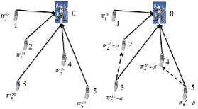
Figure 1: Direct Transmission and BE enabled Incentivized Forwarding

II System Model

We consider the uplink of an $N$ node single cell FDMA network. Let $\mathcal{V}=\{1,\,2,\,\cdots,\,N\}$ denote the set of $N$ nodes that transmit data to the BS (node $0$). Each node uses the total time slot. Node $i\,\in\,\mathcal{V}$ is initially allotted a bandwidth of $W_{i}^{in}$. Let $\rho_{ij}$ and $R_{ij}$ denote the link gain and achievable rate of the $ij$ path respectively. For a given node $i\in[1,N]$ with $W_{i}^{in}$ bandwidth and direct link gain $\rho_{i0}$, the achievable throughput is:

$$R_{i}^{in}=R_{i0}=W_{i}^{in}\log_{2}\bigl{(}1+\frac{\rho_{ij}P_{i,max}}{W_{i}^{in}}\bigr{)}$$ (1)

Here, $P_{i,max}$ denotes the maximum transmission power of node $i$ and $R_{i}^{in}$ is expressed in bit per second (bps).

In BE, nodes perform two hop half duplex DF cooperative relaying. The forwarder node hears the sender nodes’ data and relays some of that data along with transmitting its own data to the AP. Since each node is a power constrained device, the forwarder nodes’ data rate may drop if it continues to transmit with the same bandwidth. Therefore, the sender node delegates some of its bandwidth to the forwarder node as incentives for relaying. We consider one forwarder for one sender and vice versa to reduce the relay searching complexity. Let $\mathcal{SF}=\{\mathcal{SF}_{1},\cdots,\mathcal{SF}_{K}\}=\{(s_{1},f_{1}),(s_{2},f_{2}),\cdots,(s_{K},f_{K})\}$ denote the sender-forwarder pair set, i.e., $f_{i}$ relays $s_{i}$’s data along with transmitting $f_{i}$’s own data. Let $\mathcal{D}={d_{1},d_{2},\cdots,d_{L}}$ denote the direct set, i.e., the set of remaining nodes that transmit data without cooperation. Note that, $K$ and $L$ are variables and further, $2*K+L=N$. We assume pairwise bandwidth constraint in this work.

The left and right sides of Fig. 1 show the considered direct transmission model and the proposed BE model. In BE, node $2$ relays data for node $3$. Node $3$ delegates $\alpha$ amount of bandwidth to node $2$ as incentive for relaying. Let $W_{i}^{be}$ represent the bandwidth of node $i$ in the BE scenario. Now, $W_{2}^{be}=W_{2}^{in}+\alpha$ and $W_{3}^{be}=W_{3}^{in}-\alpha$. Node $4$ and $5$ operate in the same manner.

Nodes don’t do power allocation among different streams in our framework. Since capacity is a non-decreasing function of transmission power, each node utilizes the maximum transmission power in its allotted bandwidth slot. Without loss of generality, we assume $P_{i,max}=P\,\forall\,i\,\in\,\mathcal{V}$ in the subsequent analysis.

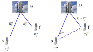
Figure 2: BE Enabled Forwarding in a $3$ Node Network

II-1 Rate analysis in the BE scenario:

TABLE I: Summary of used notations

Notation	Meaning
$N$	Total number of users
$P$	Maximum transmission power
$\rho_{ij}$	Gain of the $ij$ link
$W_{i}^{in}$	Initial bandwidth of node $i$
$W_{i}^{be}$	Node $i$’s bandwidth in BE
$R_{i}^{in}$	Initial rate of node $i$
$R_{i}^{be}$	Node $i$’s rate in BE
$R_{ij}$	Achievable rate in the $ij$ link
$\mathcal{V}$	Set of all nodes
$\mathcal{D}$	Set of nodes that transmit without cooperation
$\mathcal{SF}$	Set of sender-forwarder pairs
$SF_{i}$	$i^{th}$ sender-forwarder pair $(s_{i},f_{i})$

Let $R_{i}^{be}$ represent the achievable rate of node $i$ in the BE scenario. The right side of Fig. 2 shows the interaction between a sender node $s$ and a forwarder node $f$. If node $s$ transmits to node $f$ and the BS separately using $W_{s}^{be}$ bandwidth, the achievable throughput in the respective paths are:

$$R_{sf} = W_{s}^{be}\log_{2}\bigl{(}1+\frac{\rho_{sf}P}{W_{s}^{be}}\bigr{)}$$ (2)

$$R_{s0} = W_{s}^{be}\log_{2}\bigl{(}1+\frac{\rho_{s0}P}{W_{s}^{be}}\bigr{)}$$ (3)

If $f$ transmits to the BS using $W_{f}^{be}$ bandwidth,

$$R_{f0}=W_{f}^{be}\log_{2}\bigl{(}1+\frac{\rho_{f0}P}{W_{f}^{be}}\bigr{)}$$ (4)

Assuming $\rho_{sf}\geq\rho_{s0}$, it is easily seen that $R_{sf}\geq R_{s0}$. Due to the nature of the wireless environment, when sender $s$ transmits, both $f$ and BS hear it. If node $s$ transmits at rate $R_{sf}$, node $f$ can decode it properly. The BS also receives the same signal but can’t decode it properly since $R_{sf}\geq R_{s0}$. However, node $f$ can forward $R_{c}$ bits to the BS to resolve the BS’s uncertainty about node $s$’s data. Node $f$ also transmits its own data, $R_{f}^{be}$, to the BS. The information theoretic generalization of the maximum-flow-minimum-cut-theorem [19] provides the following relationship between these achievable rates,

$$R_{s}^{be} \leq \min(R_{sf},R_{s0}+R_{c})$$ (5)

$$R_{c}+R_{f}^{be} \leq R_{f0}$$ (6)

The codebook design procedure to achieve these rates is summarized in Appendix A. A detailed description can be found in [19, 20].

Using this rate analysis, we focus on the distributed joint optimal bandwidth allocation and relay selection in maximizing the summation of the $\alpha$-fair utilities of the network.

$\alpha$-fair utility:

The $\alpha$-fair utility is defined for any $\alpha\,\in\,[0,\infty)$, as [21],

$$U^{\alpha}(R)=\begin{cases}\frac{R^{1-\alpha}}{1-\alpha},&\text{if \, $\alpha\neq 1$}\\ log(R),&\text{if \, $\alpha=1$}\end{cases}$$ (7)

where $R$ represents the rate of the user. Summation of $\alpha$-fair utility functions takes the form of different well known utility functions, e.g., sum rate maximization ($\alpha=0$), proportional fairness ($\alpha=1$) and minimum rate maximization ($\alpha=\infty$).

III Design Objective

We begin with a focus on $\alpha$-fair NUM of the overall network through optimal bandwidth and rate allocation for all possible sender-forwarder pairing sets.

Problem I

$$\mathbf{\max.}\,\sum_{d\in\mathcal{D}}U^{\alpha}(R_{d}^{be})+\sum_{(s,\,f)\in\mathcal{SF}}\bigl{(}U^{\alpha}(R_{f}^{be})+U^{\alpha}(R_{s}^{be})\bigr{)}$$ (8a)

$$\mathbf{s.t.}\,\,(R_{f}^{be},R_{s}^{be})\,\in\,conv(W_{f}^{be},W_{s}^{be})\,\,\forall\,(s,f)\,\in\,\mathcal{SF}$$ (8b)

$$R_{f}^{be}\geq R_{f}^{in}\,,\,R_{s}^{be}\geq R_{s}^{in}\,\,\forall\,(s,f)\,\in\,\mathcal{SF}$$ (8c)

$$W_{f}^{be}+W_{s}^{be}\,\leq\,W_{f}^{in}+W_{s}^{in}\,\,\forall\,(s,f)\,\in\,\mathcal{SF}$$ (8d)

$$\,\,W_{f}^{be},\,W_{s}^{be}\,\geq 0\,\,\forall\,(s,f)\,\in\,\mathcal{SF}$$ (8e)

$$\mathcal{D}\subseteq\mathcal{V}\,,\,\mathcal{SF}\in\mathcal{V}\times\mathcal{V}\,\,,\,\,\mathcal{SF}_{i}\cap\mathcal{SF}_{j}=\emptyset\,\,\forall i\neq j$$ (8f)

$$\mathcal{SF}_{i}\cap\mathcal{D}=\emptyset\,\forall\,i\,\in[1,K]$$ (8g)

$$\mathcal{SF}_{1}\cup\mathcal{SF}_{2}\cdots\cup\mathcal{SF}_{K}\cup\mathcal{D}=\mathcal{V}$$ (8h)

$$Variables\,\,\mathcal{D},\mathcal{SF},R_{s}^{be},R_{f}^{be},W_{s}^{be},W_{f}^{be}$$

Here, $R_{d}^{be}=R_{d}^{in}\,\forall\,d\,\in\,D$. Therefore, the rates of the direct node set are not optimization variables. Equation (8b) denotes that the rate of the sender and forwarder lie in the convex hull of the allocated bandwidth. The details of this convex hull has already been explained in the system model. It will also be mentioned in the next section. Eq. (8c) represents that the sender and the forwarders’ rate cannot drop below their initial rates. Equation (8d) shows that the total bandwidth used by the cooperative pair is constrained by the summation of the initial bandwidths allocated to the individual nodes. Equation (8f)- (8h) represent the relay selection constraints. Equation (8f) shows that the direct and sender-forwarder sets are all subsets of the overall set. Eq. (8g) denotes that the sender-forwarder pairs and direct set cannot have any common nodes. Eq. (8h) represents that the union of the pairs and the direct set form the overall set $\mathcal{V}$.

The solution of the above optimization problem depends on the selected sender-forwarder and direct node set and the corresponding bandwidth and rate allocations. Hence, it involves an exponential number of variables and constraints. In the rest of the paper, we focus on solving this problem.

IV Optimization Problem Solution

IV-A Modified Optimization Problem

Let $U^{\alpha}(R_{tot})=\sum_{i\in\mathcal{V}}U^{\alpha}(R_{i}^{in})$ denote the summation of the initial utilities of the nodes. For a fixed $\mathcal{SF}$, $U^{\alpha}(R_{tot})$ can be expressed in the following form:

$$U^{\alpha}(R_{tot})$$ (9)

$$= \sum_{i\in\mathcal{V}}U^{\alpha}(R_{i}^{in})$$

$$= \sum_{d\in\mathcal{D}}U^{\alpha}(R_{d}^{in})+\sum_{(s,\,f)\in\mathcal{SF}}\bigl{(}U^{\alpha}(R_{f}^{in})+U^{\alpha}(R_{s}^{in})\bigr{)}$$

$$= \sum_{d\in\mathcal{D}}U^{\alpha}(R_{d}^{be})+\sum_{(s,\,f)\in\mathcal{SF}}\bigl{(}U^{\alpha}(R_{f}^{in})+U^{\alpha}(R_{s}^{in})\bigr{)}$$ (10)

Equation (9) follows from eq. (8h). Equation (10) uses the fact that $R_{d}^{be}=R_{d}^{in}\,\forall\,d\in D$. Subtracting $U^{\alpha}(R_{tot})$ from the objective function of I, we find the following optimization problem:

Problem II

$$\sum_{(s,\,f)\in\mathcal{SF}}\bigl{(}U^{\alpha}(R_{f}^{be})+U^{\alpha}(R_{s}^{be})-U^{\alpha}(R_{f}^{in})+U^{\alpha}(R_{s}^{in})\bigr{)}$$ (11a)

$$\mathbf{s.t.}\,\,(R_{f}^{be},R_{s}^{be})\,\in\,conv(W_{f}^{be},W_{s}^{be})\,\,\forall\,(s,f)\,\in\,\mathcal{SF}$$ (11b)

$$R_{f}^{be}\geq R_{f}^{in}\,,\,R_{s}^{be}\geq R_{s}^{in}\,\,\forall\,(s,f)\,\in\,\mathcal{SF}$$ (11c)

$$W_{f}^{be}+W_{s}^{be}\,\leq\,W_{f}^{in}+W_{s}^{in}\,\,\forall\,(s,f)\,\in\,\mathcal{SF}$$ (11d)

$$\,\,W_{f}^{be},\,W_{s}^{be}\,\geq 0\,\,\forall\,(s,f)\,\in\,\mathcal{SF}$$ (11e)

$$\mathcal{D}\subseteq\mathcal{V}\,,\,\mathcal{SF}\in\mathcal{V}\times\mathcal{V}\,\,,\,\,\mathcal{SF}_{i}\cap\mathcal{SF}_{j}=\emptyset\,\,\forall i\neq j$$ (11f)

$$\mathcal{SF}_{i}\cap\mathcal{D}=\emptyset\,\forall\,i\,\in[1,K]$$ (11g)

$$\mathcal{SF}_{1}\cup\mathcal{SF}_{2}\cdots\cup\mathcal{SF}_{K}\cup\mathcal{D}=\mathcal{V}$$ (11h)

$$Variables\,\,\mathcal{D},\mathcal{SF},R_{s}^{be},R_{f}^{be},W_{s}^{be},W_{f}^{be}$$

The inclusion of constant terms in the objective function does not change the optimal variables of an optimization problem [22]. As a result, the same set of sender-forwarder pairs maximize both problem I and II. We will focus on solving problem II in the subsequent analysis. The optimal variables of problem II will directly lead to the optimal solution of problem I.

Problem II depends on both relay selection and resource allocation. The very nature of the design objective allows us to split the optimization formulation into the following two parts:

• For any fixed set of sender-forwarder pairs, perform DF based optimal rate and bandwidth allocation.

• Choose the relay set that maximizes the summation of the $\alpha$-fair utility of the nodes.

We, at first, focus on resource allocation in a fixed sender-forwarder pair set $\mathcal{SF}$ and direct node set $\mathcal{D}$. Later, we will show the optimal sender-forwarder pair selection policy.

IV-B Optimal bandwidth and rate allocation for a fixed sender-forwarder set

The optimal resource allocation problem for fixed $\mathcal{SF}$ and $\mathcal{D}$ takes the following form:

Problem III

$$\sum_{(s,\,f)\in\mathcal{SF}}\bigl{(}U^{\alpha}(R_{f}^{be})+U^{\alpha}(R_{s}^{be})-U^{\alpha}(R_{f}^{in})-U^{\alpha}(R_{s}^{in})\bigr{)}$$ (12a)

$$\mathbf{s.t.}\,(R_{f}^{be},R_{s}^{be})\,\in\,conv(W_{f}^{be},W_{s}^{be})\,\,\forall\,(s,f)\,\in\,\mathcal{SF}$$ (12b)

$$R_{f}^{be}\geq R_{f}^{in}\,\,,\,\,R_{s}^{be}\geq R_{s}^{in}\,\,\,\forall\,(s,f)\,\in\,\mathcal{SF}$$ (12c)

$$W_{f}^{be}+W_{s}^{be}\,\leq\,W_{f}^{in}+W_{s}^{in}\,\,,\,\,W_{f}^{be},\,W_{s}^{be}\,\geq 0\,\,\forall\,(s,f)\,\in\,\mathcal{SF}$$ (12d)

$$Variables\,\,R_{s}^{be},\,R_{f}^{be},\,W_{s}^{be},\,W_{f}^{be}$$ (12e)

Now, due to the pairwise bandwidth constraint of (12d), the bandwidth allocation in one cooperative pair does not affect other nodes. Therefore, problem III is just the summation of $K$ independent three node (sender, forwarder and BS) resource allocation problems and can be decomposed into the subproblems. Hence, we now focus on an arbitrary sender-forwarder pair $(s,f)$ and describe the resource allocation problem formulation in this pair.

Problem IV

$$\mathbf{\max.}\,\,U^{\alpha}(R_{f}^{be})+U^{\alpha}(R_{s}^{be})-U^{\alpha}(R_{f}^{in})-U^{\alpha}(R_{s}^{in})$$ (13a)

$$\mathbf{s.t.}\,\,R_{sf}\leq W_{s}^{be}\log_{2}\bigl{(}1+\frac{P*\rho_{sf}}{W_{s}^{be}}\bigr{)}$$

$$R_{s0}\leq W_{s}^{be}\log_{2}\bigl{(}1+\frac{P*\rho_{s0}}{W_{s}^{be}}\bigr{)}$$

$$R_{c}+R_{f}^{be}\leq W_{f}^{be}\log_{2}\bigl{(}1+\frac{P*\rho_{f0}}{W_{f}^{be}}\bigr{)}$$ (13b)

$$R_{s}^{be}\leq\min(R_{sf},R_{s0}+R_{c})\,,\,R_{f}^{be}\geq R_{f}^{in}\,,\,R_{s}^{be}\geq R_{s}^{in}$$ (13c)

$$W_{f}^{be}+W_{s}^{be}\,\leq\,W_{f}^{in}+W_{s}^{in}\,\,,\,\,W_{f}^{be},\,W_{s}^{be}\,\geq 0\,\,\forall\,(s,f)\,\in\,\mathcal{SF}$$ (13d)

$$Variables\,\,\,R_{s}^{be},R_{f}^{be},W_{s}^{be},W_{f}^{be},R_{c}$$

Equation (13b) and (13c) show the convex hull of the allotted bandwidths and the achievable rates. They have also already been described in the system model.

Lemmma 1: Problem IV is a concave maximization problem.

Proof: $U^{\alpha}(R_{f}^{in})$ and $U^{\alpha}(R_{s}^{in})$ are the utilites of the initial data rates and constants, in terms of the optimization variables. The concavity of $\alpha$-fair utility functions and the capacity expressions can be easily shown [22]. The minimum of linear (concave) functions is concave. Thus, the objective function is concave and the constraints are convex or linear in terms of the optimization variables. This proves the concavity of Problem IV. $\blacksquare$.

Problem IV can be solved using standard convex optimization algorithms, e.g., interior point methods [22].

Lemma 2: $(R_{s}^{be},R_{f}^{be},W_{s}^{be},W_{f}^{be},R_{c})=(R_{s}^{in},R_{f}^{in},W_{s}^{in},W_{f}^{in},0)$ is a feasible set of variables of Problem IV.

Proof: Let $W_{f}^{be}=W_{f}^{in}$, $W_{s}^{be}=W_{s}^{in}$, $R_{c}=0$. Then,

$$R_{sf}=W_{s}^{in}\log_{2}\bigl{(}1+\frac{P*\rho_{sf}}{W_{s}^{in}}\bigr{)}$$

$$R_{s0}=W_{s}^{in}\log_{2}\bigl{(}1+\frac{P*\rho_{s0}}{W_{s}^{in}}\bigr{)}=R_{s}^{in}$$ (14)

$$R_{f}^{be}=W_{f}^{in}\log_{2}\bigl{(}1+\frac{P*\rho_{f0}}{W_{f}^{in}}\bigr{)}=R_{f}^{in}$$

$$R_{s}^{be}=\min(R_{sf},R_{s0}+R_{c})=\min(R_{sf},R_{s0})=R_{s}^{in}$$

This is a feasible solution of problem IV. $\blacksquare$

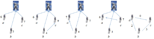
Figure 3: MWM in BE Enabled Relay Network

Thus, if Node $s$ and $f$ use their initial bandwidths and if the forwarder $f$ does not relay any data of the sender $s$, both sender and forwarder will continue to transmit at their initial rates. The corresponding feasible solution for these variables can be found as follows,

$$U^{\alpha}(R_{f}^{be})+U^{\alpha}(R_{s}^{be})-U^{\alpha}(R_{f}^{in})-U^{\alpha}(R_{s}^{in})$$

$$=U^{\alpha}(R_{f}^{in})+U^{\alpha}(R_{s}^{in})-U^{\alpha}(R_{f}^{in})-U^{\alpha}(R_{s}^{in})=0$$

Since, problem IV is a concave maximization probelm, the optimal solution will not drop below $0$ [22]. Hence, the proposed BE enabled relaying scheme will perform at least as good as the initial allocation and seek to maximize the global utility while preserving the initial rates of the individual nodes.

Lemma 3: Problem III is a concave maximization problem.

Proof: Problem III is the combination of $K$ disjoint concave maximization problems and hence it’s concave. $\blacksquare$

IV-C Optimal sender-forwarder set selection

Let $g_{sf}^{*}$ denote the solution of problem IV, i.e., the optimal gain obtained through cooperation of $(s,\,f)$. Let, $U_{\mathcal{D},\mathcal{SF}}^{*}$ represent the optimal solution of problem III, i.e., the optimal cooperation gain for the selected sender-forwarder pair set $\mathcal{SF}$. Then, $U_{\mathcal{D},\mathcal{SF}}^{*}=\sum_{(s,\,f)\in\mathcal{SF}}g_{sf}^{*}$. Therefore, the sender-forwarder pairing set selection part of problem II is equivalent to finding the set of pairs that maximize the gain in utility through cooperation, over noncooperation. It can be written in the following form:

Problem V

$$\mathbf{\arg\max_{\mathcal{SF}}}\sum_{(s,\,f)\in\mathcal{SF}}g_{sf}^{*}$$ (15a)

$$\mathcal{SF}\in\mathcal{V}\times\mathcal{V}\,\,,\,\,\mathcal{SF}_{i}\cap\mathcal{SF}_{j}=\emptyset\,\,\forall i\neq j\,,\,$$ (15b)

Now, consider a graph $\mathcal{G}=(\mathcal{V},\mathcal{E})$ where the vertices $\mathcal{V}$ represent the set of $N$ nodes under consideration and $\mathcal{E}$ denote the edges between these nodes. Define the edge weight of any $(i,j)$ pair by $U^{\alpha}(R_{i}^{be})+U^{\alpha}(R_{j}^{be})-U^{\alpha}(R_{i}^{in})-U^{\alpha}(R_{j}^{in})$, i.e., the difference, in terms of utility, between the cooperation and non-cooperation scenario. The optimal sender-forwarder pairing set selection of problem V is equivalent to finding the set of pairs that maximize the difference between cooperation and noncooperation utility. Hence, the optimal sender-forwarder pair selection problem can be reduced to the problem of finding the set of pairs that maximizes the link weights mentioned above. Thus, the optimal relay selection converges to the classical nonbipartite MWM problem. The nonbipartite MWM algorithm has been summarized in Appendix B. A detailed description can be found in [7].

Fig. 3 illustrates the application of MWM in the sender-forwarder pairing selection. The left figure of Fig. 3 denote the initial scenario where node $a$, $b$ and $c$ transmit through the direct path and transmit $6$, $3$ and $7$ bits respectively. The three figures in the middle show the obtained rates for different sender-forwarder pair selection. The second figure from the left shows that $b$ and $c$ transmit $4$ and $9$ bits respectively through BE enabled DF cooperation. Thus, the utility gain of cooperation, over noncooperation, is $3$ bits. The middle figure and the 2nd figure from the right represent the cooperation scenarios of $(a,b)$ and $(a,c)$ respectively. The rightmost figure represents the edge weights of each cooperative pair in terms of the utility gain of cooperation, over noncooperation. The MWM algorithm will select node $(b,c)$ as the cooperative pair and node $a$ will transmit without cooperation.

Centralized nonbipartite MWM can be solved optimally in $O(N^{3})$ time [7]. Our proposed distributed incentivized forwarding is based on the distributed local greedy MWM [8] $(O(N^{2}))$ and is described below. The distributed MWM algorithm [8] is summarized in Appendix C.

IV-D Distributed BE incentivized forwarding protocol

• Focus on an arbitrary node, node $v$. Node $v$ sends training symbols to the AP and obtains its own direct channel, $\rho_{v0}$, through feedback. Node $v$ is initially allocated $W_{v}^{in}$ bandwidth and transmits at $R_{v}^{in}$ rate.

• Let node $u$ be a neighbouring node of $v$. Due to the nature of wireless channels, node $u$ receives node $v$’s channel estimation training symbols and finds the inter-node channel gain, $\rho_{uv}$.

• $v$ sends an omnidirectional signal containing $\rho_{v0}$, $W_{v}^{in}$ and $R_{v}^{in}$ to the neighbouring nodes.

• Node $u$ may relay node $v$’s data if $min(\rho_{uv},\rho_{u0})\geq\rho_{v0}$. Thus, $v$ knows its potential forwarders or senders.

• $v$ solves problem IV for the suitable neighbours. Thus, each node knows its adjacent link weights.

• $v$ solves the distributed local greedy MWM algorithm of [8].

• The ‘matched pairs’ allocate resources among themselves. The ‘unmatched’ nodes transmit without cooperation.

IV-E Outage probability reduction in BE

We define outage probability as the ratio of the number of nodes that do not get minimum data rate to the total number of nodes. We assume that each node in the network starts with an initial amount of resource. Depending on the resource and link gains, nodes fall in the following two groups:

• Outage group: Node that cannot meet the minimum required rate with initially allocated resources.

• Non-Outage group: Node that can meet the minimum rate with initially allocated resources.

The outage probability reduction problem can be defined as providing minimum data rate to the most number of users in the outage group, while maintaining the minimum data rate of the nodes, in the non-outage group. MWM based matching and pairwise resource allocation based incentivized two-hop forwarding can help in this case. We propose the following scheme in this regard:

• Each node in the outage group solves the pairwise sumrate maximization, with minimum rate constraints, for each of its neighbouring node. Nodes can solve sumrate maximization by plugging $\alpha=0$ in the $\alpha$-fair utility function.

• If the node in outage can maintain minimum data rate by pairing with the forwarder, i.e., the non-outage node, we assume that an edge exists between these nodes.

• The relay selection problem in outage probability reduction becomes maximizing the number of edges in the network. This reduces to the maximum matching (MM) algorithm in a bipartite graph [23].

Our focus here is to maximize the number of users that receive minimum data rate, not to maximize any utility function. That’s why, we use MM, instead of MWM, in this part of the work. Besides, cooperation between two nodes in the non-outage group do not change the outage probability of the network. Therefore, we consider a bipartite graph by dividing the graph into outage and non-outage group.

V Numerical Simulations

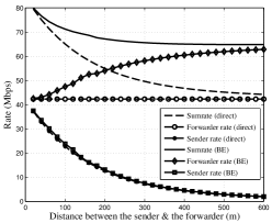
Figure 4: Sumrate Maximization in a 3 Node Network, $10$ MHz per Node, $P$ = $100$ mW, Near node-AP distance = 150m

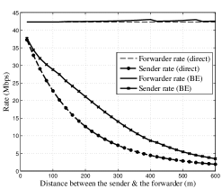
Figure 5: Minimum Rate Maximization in a 3 Node Network, $10$ MHz per Node, $P$ = $100$ mW, Near node-AP distance = 150m

We assume equal initial bandwidth allocation in all of our simulations, i.e., nodes start with equal bandwidth. However, our work is readily applicable to the scenario where nodes start with optimal bandwidth allocation (based on direct path transmission) and then use bandwidth as incentives for two hop relaying.

Fig. 4 and Fig. 5 compare the performance of BE relaying with that of direct path transmission in the sumrate maximization and minimum rate maximization of a $3$ node network (sender, forwarder and BS). Both sender and forwarder initially receive 10 MHz bandwidth and transmit uplink data to the BS. The forwarder node is placed in the straight line that connects the BS and the sender node. The distance between the forwarder node and the BS is kept fixed at $150$m, whereas, the distance between the BS & the sender node is varied. In these two simulations, we assumed the link gains to take the form, $\rho_{ij}=kd_{ij}^{-3}$ where $d_{ij}$ is the distance between the $i^{\mathrm{th}}$ and $j^{\mathrm{th}}$ node. $k$ is the proportionality constant that also captures the noise spectral density and is set to $k=6\times 10^{6}MHz*m^{3}/mW$ [6].

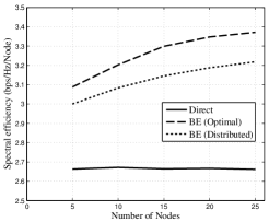
Figure 6: Spectrum Efficiency in an $N$ Node Network, $1$ MHz per Node, $P$ = $20$ dBm

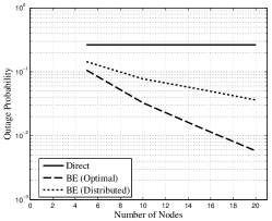
Figure 7: Outage Probability in an $N$ Node Network, $1$ MHz per Node, $P$ = $20$ dBm

The sumrate maximization objective based plot of Fig. 4 shows that BE relaying improves the rate of the forwarder (near user) while ensuring that the sender’s (far user) rate does not drop below its initial value. This increase in the forwarders’ rate gets reflected in the sumrate gain of the network. On the other hand, the minimum rate maximization objective based plot of Fig. 5 shows that BE relaying improves the senders’ (far user) rate while ensuring that the forwarders’ (near user) rate does not drop. This diverse contribution of BE relaying comes from the problem objectives of the respective simulations; sumrate maximization ($\alpha=0$) is the most efficient allocation whereas minimum rate maximization ($\alpha=\infty$) is the most fair one. Therefore, the use of any $\alpha\in(0,\infty)$ would have increased both users’ rates in this simulation scenario.

Fig. 6 and Fig. 7 show the performance of BE relaying in an $N$ node network. In these simulations, we assumed that links are under independent Rayleigh fading and the link gain in each slot is an independent realization of Rayleigh random variable. This means that the link gain, $\rho_{ij}$, is exponentially distributed, $p(\rho_{ij})=\frac{1}{\bar{\rho}_{ij}}exp\bigl{(}-\frac{\rho_{ij}}{\bar{\rho}_{ij}}\bigr{)}$ where $\bar{\rho}_{ij}=kd_{ij}^{-3}$ and $k=6\times 10^{6}MHz*m^{3}/mW$. We consider a circular cell of $800m$ radius. The AP is located at the center, whereas, the nodes are placed randomly in the cell. We considered transmission scheme much like the one used in mobile Wimax. Each node is preassigned 20 dBm transmit power and 1 MHz bandwidth. We used the matching code of [24] to implement the MWM algorithm in Matlab.

We showed the performance of both centralized and distributed algorithms in Fig. 6 and Fig. 7. In the simulation of the distributed algorithm, we assumed that each node can only talk to its neighbours that are located within $500$m from the sender node. Fig. 6 shows that the centralized and decentralized algorithm improves the spectral efficiency by 25% and 20% respectively. The performance of the distributed algorithm will improve if we allow each node to talk to neighbours with greater distances.

Fig. 7 shows that BE enabled relaying provides cooperative diversity and significantly reduces the outage probability (90-98%). Thus, BE can be used to extend the coverage in an autonomous network.

VI Discussion

In this paper, we considered joint optimal relay selection and resource allocation in the $\alpha$-fair NUM and outage probability reduction of a BE network. Our proposed resource allocation formulation maximizes the global utility of the cooperative pair while preserving the initial utilities of each individual node. We showed that the relay selection part of the $\alpha$-fair NUM problem reduces to the nonbipartite matching algorithm. Numerical simulations suggest that the proposed BE enabled relaying provides 20-25% spectrum efficiency gain and 90-98% outage probability reduction in a $20$ node network.

Our work can be really advantageous in the following scenario: the nodes start with a direct path based centrally allocated optimal resources. Thereafter, nodes employ the proposed algorithm to improve the system performance through distributed relay selection and pairwise resource allocation. This scheme saves a huge amount of signalling overhead, an inherent drawback of centralized optimal two hop forwarding, at the cost of lower performance.

The proposed algorithm considers one forwarder for one sender and vice versa. The generalization of this algorithm to the multiple sender-forwarder scenario is an area of future research. We also plan to focus on discrete subcarrier exchange in our future works.

VII Acknowledgements

This work is supported by the Office of Naval Research under grant N00014-11-1-0132. We thank Vladimir Oudalov and Dr. Mung Chiang for their insights on maximum weighted matching algorithm. We are also grateful to Joris V. Rantwijk for the MWM implementation code [24].

Appendix A Codebook Design in Proposed DF Relaying

Let’s consider two codebooks $\mathcal{W}$ and $\mathcal{C}$ that consist of $2^{R_{sf}}$ and $2^{R_{c}}$ codewords respectively. Assume, $\mathcal{W}=\{w_{1},w_{2},\cdots,w_{2^{R_{sf}}}\}$ and $\mathcal{C}=\{c_{1},c_{2},\cdots,c_{2^{R_{c}}}\}$. Here $R_{sf}\geq R_{c}$. Consider a partition $\mathcal{S}=\{S_{1},S_{2},\cdots,S_{2^{R_{c}}}\}$ of $\mathcal{W}$, i.e., $\mathcal{W}$ has been partitioned into $2^{R_{c}}$ cells. Each cell $S_{i}$ contains $2^{R_{sf}-R_{c}}$ codewords of $\mathcal{W}$. Assume a one-to-one correspondence between $\mathcal{C}$ and $\mathcal{S}$, i.e., each codeword of $\mathcal{C}$ represents one particular cell of $\mathcal{S}$.

The BS (node $0$), sender $s$ and forwarder $f$ get the codebooks off-line. At the beginning of transmission, sender $s$ sends a codeword $w_{i}$ from $\mathcal{W}$ using $R_{sf}$ bits. The forwarder node decodes the codeword correctly. However, since $R_{sf}\geq R_{s0}$, the BS cannot decode it correctly. The BS has a list of possible codewords of size $2^{R_{sf}-R_{s0}}$. Now, the forwarder $f$ finds the cell $S_{i}$ where $w_{i}$ lies and sends $c_{i}$ using $R_{c}$ bits. The BS receives $c_{i}$ and intersects $S_{i}$ with the list of possible codewords. If $R_{c}\geq R_{sf}-R_{s0}$ and $R_{c}\leq R_{f0}$, this half duplex DF cooperation completely removes the BS’s uncertainty about $w_{i}$ [20, 19].

Thus, the achievable rates of node $s$ and $f$ are governed by this information theoretic generalization of the max-flow-min-cut theorem:

$$R_{s}^{be} \leq \min(R_{sf},R_{s0}+R_{c})$$

$$R_{c}+R_{f}^{be} \leq R_{f0}$$

Appendix B Matching and nonbipartite MWM algorithm

Consider an undirected graph $\mathcal{G}=(\mathcal{V},\mathcal{E})$ where $\mathcal{V}$ denotes the set of vertices and $\mathcal{E}$ denotes the set of edges. A matching $\mathcal{M}$ is a subset of $\mathcal{E}$ such that $e_{1}\cap e_{2}=\emptyset$ for $e_{1},e_{2}\in\mathcal{M}$ if $e_{1}\neq e_{2}$ [23].

Let $x_{e}$ denote whether an edge $e\in E$ will be selected in the matching, i.e., $x_{e}$ can be $0$ or $1$. Let $r_{e}$ represent the edge weights. The maximum weighted matching in a non-bipartite graph takes the following form [23]:

$$\mathbf{max}\sum_{e\in E}r_{e}x_{e}$$ (16a)

$$\mathbf{s.t.}\sum_{e\in\delta(v)}x_{e}\leq 1\,\forall\,v\,\in\,\mathcal{V}$$ (16b)

$$\sum_{e\in E(\mathcal{U})}x_{e}\leq\lfloor\frac{|\mathcal{U}|}{2}\rfloor\,\forall\,\,odd\,sets\,\,\mathcal{U}\subset\mathcal{V}$$ (16c)

$$x_{e}\in\mathcal{B}^{n}$$ (16d)

In (16b), $\delta(v)$ denotes the edges connected with node $v$. In (16c), $E(\mathcal{U})$ represents the edges contained in the set $\mathbf{U}$. Equation (16d) shows that $x_{e}$ takes Boolean values. However, Edmonds [7] showed that the we can replace $x_{e}\in\mathcal{B}^{n}$ by $x_{e}\in\mathcal{R}^{n}_{+}$ and still obtain integral optimal solutions. Thus the combinatorial optimization can be converted to a linear program.

Appendix C Distributed Local Greedy MWM

• Each node $i$ knows its adjacent link weights. Node $i$ picks the “candidate” node $j$, based on the heaviest link weight and sends an “add” request.

• Wait for the response from node $j$.

• If node i receives an “add” request from node $j$, $i$ and $j$ pick each other as the cooperative pair. $i$ sends “drop” request to its other neighbouring nodes.

• If node i receives a “drop” request from node $j$, node $i$ removes the $(i,j)$ link from its adjacent edge set. Node $i$ goes to the state of step $1$.

The distributed local greedy MWM provides at least 50% performance of centralized optimal matching. Distributed local greedy MWM requires $O(N^{2})$ amount of message passing.

References

- [1] J. N. Laneman, D. N. C. Tse, and G. Wornell, “Cooperative diversity in wireless networks : efficient protocols and outage behavior,” IEEE Trans. Info. Theory, vol. 50(12), pp. 3062–3080, Dec. 2004.
- [2] L. Lai, K. Liu, and H. El Gamal, “The three node wireless network: Achievable rates and cooperation strategies,” IEEE Trans. Info. Theory, vol. 52(3), pp. 805–828, Mar. 2006.
- [3] O. Ileri, S.-C. Mau, and N. Mandayam, “Pricing for enabling forwarding in self-configuring ad hoc networks,” IEEE JSAC, vol. 23, pp. 151–162, Jan. 2005.
- [4] S. Buchegger and J.-Y Le Boudec, “Self-policing mobile ad hoc networks by reputation systems,” IEEE Communication Magazine, vol. 43, pp. 101–107, July 2007.
- [5] M. Felegyhazi, J. P. Hubaux, and L. Buttyan, “Nash equilibria of packet forwarding strategies in wireless ad hoc networks,” IEEE Trans. on Mobile Computing, vol. 5, pp. 463–475, May 2006.
- [6] D. Zhang, R. Shinkuma, and N. B. Mandayam, “Bandwidth exchange: An energy conserving incentive mechanism for cooperation,” IEEE Trans. Wireless Comm, vol. 9(6), pp. 2055–2065, June 2010.
- [7] J. Edmonds, “Paths, trees and flowers,” Canadian Journal of Mathematics, vol. 17, pp. 449–467, 1965.
- [8] J. Hoepman, “Simple distributed weighted matchings,” eprint, October 2004, http://arxiv.org/abs/cs/0410047.
- [9] J. Zhang and Q. Zhang, “Stackelberg game for utility-based cooperative cognitive radio networks,” in Proc. ACM MOBIHOC’2009, May 2009, pp. 23–31.
- [10] H. Xu and B. Li, “Efficient resource allocation with flexible channel cooperation in ofdma cognitive radio networks,” in Proc. IEEE INFOCOM’2010, Mar. 2010, pp. 1–9.
- [11] M. N. Islam, N. B. Mandayam, and S. Komplella, “Optimal resource allocation in a bandwidth exchange enabled relay network,” in Proc. IEEE MILCOM’2011, Nov. 2011.
- [12] C. T. K. Ng and G. J. Foschini, “Transmit signal and bandwidth optimization in multiple-antenna relay channels,” IEEE Trans. Wireless Comm., vol. 59, pp. 2987–2992, Nov. 2011.
- [13] L. Tassiulas and A. Ephremides, “Stability properties of constrained queing systems and scheduling for maximum throughput in multihop radio networks,” IEEE Trans. Automatic Control, vol. 37(12), pp. 1936–1949, Dec. 1992.
- [14] M. J. Neely, E. Modiano, and C. E. Rohrs, “Dynamic power allocation and routing for time-varying wireless networks,” IEEE Journal on Selected Areas in Communications, vol. 23(1), pp. 89–104, Jan. 2005.
- [15] S. Sarkar and L. Tassiulas, “End-to-end bandwidth gurantees through fair local spectrum share in wireless ad-hoc networks,” in Proc. IEEE Conference on Decision and Control, Dec. 2011.
- [16] Y. Yi and M. Chiang, “Stochastic network utility mazmimization and wireless scheduling,” in Next Generation Internet Architectures and Protocols, B. Ramamurthy, G. Rouskas, and K. Sivalingam, Eds., pp. 1–35. Cambridge University Press, New York, 2011.
- [17] X. Lin and N. B. Shroff, “The impact of imperfect scheduling on cross-layer rate control in wireless networks,” in Proc. IEEE INFOCOM 2005, Mar. 2005.
- [18] V. Mahinthan, J. Mark L. Cai, and X. Shen, “Maximizing cooperative diversity energy gain for wireless networks,” IEEE Trans. Wireless Comm, vol. 7(6), pp. 2540–2549, 2007.
- [19] T. Cover and H. El Gamal, “Capacity theorems for the relay channel,” IEEE Trans. Info. Theory, vol. 25(5), pp. 572–584, Sept. 1979.
- [20] T. M. Cover and J. A. Thomas, Elements of Information Theory, John Wiley and Sons, Hoboken, NJ, 2005.
- [21] J. Mo and J. Warland, “Fair end-to-end window based congestion control,” IEEE/ACM Transactions on Networking, vol. 8(5), pp. 556–567, Oct. 2000.
- [22] S. Boyd and L. Vandenberghe, Convex Optimization, Cambridge University, Cambridge, UK, 2004.
- [23] G. Nemhauser and L. Wolsey, Integer and Combinatorial Optimization, John Wiley and Sons, Hoboken, NJ, 1988.
- [24] Joris van Rantwijk, “Maximum weighted matching,” http://jorisvr.nl/maximummatching.html/, accessed February 2012.