Dependent default and recovery: MCMC study of downturn LGD credit risk model

Abstract

There is empirical evidence that recovery rates tend to go down just when the number of defaults goes up in economic downturns. This has to be taken into account in estimation of the capital against credit risk required by Basel II to cover losses during the adverse economic downturns; the so-called “downturn LGD” requirement. This paper presents estimation of the LGD credit risk model with default and recovery dependent via the latent systematic risk factor using Bayesian inference approach and Markov chain Monte Carlo method. This approach allows joint estimation of all model parameters and latent systematic factor, and all relevant uncertainties. Results using Moody’s annual default and recovery rates for corporate bonds for the period 1982-2010 show that the impact of parameter uncertainty on economic capital can be very significant and should be assessed by practitioners.

1 Introduction

Default and recovery rates are key components of Loss Given Default (LGD) models used in some banks for calculation of economical capital (EC) against credit risk. The classic LGD model implicitly assumes that the default rates and recovery rates are independent. Motivated by empirical evidence that recovery rates tend to go down just when the number of defaults goes up in economic downturns, Frye [3], Pykhtin [9] and Düllmann and Trapp [2] extended the classic model to include dependence between default and recovery via common systematic factor. These models have been suggested by some banks for assessment of the Basel II “downturn LGD” requirement [1]. The Basel II “downturn LGD” reasoning is that recovery rates may be lower during economic downturns when default rates are high; and that a capital should be sufficient to cover losses during these adverse circumstances. The extended models represent an important enhancement of credit risk models used in earlier practice, such as CreditMetrics and CreditRisk+, that do not account for dependence between default and recovery.

Publicly available data provided by Moody’s or Standard&Poor’s rating agencies are annual averages of defaults and recoveries. These data are of limited size, covering a couple of decades at most. As will be shown in this paper, due to the limited data size the impact of the parameter uncertainty on capital estimate can be very significant. None of the various studies, including the extension works [3, 9, 2], specifically addressed the quantitative impact of parameter uncertainty. Increasingly, quantification of parameter uncertainty and its impact on EC has become a key component of financial risk modeling and management; for recent examples in operational risk and insurance, see [5, 8]. This paper studies parameter uncertainty and its impact on EC estimate in the LGD model, where default and recovery are dependent via the latent systematic risk factor. We demonstrate how the model can be estimated using Bayesian approach and Markov chain Monte Carlo (MCMC) method. This approach allows joint estimation of all model parameters and latent systematic factor, and all relevant uncertainties.

2 LGD Model

Following [2, 3, 9], consider a homogenous portfolio of $J$ borrowers over a chosen time horizon. To avoid cumbersome notation, we assume that the $j$th borrower has one loan with principal amount $A_{j}$. The loss rate (loss amount relative to the loan amount) of the portfolio due to defaults is

$$L=\sum_{j=1}^{J}w_{j}L_{j}=\sum_{j=1}^{J}w_{j}I_{j}\max(1-R_{j},0),$$ (1)

where $w_{j}$ is the weight of loan $j$, $w_{j}=A_{j}/\sum_{m=1}^{J}A_{m}$; $L_{j}$ is the loss rate of loan $j$ due to potential default; $1-\max(1-R_{j},0)$ is the recovery rate of loan $j$ after default; $I_{j}$ is an indicator variable associated with the default of loan $j$, $I_{j}=1$ if firm $j$ defaults, otherwise $I_{j}=0$. In general $R_{j}$ is not the same as recovery rate since the latter is subject to a cap of 1.

Denote the probability of default for firm $j$ by $p$, i.e. $\mathrm{Pr}[I_{j}=1]=p$. Let $C_{j}$ be an underlying latent random variable (financial well-being) such that firm $j$ defaults if $C_{j}<\Phi^{-1}(p)$, where $\Phi(\cdot)$ is the standard normal distribution and $\Phi^{-1}(\cdot)$ is its inverse. That is, $I_{j}=1$ if $C_{j}<\Phi^{-1}(p)$ and $I_{j}=0$ otherwise. The value $C_{j}$ for each firm depends on a systematic risk factor $X$ and a firm specific (idiosyncratic) risk factor $Z^{C}_{j}$ as

$$C_{j}=\sqrt{\rho}X+\sqrt{1-\rho}Z^{C}_{j},$$ (2)

where $Z^{C}_{1},\ldots,Z^{C}_{J}$ are all independent. Also, $X$ and $Z^{C}_{j}$ are assumed independent and from the standard normal distribution. Conditional on $X$, the financial conditions of any two firms are independent. Unconditionally, $\rho$ is correlation between financial conditions of two firms.

The studies [2, 3, 9] considered normal, lognormal and logit-normal distributions for the recovery. It was shown in [2] that EC estimates from these three recovery models are very close to each other; the difference is within $2\%$. In addition, statistical tests favored the normal distribution model. Thus we model the recovery rate as

$$R_{j}=\mu+\sigma\sqrt{\omega}X+\sigma\sqrt{1-\omega}Z_{j},\quad\omega\in[0,1],$$ (3)

where $X$ and $Z_{j}$ are assumed independent and from the standard normal distribution. Also, $Z_{j}$ and $Z_{j}^{C}$ are assumed independent too. The recovery and default processes are dependent via systematic factor $X$.

3 Economic Capital

It is common to define the EC for credit risk as a high quantile of the distribution of loss $L$, i.e.

$$Q_{q}({\bm{\theta}})\equiv Q_{q}=\inf\{z:\Pr[L>z|\bm{\theta}]\leq 1-q\}=\inf\{z:F_{L}(z|\bm{\theta})\geq q\},$$ (4)

where $q$ is a quantile level; $F_{L}(z|\bm{\theta})$ is distribution function of the loss $L$ with the density denoted as $f_{L}(z|\bm{\theta})$; and ${\bm{\theta}}=(p,\rho,\mu,\sigma,\omega)$ are model parameters.

The EC measured by the quantile $Q_{q}({\bm{\theta}})$ is a function of ${{\bm{\theta}}}$. Typically, given observations, the maximum likelihood estimators (MLEs) ${{\widehat{\bm{\theta}}}}$ are used as point estimates for ${{\bm{\theta}}}$. Then, the loss density for the next time period is estimated as $f_{L}(z|{{\widehat{\bm{\theta}}}})$ and its quantile, $Q_{q}({{\widehat{\bm{\theta}}}})$, is used for EC calculation. The distribution of $L$ is not tractable in closed form for an arbitrary portfolio. In this case Monte Carlo method can be used with the following logical steps.

Algorithm 1 (Quantile given parameters)

1. Draw an independent sample from $\Phi(\cdot)$ for the systematic factor $X$.

2. For each $j$, draw $Z^{C}_{j}$ from $\Phi(\cdot)$; calculate $C_{j}$ and $I_{j}$.

3. For each $j$, draw $Z_{j}$ from $\Phi(\cdot)$ and find $R_{j}=\mu+\sigma\sqrt{\omega}X+\sigma\sqrt{1-\omega}Z_{j}$.

4. Find loss $L$ for the entire portfolio using (1), i.e. a sample from $F_{L}(\cdot|\bm{\theta})$.

5. Repeat steps 1-4 to obtain $N$ samples of $L$.

6. Estimate $Q_{q}({\bm{\theta}})$ using obtained samples of $L$ in the standard way.

Bank loans are subject to the borrower specific risk and systematic risk. In the case of a diversified portfolio with a large number of borrowers, the idiosyncratic risk can be eliminated and the loss depends on $X$ only. Gordy [4] has shown that the distribution of portfolio loss $L$ has a limiting form as $J\rightarrow\infty$, provided that each weight $w_{j}$ goes to zero faster than $1/\sqrt{J}$. The limiting loss rate $L^{\infty}$ is given by the expected loss rate conditional on $X$

$$L^{\infty} \equiv L^{\infty}(X)=\sum_{j=1}^{J}w_{j}E[I_{j}|X]E[\max(1-R_{j},0)|X]=\Lambda(X)S(X),$$ (5)

where $\Lambda(X)=E[I_{j}|X]$ is the conditional probability of default of firm $j$ and $S(X)=E[\max(1-R_{j},0)|X]$ is the conditional expected value of loss rate. That is, the distribution of $L^{\infty}$ is fully implied by the distribution of $X$. Because $L^{\infty}(X)$ is a monotonic decreasing function and $X$ is from the standard normal distribution, the quantile of $L^{\infty}(X)$ at level $q$ can be calculated as $Q^{\infty}_{q}=L^{\infty}\left(X=\Phi^{-1}(1-q)\right)$. As in [2], we define EC of the diversified portfolio loss distribution $L^{\infty}(X)$ as the $0.999$ quantile

$$EC^{\infty}=Q^{\infty}_{0.999}=L^{\infty}\left(\Phi^{-1}(0.001)\right)=\mathrm{PD}\times\mathrm{LGD},$$ (6)

where $\mathrm{PD}=\Lambda(\Phi^{-1}(0.001))$ and $\mathrm{LGD}=S(\Phi^{-1}(0.001)$ are stressed probability of default (stressed PD) and stressed loss given default (stressed LGD) respectively. Using (2), the conditional probability of default is

$$\Lambda(X)=\Phi\left(\frac{\Phi^{-1}(p)-\sqrt{\rho}X}{\sqrt{1-\rho}}\right).$$ (7)

Also, the expected conditional loss rate for the normally distributed recovery rate model (3) is easily calculated as

$$S(X) = \int_{-\infty}^{\infty}\max(1-\mu-\sigma\sqrt{\omega}X-\sigma\sqrt{1-\omega}z,0)f_{N}(z)dz$$ (8)

$$= (1-\mu-\sigma\sqrt{\omega}X)\Phi(z_{c})+\frac{\sigma\sqrt{1-\omega}}{\sqrt{2\pi}}e^{-z_{c}^{2}/2},$$

where $z_{c}={(1-\mu-\sigma\sqrt{\omega}X)}/{(\sigma\sqrt{1-\omega})}$ and $f_{N}(z)$ is the standard normal density. For the real data used in this study, it can be well approximated as $S(X)\approx E[(1-R_{j})|X]=1-\mu-\sigma\sqrt{\omega}X$.

4 Likelihood

Consider time periods $t=1,\ldots,T$ (so that $T+1$ corresponds to the next future year), where the following data of default and recovery for a loan portfolio of $J_{t}$ firms are observed: $D_{t}$ – the number of defaults in year $t$, and its realization is $d_{t}$; $\Psi_{t}=D_{t}/J_{t}$ – the default rate year $t$, and its realization is $\psi_{t}$; $\overline{R}_{t}=\sum_{j=1}^{D_{t}}R_{j}(t)/D_{t}$ – the average recovery rate in year $t$, where $R_{1}(t),\ldots,R_{D_{t}}(t)$ are individual recoveries, and its realization is $\overline{r}_{t}$. Also, the systematic factor $X$ corresponding to the time periods is denoted as $X_{1},\ldots,X_{T+1}$ and its realization is $x_{1},\ldots,x_{T+1}$. It is assumed that $X_{1},\ldots,X_{T+1}$ are independent and all idiosyncratic factors $(Z_{j},Z_{j}^{C})$ corresponding to the time periods are all independent.

4.1 Exact Likelihood Function

The joint density of the number of defaults and average recovery rate ($D_{t},\overline{R}_{t})$ can be calculated by integrating out the latent variable $X_{t}$ for each $t$ as

$$f(d_{t},\overline{r}_{t})=\int f(\overline{r}_{t}|d_{t},x_{t})f(d_{t}|x_{t})f_{N}(x_{t})dx_{t},$$ (9)

where the conditional densities $f(d_{t}|x_{t})$ and $f(\overline{r}_{t}|d_{t},x_{t})$ are derived as follows.

Given $X_{t}=x_{t}$, all firms in a homogenous portfolio have the same conditional default probability $\Pr[I_{j}(t)=1|X_{t}=x_{t}]=\Lambda(x_{t})$ evaluated in (7). Thus, the conditional distribution of $D_{t}=\sum_{j=1}^{J_{t}}I_{j}(t)$ is binomial

$$f(d_{t}|x_{t})=\Pr[D_{t}=d_{t}|X_{t}=x_{t}]=\binom{{J_{t}}}{{d_{t}}}\left(\Lambda(x_{t})\right)^{d_{t}}\left(1-\Lambda(x_{t})\right)^{J_{t}-d_{t}}.$$ (10)

Often it can be well approximated by the normal distribution $N(\mu_{t},\sigma_{t}^{2})$ with mean $\mu_{t}=J_{t}\Lambda(x_{t})$ and variance $\sigma_{t}^{2}=J_{t}\Lambda(x_{t})(1-\Lambda(x_{t}))$.

Conditional on $X_{t}=x_{t}$ and $D_{t}=d_{t}$; individual recoveries $R_{1}(t),\ldots,R_{d_{t}}(t)$ are independent and from $N(\mu_{r},\sigma_{r}^{2})$ with $\mu_{r}=\mu+\sigma\sqrt{\omega}x_{t}$ and $\sigma_{r}=\sigma\sqrt{1-\omega}$. Thus the average $\overline{R}_{t}$ is from $N(\mu_{R},\sigma_{R}^{2})$ with $\mu_{R}=\mu_{r}$ and $\sigma_{R}^{2}=\sigma_{r}^{2}/d_{t}$, i.e.

$$f(\overline{r}_{t}|d_{t},x_{t})=\frac{1}{\sqrt{2\pi}\sigma_{R}}\exp\left(-\frac{(\overline{r}_{t}-\mu_{R})^{2}}{2\sigma_{R}^{2}}\right).$$ (11)

If recovery distribution is different from normal, the average $\overline{R}_{t}$ can still be approximated by normal distribution if $d_{t}$ is large (and variance is finite). Define the data vectors $\bm{D}=(D_{1},\ldots,D_{T})$ and $\overline{\bm{R}}=(\overline{R}_{1},\ldots,\overline{R}_{T})$, then the joint likelihood function for data $\bm{D}$ and $\overline{\bm{R}}$ is

$$\ell_{\bm{D},\overline{\bm{R}}}({\bm{\theta}})=\prod_{t=1}^{T}f(d_{t},\overline{r}_{t}).$$ (12)

This joint likelihood function can be used to estimate parameters $\bm{\theta}$ by MLEs maximizing this likelihood. However, the likelihood involves numerical integration with respect to the latent variables ${\bm{X}}$. It is difficult to accurately compute these integrations, especially if the likelihood is used within numerical maximization procedure. A straightforward and problem-free alternative is to take Bayesian approach and treat ${\bm{X}}$ in the same way as other parameters, and formulate the problem in terms of the likelihood conditional on ${\bm{\gamma}}=({\bm{\theta}},{\bm{X}})$. Then the required conditional likelihood is easily calculated as

$$\ell_{\bm{D},\overline{\bm{R}}}({\bm{\gamma}})=\prod_{t=1}^{T}f(d_{t}|x_{t},{\bm{\theta}})f(\overline{r}_{t}|d_{t},x_{t},{\bm{\theta}}).$$ (13)

avoiding integration with respect to $\bm{X}$. Estimation based on this likelihood will be discussed in detail in Section 5.

4.2 Approximate Likelihood and Closed-Form MLEs

Assuming a large number of firms in the portfolio, some approximation can be justified to find MLEs for the likelihood (12). We adopt approach from [2], estimating the default process parameters $\bm{\theta}_{D}=(\rho,p)$ and systematic factor $\bm{X}$ first, and then fitting the recovery parameters $\bm{\theta}_{R}=(\mu,\sigma,\omega)$.

Given $X_{t}$, the conditional default probability $\Lambda_{t}=\Lambda(X_{t})$ is a monotonic function of $X_{t}$; see (7). The density of $X_{t}$ is the standard normal, thus the change of probability measure gives the density for $\Lambda_{t}$ at $\Lambda_{t}=\lambda_{t}$:

$$f(\lambda_{t}|\bm{\theta}_{D})=\frac{1}{\sqrt{2\pi}}\exp\left(-\frac{x_{t}^{2}}{2}\right)\left|\frac{dx_{t}}{d\lambda_{t}}\right|,$$ (14)

where $x_{t}$ is the function of $\lambda_{t}$, the inverse of (7),

$$x_{t}=\left({\Phi^{-1}(p)-\sqrt{1-\rho}\delta_{t}}\right)/{\sqrt{\rho}}.$$ (15)

Here, $\delta_{t}=\Phi^{-1}(\lambda_{t})$. For year $t$ we observe default rate $\Psi_{t}$ that for $J_{t}\rightarrow\infty$ approaches $\Lambda_{t}$. Therefore, the likelihood for observed default rates $\bm{\psi}=(\psi_{1},\ldots,\psi_{T})$ is

$$\ell_{D}(\bm{\theta}_{D})=\prod_{t=1}^{T}{f(\lambda_{t}|\bm{\theta}_{D})}$$ (16)

with $\delta_{t}=\Phi^{-1}(\psi_{t})$. Maximizing (16) gives the following MLEs for $\rho$ and $p$:

$$\hat{\rho}=\frac{\sigma_{\bm{\delta}}^{2}}{1+\sigma_{\bm{\delta}}^{2}},\quad\hat{p}=\Phi\left(\frac{\overline{\delta}}{\sqrt{1+\sigma_{\bm{\delta}}^{2}}}\right),$$ (17)

where $\overline{\delta}=\sum_{t=1}^{T}\delta_{t}/T$ and $\sigma_{\bm{\delta}}^{2}=\sum_{t=1}^{T}(\delta_{t}-\overline{\delta})^{2}/T$. The factor $X_{t}$ is then estimated using (15) with default parameters $(p,\rho)$ replaced by MLEs as

$$\hat{x}_{t}=\left({\Phi^{-1}(\hat{p})-\sqrt{1-\hat{\rho}}\delta_{t}}\right)/{\sqrt{\hat{\rho}}}.$$ (18)

Given $X_{t}$ and $D_{t}$, the average recovery rate $\overline{R}_{t}$ is from $N(\mu_{R},\sigma^{2}_{R})$ with mean $\mu_{R}=\mu+\sigma\sqrt{\omega}X_{t}$ and variance $\sigma^{2}_{R}=\sigma^{2}(1-\omega)/d_{t}$. Thus the likelihood for $T$ observations of the average recovery rate $\overline{\bm{r}}=(\overline{r}_{1},\ldots,\overline{r}_{T})$ is

$$\ell_{\overline{\bm{R}}}(\bm{\theta}_{R},\bm{x})=\prod_{t=1}^{T}\sqrt{\frac{d_{t}}{2\pi\sigma^{2}(1-\omega)}}\exp\left(-\frac{d_{t}(\overline{r}_{t}-\mu-\sigma\sqrt{\omega}x_{t})^{2}}{2\sigma^{2}(1-\omega)}\right).$$ (19)

Düllmann and Trapp [2] estimate $\bm{\theta}_{R}$ by MLEs via maximization of (19) with respect to $\bm{\theta}_{R}$, where $x_{t}$ is replaced with $\hat{x}_{t}$. Due to numerical difficulties with maximization, they estimate $\sigma$ by the historical volatility $\widehat{\sigma}_{h}$ of the recovery rate $\overline{r}_{t}$. However, re-parameterizing with $\sigma_{1}=\sigma\sqrt{\omega}$ and $\sigma_{2}=\sigma\sqrt{1-\omega}$, we derive the following closed-form solutions for MLEs of $(\mu,\sigma,\omega)$:

$$\widehat{\sigma}_{1}=\frac{\left(\sum_{t}d_{t}\overline{r}_{t}X_{t}\right)\left(\sum_{t}d_{t}\right)-(\sum_{t}d_{t}\overline{r}_{t})(\sum_{t}d_{t}X_{t})}{\left(\sum_{t}d_{t}X_{t}^{2}\right)\left(\sum_{t}d_{t}\right)-\left(\sum_{t}d_{t}X_{t}\right)^{2}},$$ (20)

$$\widehat{\mu}=\frac{(\sum_{t}d_{t}\overline{r}_{t}X_{t})-(\sum_{t}d_{t}X_{t}^{2})\widehat{\sigma}_{1}}{\sum_{t}d_{t}X_{t}},\quad\widehat{\sigma}_{2}=\sqrt{\frac{1}{T}\sum_{t}d_{t}(r_{t}-\widehat{\mu}-\widehat{\sigma}_{1}X_{t})^{2}},$$ (21)

$$\widehat{\omega}=\frac{\widehat{\sigma}_{1}^{2}}{\widehat{\sigma}_{1}^{2}+\widehat{\sigma}_{2}^{2}},\quad\widehat{\sigma}=\sqrt{\widehat{\sigma}_{1}^{2}+\widehat{\sigma}_{2}^{2}}.$$ (22)

5 Bayesian Inference and MCMC

The parameters ${{\bm{\theta}}}$ are unknown and it is important to account for this uncertainty when the capital is estimated. A standard frequentist approach to estimate this uncertainty is based on limiting results of normally distributed MLEs for large datasets. We take Bayesian approach, because dataset is small and parameter uncertainty distribution is very different form normal. From a Bayesian perspective, both parameters ${\bm{\theta}}$ and latent factor ${\bm{X}}$ are random variables. Given a prior density $\pi({\bm{\gamma}})$ and a data likelihood $\pi({\rm{\bf y}}|{\bm{\gamma}})=\ell_{\bm{Y}}(\bm{\gamma})$, where ${\bm{\gamma}}=({\bm{\theta}},{\bm{X}})$ and $\bm{Y}$ is data vector, the density of ${\bm{\gamma}}$ conditional on ${{\bm{Y}}=\bf{y}}$ (posterior density) is determined by the Bayes theorem

$$\pi({\bm{\gamma}}|{\rm{\bf y}})\propto{\pi({\rm{\bf y}}|{\bm{\gamma}})\pi({\bm{\gamma}})}.$$ (23)

The posterior can then be used for predictive inference and analysis of the uncertainties. There are many useful texts on Bayesian inference; e.g. see [10]; for recent examples in operational risk and insurance, see [14, 8, 7].

The explicit evaluation of posterior (23) is often difficult and one can use MCMC method to sample from the posterior. In particular, MCMC allows to get samples of ${\bm{\theta}}$ and ${\bm{X}}$ from the joint posterior $\pi({\bm{\theta}},{\bm{X}}|{\rm{\bf y}})$. Then taking samples of ${\bm{\theta}}$ marginally, we can get the posterior for model parameters $\pi({\bm{\theta}}|{\rm{\bf y}})$, i.e. effectively integrating out the latent factor $\bm{X}$. Similarly, taking samples of ${\bm{X}}$ marginally, we get the posterior for systematic factor $\pi({X_{t}}|{\rm{\bf y}})$. Posterior mean is commonly used point estimate. We adopt component-wise Metropolis-Hastings algorithm for sampling from posterior $\pi({\bm{\gamma}}|{\rm{\bf y}})$, following the same procedure as in [15, 8]. Other MCMC methods such as the univariate slice sampler utilized in [7] can also be used. For numerical efficiency, we work with parameter $\Phi^{-1}(p)$ . Also, we assume a uniform prior for all parameters and the standard normal distribution as the prior for $X_{1},\ldots,X_{T}$. The only subjective judgement we bring to the prior is the lower and upper bounds of the parameter values

$$\Phi^{-1}(p)\in(-10,10),\quad\rho\in(0,1),\quad\mu\in(0,1),\quad\sigma\in(0.01,1.0),\quad\omega\in(0,1).$$

The parameter support range should be sufficiently large so that the posterior is implied mainly by the observed data. We checked that an increase in parameter bounds did not lead to material difference in results.

The starting value of the chain for the $k$th component is set to a uniform random number drawn independently from the support $(a_{k},b_{k})$. In the single-component Metropolis-Hastings algorithm, we adopt a Gaussian density (truncated below $a_{k}$ and above $b_{k}$) for the proposal density. For each component the variance parameter of proposal was pre-tuned and adjusted so that the acceptance rate is close to 0.234 (optimal acceptance rate for $d$-dimensional target distributions with iid components as shown in [11]). The chain is run for $100,000$ posterior samples (after $20,000$ “burn-in” samples).

6 Bayesian Capital Estimates

As discussed in [13], Bayesian methods are particularly convenient to quantify parameter uncertainty and its impact on capital estimate. Under the Bayesian approach, the full predictive density (accounting for parameter uncertainty) of the next time period loss $L_{T+1}$, given data ${\rm\bf{Y}}=\bf y$, is

$$f_{L_{T+1}}(z|{\rm{\bf y}})=\int{f_{L_{T+1}}(z|{{\bm{\theta}}})\pi({{\bm{\theta}}}|{\rm{\bf y}})d{{\bm{\theta}}}},$$ (24)

assuming that, given ${{\bm{\Theta}}}$, $L_{T+1}$ and ${\rm{\bf Y}}$ are independent. Its quantile,

$$Q_{q}^{P}=\inf\{z:\Pr[L_{T+1}>z|{\rm{\bf Y}}]\leq 1-q\},$$ (25)

can be used as a risk measure for EC. The procedure for simulating $L_{T+1}$ from (24) and calculating $Q_{q}^{P}$ is simple: 1) Draw a sample of ${\bm{\theta}}$ from the posterior $\pi({\bm{\theta}}|{\bm{y}})$, e.g. using MCMC; 2) Given ${\bm{\theta}}$, simulate loss $L$ following steps 1-4 in Algorithm 1; 3) Repeat steps 1-2 to obtain $N$ samples of $L$; 4) Estimate $Q^{P}_{q}$ using samples of $L$ in the standard way.

Another approach under a Bayesian framework to account for parameter uncertainty is to consider a quantile $Q_{q}({{\bm{\Theta}}})$ of the loss density $f(\cdot|{{\bm{\Theta}}})$,

$$Q_{q}({{\bm{\Theta}}})=\inf\{z:\Pr[L_{T+1}>z|{{\bm{\Theta}}}]\leq 1-q\}.$$ (26)

Given that ${{\bm{\Theta}}}$ is distributed as $\pi({{\bm{\theta}}}|{\rm{\bf y}})$, one can find the associated distribution of $Q_{q}({{\bm{\Theta}}})$, form a predictive interval to contain the true quantile value with some probability and argue that the conservative estimate of the capital accounting for parameter uncertainty should be based on the upper bound of the interval. However it might be difficult to justify the choice of the confidence level for the interval. The procedure to obtain the posterior distribution of quantile $Q_{q}({{\bm{\Theta}}})$ is simple: 1) Draw a sample of ${\bm{\theta}}$ from the posterior $\pi({\bm{\theta}}|{\bf y})$, e.g. using MCMC; 2) Compute $Q_{q}=Q_{q}({\bm{\theta}})$ using e.g. Algorithm 1; 3) Repeat steps 1-2 to obtain $N$ samples of $Q_{q}({{\bm{\Theta}}})$. For limiting case of large number of borrowers, Step 2 can be approximated by a closed-form formula.

The extra loading for EC due to parameter uncertainty can be formally defined as the difference between the quantile of the full predictive distribution accounting for parameter uncertainty $Q_{0.999}^{P}$ and posterior mean of $Q_{0.999}({{\bm{\Theta}}})$, i.e. $Q_{0.999}^{P}-E[Q_{0.999}({{\bm{\Theta}}})]$.

7 Results using Moody’s data

Using historical data for the overall corporate default and recovery rates over 1982-2010 from Moody’s report [6], we fit the model using MCMC and MLEs. Table 1 shows posterior summary and MLE for the model parameters (the coefficient of variation, CV, is defined as the ratio of standard deviation to the mean). Significant kurtosis and positive skewness in most parameters indicate that Gaussian approximation for parameter uncertainties is not appropriate. Also, all MLEs are within one standard deviation from the posterior mean. The posterior mean of systematic factor $X_{t}$ for 2009 is about -2.27, which corresponds to approximately $99\%$ quantile level of the diversified portfolio. This maximum negative systematic factor for 2009 is the consequence of the disastrous 2008 when the bankruptcy of Lehman Brothers occurred. Comparison of MLE and posterior mean for latent factor $\bm{X}$ is shown in Figure 1.

Table 1: MLE and MCMC posterior statistics of the model parameters.

item	MLE	Mode	Mean	Stdev	Skewness	Kurtosis	CV
$p$	0.0167	0.0177	0.0179	0.0028	0.812	4.62	0.154
$\rho$	0.0635	0.141	0.0815	0.024	1.01	4.35	0.286
$\mu$	0.411	0.439	0.414	0.022	0.309	3.19	0.055
$\omega$	0.0192	0.0717	0.031	0.016	1.24	5.39	0.51
$\sigma$	0.499	0.449	0.502	0.070	0.588	3.63	0.140

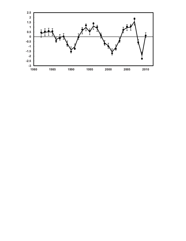
Figure 1: MLE (dots) and posterior mean (solid line) of systematic factor $X_{t}$. Error bars correspond to posterior standard deviation of $X_{t}$.

The MCMC predictions on stressed PD, LGD and EC in comparison with corresponding MLEs are shown in Table 2. MLE for EC is $35\%$ lower than the posterior mean, $24\%$ lower than the posterior median and more than $50\%$ lower than the 0.75 quantile of the posterior for EC. The uncertainty in the posterior of EC is large, CV is about 34.5%; also note a large difference between the 0.75 and the 0.25 quantiles of EC posterior. Underestimation of EC by MLE in comparison with posterior estimates is significant due to large parameter uncertainty and large skeweness in EC posterior. Also, we get the following results for the 0.999 quantile ${Q}^{P}_{0.999}$ of the full predictive loss density for portfolios with different number of borrowers $J$: $Q^{P}_{0.999}=(0.1454,0.1092,0.1026,0.1026)$ for $J=(50,500,5000,\infty)$ respectively. The diversification effect when $J$ increases is evident. In particular, $Q^{P}_{0.999}$ at $J=500$ is about $25\%$ lower than the case at $J=50$; and for $J=5000$ is virtually the same as for the limiting case $J=\infty$. Note that ${Q}^{P}_{0.999}$ at $J=\infty$ is about 50% larger than MLE for EC; and about 15% larger than the posterior mean of $Q^{\infty}_{0.999}({\bm{\Theta}})$. The 15% impact of parameter uncertainty on EC gives indication that $1982-2010$ dataset is long enough for a more or less confident use of the model for capital quantification. Of course, a formal model validation should be performed before final conclusion.

Table 2: MLE and MCMC posterior statistics for PD, LGD and EC.

item	MLE	Mean	Stdev	0.25Q	0.5Q	0.75Q	CV
PD	0.0819	0.103	0.029	0.0825	0.0968	0.116	0.288
LGD	0.803	0.847	0.0562	0.808	0.841	0.880	0.066
EC	0.0657	0.0888	0.031	0.0672	0.0814	0.101	0.345

8 Conclusion

Presented methodology allows joint estimation of the model parameters and latent systematic risk factor in the well known LGD model via Bayesian approach and MCMC method. This approach allows an easy calculation of the full predictive loss density $f_{L_{T+1}}(\cdot|\bf y)$ accounting for parameter uncertainty; then the economic capital can be based on the high quantile of this distribution. Given small datasets typically used to fit the model, the parameter uncertainty is large and the posterior is very different from the normal distribution indicating that Gaussian approximation for parameter uncertainties (typically used under the frequentist maximum likelihood approach assuming large sample limit) is not appropriate.

Due to data limitation, we assumed homogeneous portfolio and thus the results should be treated as illustration. However, the results demonstrate that the extra capital to cover parameter uncertainty can be significant and should not be disregarded by practitioners developing LGD models. The approach can be extended to deal with non-homogeneous portfolios, more than one latent factor and mean reversion in the systematic factor. It should not be difficult to incorporate macroeconomic factors as in [12].

Author address

References

- [1] Basel Committee on Banking Supervision. Guidance on Paragraph 468 of the Framework Document. Bank for International Settlements, Basel, July 2005.
- [2] K. Düllmann and M. Trapp. Systematic risk in recovery rates - an empirical analysis of us corporate credit exposures. Discussion Paper, Series2: Banking and Financial Supervision, pages 1–44, 2004.
- [3] J. Frye. Depressing recoveries. Risk, 13:106–111, 2000.
- [4] M. Gordy. A risk-factor foundation for ratings-based bank capital rules. Finance and Economics Discussion Series 2002-55, Washington: Board of Governors of the Federal Reserve System, 2002.
- [5] X. Luo, P. V. Shevchenko, and J. Donnelly. Addressing impact of truncation and parameter uncertainty on operational risk estimates. The Journal of Operational Risk, 2(4):3–26, 2007.
- [6] Moody’s. Corporate default and recovery rates, 1920-2010. Technical report, February 2011.
- [7] G. W. Peters, P. V. Shevchenko, and M. V. Wüthrich. Dynamic operational risk: modelling dependence and combining different data sources of information. The Journal of Operational Risk, 4(2):69–104, 2009.
- [8] G. W. Peters, P. V. Shevchenko, and M. V. Wüthrich. Model uncertainty in claims reserving within Tweedie’s compound poisson models. ASTIN Bulletin, 39(1):1–33, 2009.
- [9] M. Pykhtin. Unexpected recovery risk. Risk, 16(8):74–78, 2003.
- [10] C. P. Robert. The Bayesian Choice. Springer Verlag, New York, 2001.
- [11] G. O. Roberts and J. S. Rosenthal. Optimal scaling for various Metropolis-Hastings algorithms. Statistical Science, 16:351–367, 2001.
- [12] D. Rösch and H. Scheule. A multifactor approach for systematic default and recovery risk. The Journal of Fixed Income, 15(2):63–75, 2005.
- [13] P. V. Shevchenko. Estimation of operational risk capital charge under parameter uncertainty. The Journal of Operational Risk, 3(1):51–63, 2008.
- [14] P. V. Shevchenko. Modelling Operational Risk Using Bayesian Inference. Springer, Berlin, 2011.
- [15] P. V. Shevchenko and G. Temnov. Modeling operational risk data reported above a time-varying threshold. The Journal of Operational Risk, 4(2):19–42, 2009.