$\alpha_{s}$ from $\tau$ decays revisited

Abstract

Being a determination at low energies, the analysis of hadronic $\tau$ decay data provides a rather precise determination of the strong coupling $\alpha_{s}$ after evolving the result to $M_{Z}$. At such a level of precision, even small non-perturbative effects become relevant for the central value and error. While those effects had been taken into account in the framework of the operator product expansion, contributions going beyond it, so-called duality violations, have previously been neglected. The following investigation fills this gap through a finite-energy sum rule analysis of $\tau$ decay spectra from the OPAL experiment, including duality violations and performing a consistent fit of all appearing QCD parameters. The resulting values for $\alpha_{s}(M_{\tau})$ are $0.307(19)$ in fixed-order perturbation theory and $0.322(26)$ in contour-improved perturbation theory, which translates to the $n_{f}=5$ values $0.1169(25)$ and $0.1187(32)$ at $M_{Z}$, respectively.

1 Introduction

The presented contribution summarises the recent article [1], which laid out a new framework to determine the strong coupling $\alpha_{s}$ from hadronic $\tau$ decays. After the determination of the order $\alpha_{s}^{4}$ coefficient to the QCD Adler function [2], interest in the extraction of $\alpha_{s}$ from $\tau$ decays was revived [2, 3, 4, 5]. However, the results obtained in two approaches to resumming the perturbative series, fixed-order perturbation theory (FOPT) and contour-improved perturbation theory (CIPT), are only barely compatible.

While this issue will be left untouched here, the $\alpha_{s}$ determination from $\tau$ decays also requires numerical inputs for the non-perturbative contributions that arise in the framework of the operator product expansion (OPE), the QCD condensates. Even though the OPE terms are usually included in the analysis, contributions which go beyond it, so-called duality violations (DVs), and which arise due to the presence of resonances on the physical, Minkowskian axis, have so far been neglected. However, for a consistent estimate of the OPE contributions, effects of DVs should be included since typically several spectral integrals of the experimental data with differing weight functions, and possibly at varying energies, are employed, to which the DVs contribute differently. An effort to fill this gap was initiated in the work of ref. [1].

2 Theoretical framework

The central observables for the analysis of hadronic $\tau$ decay are the total decay rate into hadrons,

$$R_{\tau}\,\equiv\,\frac{\Gamma[\tau^{-}\to\nu_{\tau}\,\rm{hadrons}]}{\Gamma[\tau^{-}\to\nu_{\tau}\,e^{-}\,\overline{\nu}_{e}]}\,,$$ (1)

and corresponding differential decay spectra. Experimentally, those spectra can be decomposed into the non-strange vector ($V$) and axial-vector ($A$), as well as the strange components.

The theoretical description is based on the two-point correlation functions

$$\Pi_{V,A}^{\mu\nu}(q)\!\!\! \equiv \!\!\!i\!\int\!{\rm d}^{4}\!x\,e^{iqx}\,\langle 0|T\{J_{V,A}^{\mu}(x)J_{V,A}^{\nu\,\dagger}(0)\}|0\rangle$$

$$= \!\!\!(q^{\mu}q^{\nu}-g^{\mu\nu}q^{2})\,\Pi_{V,A}^{(1)}(q^{2})+q^{\mu}q^{\nu}\Pi_{V,A}^{(0)}(q^{2})\,,$$

where the relevant $V$ and $A$ currents are given by $J_{V}^{\mu}(x)=\overline{u}(x)\gamma^{\mu}d(x)$ and $J_{A}^{\mu}(x)=\overline{u}(x)\gamma^{\mu}\gamma_{5}d(x)$, and the superscripts $(1,0)$ label the spin.

Employing the physical spectral functions $\rho_{V,A}^{(J)}(s)\equiv{\rm Im}\,\Pi_{V,A}^{(J)}(s)/\pi$, the $V$ and $A$ contributions to eq. (1) can be expressed as the $s_{0}=M_{\tau}^{2}$ version of the weighted integral [7]

$$R_{V,A}(s_{0})\!\!\! = \!\!\!12\pi^{2}\,S_{\rm EW}\,|V_{ud}|^{2}\int\limits_{0}^{s_{0}}\frac{{\rm d}s}{s_{0}}\;\Big{(}1-\frac{s}{s_{0}}\Big{)}^{2}\times$$ (3)

$$\Big{[}\,\Big{(}1+2\,\frac{s}{s_{0}}\Big{)}\,\rho_{V,A}^{(1+0)}(s)-2\,\frac{s}{s_{0}}\,\rho_{V,A}^{(0)}(s)\,\Big{]}\,.$$

The scalar/pseudoscalar ($J=0$) terms are suppressed by factors of $m_{u,d}^{2}$, and hence negligible, apart from the pion-pole contribution. Thus, the experimental decay distributions essentially determine $\rho_{V,A}^{(1+0)}(s)$.

Making use of Cauchy’s theorem, the analytic structure of $\Pi_{V,A}^{(1+0)}(s)$ implies that for any analytic weight $w(s)$ the following finite energy sum rule (FESR) is satisfied [8]:

$$\int\limits_{0}^{s_{0}}\!{\rm d}s\,w(s)\,\rho_{V,A}^{(1+0)}(s)\,=\,\frac{i}{2\pi}\!\oint\limits_{|s|=s_{0}}\!{\rm d}s\,w(s)\,\Pi_{V,A}^{(1+0)}(s)\,.$$ (4)

The central idea then is to evaluate the LHS of (4) from experimental data, and the RHS within the theoretical QCD description, thereby allowing to determine fundamental QCD parameters like $\alpha_{s}$.

Conventionally, the theoretical side is calculated in the framework of the operator product expansion. However, the contour integral has to be performed down to the physical, Minkowskian axis, where the OPE breaks down due to the presence of resonances, and quark-hadron duality violations arise. Even though the kinematic weight in (3) has a double zero at $s=s_{0}$, which may suppress DVs, for a general weight $w(s)$ those contributions should be included.

The theoretical 2-point correlators $\Pi_{V,A}^{(1+0)}(s)$ will thus be represented as

$$\Pi_{V,A}^{(1+0)}(s)\,=\,\Pi_{V,A}^{\rm OPE}(s)+\Delta_{V,A}(s)\,,$$ (5)

where the second term corresponds to the DV contribution. Further assuming that it vanishes sufficiently fast at infinity, the required contour integral containing $\Delta_{V,A}(s)$ can be expressed as

$$\frac{i}{2\pi}\!\oint\limits_{|s|=s_{0}}\!{\rm d}s\,w(s)\,\Delta_{V,A}(s)\,=\,-\int\limits_{s_{0}}^{\infty}\!{\rm d}s\,w(s)\,\rho_{V,A}^{\rm DV}(s)\,.$$ (6)

Guided by a model for the light-quark V/A correlators [9], being based on Regge theory and large-$N_{c}$, we employ for $\rho_{V,A}^{\rm DV}(s)$ the Ansatz [10, 11]

$$\rho_{V,A}^{\rm DV}(s)\,=\,\kappa_{V,A}\,{\rm e}^{-\,\gamma_{V,A}s}\sin\left(\alpha_{V,A}+\beta_{V,A}s\right)\,.$$ (7)

Such a model for DVs is also supported by a study of the Coulomb system [12]. Besides the QCD parameters, per channel this adds four additional parameters into the theoretical description, all of which should be extracted through fits to experiment.

3 Numerical analysis

The central strategy to extract all parameters, the strong coupling $\alpha_{s}$, the OPE parameters, as well as DVs, is a simultaneous fit to weighted spectral integrals (moments) of the form (4) with in general different weights $w(s)$ and/or different $s_{0}$, with several criteria restricting the set of sensible choices.

First of all, for simplicity, only weights polynomial in $s$ will be considered. Next, as we intend to extract the parameters for DVs, a weight without pinch-suppression (a zero at $s=s_{0}$) should be included. The simplest choice here is $w(s)=1$. The order of the selected polynomial also determines the dimension up to which OPE terms contribute at leading-order (neglecting logarithmically suppressed effects). For a polynomial of highest order $s^{n}$, operators up to dimension $D=2n+2$ contribute. As very little is known about OPE contributions beyond $D=8$, $w(s)$ will be restricted to at most 3rd order. The kinematical weight of eq. (3) is of this type. Furthermore, below some minimal $s_{0}\approx 1.5\,{\rm GeV}^{2}$, both, the OPE as well as the perturbative expansion become questionable and also the DV model is no longer adequate. Hence only moments down to such a value should be included. Finally, the moments for considered weights/$s_{0}$ combinations are correlated, and for the fits to work these correlations should not become too strong. This is the most delicate point about our analysis.

The required $V$ and $A$ spectral functions have been experimentally determined by the ALEPH [13, 14] and OPAL [15] collaborations at LEP. However, the most recent publicly available ALEPH data [14] do not fully include correlations due to unfolding. Therefore, we chose to perform our analysis on the basis of the OPAL data [15] only.

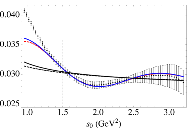
Figure 1: Comparison of experimental and theoretical $w(s)=1$ $V$ moments. FOPT fits are shown in blue (solid) and CIPT fits in red (dashed). The (much flatter) black curves display only the OPE parts of the FOPT (solid) and CIPT (dashed) fit results.

Let us begin by discussing the most basic fit employing only $w(s)=1$ as the weight. In this case, $s_{0}$’s corresponding to the upper endpoints of all experimental bins down to $s_{\rm min}\approx 1.5\,{\rm GeV}^{2}$ can be included if the fit is performed only on the $V$ spectrum, and the fit parameters then only consist of $\alpha_{s}$ and the four $V$-channel DV parameters. The comparison of the moments as computed from the OPAL data and theoretical prediction with fitted parameters is displayed in figure 1. The blue (solid) and red (dashed) lines correspond to FO and CI perturbative results respectively. For comparison the flatter black solid and dashed lines correspond to the same fits omitting DVs, which clearly demonstrates that it is necessary to include them in order to obtain a reasonable fit. The $\alpha_{s}$ values resulting from the fit read

$$\alpha_{s}(M_{\tau})\!\!\! = \!\!\!0.307\pm 0.018\pm 0.004\quad\mbox{(FOPT)}\,,$$ (8)

$$\alpha_{s}(M_{\tau})\!\!\! = \!\!\!0.322\pm 0.025\pm 0.004\quad\mbox{(CIPT)}\,,$$ (9)

where the first error is the fit uncertainty and the second results from a variation of $s_{\rm min}$. The corresponding DV parameters can be found in table 1 of [1]. Similarly to previous $\alpha_{s}$ determinations from $\tau$ decays [2, 3, 4, 5], the FOPT result turns out to be lower than the CIPT value, though due to the additional DV parameters the errors turn out larger and the difference is less significant.

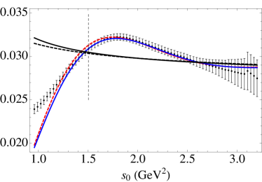
Figure 2: Comparison of experimental and theoretical $w(s)=1$ $A$ moments. FOPT fits are shown in blue (solid) and CIPT fits in red (dashed). The (much flatter) black curves display only the OPE parts of the FOPT (solid) and CIPT (dashed) fit results.

The next level of sophistication is including the axial channel in the fit with $w(s)=1$. This introduces the axial DV parameters as additional fit parameters. It is found, however, that a fit employing the full set of $s_{0}$, corresponding to all right bin endpoints above $s_{\rm min}$, is no longer possible. A stable fit is still obtained, though, if only every third $s_{0}$ is included. The comparison of the vector moments in this case looks very much like figure 1. In figure 2, the corresponding comparison is given for the $A$ moments, with the notation being the same as for figure 1. Again, a fit without DVs would not provide an acceptable description of the data. The resulting values for $\alpha_{s}$ are found to be

$$\alpha_{s}(M_{\tau})\!\!\! = \!\!\!0.308\pm 0.016\pm 0.009\quad\mbox{(FOPT)}\,,$$ (10)

$$\alpha_{s}(M_{\tau})\!\!\! = \!\!\!0.325\pm 0.022\pm 0.011\quad\mbox{(CIPT)}\,,$$ (11)

very similar to the vector only case, but somewhat less stable under variation of $s_{\rm min}$. A full account of all fit parameters is found in table 3 of [1].

Regarding fits including several weight functions, the additional weights $w(x)=1-x^{2}$ with $x\equiv s/s_{0}$ and the kinematical weight $w(x)=(1-x)^{2}(1+2x)$ have been investigated by us in detail. The first one has a single pinch suppression and includes the $D=6$ OPE term while the second is doubly pinched and involves condensates up to $D=8$. As soon as a second weight is added to the fit, even reducing the number of employed $s_{0}$ only leads to very unstable fits, due to the strong correlations. Thus, for these fits we have decided to follow a different route. Here the cross-correlations between different weights are dropped in the fit, but later again included by a linear fluctuation analysis. This again yields results fully compatible with the ones given above, though without a reduction in the error of $\alpha_{s}$.

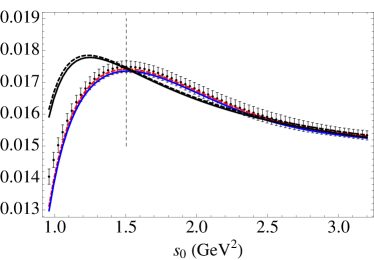
Figure 3: Comparison of experimental and theoretical $w(x)=(1-x)^{2}(1+2x)$ $V$ moments. FOPT fits are shown in blue (solid) and CIPT fits in red (dashed). The black curves display only the OPE parts of the FOPT (solid) and CIPT (dashed) fit results.

As one example figure 3 displays the moment comparison for the kinematical weight. Due to the double pinch suppression, the pure OPE fares much better even down to lower energies. Still, below roughly $s_{0}\approx 2.5\,{\rm GeV}^{2}$ differences to the full fit including DVs are clearly visible. Furthermore, the inclusion of the DVs also influences the values of the fitted condensate parameters. This is exemplified by a more detailed discussion of the $D=6$ condensates and violations of the vacuum-saturation approximation which can be found in section VI.B of ref. [1].

4 Conclusions

Based on ref. [1], a brief summary of the determination of $\alpha_{s}$ from hadronic $\tau$ decays including effects due to duality violations in a consistent fashion has been presented above. The central result will be taken from eqs. (8) and (9), since as far as OPE contribution is concerned, the weight $w=1$ is most clean. Evolving this result to the $Z$ boson mass, one obtains:

$$\alpha_{s}(M_{Z})\!\!\! = \!\!\!0.1169\pm 0.0025\quad\mbox{(FOPT)}\,,$$ (12)

$$\alpha_{s}(M_{Z})\!\!\! = \!\!\!0.1187\pm 0.0032\quad\mbox{(CIPT)}\,.$$ (13)

Our results are somewhat lower than the most frequently quoted previous $\alpha_{s}$ values from $\tau$ decays, but on the other hand the uncertainty is increased in view of the additional degrees of freedom in the fit through the DVs.

The analysis presented in [1] and this contribution was based on the original OPAL data [15], in order to clearly be able to compare to this analysis and single out the effect of including DVs. The corresponding results by OPAL for $\alpha_{s}(M_{Z})$ read $0.1191(16)$ and $0.1219(20)$ for FOPT and CIPT respectively.

As an obvious next step, the analysis should be repeated with an updated data set which includes up-to-date $\tau$ branching fractions and values of other inputs. Such an analysis is currently under way. Then, for comparison, an analysis of the eventually updated ALEPH data would be most helpful, especially as the errors from this data set are expected to be smaller. Finally, in the long run, it is to be hoped that also the B-factories BaBar and Belle will at some point provide the complete $V$ and $A$ spectral functions, since with the available statistics, substantial improvements over the LEP experiments are to be envisaged.

Acknowledgments

We would like to thank Sven Menke for significant help with understanding the OPAL spectral-function data. DB, MJ and SP are supported by CICYTFEDER-FPA2008-01430, SGR2005-00916 and the Spanish Consolider-Ingenio 2010 Program CPAN (CSD2007-00042). SP is also supported by a fellowship from the Programa de Movilidad PR2010-0284. OC is supported in part by MICINN (Spain) under Grant FPA2007-60323, the Spanish Consolider-Ingenio 2010 Program CPAN (CSD2007-00042) and by the DFG cluster of excellence “Origin and Structure of the Universe.” MG and JO are supported in part by the US Department of Energy, and KM is supported by a grant from the Natural Sciences and Engineering Research Council of Canada.

References

- [1] D. R. Boito, O. Cata, M. Golterman, M. Jamin, K. Maltman, J. Osborne, S. Peris, Phys. Rev. D84 (2011) 113006. arXiv:1110.1127.
- [2] P. A. Baikov, K. G. Chetyrkin, J. H. Kühn, Phys. Rev. Lett. 101 (2008) 012002. arXiv:0801.1821.
- [3] M. Davier, S. Descotes-Genon, A. Höcker, B. Malaescu, Z. Zhang, Eur. Phys. J. C56 (2008) 305. arXiv:0803.0979.
- [4] M. Beneke, M. Jamin, JHEP 0809 (2008) 044. arXiv:0806.3156.
- [5] K. Maltman, T. Yavin, Phys. Rev. D78 (2008) 094020. arXiv:0807.0650.
- [6] D. R. Boito, O. Cata, M. Golterman, M. Jamin, K. Maltman, J. Osborne, S. Peris. arXiv:1112.4202.
- [7] E. Braaten, S. Narison, A. Pich, Nucl. Phys. B373 (1992) 581.
- [8] R. Shankar, Phys. Rev. D15 (1977) 755.
- [9] B. Blok, M. A. Shifman, D.-X. Zhang, Phys. Rev. D57 (1998) 2691. arXiv:hep-ph/9709333.
- [10] O. Cata, M. Golterman, S. Peris, JHEP 0508 (2005) 076. arXiv:hep-ph/0506004.
- [11] O. Cata, M. Golterman, S. Peris, Phys. Rev. D77 (2008) 093006. arXiv:0803.0246.
- [12] M. Jamin, JHEP 1109 (2011) 141. arXiv:1103.2718.
- [13] R. Barate, et al., Eur. Phys. J. C4 (1998) 409.
- [14] S. Schael., et al., Phys. Rept. 421 (2005) 191. arXiv:hep-ex/0506072.
- [15] K. Ackerstaff, et al., Eur. Phys. J. C7 (1999) 571. arXiv:hep-ex/9808019.