A series expansion for the time autocorrelation of dynamical variables

Abstract

We present here a general iterative formula which gives a (formal) series expansion for the time autocorrelation of smooth dynamical variables, for all Hamiltonian systems endowed with an invariant measure. We add some criteria, theoretical in nature, which enable one to decide whether the decay of the correlations is exponentially fast or not. One of these criteria is implemented numerically for the case of the Fermi-Pasta-Ulam system, and we find indications which might suggest a sub-exponential decay of the time autocorrelation of a relevant dynamical variable.

1 Introduction

It is well known that one of the most important indicators of the chaotic behaviour of a dynamical system is the rate of decay to zero of the time autocorrelation of dynamical variables. A vast literature exists on this subject, mainly addressed to systems of some special class (for example, Anosov systems, see [1], or systems with few degrees of freedom, such as billiards, see [2]). In this paper we study the decay of correlations in the general frame of the dynamical theory of Hamiltonian systems, with an invariant measure. Such an approach has already provided interesting results, as it allows to obtain results valid in the thermodynamic limit (see [3, 4, 5]).

Here we provide a power series expansion (with respect to time) of the time autocorrelation of a smooth function $f$ (Theorem 2, Section 2). It turns out that the coefficients of such a series are essentially the variances of $L_{H}^{n}f$, where $L_{H}$ is the Poisson bracket operator relative to the Hamiltonian $H$. We then establish a necessary and sufficient condition for its time-decay not to be exponential (Corollary 1, Section 3). We finally give a numerical application to the case of the Fermi-Pasta-Ulam system (FPU). By truncating the series up to order 12, for systems up to 364 degrees of freedom, we approximate the poles of the Laplace transform of the time autocorrelation of a suitably chosen dynamical variable. Some comments are made on the possibility that such approximations give indications for a sub-exponential decay of the autocorrelation.

In Section 2 the relevant notions on time correlation functions are recalled. In the same section we give a theorem which establishes a kind of continuity (with respect to a suitable distance) of time correlations in the $L^{2}$ space of the dynamical variables, and also Theorem 2 for the series expansion.

Section 3 is devoted to a study of some general properties of the series expansion. Here an interesting link with the Stieltjes moment problem is pointed out (see Theorem 3), and a necessary and sufficient criterion for the time-decay of the autocorrelation to be exponential is given as Corollary 1. A closer examination of this problem is given in Appendix A.

Then, the results of some numerical computations on the time autocorrelations of a significant variable in a FPU chain are reported in Section 4. Finally, in Section 5 some comments on the usefulness of the present method are also given. Two more Appendices complete the paper.

2 Time correlations in their “natural” space

We recall here some standard concepts within the measure theoretic approach to dynamical systems. We consider a Hamiltonian system on a phase space $\mathcal{M}$ endowed with a probability measure $\mu$ invariant with respect to the time flow $\phi^{t}$ induced by the Hamiltonian $H$. We also consider the time evolution operator $\hat{U}_{t}$ acting on the space of the square integrable functions from $\mathcal{M}$ to $\mathbb{R}$, i.e., $L^{2}(\mu,\mathcal{M})$. The operator $\hat{U}_{t}$ maps $f$ to $\hat{U}_{t}f=f\circ\phi^{-t}$. It is known after Koopman (see [6]) that $\hat{U}_{t}$ defines a one-parameter group of unitary operators, namely operators preserving the norm $\|\cdot\|$ in $L^{2}(\mu,\mathcal{M})$.

We are interested in the time autocorrelation of a dynamical variable $f\in L^{2}(\mu,\mathcal{M})$, which is defined as

$$\mathbf{C}_{f}(t)\buildrel{\rm def}\over{=}\langle f_{t}\,f\rangle-\langle f\rangle^{2}=\left\langle\left(f_{t}-\langle f\rangle\right)\left(f-\langle f\rangle\right)\right\rangle\ ,$$ (1)

where $f_{t}$ is a shorthand for $\hat{U}_{t}f$, and $\langle\cdot\rangle$ denotes mean value with respect to the probability measure $\mu$.

It will also be useful to consider the time correlation between two dynamical variables $f$ and $g$, defined as

$$\mathbf{C}_{f,g}(t)\buildrel{\rm def}\over{=}\left\langle f_{t}g\right\rangle-\langle f\rangle\langle g\rangle=\left\langle\left(f_{t}-\langle f\rangle\right)\left(g-\langle g\rangle\right)\right\rangle\ .$$

It is well known from probability theory that the concepts of variance and correlation acquire a geometrical meaning if the covariance between two random variables $f$ and $g$ is used as a scalar product. The covariance is defined as

$$\mathrm{cov}(f,g)\buildrel{\rm def}\over{=}\left\langle\left(f-\langle f\rangle\right)\left(g-\langle g\rangle\right)\right\rangle=\mathbf{C}_{f,g}(0)\ ,$$

This choice leads to take as norm of a dynamical variable $f$ its standard deviation $\sigma_{f}$, defined by

$$\sigma^{2}_{f}\buildrel{\rm def}\over{=}\mathrm{cov}(f,f)=\left\|f\right\|^{2}-\left\langle f\right\rangle^{2}=\left\|f-\langle f\rangle\right\|^{2}\ ,$$

$\sigma^{2}_{f}$ being the variance of $f$.

The notion that some relation exists between two random variables $f$ and $g$ is made quantitative through the correlation coefficient $\mathrm{r}(f,g)$ defined as

$$\mathrm{r}(f,g)\buildrel{\rm def}\over{=}\mathrm{cov}(f,g)/\sigma_{f}\sigma_{g}\ .$$

Using the Schwarz inequality it is easily seen in our case that one has $|\mathrm{cov}(f,g)|\leq\sigma_{f}\sigma_{g}$, so that $|\mathrm{r}(f,g)|\leq 1$. Two variables are orthogonal in this metric if they are uncorrelated, i.e., if $\mathrm{r}(f,g)=0$, and collinear if $\mathrm{r}(f,g)=\pm 1$.

We also emphasise that, in view of the above definitions, the time autocorrelation of a function $f$ is nothing but the covariance between $\hat{U}_{t}f$ and $f$. Therefore one immediately has

$$\mathbf{C}_{f}(0)=\sigma^{2}_{f}\quad\mbox{and }\left|\mathbf{C}_{f}(t)\right|\leq\sigma_{f}^{2}\ .$$ (2)

Thus, the variance of a dynamical variable is the natural scale of its time autocorrelation.

We come now to state two useful theorems. The first one points out an interesting property of the time correlation. The mere fact that two dynamical variables are strongly correlated (i.e., sufficiently collinear in the scalar product given by the covariance) entails a similar behaviour of their time autocorrelations. Equivalently, we can say that in the neighbourhood of each dynamical variable $f$, i.e., in the set of all dynamical variables strongly correlated with $f$, the behaviour of the time autocorrelations is determined by that of $\mathbf{C}_{f}(t)$.

Theorem 1

Let $\mu$ be a probability measure on the phase space $\mathcal{M}$, invariant for the flow generated by $H$, and let $f$ and $g$ be dynamical variables belonging to $L^{2}(\mu,\mathcal{M})$ such that one has $|\mathrm{r}(f,g)|\geq 1-{\varepsilon}^{2}/2$ for some ${\varepsilon}>0$. Then there exists a multiple $\tilde{f}=\alpha f$ of $f$, with $\alpha\buildrel{\rm def}\over{=}(\mathrm{sign}(\mathrm{r}(f,g))\sigma_{g}/\sigma_{f})$, such that

$$\bigl{|}\mathbf{C}_{\tilde{f},g}(t)-\mathbf{C}_{\tilde{f}}(t)\bigr{|}\leq{\varepsilon}\sigma_{g}^{2}$$ (3)

and

$$\bigl{|}\mathbf{C}_{g}(t)-\mathbf{C}_{\tilde{f}}(t)\bigr{|}\leq\left({\varepsilon}^{2}+2{\varepsilon}\right)\sigma^{2}_{g}\ .$$ (4)

Proof. Both inequalities come from the remark that

$$\sigma_{g-\tilde{f}}=\sigma^{2}_{g}+\sigma^{2}_{\tilde{f}}-2\mathrm{cov}(\tilde{f},g)=2\sigma^{2}_{g}-2\sigma^{2}_{g}\mathrm{r}(f,g)\leq{\varepsilon}^{2}\sigma^{2}_{g}\ ,$$

which is due to the identities $\sigma_{\tilde{f}}=\sigma_{g}$ and $\mathrm{r}(\tilde{f},g)=\bigl{|}\mathrm{r}(f,g)\bigr{|}$. In fact, (3) hence follows by noting that

$$\bigl{|}\mathbf{C}_{\tilde{f},g}(t)-\mathbf{C}_{\tilde{f}}(t)\bigr{|}=\bigl{|}\mathrm{cov}(\tilde{f}_{t},g)-\mathrm{cov}(\tilde{f}_{t},\tilde{f})\bigr{|}=\bigl{|}\mathrm{cov}(\tilde{f}_{t},g-\tilde{f})\bigr{|}\leq\sigma_{g\phantom{\tilde{f}}}\!\!\sigma_{g-\tilde{f}}\ ,$$

while, in a similar way, (4) comes from the following relations

$$\begin{split}\bigl{|}\mathbf{C}_{g}(t)-\mathbf{C}_{\tilde{f}}(t)\bigr{|}&=\bigl{|}\mathbf{C}_{g-\tilde{f}}(t)+\mathbf{C}_{g,\tilde{f}}(t)+\mathbf{C}_{\tilde{f},g}(t)-2\mathbf{C}_{\tilde{f}}(t)\bigr{|}\\ &\leq\sigma^{2}_{g-\tilde{f}}+2\sigma_{g\phantom{\tilde{f}}}\!\!\sigma_{g-\tilde{f}}\ .\end{split}$$

Here, in the second line, use is made of the previous inequality and of the identity $\mathbf{C}_{g,\tilde{f}}(t)=\mathbf{C}_{\tilde{f},g}(-t)$, due to the invariance of the measure.

Q.E.D.

A central role in this paper will be played by the formal power series expansion of $\mathbf{C}_{f}(t)$ with respect to time, which is given in the following theorem. Use will be made of the definition of the $k$-th order Lie derivative of $f$, for $k\geq 1$, namely $f^{(k)}\buildrel{\rm def}\over{=}[f^{(k-1)},H]$, where $f^{(0)}\buildrel{\rm def}\over{=}f$ and $[\cdot,\cdot]$ denotes the Poisson brackets.

Theorem 2

Let $\mu$ be a probability measure on the phase space $\mathcal{M}$, invariant for the flow generated by $H$, and let $n>0$. Then, for any dynamical variable $f\in L^{2}(\mu,\mathcal{M})$ such that $f^{(k)}\in L^{2}(\mu,\mathcal{M})$ for all $k\leq n$, one has

$$\begin{split}\mathbf{C}_{f}(t)=&\sigma^{2}_{f}+\sum_{k=1}^{n}(-)^{k}\bigl{\|}f^{(k)}\bigr{\|}^{2}\frac{t^{2k}}{(2k)!}\\ &+(-1)^{n+1}\int_{0}^{t}\mathrm{d}t_{1}\ldots\int_{0}^{t_{2n-1}}\mathrm{d}t_{2n}\bigl{\|}f_{t_{2n}}^{(n)}-f^{(n)}\bigr{\|}^{2}\ .\end{split}$$ (5)

Proof. We use the simple chain of identities

$$\|f_{t}-f\|^{2}=2\sigma^{2}_{f}-2\mathbf{C}_{f}(t)=2\|f\|^{2}-2\langle f_{t}\,f\rangle\ ,$$ (6)

which hold true for any invariant measure, and the remark that

$$f_{t}-f=\int_{0}^{t}\hat{U}_{t-s}\dot{f}\mathrm{d}s,$$ (7)

where $\dot{f}=[f,H]$. One can check equations (6) by writing down the square at the l.h.s., while (7) comes from the variation of constants formula applied to $f_{t}-f$.

We go on by writing the l.h.s. of (6) as

$$\|f_{t}-f\|^{2} = \int\mathrm{d}\mu\int_{0}^{t}\mathrm{d}t^{\prime}\int_{0}^{t}\mathrm{d}t^{\prime\prime}\bigl{(}\hat{U}_{t-t^{\prime}}\dot{f}\bigr{)}\bigl{(}\hat{U}_{t-t^{\prime\prime}}\dot{f}\bigr{)}$$ (8)

$$= \int\mathrm{d}\mu\int_{0}^{t}\mathrm{d}t^{\prime}\int_{0}^{t}\mathrm{d}t^{\prime\prime}\bigl{(}\hat{U}_{t^{\prime}-t^{\prime\prime}}\dot{f}\bigr{)}\dot{f}$$

$$= 2\int_{0}^{t}\mathrm{d}t^{\prime}\int_{0}^{t^{\prime}}\mathrm{d}t^{\prime\prime}\left(\bigl{\|}\dot{f}\bigr{\|}^{2}-\frac{1}{2}\bigl{\|}\dot{f}_{t^{\prime\prime}}-\dot{f}\bigr{\|}^{2}\right),$$ (9)

where, in the second line, the invariance of the measure with respect to the time evolution is used, so that the equality proceeds from a simple change of coordinates, and in the last line the same argument is used, as well as relation (6) applied to the variable $\dot{f}$. The order of the integrals can be exchanged if $\|\dot{f}\|$ is finite, because the integral (8) is absolutely convergent in this case, in virtue of Schwarz inequality. In (9) we repeat the same calculation for $\|\dot{f}_{t^{\prime\prime}}-\dot{f}\|^{2}$, using $\dot{f}=[f,H]$. This gives us the relation

$$\left\|f_{t}-f\right\|^{2} = 2\left(\bigl{\|}\dot{f}\bigr{\|}^{2}\frac{t^{2}}{2!}-\bigl{\|}f^{(2)}\bigr{\|}^{2}\frac{t^{4}}{4!}\right)$$

$$+\int_{0}^{t}\mathrm{d}t_{1}\int_{0}^{t_{1}}\mathrm{d}t_{2}\int_{0}^{t_{2}}\mathrm{d}t_{3}\int_{0}^{t_{3}}\mathrm{d}t_{4}\bigl{\|}f^{(2)}_{t_{4}}-f^{(2)}\bigr{\|}^{2}\ ,$$

where $f^{(2)}=[\dot{f},H]$. The same procedure can be iterated up to $k=n$ by recursively defining $f^{(k)}\buildrel{\rm def}\over{=}[f^{(k-1)},H]$, starting with $f^{(0)}\buildrel{\rm def}\over{=}f$, and using the hypothesis that $f^{(k)}\in L^{2}(\mu,\mathcal{M})$. This completes the proof.

Q.E.D.

Remark 1. Theorem 2 suggests that, at least in a formal way, one can express the time autocorrelation of a dynamical variable $f$ as a power series with respect to time

$$\mathbf{C}_{f}(t)=\sigma^{2}_{f}+\sum_{k=1}^{+\infty}(-)^{k}\bigl{\|}f^{(k)}\bigr{\|}^{2}\frac{t^{2k}}{(2k)!}\ .$$ (10)

To simplify the notations, we define

$$c_{0}\buildrel{\rm def}\over{=}\sigma_{f}^{2}\ ,\quad c_{n}\buildrel{\rm def}\over{=}\bigl{\|}f^{(n)}\bigr{\|}^{2}\mbox{ for }n>0\ .$$ (11)

We point out that all these coefficients are positive. We could have got to formula (10) also by expressing $f_{t}$ as a time power series through its Lie derivatives and by integrating $\langle f_{t}\,f\rangle$ by parts, taking into account the observation that the mean value of any function which can be written as $[g,H]$ vanishes, since $\bigl{\langle}[g,H]\bigr{\rangle}=\frac{\mathrm{d}}{\mathrm{d}t}\langle g\rangle$.

Remark 2. We emphasise that the term in the second line in equation (5), i.e., the remainder, turns out to be positive or negative according to $n$ being odd or even, respectively. Therefore, the truncations of series (10) provide upper bounds for the time autocorrelation of $f$ if truncated at an odd $n$, and lower bounds if truncated at an even $n$. Such bounds provide some information on the behaviour of the time autocorrelation of $f$ for finite times. The simplest example is that of the first order truncation, which proved to be very helpful for the study of relaxation times in a Hamiltonian setting (see [3, 4, 5]).

As a final remark, we point out that some a priori restrictions on the norms of the successive derivatives come from the Schwarz inequality (2). Indeed, one has the following Proposition, whose proof is deferred to Appendix B.

Proposition 1

The coefficients $c_{n}$ defined by (11) are such that the polynomials $P_{n}^{l}(y)$, $Q_{n}^{l}(y)$ defined as

$$P_{n}^{l}(y)\buildrel{\rm def}\over{=}2a_{0}^{l}+\sum_{k=1}^{2n}(-)^{k}a_{k}^{l}y^{k}\ ,\quad Q_{n}^{l}(y)\buildrel{\rm def}\over{=}\sum_{k=0}^{2n}(-)^{k}a_{k+1}^{l}y^{k}\ ,$$ (12)

with

$$a_{n}^{l}\buildrel{\rm def}\over{=}c_{n+l}/(2n)!\ ,$$ (13)

are positive semi-definite, for any $n,l\geq 0$.

The statement of Proposition 1 entails some restrictions on the coefficients $c_{n}$, since $P_{n}^{l}(y)$ and $Q_{n}^{l}(y)$ are two-indexed sequences of positive semi-definite polynomials. Unfortunately, such relations can be expressed only in a quite complicated way, through the Jacobi-Borchardt theorem (see, for example, [7]), which gives some relations among the roots of the polynomials, and Newton’s identities on the relations between the coefficients of a polynomial and its roots.

3 Asymptotic behaviour of the correlations

In many cases one is interested in determining whether the time correlation tends to zero as $t\to\infty$ and, if this is the case, which is the law controlling the decay. Indeed, it is commonly stated that if the correlations decay exponentially fast (for a suitable wide class of functions) then the system is chaotic. The decay is linked to the analyticity property of the Fourier transform of the correlations (see for example [8]): in particular it is well known that the Fourier transform is analytic in a strip of width $1/\tau$ if and only if the correlation decays at least as $\exp(-t/\tau)$. We recall that the correlations can always be expressed as the Fourier transform of an even positive measure, the so called “spectral measure”, namely as

$$\mathbf{C}_{f}(t)=\frac{1}{2\pi}\int_{-\infty}^{+\infty}e^{i\omega t}\mathrm{d}\alpha(\omega)\ ,$$ (14)

where $\alpha$ is a positive Borel measure on $\mathbb{R}^{+}$ (see, for example, [11]).

On the other hand, it is not so easy to get information about the spectrum: we devise to get it using the Laplace transform $F(s)$ of the time autocorrelation, namely,

$$F(s)\buildrel{\rm def}\over{=}\int_{0}^{+\infty}e^{-st}\mathbf{C}_{f}(t)\quad\mbox{for }s\in\mathbb{C}\ .$$ (15)

It is well known that the Laplace transform of a function which decays faster than $\exp(-t/\tau)$ is analytic in the half-plane $\operatorname{Re}s>-1/\tau$, so that, again, the control on the decay of correlations in linked to the analyticity properties of $F(s)$, as in the case of the Fourier transform. The great advantage of the latter approach lays in the fact that the Laplace transform of the correlation is essentially the Stieltjes transform of the spectral measure. This is stated as Theorem 3 below.

The point is that, as first shown by Stieltjes (see [9]), if one knows the asymptotic expansion in powers of $1/s$ of a functions $F(s)$ which is the Stieltjes transform of a positive measure, then one can recover $F(s)$ itself through a convergent scheme of continued fractions expansions, defined in terms of the coefficients of the asymptotic expansion. In other words, one can construct a rational approximation

$$F_{n}(s)=\frac{P_{n}(s)}{Q_{n}(s)}\ ,$$

which converges uniformly in $\operatorname{Re}s>0$, as $n\to+\infty$, to $F(s)$. For the case of the time autocorrelation $\mathbf{C}_{f}(t)$, the asymptotic expansion is obtained just by integrating the expansion (10) term by term. In fact, the Laplace transform (15) can be formally written as

$$F(s)=\int_{0}^{+\infty}\left(\sum_{n=0}^{+\infty}(-)^{n}\frac{c_{n}}{(2n)!}t^{2n}\right)e^{-st}\,\mathrm{d}t=\sum_{n=0}^{+\infty}(-)^{n}\frac{c_{n}}{s^{2n+1}}\ .$$ (16)

This expansion would give a convergent expansion, provided one can exchange the sum of the series with the integration over time. This is in general not permissible, in view of the fact that the expansion in power series of time converges (in general) only in a circle of finite radius and not up to infinity. However, it is easy to show that series (16) nevertheless provides the asymptotic expansion of $F(s)$ we are looking for. One has to use formula (5) and check that the remainder grows at most as a power of time.

We are now able to state the main result of this section, namely, the following theorem, together with a relevant corollary on the decay of the correlations.

Theorem 3

Let $\mathbf{C}_{f}(t)$ be analytic in $t$ about the origin and continuous for any $t\in\mathbb{R}$. Then the following statements hold:

1. in the half-plane $\operatorname{Re}s>0$ the Laplace transform $F(s)$ of $\mathbf{C}_{f}(t)$ is analytic and one has

   $$F(s)=\frac{s}{\pi}\int_{0}^{+\infty}\frac{\mathrm{d}\alpha(\omega)}{s^{2}+\omega^{2}}\ ,$$ (17)

   where $\alpha(\omega)$ is the positive Borel measure such that (14) holds;

2. the continued fraction which approximates the asymptotic series (16) converges to $F(s)$ for $\operatorname{Re}s>0$ and the Borel positive measure $\Phi(u)$ defined on $\mathbb{R}^{+}$ by $\Phi(u)\buildrel{\rm def}\over{=}(1/\pi)\alpha(\sqrt{u})$ solves the Stieltjes moment problem for the coefficients $c_{n}$ defined by (11). Moreover, $\alpha(\omega)/\pi$ solves the symmetric Hamburger moment problem with moments $c^{\prime}_{2n}=c_{n}$, $c^{\prime}_{2n+1}=0$.

Corollary 1

$\mathbf{C}_{f}(t)$ decays exponentially fast as $t$ goes to infinity if and only if the coefficients $c_{n}$ are such that $\alpha^{\prime}(\omega)$ exists and $\sqrt{u}\Phi^{\prime}(u)$ is analytic.

Remark 3.We will state our results in terms of the regularity properties of $\alpha$ or $\Phi$ according to convenience. We prefer the study of the properties of $\Phi$, when the convergence properties of Stieltjes continued fraction approximation are needed. Proof of Theorem 3. First of all, we observe that (17) follows by expressing $\mathbf{C}_{f}(t)$ via (14) in the definition (15) of $F(s)$ and exchanging the order of integration. This can be done for any $s$ for which $\operatorname{Re}s>0$, on account of the Tonelli-Fubini theorem for the Stieltjes integral (see [10]), and it is well known that the so defined $F(s)$ is analytic in the same region.

We come now to the proof of statement 2. We notice that the form of series (16) recalls the Stieltjes work [9] on the link between the asymptotic series, their expansion in continued fractions and the Stieltjes transform. In dealing with this subject he met with the moment problem that now bears his name. We recall that, given a sequence of positive numbers $c_{n}$, the Stieltjes moment problem consists in checking whether there exists a measure $\Phi$ on $\mathbb{R}^{+}$ such that

$$\int_{0}^{+\infty}u^{n}\mathrm{d}\Phi(u)=c_{n}\ .$$ (18)

The solution exists if and only if

$$\det(\Delta_{n})\geq 0\quad\mbox{and}\quad\det(\tilde{\Delta}_{n})\geq 0\quad\forall n\ ,$$ (19)

where the matrices $\Delta_{n}$, $\tilde{\Delta}_{n}$ are defined by

$$\Delta_{n}\!\buildrel{\rm def}\over{=}\!\left[\!\begin{array}[]{cccc}c_{0}&c_{1}&\cdots&c_{n}\\ c_{1}&c_{2}&\cdots&c_{n+1}\\ \vdots&\vdots&\ddots&\vdots\\ c_{n}&c_{n+1}&\cdots&c_{2n}\end{array}\!\right]\ ,\ \tilde{\Delta}_{n}\!\buildrel{\rm def}\over{=}\!\left[\!\begin{array}[]{cccc}c_{1}&c_{2}&\cdots&c_{n+1}\\ c_{2}&c_{3}&\cdots&c_{n+2}\\ \vdots&\vdots&\ddots&\vdots\\ c_{n+1}&c_{n+2}&\cdots&c_{2n+1}\end{array}\!\right]\ ,$$ (20)

and if the equality in (19) is obtained for $\Delta_{k}$, then it is obtained for $\Delta_{n}$, with $n\geq k$ and for $\tilde{\Delta}_{n}$, with $n\geq k-1$. Furthermore, the solution is unique if there exists $D>0$ such that

$$c_{n}\leq D^{n}(2n)!\ ,$$ (21)

holds (for a proof with more recent methods, see [12]). We point out that, in our case, since $C_{f}(t)$ is analytic about the origin, there should exist $D>0$ such that the previous condition is satisfied, in view of the Cauchy-Hadamard criterion.

Coming back to our problem, we collect the results of paper [9] of interest to us in the following statement: if the function $F(s)$ admits the representation (17), then the continued fraction which approximates the asymptotic expansion (16) converges to $F(s)$ for $\operatorname{Re}s>0$; moreover, the Stieltjes moment problem for the sequence $c_{n}$ is soluble.

The previous statement is proved this way. In equation (17) we put $z\buildrel{\rm def}\over{=}s^{2}$, $u\buildrel{\rm def}\over{=}\omega^{2}$, $\Phi(u)\buildrel{\rm def}\over{=}\alpha(\sqrt{u})$. Then we have the formal chain of equalities

$$s\int_{0}^{+\infty}\frac{\mathrm{d}\Phi(u)}{z+u}=F(s)=s\left(\frac{c_{0}}{z}-\frac{c_{1}}{z^{2}}+\frac{c_{2}}{z^{3}}+\ldots\right)\ ,$$ (22)

where again $\Phi$ is a Borel positive measure on $\mathbb{R}^{+}$. Stieltjes showed that the continued fraction which approximates the term in brackets at the r.h.s. converges to the integral at the l.h.s, and that the Stieltjes moment problem for the sequence $c_{n}$ has a solution for the measure $\Phi$. Then it is straightforward to check that $\alpha/\pi$ solves the associated symmetric Hamburger moment problem, which means that

$$\frac{1}{\pi}\int_{-\infty}^{+\infty}\omega^{2n}\mathrm{d}\alpha(\omega)=c_{n}\ ,\quad\frac{1}{\pi}\int_{-\infty}^{+\infty}\omega^{2n+1}\mathrm{d}\alpha(\omega)=0\ .$$

Q.E.D.

Remark 4. Notice that we have incidentally shown that the coefficients $c_{n}$ are such that conditions (19) are satisfied at any order. This restriction on the values of the coefficients, together with the analogous ones imposed by the application of the previous theorem to the dynamical variables $f^{(n)}$, for all $n$, already contains the restriction given by Proposition 1. However, we point out that Proposition 1 holds up to a given order even if the existence of $f^{(n)}$ beyond such an order is not guaranteed.

In view of Corollary 1, the question of the asymptotic behaviour of the time autocorrelations can be restated as a regularity problem for the measure $\Phi$, which solves Stieltjes moment problem for the $c_{n}$, or, equivalently, for $\alpha$ which solves the associated Hamburger moment problem. An answer to this question can be given only if the whole sequence of moments $c_{n}$ is known. However, it is also of interest to understand which is the qualitative difference between the approximation (at a given order) of an analytic measure and that of a measure with at least a singular point. We try here to give an answer to the latter question, deferring to Appendix A the discussion of which is the link between the behaviour of the moments and the regularity of the solution (see Proposition 2, 3, 4 therein).

We have already pointed out that a rational approximation $F_{2n}(s)$ of the Laplace transform $F(s)$ can be constructed from (22) by standard methods (see Chapter 2 of Stieltjes memoir [9]), which give

$$F_{2n}(s)=s\frac{P_{2n}(s)}{Q_{2n}(s)}=s\sum_{k=0}^{n}\frac{\rho_{k}}{s^{2}+\omega^{2}_{k}}\ .$$

Such a function, in turn, can be rewritten as the following Stieltjes integral

$$F_{2n}(s)=s\int_{0}^{+\infty}\frac{\mathrm{d}\alpha_{n}(u)}{s^{2}+u}\ ,$$

in which the measure $\alpha_{n}$ is piecewise constant and has a jump $\rho_{k}$ at the points $u=\omega^{2}_{k}$. Therefore, in order that the limiting measure $\alpha=\lim\alpha_{n}$ be continuous, it is necessary that, as the approximation order grows, the poles become dense and their residues tend to zero. As a consequence, we will take as a qualitative indication of a sub-exponential decay the property that the rational approximations have at least a pole which remains isolated, with a stable residue, as the order grows.

4 Numerical study of the FPU chain

Checking whether the spectral measure is analytic, or even whether the criterion of Proposition 2 of Appendix A is satisfied for a concrete problem is a major task, because it requires information on an infinite number of coefficients. Thus, as a first attempt to implement the ideas of Section 3, we computed numerically some coefficients $c_{n}$ for a model which is widely studied in the literature and is of great relevance for the foundations of statistical mechanics, namely the Fermi-Pasta-Ulam model (FPU, see [14]). It describes a one-dimensional chain of $N+1$ particles interacting through nonlinear springs. The Hamiltonian of such a system, after a suitable rescaling, can be written as

$$H=\sum_{j=0}^{N}\frac{p_{j}^{2}}{2}+\sum_{j=0}^{N-1}\left[\frac{\left(q_{j}-q_{j+1}\right)^{2}}{2}+\frac{\alpha\left(q_{j}-q_{j+1}\right)^{3}}{3}+\frac{\beta\left(q_{j}-q_{j+1}\right)^{4}}{4}\right]\ ,$$

where $p=(p_{0},\ldots,p_{N})$ and $q=(q_{0},\ldots,q_{N})$ are canonically conjugated variables, while $\alpha$ and $\beta$ are parameters that control the size of the nonlinearity. We choose as invariant probability measure the Gibbs one, i.e., $\mathrm{d}\mu(p,q)\buildrel{\rm def}\over{=}Z^{-1}(T)\exp(-H(p,q)/T)\mathrm{d}p\,\mathrm{d}q$, where $Z(T)$ is the partition function and $T>0$ the temperature, and for the purpose of speeding up the numerical evaluation of the integrals involving the measure, we consider here a chain with one end point fixed and the other one free, i.e, we impose only the boundary condition $q_{0}=0$, $p_{0}=0$ (see footnote 4 below). We note however that a few computations made on the model in which both end-points are fixed have shown no significant difference. Concerning the parameters, we consider the often studied case in which $\alpha=\beta=1/4$. The relevant fact is that as $T$ approaches 0 the contribution due to the nonlinear terms becomes statistically negligible.

It is well known that if the nonlinear terms are neglected then the Hamiltonian is integrable, admitting $N$ normal modes of oscillation, and that the motion is quasi periodic so that, for every $k=0,\ldots,N-1$, the energy $E_{k}$ of the $k$-th mode is a constant of motion (and thus, as obvious, the time autocorrelation of such a dynamical variable is constant). Our aim is to investigate what happens when the nonlinearity is introduced as a perturbation, namely, for $T$ positive but close to 0. We are particularly interested in the exchange of energy among the normal modes. To this end, a good choice could be to consider the fraction of energy localized on the low frequency modes, defined, for example, as

$$\mathcal{E}=\frac{1}{N}\sum_{k=0}^{N/2}E_{k}\ ,$$

since its time variation is a convenient indicator of the flow of energy from low to high frequency modes, and vice versa. As a numerical tool we want to compute numerically the coefficients of the series (10) for this function, since, in view of Theorem 3, they give indications on the asymptotic behaviour of the autocorrelation.

As a matter of fact, we notice that the function $\mathcal{E}$ may not represent the best choice. For, such a function is strongly correlated with the Hamiltonian, so that, in virtue of Theorem 1, its autocorrelation remains close to that of the Hamiltonian, thus remaining far from zero. So, we rather took a suitable modification of $\mathcal{E}$, namely, the projection of $\mathcal{E}$, via the Gram-Schmidt orthogonalization process, on the space of the dynamical variables uncorrelated with $H$. Thus we consider the dynamical variable $\tilde{\mathcal{E}}\buildrel{\rm def}\over{=}\mathcal{E}-\mathrm{cov}(\mathcal{E},H)H/\sigma^{2}_{H}$.

Our calculation proceeds as follows. We extract a sample in phase space according to the Gibbs measure and we estimate the $L^{2}$-norm $\|\tilde{\mathcal{E}}^{(n)}\|^{2}$ of the functions $\tilde{\mathcal{E}}^{(n)}=[\tilde{\mathcal{E}}^{(n-1)},H]$ generated by $\tilde{\mathcal{E}}^{(0)}=\tilde{\mathcal{E}}$ taking the mean value on our sample. For this purpose, we observe that $\tilde{\mathcal{E}}^{(n)}$ is a certain function of $p$ and $q$, which can be expressed via Faà di Bruno’s formula for the derivatives of any order of a composed function. This formula requires the computation of some combinatorial coefficients, which needs a smart implementation in order to reduce the computation time. We report in Appendix C the scheme we have followed.

In order to study the Laplace transform of the time autocorrelation of $\tilde{\mathcal{E}}$, following the procedure of Stieltjes, we approximate it up to order $n$ with rational functions, and look for the poles of such an approximating function in the complex plane (see chapter 2 of the memoir [9]). Our aim is to compare the behaviour of the time autocorrelation of $\tilde{\mathcal{E}}$ with some functions which behave in a somehow known way, by comparing the poles of the corresponding rational approximations of the Laplace transforms. The first comparison function is the time autocorrelation of a variable which should lose correlation in a very short time, i.e., (the orthogonal projection of) the kinetic energy $\tilde{K}$ of the first half of the chain’s particles. The second one will be a given function of time which has an exponential decay (see below for its actual form).

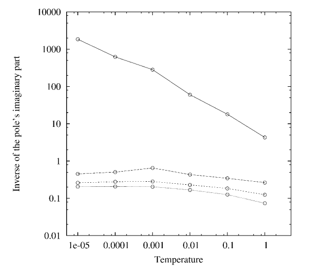
Figure 1: Inverse of the imaginary part of the four poles of the Laplace transform of the time autocorrelation of $\tilde{\mathcal{E}}$ versus temperature, in logarithmic scale. Here the number of particles is $N=40$.

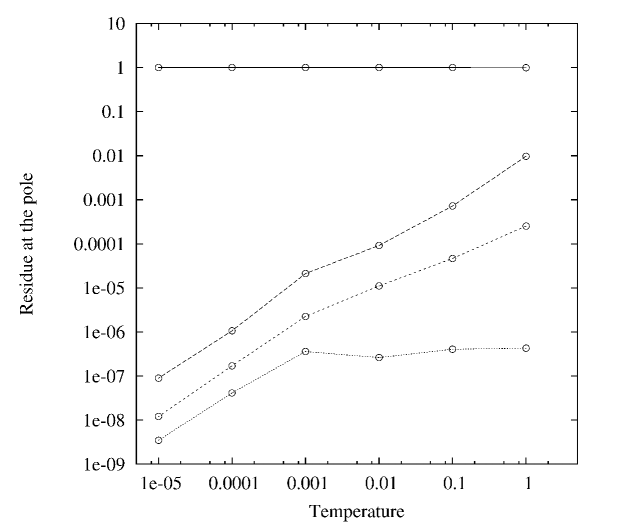
Figure 2: Residues at the four poles, whose imaginary parts are reported in fig. 1 versus temperature, in logarithmic scale. Here the number of particles is $N=40$.

Let us describe the results in some detail. We know that the rational approximation of the Laplace transform at order $2n$ will have $2n$ complex conjugated poles, $s_{k}=i\omega_{k}$, $\bar{s}_{k}=-i\omega_{k}$ say. The inverses of the $\omega$’s so found for the time autocorrelation of $\tilde{\mathcal{E}}$ are plotted in fig. 1 versus temperature $T$. The pole that shows up at order 1 produces the upper curve in the figure. It corresponds to oscillation of a quite large period, growing as $1/T^{1/2}$ as $T$ decreases to zero. The actual value changes a little when the approximation increases, keeping however the same order of magnitude. The plotted data correspond to the approximation order $n=4$. We have also noted that the values found do not significantly change with the number $N$ of particles, for $N$ up to 364. The frequencies represented by the lower curves show up at successive orders $n=2,3,4$, respectively, and correspond to oscillations of a short period, which, at variance with the first period, are of the order of magnitude of the typical periods of the normal modes. They appear to remain almost constant with $T$.

A further information is provided by the residues of the poles, which represent the amplitudes of the oscillations. The quantities for the four poles of fig. 1 are reported in fig. 2, after a normalization defined by setting the sum of the residues equal to one. The remarkable fact is that the amplitude corresponding to the longest period is the largest one. Even for $T=1$ the amplitudes of the shorter periods do not exceed one percent of the total.

It is now of interest to look at the corresponding graphs (fig. LABEL:fig3-LABEL:fig4) for the time autocorrelation of the kinetic energy of half of the chain, $\tilde{K}$. As expected, the time-scales involved are much shorter, as is seen by inspection of fig. LABEL:fig3. In any case, an indication of a bigger chaoticity is given by the fact that all the residues are of the same order of magnitude and are closer to each other, as can be seen in fig. LABEL:fig4. This means that in the spectrum of the time autocorrelation of $\tilde{K}$ at least three frequencies are excited, at variance with the spectrum of $\tilde{\mathcal{E}}$, for which just a frequency is actually excited.

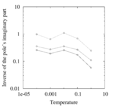
(a)

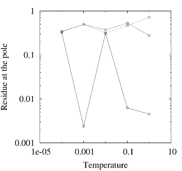
(b)

Figure 3: Location and residues of the first three poles of the Laplace transform of the time autocorrelation of kinetic energy $\tilde{K}$ versus temperature, in logarithmic scale. Here the number of particles is $N=40$.

Then, we compare the behaviour of $\mathbf{C}_{\tilde{\mathcal{E}}}(t)$ with that of $g(t)\buildrel{\rm def}\over{=}\cosh^{-1}(bt)$, where $b>0$, in order to look for possible differences with respect to an exponential decay. Here the constant $b$ is so chosen that the approximation of the Laplace transform of such a function at order $n=1$ has a pole at the same place as the Laplace transform of $\mathbf{C}_{\tilde{\mathcal{E}}}(t)$, for a fixed temperature $T$ (as we have seen, $b\sim 1/T^{1/2}$). In fig. 4 the poles and the corresponding residues of the Laplace transforms of $\cosh^{-1}(bt)$ and $\mathbf{C}_{\tilde{\mathcal{E}}}(t)$ are plotted at the successive orders of approximation $n=3,4$.

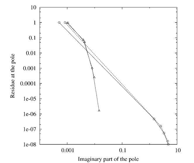
Figure 4: Residues of the poles of the Laplace transforms of $\mathbf{C}_{\tilde{\mathcal{E}}}(t)$ and of $g(t)$ versus their imaginary parts, in logarithmic scale. The circles refer to $\mathbf{C}_{\tilde{\mathcal{E}}}(t)$ and the triangles to $g(t)$, while the dashed lines indicate that the order of approximation is 3, and the continuous lines indicate order 4. Here the number of particles is $N=40$ and $T=10^{-5}$

In both cases a pole of order $10^{-3}$ has the largest residue, but it is apparent that, while for $g(t)$ the other poles are close to that one, in the case of $\mathbf{C}_{\tilde{\mathcal{E}}}(t)$ there seems to remain a jump between the first pole and the others. This fact is in agreement with the remark, already made by Stieltjes, that the poles of the Laplace transform of $g(t)$ become dense on the imaginary axis and corresponds with the fact that the spectral measure is in this case analytic. On the other hand, the same fact seems to suggest a qualitatively different behaviour of $\mathbf{C}_{\tilde{\mathcal{E}}}(t)$, and in particular that $\alpha(\omega)$ is not analytic in this case, so that the decay of the time autocorrelation of $\tilde{\mathcal{E}}$ is not exponential.

As a final remark, we add a few considerations concerning the actual difficulty occurring in the calculations. In view of Theorem 3, all poles lie on the imaginary axis and all the determinants (20) are positive. So, we are certain that the outcome of our computation ceases to be reliable at the order at which we encounter a negative determinant. Since the coefficients are determined via a Monte Carlo approximation of an integral, they are subject to a numerical error. The difficulty is that increasing the order requires also a corresponding increase of the precision, and so a longer and longer calculation. This makes the whole procedure unpractical even at not too high orders, and for this reason we performed most calculations up to order 8 only, thus finding 4 frequencies.

5 Conclusions

We have shown that there is a convergent algorithm which, in principle, could be implemented to get the Laplace transform of the time autocorrelation of a dynamical variable, and so to get conclusions about the rate of its decay as $t\to\infty$. In our opinion, the most relevant aspect is the connection we found between the spectral measure and the solution of the Stieltjes moment problem, which implies a relation between the smoothness property of the measure and the fulfilment of an infinite set of constraints (see, as an example, Proposition 3 in Appendix A). This leads us to the question, whether smooth measures are in some sense exceptional, namely, to ask whether these constraints can still be satisfied when small changes in the moments are performed (i.e., by generic small perturbations of the Hamiltonian flow).

Implementing such an algorithm on a computer raises major difficulties with respect to both the computational time and the reliability of the results. As a matter of fact, the main problem is connected with the calculation of large determinants. However, we tried to apply the method to two functions of interest fro the FPU problem, namely, the energy of a packet of low frequency modes and the kinetic energy of half of a FPU chain. For the first function, our results seem to support the conjecture that the time autocorrelations exhibit a sub-exponential decay, while no definite conclusions can be drawn for the second quantity. We remark that this is a known characteristic for chains of FPU type, namely that quantities related to the particles typically exhibit a behaviour coherent with the predictions of Statistical Mechanics, while this often does not happen with quantities related to the modes. On the other hand, we should emphasize that the existence of functions with a slow decay of the autocorrelations is in itself an obstacle for the ergodic behaviour of a dynamical system. For similar results, see, e.g., [16].

Appendix A Conditions on the regularity of the measure which solves the moment problem

The problem of determining a necessary and sufficient condition in order that the solution of an Hamburger moment problem admit a bounded positive derivative has been solved by KHz and Krein (see [17]). Unfortunately, their criterion cannot be applied to study the derivative itself. Thus, we report the criterion of Akhiezer and Krein for checking the existence of a derivative for the Hamburger moment problem for the measure $\alpha$, then we give an alternative procedure for studying the derivatives of $\sqrt{u}\Phi^{\prime}(u)$, at least in the case in which the time autocorrelation is analytic on the whole real axis. We convert the problem into an Hausdorff moment problem (i.e., a moment problem on a finite interval), in order to get condition on the regularity of the successive derivatives.

To state the result of [17] of interest to us, let us introduce the definition of a non-negative definite sequence of moments $c_{n}$, by requiring that

$$\sum_{i,j=1}^{n}c_{i+j}X_{i}\bar{X}_{j}\geq 0\ ,$$

for any $n$ and any sequence $(X_{1},\ldots,X_{n})$ of complex numbers. Then one has

Proposition 2

In order that $\alpha^{\prime}(\omega)$ exist and be bounded, it is necessary and sufficient that there exist $L>0$ such that the sequence $t_{0}(L),t_{1}(L),\ldots$ defined by

$$t_{k}(L)=\frac{1}{(k+1)!L^{k+1}}\left|\begin{array}[]{cccccc}c^{\prime}_{0}&-L&0&\cdots&0&0\\ 2c^{\prime}_{1}&c^{\prime}_{0}&-2L&\cdots&0&0\\ \vdots&\vdots&\vdots&\ddots&\vdots&\vdots\\ kc^{\prime}_{k-1}&(k-1)c^{\prime}_{k-2}&(k-2)c^{\prime}_{k-3}&\ldots&c^{\prime}_{0}&-kL\\ (k+1)c^{\prime}_{k}&kc^{\prime}_{k-1}&(k-1)c_{k-2}&\ldots&2c^{\prime}_{1}&c^{\prime}_{0}\\ \end{array}\right|\ ,$$

is non-negative definite.

For the study of the successive derivatives, we observe that in paper [13] Hausdorff found a solution method for the moment problem on the interval $[0,1]$, which also allows to give a criterion to check whether, at any order, the derivatives of the measure exist and are bounded. Such results can be also applied to our problem if the time autocorrelation is analytic on the whole real axis, because, through an analytic change of variable, one can map $[0,1]$ on $\mathbb{R}^{+}$ and obtain the next Proposition 3, which provides necessary and sufficient conditions in order that the $n$-th derivative of $\sqrt{u}\Phi^{\prime}(u)$ exist and be bounded. For its statement, we need to define the auxiliary moments $\mu_{k}$ and $\tilde{\mu}_{k}$: we need to preliminarily define

$$\mathfrak{F}(z)\buildrel{\rm def}\over{=}\int_{0}^{+\infty}\frac{\mathrm{d}\Phi(u)}{z+u}\ ,$$

then we set

$$\begin{split}\mu_{0}\buildrel{\rm def}\over{=}c_{0}\,\quad\mu_{k}\buildrel{\rm def}\over{=}c_{0}-\frac{1}{(k-1)!}\frac{\mathrm{d}^{k-1}}{\mathrm{d}^{k-1}z}\left(z^{k}\mathfrak{F}(z)\right)_{z=1}\ ,\mbox{ for }k>0\ ,\\ \tilde{\mu}_{k}\buildrel{\rm def}\over{=}\sum_{n=0}^{\infty}\binom{k+1/2}{n}\sum_{l=0}^{n}\binom{n}{l}(-)^{n-l}2^{l-k-1/2}\mu_{l}\ .\end{split}$$ (23)

These quantities are well defined, since it is known that $\mathfrak{F}(z)$ is analytic in $z=1$ and the binomial expansion converges. Then, we define the quantities

$$\begin{split}\lambda_{p,m}^{0}\buildrel{\rm def}\over{=}\binom{p}{m}\sum_{k=0}^{p-m}(-1)^{k}\binom{p-m}{k}\tilde{\mu}_{k}\ ,\quad\mbox{for }0\leq m\leq p\ ;\\ \lambda_{p,m}^{k}\buildrel{\rm def}\over{=}(p+1)\left(\lambda_{p,m}^{k-1}-\lambda_{p,m-1}^{k-1}\right)\ ,\quad\mbox{for }k>0,k\leq m\leq p-k\ ,\end{split}$$ (24)

and state the following

Proposition 3

Let $\mathbf{C}_{f}(t)$ be an analytic function of $t$, for $t\in\mathbb{R}$, and let $\Phi$ be the measure which solves the related Stieltjes moment problem. A bounded derivative of order $n$ of $\sqrt{u}\Phi^{\prime}(u)$ exists if and only there exist $L_{k}>0$ such that, for any $p>0$, $0\leq k<n$ and $k\leq m\leq p-k$, one has

$$(p+1)\left|\lambda_{p,m}^{k}\right|\leq L_{k}\ .$$ (25)

Proof. The proof is performed through the Euler transformation $w\buildrel{\rm def}\over{=}\frac{u}{u+1}$. This enables one to define the positive Borel measure $\Psi(w)$ on $[0,1]$, by $\Psi(w)\buildrel{\rm def}\over{=}\Phi(w/(1-w))$. The relation between the moments of $\Psi$ on the interval $[0,1]$ and the moments $c_{n}$ of $\Phi$ can be obtained by the following chain of equalities, for $k>0$,

$$\int_{0}^{1}w^{k}\mathrm{d}\Psi(w)=\int_{0}^{+\infty}\frac{u^{k}}{(u+1)^{k}}\mathrm{d}\Phi(u)=\sum_{l=0}^{k}(-)^{k}\binom{k}{l}\int_{0}^{+\infty}\frac{\mathrm{d}\Phi(u)}{(u+1)^{l}}\ ,$$ (26)

as can be seen by expanding $u^{k}=(u+1-u)^{k}$ via the binomial formula. It is easy to see that this implies that the coefficients $\mu_{k}$ defined by (23) are the moments of $\Psi$.

In order to study the derivatives of $\alpha^{\prime}(\omega)=2\sqrt{u}\Phi^{\prime}(u)$, we pass to the the moments given by the distribution function $\sqrt{w}\Psi^{\prime}(w)$. This function exists if $C_{f}(t)$ is analytic on the whole real axis, because in such a case its spectral measure $\alpha(\omega)$ tends exponentially fast towards its limit for $\omega\to\infty$ and, in consequence, $\Psi(w)$ tends towards the same limit as $w\to 1$ at least as fast as $e^{-\kappa/\sqrt{1-w}}$. Moreover, $\sqrt{w}\Psi^{\prime}(w)$ admits a bounded derivative of order $n$ if and only if $\sqrt{u}\Phi^{\prime}(u)$ does. We need, thus, to find the moments of $\sqrt{w}\Psi^{\prime}(w)$, which are given by

$$\int_{0}^{1}w^{k+1/2}\Phi^{\prime}(w)\mathrm{d}w=\int_{0}^{1}\sum_{n=0}^{\infty}\binom{k+1/2}{n}2^{k+1/2-n}\left(w-\frac{1}{2}\right)^{n}\Phi^{\prime}(w)\mathrm{d}w\ ,$$

in view of the binomial expansion of $\sqrt{1/2+(w-1/2)}$. Since this expansion converges uniformly for $w\in[0,1]$, one can exchange the order of summation and integration and prove that these moments are indeed the $\tilde{\mu}_{k}$ defined by (23).

As Hausdorff proved, in order that the moment problem for the sequence $\tilde{\mu}_{k}$ have a solution $\psi_{0}$ on $[0,1]$, which is almost everywhere differentiable with a limited derivative (in our case, it is $\psi_{1}(w)=\sqrt{w}\Psi^{\prime}(w)$), it is necessary and sufficient that $(p+1)|\lambda^{0}_{p,m}|$ be bounded, where $\lambda^{0}_{p,m}$ are defined by equation (24). This corresponds to

$$\lambda^{0}_{p,m}=\binom{p}{m}\int_{0}^{1}w^{m}(1-w)^{p-m}\mathrm{d}\psi_{0}(w)\ .$$

Then, one considers the Hausdorff moment problem in which the measure (not necessarily positive) is $\psi_{1}$, and expresses its moments $\tilde{\mu}^{1}_{k}$ through the original moments $\tilde{\mu}_{k}$, by integrating by parts. So one obtains that the coefficients $\lambda_{p,m}^{1}$ defined by (24) play for $\psi_{1}$ the same role which the $\lambda_{p,m}^{0}$ play for $\psi_{0}$, because, for $1\leq m\leq p-1$,

$$\lambda^{1}_{p,m}=(p+1)(\lambda^{0}_{p,m}-\lambda^{0}_{p,m-1})=\binom{p+1}{m}\int_{0}^{1}w^{m}(1-w)^{p+1-m}\mathrm{d}\psi_{0}(w)\ .$$

Thus, one can express the condition that $\psi_{1}$ admits a limited derivative by asking that $(p+1)|\lambda^{1}_{p,m}|$ have an upper bound. The proof is then concluded by iterating this way of proceeding.

Q.E.D.

Finally, we add the following Proposition, which can be proved by the easy remark that a power series with positive coefficients, which has a radius of convergence $\rho$, has a singularity for $z=\rho$ (this is known as Vivanti’s theorem).

Proposition 4

In order that the decay of the time autocorrelation of the dynamical variable $f$ be not exponentially fast it is sufficient that there exists $\rho>0$ such that $\limsup_{n\to+\infty}\sqrt[n]{c_{n}}\leq\rho$ .

Remark 5. The condition of Proposition 4 requires only to have an upper bound on the $c_{n}$, whereas those of Propositions 2-3 ask for a more detailed knowledge on the coefficients $c_{n}$. We believe that the first one is seldom fulfilled (an example in which it is fulfilled is that of a harmonic oscillator). For, the $n$-th derivative of a function usually grows as $n!$, so that

$$\limsup_{n\to+\infty}\sqrt[n]{c_{n}}=+\infty\ .$$

The other requirements enables us to deal with a larger class of variables, but, as just said, it has the drawback of needing a very detailed knowledge of all coefficients.

Appendix B Proof of Proposition 1

Consider the series (5), and recall that the remainder has a definite sign. Due to the inequalities (2) we readily get the bounds

$$a^{0}_{0}+\sum_{k=1}^{2n}(-)^{k}a^{0}_{k}t^{2k}\geq-a^{0}_{0}\quad\mbox{and}\quad a^{0}_{0}+\sum_{k=1}^{2n+1}(-)^{k}a^{0}_{k}t^{2k}\leq a^{0}_{0}\ ,\quad\forall t\in\mathbb{R}\ ,$$

which hold true because the remainder is negative in the first case and positive in the second one. Setting $y\buildrel{\rm def}\over{=}t^{2}$, we get the inequalities

$$P_{n}(y) \buildrel{\rm def}\over{=} 2a^{0}_{0}+\sum_{k=1}^{2n}(-)^{k}a^{0}_{k}y^{k}\geq 0\ ,$$ (27)

$$Q_{n}(y) \buildrel{\rm def}\over{=} \sum_{k=0}^{2n}(-)^{k}a^{0}_{k+1}y^{k}\geq 0\ ,$$ (28)

i.e., the polynomials $P_{n}(y)$ and $Q_{n}(y)$ are positive semi-definite for $y\geq 0$. Look now for the real roots of the equations $P_{n}(y)=-{\varepsilon}$ and $Q_{n}(y)=-{\varepsilon}$, with $0<{\varepsilon}<{\rm min}\{a_{0},a_{1}\}$. Since $P_{n}(y)$ and $Q_{n}(y)$ are polynomials of degree $2n$ in which $2n$ changes of sign occur, Descartes’ rule of signs implies that such roots, if they exist, must be positive. Thus $P_{n}$ and $Q_{n}$ are positive semi-definite on the whole real axis, i.e., the inequalities (27) hold true for all $y\in\mathbb{R}$.

Consider now the dynamical variable $f^{(l)}$, calculated by recursive application of the Poisson bracket with $H$. By a straightforward application of Theorem 2 we get that the coefficients of $f^{l}$ are precisely $a_{n}^{l}$ as defined in (13). Since the argument above applies to any dynamical variable, then we get that the corresponding polynomials $P_{n}^{l}(y)$ and $Q_{n}^{l}(y)$ are positive semi-definite, too, as claimed.

Appendix C Computation of the coefficients needed for the Faà di Bruno formula

Let us recall the Faà di Bruno’s formula (see [18]). Let a function $f\bigl{(}g(x)\bigr{)}$ be given, where $f$ and $g$ possess a sufficient number of derivatives. Then one has

$$\frac{\mathrm{d}^{n}}{\mathrm{d}x^{n}}f\bigl{(}g(x)\bigr{)}=\sum\frac{n!}{k_{1}!\,k_{2}!\,\cdots\,k_{n}!}\cdot f^{(k_{1}+\cdots+k_{n})}\bigl{(}g(x)\bigr{)}\cdot\prod_{j=1}^{n}\left(\frac{g^{(j)}(x)}{j!}\right)^{k_{j}}\ ,$$

where the sum is over all $n$-tuples of nonnegative integers $(k_{1},\ldots,k_{n})$ satisfying the constraint

$$1\cdot k_{1}+2\cdot k_{2}+3\cdot k_{3}+\cdots+n\cdot k_{n}=n\ .$$

In our case, we apply twice the formula, the first time to find the successive derivatives of the canonical coordinates $q$ and $p=\dot{q}$ with respect to time, the second one to find the derivatives of $\tilde{\mathcal{E}}(p,q)$ and $\tilde{K}(p,q)$. Whereas the latter application is trivial, we remark that the former is obtained by explicitly expressing the force $\ddot{q}=\dot{p}$ as a function of $q$ and $p$, then by writing

$$\frac{\mathrm{d}^{n}}{\mathrm{d}t^{n}}q=\frac{\mathrm{d}^{n-2}}{\mathrm{d}t^{n-2}}\ddot{q}(p,q)\ .$$

As the term at the r.h.s. involves only derivatives of $q$ up to order $n-1$, the scheme can be applied iteratively to obtain all the derivatives of $q$ (and $p$) with respect to time.

Since the derivatives of $f$ and $g$ are easily calculated in our case, the problem is just to have an effective algorithm that produces all the required $n$-tuples $(k_{1},\ldots,k_{n})$.

For positive integers $n,s$ we introduce the sets

$${\cal K}_{n,s}=\{k\in{\bf N}^{n}_{0}\>:\>k_{1}+2k_{2}+\ldots+nk_{n}=s\}$$

where ${\bf N}_{0}$ is the set of non negative integers. For $n=1$ we have ${\cal K}_{1,s}=\{(s)\}$, i.e., just one element. For $n>1$ the following statement is obviously true: every element $(k_{1},\ldots,k_{n})\in{\cal K}_{n,s}$ can be written as $(k^{\prime},k_{n})$ where $k^{\prime}=(k_{1},\ldots,k_{n-1})\in{\cal K}_{n-1,s-nk_{n}}\,$. This is the key of our algorithm.

In ${\cal K}_{n,s}$ we consider the inverse lexicographic order, right to left. More precisely, the ordering is recursively defined as follows: for $n=1$ the ordering is trivial, since there is just one element; for $j,k\in{\cal K}_{n,s}$ with $n>1$ we say that $j<k$ if either case applies: (i) $j_{n}>k_{n}\,$, or (ii) $j_{n}=k_{n}$ and $(j_{1},\ldots,j_{n-1})<(k_{1},\ldots,k_{n-1})$. E.g., setting $n=3$ and $s=5$ we get the ordered set

$$\bigl{\{}(0,1,1)\,,\>(2,0,1)\,,\>(1,2,0)\,,\>(3,1,0)\,,\>(5,0,0)\bigr{\}}\ .$$

Remark that the last vector $k\in{\cal K}_{n,s}$ is $(s,0,\ldots,0)$.

We come now to stating the algorithm. We use two basic operations, namely: (a) find the first vector $k\in{\cal K}_{n,s}$ according to the ordering above; (b) for a given $k\in{\cal K}_{n,s}$ find the next vector.

The first vector is easily found by setting

$$k_{n}=\left\lfloor\frac{s}{n}\right\rfloor\>,\ k_{n-1}=\left\lfloor\frac{s-nk_{n}}{n-1}\right\rfloor\>,\ldots,\ k_{1}=s-nk_{n}-\ldots-2k_{2}\ .$$

For a given $k$ the next vector is found as follows: starting from $k_{2}$ find the first $k_{m}$ which is not zero, so that $k_{2}=\ldots=k_{m-1}=0$ and $k_{m}\neq 0$. Then replace $k_{m}$ with $k_{m}-1$ and $(k_{1},\ldots,k_{m-1})$ with the first vector of ${\cal K}_{m-1,k_{1}+m}\,$. The algorithm stops when $k=(s,0,\ldots,0)$, namely the last vector, because the index $m$ can not be found.

References

- [1] C. Liverani, Ann. Math. 159, (2004) 1275–1312.
- [2] N. Chernov, R. Markarian, Chaotic billiards, AMS (Providence, 2006).
- [3] A. Carati, J. Stat. Phys. 128, (2007) 1057–1077.
- [4] A.M. Maiocchi, A. Carati, Commun. Math. Phys. 297, (2010) 427–445.
- [5] A. Carati, A.M. Maiocchi, Commun. Math. Phys. 314, (2012) 129–161.
- [6] B.O. Koopman, Proc. Natl. Acad. Sci. USA 17, (1931) 315–318.
- [7] N. Obreškov, Verteilung und Berechnung der Nullstellen reeller Polynome, VEB Deutscher Verlag der Wissenschaften (Berlin, 1963).
- [8] D. Ruelle, Phys. Rev. Lett. 56, (1986) 405–407.
- [9] T. J. Stieltjes, Ann. Fac. Sci. Toulouse Sér. 1 8, (1894) J1–J122 and 9, (1895) A5–A47.
- [10] D.V. Widder, The Laplace transform, Princeton University Press (Princeton, 1946).
- [11] W. Feller, An introduction to probability theory and its applications, vol. II., Wiley & Sons (New York, 1971).
- [12] N.I. Akhiezer, The classical moment problem and some related questions in analysis, Oliver & Boyd (Edinburgh, 1965).
- [13] F. Hausdorff, Math. Z. 16, (1923) 220–248.
- [14] E. Fermi, J. Pasta, S. Ulam, in E. Fermi Collected Papers, vol. 2, pp. 977–988, The University Chicago Press (Chicago, 1965).
- [15] A. Carati, L. Galgani, A. Giorgilli, S. Paleari, Phys. Rev. E 76, (2007) 022104.
- [16] A. Giorgilli, S. Paleari, T. Penati, Extensive adiabatic invariants for nonlinear chains, preprint.
- [17] N.I. Akhiezer, M.G. Krein, Some questions in the theory of moment, AMS (Providence, 1962).
- [18] F. Faà di Bruno, Ann. Sci. Mat. Fis. 6, (1855) 479–480. French version in: Note sur une nouvelle formule de calcul différentiel, Quart. J. Pure Appl. Math. 1, (1857) 359–360.