Initial states and infrared physics in locally de Sitter spacetime

Abstract

The long wavelength physics in a de Sitter region depends on the initial quantum state. While such long wavelength physics is under control for massive fields near the Hartle-Hawking vacuum state, such initial states make unnatural assumptions about initial data outside the region of causal contact of a local observer. We argue that a reasonable approximation to a maximum entropy state, one that makes minimal assumptions outside an observer’s horizon volume, is one where a cutoff is placed on a surface bounded by timelike geodesics, just outside the horizon. For sufficiently early times, such a cutoff induces secular logarithmic divergences with the expansion of the region. For massive fields, these effects sum to finite corrections at sufficiently late times. The difference between the cutoff correlators and Hartle-Hawking correlators provides a measure of the theoretical uncertainty due to lack of knowledge of the initial state in causally disconnected regions. These differences are negligible for primordial inflation, but can become significant during epochs with very long-lived de Sitter regions, such as we may be entering now.

I Introduction

At the classical level, de Sitter spacetime appears to be stable. For conformally-coupled matter rigorous nonlinear stability theorems have been established that show for an open set of initial data the solution evolves to an asymptotically de Sitter solution at late times Friedrich (1986, 1986, 1991).

Quantum mechanically, the situation is less clear. In a quantum theory correlators do depend on data outside the past light cone of points. It is therefore important to study the effect of choice of initial state on predictions for cosmological correlators, that then in turn determine the spectrum of density perturbations at late times.

There has been much confusion in the literature on this point. Broadly speaking there are two main camps, those who advocate using a dS invariant quantum state, to compute dS invariant correlators; and those who impose more physically motivated initial conditions, breaking the de Sitter symmetries. In the first scenario, the slow roll parameters provide the only means of explicit breaking of the de Sitter isometries. It has been convincingly argued that at least in massive scalar theories, these correlators are infrared finite . It remains an open question whether the same is true when the quantum fluctuations of gravitons are included.

In the other camp are those who have typically had in mind direct applications to inflation. In that case, an initial state is chosen at some finite time, breaking the de Sitter invariance. Needless to say, the correlators break de Sitter invariance, and in massless scalar theories, exhibit infrared divergences. Infrared cutoffs lead to terms in the correlators that grow as $\log a(t)$ to some power Traschen and Hill (1986); Tsamis and Woodard (1993); Brandenberger et al. (1993); Tsamis and Woodard (1995, 1997, 1996); Mukhanov et al. (1997); Abramo et al. (1997); Abramo and Woodard (1999); Weinberg (2005, 2006); Polyakov (2006); van der Meulen and Smit (2007); Bartolo et al. (2008); Polyakov (2008); Adshead et al. (2009); Burgess et al. (2010); Polyakov (2010); Krotov and Polyakov (2011) (here $a(t)$ is the scale factor in the Friedmann-Robertson-Walker metric). In this setting there have also been computations involving gravitons at one-loop, which also find the $\log a(t)$ growth Tsamis and Woodard (1996). This has led to the suggestion that quantum effects may lead to a relaxation of the cosmological constant Tsamis and Woodard (1993). See Seery (2010) for a review article summarizing many of these approaches. Some also Kahya et al. (2010); Kundu (2011) for some observations closely related to the approach discussed in the present paper.

In this paper we will argue the main results of these two camps are mutually compatible, and that the difference between the two approaches may be viewed as a theoretical uncertainty in the relevant correlator. Since it is likely we do not have causal access to the spacetime region that would allow us to precisely determine the initial state, the best we can do is perform some version of a Bayesian analysis and quantify the theoretical uncertainty in the initial state, and hence the derived correlators.

If we work within the general framework of inflation, the initial state with the minimal number of assumptions that gives rise to our present observable universe, is a state that started as an approximately homogeneous region an inverse $10^{14}$ GeV in size (see Kolb and Turner (1990) for a more detailed discussion of the initial conditions for inflation). To explain the horizon problem, this region must inflate to a size of about 1 m, assuming inflation ends, and reheating produces a thermal gas with temperature around $10^{14}$ GeV (this gives the famous 60 e-foldings of inflation needed for viability). Subsequently the universe evolves according to the Standard Model of cosmology. Thus, at least classically, we can conclude that any state that respects these conditions will give rise to what we see today. According to the Bayesian approach, we should pick the most likely such state (or maximum entropy state). The most obvious such state would involve the homogeneous patch, but would be surrounded by a thermal gas at the Planck temperature. Of course such a state would involve large gravitational back-reaction, and it would be impossible to compute with it using known methods . In the following we will adopt a compromise that leaves one with computable correlators, but removes most assumptions about the initial region outside the homogeneous region. Therefore we propose to use an initial state with a hard infrared cutoff just outside the horizon at the start of inflation when the homogeneous patch begins to expand.

After this time, the homogeneous patch expands. If the infrared cutoff was kept at a fixed proper length, the patch would soon exceed the size of the cutoff, and the resulting correlators would miss much of the physics of interest to us today. Moreover, to keep the cutoff at the same length, the walls of the box would have to contract faster than the speed of light, which signals an unphysical choice of regulator. Nevertheless, such a cutoff is needed for massless theories in pure dS spacetime to retain the dS invariance of the correlators.

The more physical choice we advocate in the present work is to view the infrared cutoff as a kind of bubble wall. The trajectory of the wall will depend on the details of the bubble, but for any physical choice, at late times, the wall will asymptote to a family of timelike geodesics. Therefore the simplest cutoff that captures these qualitative features is a comoving cutoff. Such a cutoff has been studied before in the literature in Lyth (2007); Bartolo et al. (2008), where it is referred to as a minimal box. Thus we advocate using a comoving infrared cutoff placed just outside the horizon at the beginning of inflation. This explicitly breaks de Sitter invariance. As we will see, this can lead to important effects at late times in correlators of massless fields.

The dS invariant computations, on the other hand, represent the maximal number of assumptions about the initial state. Choosing the Euclidean vacuum across the entire inflating patch amounts to solving the horizon problem by hand by imposing gaussian fluctuations of fixed size across the entire initial slice. The chief advantage of doing this is that, at least for massive scalar theories (where no additional infrared cutoff is needed), the correlators are dS invariant, and can be much more simply treated to extract predictions for observations today. Moreover, as we shall see, the answers agree with the leading terms of the correlators with a comoving cutoff, provided inflation does not last too long. The difference between the two approaches should be interpreted as a measure of the theoretical uncertainty in the correlator due to our ignorance of the initial state at the start of inflation.

As we shall see, the $\log a(t)$ terms in the examples we study are subleading versus the dS invariant results provided inflation does not last extraordinarily long. Thus predictions for primordial inflation are largely unchanged.

On the other hand, we may be entering a regime of dS dominance in our present epoch. Assuming the graviton is the only field that experiences these $\log a(t)$ divergences, we can expect this quantum instability of de Sitter space to become relevant only after a very large number of e-foldings. We note this instability is predicted from a unitary model of quantum gravity based on embedding dS regions in asymptotically AdS spacetimes, dual to conformal field theories Lowe (2008); Lowe and Roy (2010).

II SCALAR FIELD THEORY USING THE IN-IN FORMULATION

To illustrate the interpretation of amplitudes mentioned above, we take examples from $\phi^{4}$ scalar field theory. Our goal is to exhibit the one-loop corrections computed using the comoving infrared cutoff (our approximate maximum entropy initial state) and compare them to computations done without an infrared cutoff, choosing the usual Euclidean vacuum state. It is also necessary to specify an ultraviolet cutoff to regulate the one-loop integrals. We choose an ultraviolet cutoff motivated by local effective field theory, simply a cutoff at fixed proper momentum in both cases. While these or closely related results have already appeared in the literature van der Meulen and Smit (2007); Enqvist et al. (2008); Burgess et al. (2010), we review the derivation in some detail to establish a consistent notation and collect all the relevant results together.

We work with the Lagrangian

$$\mathcal{L} =\sqrt{-g}\left(-\frac{1}{2}\partial_{\mu}\phi\partial^{\mu}\phi-\frac{1}{2}m^{2}\phi^{2}-\frac{\lambda}{4!}\phi^{4}\right)+\delta\mathcal{L\qquad\mathrm{with}}$$ (1)

$$\delta\mathcal{L}=\sqrt{-g}\left(-\frac{1}{2}\delta_{Z}\partial_{\mu}\phi\partial^{\mu}\phi-\frac{1}{2}\delta_{m}\phi^{2}-\frac{\delta_{\lambda}}{4!}\phi^{4}\right),$$

where $\delta\mathcal{L}$ contains the counter terms. The de Sitter metric is written as

$$ds^{2}=-dt^{2}+a(t)^{2}d\vec{x}^{2}=a(\tau)^{2}(-d\tau^{2}+d\vec{x}^{2}),$$

with $a(t)=e^{Ht},$ and conformal time is defined as $\tau=-H^{-1}a(t)^{-1}$. We use the notation $x=(\vec{x},t)$.

II.1 Mode expansions

To set up the perturbative expansion, we begin with the expansion of the free field in modes labeled by comoving wavevectors $k$

$$\phi^{(0)}(\vec{x},\tau)=\int\frac{d^{3}\vec{k}}{(2\pi)^{3}}\left[e^{i\vec{k}\cdot\vec{x}}\phi_{k}(\tau)\alpha_{\vec{k}}+e^{-i\vec{k}\cdot\vec{x}}\phi_{k}^{*}(\tau)\alpha_{\vec{k}}^{{\dagger}}\right],\quad{\rm with}$$ (2)

$$\phi_{k}(\tau)=-\frac{\sqrt{-\pi\tau}}{2a(\tau)}H_{\nu}^{(1)}(-k\tau).$$ (3)

Here $H_{\nu}^{(1)}$ is the Hankel function of the first kind and $\nu^{2}\equiv 9/4-m^{2}/H^{2}$. The $\alpha_{\vec{k}}$ satisfy standard canonical commutation relations. The Bunch–Davies vacuum is defined by $\alpha_{\vec{k}}|0\rangle=0$, for all $\vec{k}$.

II.2 In-In formalism

We will work with the in-in formalism, where the goal is to compute expectation values of time-ordered products of Heisenberg field operators with respect to our fixed initial state. This differs from the usual path integral approach, which computes transition amplitudes. A nice review of the in-in, or Schwinger-Keldesh approach can be found in Maciejko (2007). The perturbative expansion can be derived using interaction picture methods as usual

$$\langle 0|T\left(\phi(\vec{x}_{1},t_{1})\phi(\vec{x}_{2},t_{2})\right)|0\rangle=\langle 0|T_{C_{0}}\left(e^{-i\int_{t_{0}}^{\infty}H_{{\rm int}}(t^{\prime})dt^{\prime}}\phi^{(0)}(\vec{x}_{1},t_{1})\phi^{(0)}(\vec{x}_{2},t_{2})\right)|0\rangle$$

with the new feature being the appearance of the Schwinger-Keldesh time-ordering operator $T_{C_{0}}$ which accomplishes the task of time evolving the amplitude from the initial time $t_{0}$, to $\max(t_{1},t_{2})$ and then back again to $t_{0}$ so that the expectation value is computed. The contour $C_{0}$ is shown in figure 1. The operator insertions at $t_{1}$ and $t_{2}$ appear on the upper contour $C_{+}$ . Here $H_{{\rm int}}$ is the interacting part of the Hamiltonian obtained from (1).

Figure 1: This shows the Keldesh time-ordering contour $C_{0}=C_{+}\cup C_{-}$, for the case $t_{2}>t_{1}$. The initial state is specified at time $t_{0}$.

When the exponential is expanded in powers of $\lambda$ we can apply Wick’s theorem to break the expectation value into integrals of products of the following elementary time-ordered two-point functions:

$$G(x_{1},x_{2})=\left\{\begin{array}[]{ll}G^{T}(x_{1},x_{2})\equiv-i\langle T[\phi(\vec{x}_{1},t_{1})\phi(\vec{x}_{2},t_{2})]\rangle,&t_{1},t_{2}\in C_{+},\\ G^{<}(x_{1},x_{2})\equiv\phantom{-}i\langle\phi(\vec{x}_{2},t_{2})\phi(\vec{x}_{1},t_{1})\rangle,&t_{1}\in C_{+},\,\,\,t_{2}\in C_{-},\\ G^{>}(x_{1},x_{2})\equiv-i\langle\phi(\vec{x}_{1},t_{1})\phi(\vec{x}_{2},t_{2})\rangle,&t_{1}\in C_{-},\,\,\,t_{2}\in C_{+},\\ G^{\bar{T}}(x_{1},x_{2})\equiv-i\langle\bar{T}[\phi(\vec{x}_{1},t_{1})\phi(\vec{x}_{2},t_{2})]\rangle,&t_{1},t_{2}\in C_{-}.\end{array}\right.$$

We then have the relations

$$G^{T}(x_{1},x_{2})=\Theta(t_{1}-t_{2})G^{<}(x_{1},x_{2})+\Theta(t_{2}-t_{1})G^{>}(x_{1},x_{2}),$$

$$G^{\bar{T}}(x_{1},x_{2})=\Theta(t_{1}-t_{2})G^{>}(x_{1},x_{2})+\Theta(t_{2}-t_{1})G^{<}(x_{1},x_{2}).$$

The contour $C_{0}$ can be written as a single $\mathbb{R}$ by writing

$$\phi(\vec{x},t)=\left\{\begin{array}[]{ll}\phi_{+}(\vec{x},t),&t\in C_{+},\\ \phi_{-}(\vec{x},t),&t\in C_{-},\end{array}\right.$$

and the two-point functions can be combined into a 2$\times$2 matrix ${\bf G}$ as

$${\bf G}=\left(\begin{array}[]{cc}G^{T}&G^{<}\\ G^{>}&G^{\bar{T}}\end{array}\right)=\left(\begin{array}[]{cc}-i\langle T[\phi_{+}(\vec{x}_{1},t_{1})\phi_{+}(\vec{x}_{2},t_{2})]\rangle&i\langle\phi_{+}(\vec{x}_{1},t_{1})\phi_{-}(\vec{x}_{2},t_{2})\rangle\\ i\langle\phi_{-}(\vec{x}_{1},t_{1})\phi_{+}(\vec{x}_{2},t_{2})\rangle&-i\langle\bar{T}[\phi_{-}(\vec{x}_{1},t_{1})\phi_{-}(\vec{x}_{2},t_{2})]\rangle\end{array}\right).$$

It is convenient to work in a different basis in field space by defining

$$\left(\begin{array}[]{c}\phi_{C}\\ \phi_{\Delta}\end{array}\right)=\left(\begin{array}[]{c}\frac{1}{2}(\phi_{+}+\phi_{-})\\ \phi_{+}-\phi_{-}\end{array}\right)={\bf R}\left(\begin{array}[]{c}\phi_{+}\\ \phi_{-}\end{array}\right),\quad{\rm with}\quad{\bf R}=\left(\begin{array}[]{cc}\frac{1}{2}&\frac{1}{2}\\ 1&-1\end{array}\right),$$

and in this basis the matrix of correlators becomes

$${\bf G_{K}}={\bf RGR}^{T}=\left(\begin{array}[]{cc}iF&G^{R}\\ G^{A}&0\end{array}\right),\quad{\rm with}$$

$$iF(x_{1},x_{2})\equiv\frac{1}{2}\left(G^{>}(x_{1},x_{2})+G^{<}(x_{1},x_{2})\right),$$

$$G^{R}(x_{1},x_{2})\equiv\Theta(t_{1}-t_{2})\left(G^{<}(x_{1},x_{2})-G^{>}(x_{1},x_{2})\right),$$

$$G^{A}(x_{1},x_{2})\equiv\Theta(t_{2}-t_{1})\left(G^{>}(x_{1},x_{2})-G^{<}(x_{1},x_{2})\right).$$

II.3 The Feynman rules and the one-loop diagrams

In the $(\phi_{C},\phi_{\Delta})$-basis the Lagrangian becomes

$$\mathcal{L} =\mathcal{L}(\phi_{+})-\mathcal{L}(\phi_{-})=\sqrt{-g}\left(-\partial_{\mu}\phi_{C}\partial^{\mu}\phi_{\Delta}-m^{2}\phi_{C}\phi_{\Delta}-\frac{\lambda}{4!}(\phi_{C}\phi_{\Delta}^{3}+4\phi_{C}^{3}\phi_{\Delta})\right)$$

$$+\sqrt{-g}\left(-\delta_{Z}\partial_{\mu}\phi_{C}\partial^{\mu}\phi_{\Delta}-\delta_{m}\phi_{C}\phi_{\Delta}-\frac{\delta_{\lambda}}{4!}(\phi_{C}\phi_{\Delta}^{3}+4\phi_{C}^{3}\phi_{\Delta})\right)$$

and we read off the Feynman rules of figure 2.

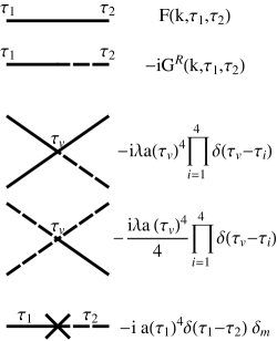
Figure 2: The Feynman rules.

The Feynman rules related to the counter-terms $\delta_{Z}$ and $\delta_{\lambda}$ yield additional powers of the scale factor $a(t)$ and coupling $\lambda$ respectively, and will not contribute to a late time, one-loop computation. Hence we only include the Feynman rule corresponding to $\delta_{m}.$ Since the equal time propagator $G^{R}(x,x)$ vanishes by construction, any non-vanishing one-loop diagram has to have a solid line inside the loop. Thus by the above Feynman rules the only contributions at one-loop level are given in figure 3. According to the Feynman rules, these diagrams contribute

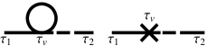
Figure 3: The diagrams contributing to $F(x_{1},x_{2})$ at order $\lambda.$

$$F_{1L}(x_{1},x_{2}) =\int\frac{d^{3}\vec{k}}{(2\pi)^{3}}e^{i\vec{k}\cdot(\vec{x}_{1}-\vec{x}_{2})}F_{1L}(k,\tau_{1},\tau_{2}),\quad{\rm with}$$ (4)

$$F_{1L}(k,\tau_{1},\tau_{2}) =\int d\tau_{v}F(k,\tau_{1},\tau_{v})\left(-iG^{R}(k,\tau_{2},\tau_{v})\right)\left(\mathrm{L}(\tau_{v})+\mathrm{C}(\tau_{v})\right),$$ (5)

$${\rm L}(\tau_{v}) =-i\lambda a(\tau_{v})^{4}\int\frac{d^{3}\vec{p}}{(2\pi)^{3}}F(p,\tau_{v},\tau_{v}),\quad C(\tau_{v})=-ia(\tau_{v})^{4}\delta_{m},$$

where $\mathrm{L}(\tau_{v})$ is the contribution from the amputated one-loop diagram, and $\mathrm{C}(\tau_{v})$ comes from the counter-term diagram.

II.4 The loop contribution

As explained in the introduction, we consider a comoving infrared cut-off $\Lambda_{{\rm IR}}$ and a physical ultraviolet cutoff $\Lambda_{{\rm UV}}$. The contribution from the loop integral can then be written as

$$\mathrm{L}(\tau_{v})=-i\lambda a(\tau_{v})^{4}\left(\int_{\Lambda_{IR}}^{-\tau_{v}^{-1}}+\int_{-\tau_{v}^{-1}}^{\Lambda_{UV}a(\tau_{v})}\right)\frac{dp}{(2\pi)^{2}}2p^{2}F(p,\tau_{v},\tau_{v}),$$ (6)

where we split the integral into parts corresponding to modes inside and outside the horizon at time $\tau_{v}$. In these regions the propagators can be expanded using the mode functions (3) as

$$\textrm{Outside: }|k\tau_{i}|\ll 1 \quad\left\{\begin{array}[]{l}F(k,\tau_{1},\tau_{2})\approx\frac{H^{2}}{2k^{3}}(k^{2}\tau_{1}\tau_{2})^{\epsilon},\\ G^{R}(k,\tau_{1},\tau_{2})\approx\Theta(\tau_{1}-\tau_{2})\frac{H^{2}}{3}\left[\tau_{1}^{3-\epsilon}\tau_{2}^{\epsilon}-\tau_{2}^{3-\epsilon}\tau_{1}^{\epsilon}\right],\end{array}\right.$$ (9)

$$\textrm{Inside: }|k\tau_{i}|\gg 1 \quad\left\{\begin{array}[]{l}F(k,\tau_{1},\tau_{2})\approx\frac{H^{2}\tau_{1}\tau_{2}}{2k}\cos k(\tau_{1}-\tau_{2}),\\ G^{R}(k,\tau_{1},\tau_{2})\approx\Theta(\tau_{1}-\tau_{2})\frac{H^{2}\tau_{1}\tau_{2}}{k}\sin k(\tau_{1}-\tau_{2}),\end{array}\right.$$ (12)

where $\epsilon\equiv m^{2}/(3H^{2})$ is the mass parameter. Inserting the expansions into the loop integral (6) we get

$${\rm L}(\tau_{v}) \approx\frac{-i\lambda}{(2\pi)^{2}H^{2}\tau_{v}^{4}}\left(\tau_{v}^{2\epsilon}\int_{\Lambda_{IR}}^{-\tau_{v}^{-1}}dp\,\,p^{-1+2\epsilon}+\tau_{v}^{2}\int_{-\tau_{v}^{-1}}^{\Lambda_{UV}a(\tau_{v})}dp\,\,p\right)$$

$$\approx\frac{-i\lambda}{(2\pi)^{2}H^{2}\tau_{v}^{4}}\left(\frac{1-(\Lambda_{{\rm IR}}\tau_{v})^{2\epsilon}}{2\epsilon}+\frac{1}{2}\left(\frac{\Lambda_{{\rm UV}}}{H}\right)^{2}\right).$$ (13)

Note that the integrals are dominated by the IR and UV regions as opposed to the horizon $|p\tau_{v}|\sim 1$, and the approximations (9,12) can be used. In order to cancel the ultraviolet divergence we fix the counter-term coefficient $\delta_{m}$ to be

$$\delta_{m}=-\frac{\lambda H^{2}}{2(2\pi)^{2}}\left[\left(\frac{\Lambda_{UV}}{H}\right)^{2}-\left(\frac{\mu}{H}\right)^{2}\right],$$

where $\mu$ is the renormalization scale. This leads to the contribution

$$\mathrm{L}(\tau_{v})+\mathrm{C}(\tau_{v})=\frac{-i\lambda}{(2\pi)^{2}H^{2}\tau_{v}^{4}}\left(\frac{1-(\Lambda_{{\rm IR}}\tau_{v})^{2\epsilon}}{2\epsilon}+\frac{1}{2}\left(\frac{\mu}{H}\right)^{2}\right)\equiv\frac{-i\lambda}{(2\pi)^{2}H^{2}\tau_{v}^{4}}\mathrm{V}(\tau_{v}).$$ (14)

II.5 The propagator at late times

We then wish to analyze the late time dependence of the propagator (4). Inserting the loop contribution (14) we get

$$F_{1L}(x_{1},x_{2})=\frac{-\lambda}{(2\pi)^{2}H^{2}}\int\frac{d^{3}\vec{k}}{(2\pi)^{3}}e^{i\vec{k}\cdot(\vec{x}_{1}-\vec{x}_{2})}\int\frac{d\tau_{v}}{\tau_{v}^{4}}F(k,\tau_{1},\tau_{v})G^{R}(k,\tau_{2},\tau_{v})\mathrm{V}(\tau_{v}).$$ (15)

The integration region naturally splits into components depending on whether mode $k$ is inside or outside the horizon, as indicated in figure 4. In the following we will take $\tau_{1}<\tau_{2}$ for convenience, and also assume that they are in the same cosmological period, $\tau_{1}\sim\tau_{2}\sim\tau_{\mathrm{now}}.$ The limit $\tau_{2}\gg\tau_{1}$ is also of interest, and we will treat it separately in the following.

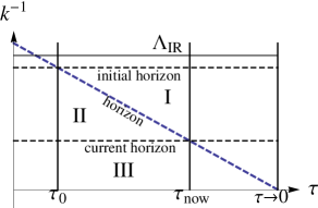
Figure 4: Plot of the integration region in $(\tau,k)$-space.

The IR modes:

Region I consists of modes outside the horizon. Using the expansions (9) we find the momentum space propagator to be

$$F_{1L}^{I}(k,\tau_{1},\tau_{2})=-\frac{\lambda H^{2}}{(2\pi)^{2}}\int_{\tau_{X}}^{\tau_{2}}\frac{d\tau_{v}}{\tau_{v}^{4}}\frac{(k^{2}\tau_{1}\tau_{v})^{\epsilon}}{2k^{3}}\frac{1}{3}\left[\tau_{2}^{3-\epsilon}\tau_{v}^{\epsilon}-\tau_{v}^{3-\epsilon}\tau_{2}^{\epsilon}\right]\mathrm{V}(\tau_{v}),$$

where the lower limit of integration is given by $\tau_{X}\equiv{\rm Max}(\tau_{0},-k^{-1})$, see figure 4. This can be evaluated analytically, yielding

$$F_{1L}^{I}(k,\tau_{1},\tau_{2})=-\frac{\lambda H^{2}}{(2\pi)^{2}}\frac{(k^{2}\tau_{1}\tau_{2})^{\epsilon}}{6k^{3}}\left\{\frac{(\Lambda_{IR}\tau_{2})^{2\epsilon}}{2\epsilon}\left[\frac{1-\left(\frac{\tau_{2}}{\tau_{X}}\right)^{3-4\epsilon}}{3-4\epsilon}+\frac{1-\left(\frac{\tau_{X}}{\tau_{2}}\right)^{2\epsilon}}{2\epsilon}\right]\right.$$

$$\left.-\left(\frac{1}{2}\left(\frac{\mu}{H}\right)^{2}+\frac{1}{2\epsilon}\right)\left(\frac{1-\left(\frac{\tau_{2}}{\tau_{X}}\right)^{3-2\epsilon}}{3-2\epsilon}-\log\frac{\tau_{X}}{\tau_{2}}\right)\right\}\equiv-\frac{\lambda H^{2}}{(2\pi)^{2}}\frac{(k^{2}\tau_{1}\tau_{2})^{\epsilon}}{6k^{3}}D(\tau_{X}).$$ (16)

Transforming back to position space we have

$$F_{1L}^{I}(x_{1},x_{2}) =\int\frac{d^{3}\vec{k}}{(2\pi)^{3}}e^{i\vec{k}\cdot(\vec{x}_{1}-\vec{x}_{2})}F_{1L}^{I}(k,\tau_{1},\tau_{2})=\frac{2}{(2\pi)^{2}}\int_{\Lambda_{IR}}^{-\tau_{2}^{-1}}dk\frac{\sin(k\Delta x)}{k\Delta x}k^{2}F_{1L}^{I}(k,\tau_{1},\tau_{2})$$

$$\approx\frac{2}{(2\pi)^{2}}\int_{\Lambda_{IR}}^{-\tau_{2}^{-1}}dkk^{2}F_{1L}^{I}(k,\tau_{1},\tau_{2})(1+\mathcal{O}((k\Delta x)^{2}),$$

where $\Delta x\equiv|\vec{x}_{1}-\vec{x}_{2}|,$ and in the last step we took the physical separation between $\vec{x}_{1}$ and $\vec{x}_{2}$ to be much less than the Hubble distance. Inserting (16) we find

$$F_{1L}^{I}(x_{1},x_{2}) =-\frac{\lambda H^{2}(\tau_{1}\tau_{2})^{\epsilon}}{(2\pi)^{4}}\int_{\Lambda_{{\rm IR}}}^{-\tau_{2}^{-1}}dk\frac{k^{2\epsilon}}{3k}D(\max(\tau_{0},-k^{-1}))$$

$$=-\frac{\lambda H^{2}(\tau_{1}\tau_{2})^{\epsilon}}{3(2\pi)^{4}}\left(D(\tau_{0})\int_{\Lambda_{{\rm IR}}}^{-\tau_{0}^{-1}}dkk^{-1+2\epsilon}+\int_{-\tau_{0}^{-1}}^{-\tau_{2}^{-1}}dkk^{-1+2\epsilon}D(-k^{-1})\right).$$ (17)

The first integral is over modes outside the horizon already at $\tau_{0}$, and vanishes if one takes the cut-off to coincide with the initial horizon. The integrals can be computed analytically to yield for late times

$$F_{1L}^{I}(x_{1},x_{2}) =-\frac{\lambda H^{2}}{12(2\pi)^{4}\epsilon}\left\{\left(\frac{\tau_{1}\tau_{2}}{\tau_{0}^{2}}\right)^{\epsilon}\log\frac{\tau_{0}}{\tau_{2}}\left[\left(\frac{\mu}{H}\right)^{2}+\frac{1}{\epsilon}\right]\left(1-(\Lambda_{{\rm IR}}\tau_{0})^{2\epsilon}\right)\right.$$

$$\left.+\frac{(\Lambda_{{\rm IR}}^{2}\tau_{1}\tau_{2})^{\epsilon}}{\epsilon}\log\frac{\tau_{0}}{\tau_{2}}+\frac{1}{2\epsilon}\left(\frac{\tau_{1}}{\tau_{2}}\right)^{\epsilon}\left[\left(\frac{\mu}{H}\right)^{2}+\frac{1}{\epsilon}\right]\left(1-\left(\frac{\tau_{2}}{\tau_{0}}\right)^{2\epsilon}\right)\right\}.$$ (18)

The first two terms vanish for late times, while the last one asymptotes to a constant value that is independent of the infrared cutoff $\Lambda_{{\rm IR}}$.

The last term in (18) looks worrisome, as it is divergent in the limit where one takes the leg $\tau_{2}$ to future infinity while keeping the other leg $\tau_{1}$ fixed. This is due to our assumption that the legs are in the same cosmological period, which no longer holds when $\tau_{2}$ is taken to the far-future. The divergence arises because the horizons at $\tau_{2}$ and $\tau_{1}$ no longer coincide in this limit, but rather modes exit the $\tau_{1}$ horizon earlier than the $\tau_{2}$ horizon. In the limit $\tau_{2}\to 0$ with $\tau_{1}$ fixed, with the correct expansions (9,12), the propagator (15) becomes

$$F_{1L}^{\mathrm{I}}(x_{1},x_{2})\approx\frac{\lambda H^{2}}{(2\pi)^{2}}\frac{(\tau_{1}\tau_{2})^{\epsilon}}{3}\left[\frac{(\Lambda_{IR}\tau_{1})^{2\epsilon}}{(2\epsilon)^{2}}+\frac{1}{2}\left(\left(\frac{\mu}{H}\right)^{2}+\frac{1}{\epsilon}\right)\log\frac{\tau_{1}}{\tau_{2}}\right]\left(\cos 1+\mathcal{O}(\epsilon)\right),$$

which is well-behaved for $\tau_{2}\to 0$.

The intermediate region:

Region II consists of modes that are outside the current horizon, but were inside the horizon at the time of the interaction, $\tau_{v}$. Using the relevant expansions for the mode functions (3) we find the momentum space propagator

$$F_{1L}^{II}(k,\tau_{1},\tau_{2})\approx-\frac{\lambda H^{2}}{(2\pi)^{2}}\frac{(k^{2}\tau_{1}\tau_{2})^{\epsilon}}{4k^{4}}\int_{\tau_{0}}^{-k^{-1}}\frac{d\tau_{v}}{\tau_{v}^{2}}\sin(2k\tau_{v}-\pi\epsilon)\left[\frac{1-(\Lambda_{IR}\tau_{v})^{2\epsilon}}{2\epsilon}+\frac{1}{2}\left(\frac{\mu}{H}\right)^{2}\right]$$

$$\approx-\frac{\lambda H^{2}}{(2\pi)^{2}}\frac{(k^{2}\tau_{1}\tau_{2})^{\epsilon}}{4k^{3}}\left[\left(\frac{1}{2}\left(\frac{\mu}{H}\right)^{2}+\frac{1}{2\epsilon}\right)\int_{1}^{\infty}\frac{ds}{s^{2}}\sin(2s-\pi\epsilon)-\frac{\left(\frac{\Lambda_{IR}}{k}\right)^{2\epsilon}}{2\epsilon}\int_{1}^{\infty}\frac{ds}{s^{2-2\epsilon}}\sin(2s-\pi\epsilon)\right],$$

where in the second line we changed variables $s\equiv-k\tau_{v},$ and as the main contribution to the integral comes from the lower limit, we moved the upper limit to infinity. Written thus, the two remaining integrals match to the leading order in $\epsilon$, yielding $I\equiv\int_{1}^{\infty}\frac{ds}{s^{2}}\sin(2s-\pi\epsilon)\approx 0.063+\mathcal{O}(\epsilon)$. Converting back to position space we then have

$$F_{1L}^{II}(x_{1},x_{2}) \approx-\frac{\lambda H^{2}I}{(2\pi)^{4}}\frac{(\tau_{1}\tau_{2})^{\epsilon}}{2}\int_{-\tau_{0}^{-1}}^{-\tau_{2}^{-1}}dk\left[\left(\frac{1}{2}\left(\frac{\mu}{H}\right)^{2}+\frac{1}{2\epsilon}\right)k^{-1+2\epsilon}-\frac{\Lambda_{IR}^{2\epsilon}}{2\epsilon}k^{-1}\right]$$

$$\approx -\frac{\lambda H^{2}I}{8(2\pi)^{4}\epsilon}\left(\frac{\tau_{1}}{\tau_{2}}\right)^{\epsilon}\left[\left(\left(\frac{\mu}{H}\right)^{2}+\frac{1}{\epsilon}\right)\left(1-\left(\frac{\tau_{2}}{\tau_{0}}\right)^{2\epsilon}\right)-2(\Lambda_{IR}\tau_{0})^{2\epsilon}\left(\frac{\tau_{2}}{\tau_{0}}\right)^{2\epsilon}\log\frac{\tau_{0}}{\tau_{2}}\right].$$

This result should be contrasted with the infrared contribution (18). Both asymptote to a constant value for very late times, but the IR contribution is dominant due to an extra factor of $\epsilon^{-1}.$ One can again verify that the apparent divergence as $\tau_{2}\to 0$ with $\tau_{1}$ fixed is due to the assumption $\tau_{1}\sim\tau_{2}$, and vanishes as one computes the potentially divergent part more carefully.

The UV modes:

Finally, in region III the scale $k$ is inside the current horizon between $\tau_{0}$ and $\tau_{{\rm 2}}$. Using the expansion (12) the contribution to the propagator (5) becomes

$$F_{1L}^{III}(k,\tau_{1},\tau_{2}) \approx-\frac{\lambda H^{2}}{(2\pi)^{2}}\frac{\tau_{1}\tau_{2}}{2k^{2}}\int_{\tau_{0}}^{\tau_{2}}\frac{d\tau_{v}}{\tau_{v}^{2}}\cos k(\tau_{1}-\tau_{v})\sin k(\tau_{2}-\tau_{v})\left[\frac{1-(\Lambda_{IR}\tau_{v})^{2\epsilon}}{2\epsilon}+\frac{1}{2}\left(\frac{\mu}{H}\right)^{2}\right]$$

$$\approx-\frac{\lambda H^{2}}{(2\pi)^{2}}\frac{\tau_{1}\tau_{2}}{2k}\int_{\infty}^{-k\tau_{2}}\frac{ds}{s^{2}}\cos(s_{1}-s)\sin(s_{2}-s)\left[\frac{1-(\Lambda_{IR}/k)^{2\epsilon}s^{2\epsilon}}{2\epsilon}+\frac{1}{2}\left(\frac{\mu}{H}\right)^{2}\right],$$ (19)

where we again defined $s\equiv-k\tau_{v}$ and moved the upper limit to infinity. To leading order in $\epsilon$ we then find

$$F_{1L}^{III}(k,\tau_{1},\tau_{2}) \approx-\frac{\lambda H^{2}}{(2\pi)^{2}}\frac{\tau_{1}\tau_{2}}{2k}\left[\frac{1-(\Lambda_{IR}\tau_{2})^{2\epsilon}}{2\epsilon}+\frac{1}{2}\left(\frac{\mu}{H}\right)^{2}\right]$$

$$\cdot\left(\cos k(\tau_{1}+\tau_{2})\mathrm{Ci}(-2k\tau_{2})-\sin k(\tau_{1}+\tau_{2})\left(\frac{\pi}{2}+\mathrm{Si}(2k\tau_{2})\right)\right),$$

where the Cosine and Sine integrals are defined as

$$\mathrm{Ci}(x)=-\int_{x}^{\infty}\frac{\cos s}{s}ds,\qquad\mathrm{and\qquad}\mathrm{Si}(x)=\int_{0}^{x}\frac{\sin s}{s}ds.$$

Transforming back to position space we then get

$$F_{1L}^{III}(x_{1},x_{2}) \approx-\frac{\lambda H^{2}}{(2\pi)^{4}}(\tau_{1}\tau_{2})\left[\frac{1-(\Lambda_{IR}\tau_{2})^{2\epsilon}}{2\epsilon}+\frac{1}{2}\left(\frac{\mu}{H}\right)^{2}\right]$$

$$\cdot\int_{-\tau_{2}^{-1}}^{\Lambda_{UV}a(\tau_{2})}dk\;k\left(\cos k(\tau_{1}+\tau_{2})\mathrm{Ci}(2k\tau_{2})-\sin k(\tau_{1}+\tau_{2})\left(\frac{\pi}{2}+\mathrm{Si}(2k\tau_{2})\right)\right)$$

$$\sim-\frac{\lambda H^{2}}{(2\pi)^{4}}\left(\frac{\tau_{1}}{\tau_{2}}\right)\left[\frac{1-(\Lambda_{IR}\tau_{2})^{2\epsilon}}{2\epsilon}+\frac{1}{2}\left(\frac{\mu}{H}\right)^{2}\right].$$

Above, we noted that the upper limit of the integral doesn’t contribute due to the oscillatory nature of the integrand, and then obtained a rough estimate of the magnitude of the integral by the value of the integrand at the lower limit multiplied by frequency of oscillation. We again find a contribution that asymptotes to a constant for very late times, but is sub-dominant to the infrared and intermediate contributions found above.

II.6 The one-loop propagators

We can now write down the propagators to one loop using the results above. The tree level contributions from the infrared modes (9) to the propagators can be written as

$$F_{0L}(x_{1},x_{2}) =\int\frac{d^{3}\vec{k}}{(2\pi)^{3}}e^{i\vec{k}\cdot(\vec{x}_{1}-\vec{x}_{2})}F(k,\tau_{1},\tau_{2})\approx\frac{H^{2}}{(2\pi)^{2}}(\tau_{1}\tau_{2})^{\epsilon}\int_{\Lambda_{IR}}^{\min(-\tau_{1}^{-1},-\tau_{2}^{-1})}dk\>k^{-1+2\epsilon}$$ (20)

$$\approx\frac{H^{2}}{(2\pi)^{2}}\left(\frac{\tau_{1}\tau_{2}}{\min(\tau_{1},\tau_{2})^{2}}\right)^{\epsilon}\frac{1-(\Lambda_{IR}\min(\tau_{1},\tau_{2}))^{2\epsilon}}{2\epsilon},$$

$$G^{R}(x_{1,}x_{2}) \approx\frac{2H^{2}}{3(2\pi)^{2}}\theta(\tau_{1}-\tau_{2})\left(\tau_{1}^{3-\epsilon}\tau_{2}^{\epsilon}-\tau_{1}^{\epsilon}\tau_{2}^{3-\epsilon}\right)\int_{\Lambda_{IR}}^{-\tau_{1}^{-1}}dk\>k^{2}$$

$$\approx-\frac{2H^{2}}{9(2\pi)^{2}}\theta(\tau_{1}-\tau_{2})\left(\frac{\tau_{2}}{\tau_{1}}\right)^{\epsilon}\left(1-\left(\frac{\tau_{2}}{\tau_{1}}\right)^{3-2\epsilon}\right).$$ (21)

Adding the dominant one loop IR contribution (18) to the tree contribution $F_{0L}(x_{1},x_{2})$, we find the full propagator for late times as

$$F(x_{1},x_{2})\approx\frac{H^{2}}{(2\pi)^{2}}\frac{1}{2\epsilon}\left(1-\frac{\lambda}{12(2\pi)^{2}\epsilon}\left[\left(\frac{\mu}{H}\right)^{2}+\frac{1}{\epsilon}\right]\left(\left(\frac{\tau_{1}}{\tau_{2}}\right)^{\epsilon}+\left(\tau_{1}\leftrightarrow\tau_{2}\right)\right)\right),$$ (22)

where the symmetrization $\tau_{1}\leftrightarrow\tau_{2}$ corresponds to including the mirror images of the diagrams in figure 3. This shows that for a massive field (where $\epsilon>0$) the comoving infrared cutoff $\Lambda_{IR}$ drops out of the late time correlators, which match those obtained from a Bunch-Davies/Euclidean vacuum computation.

II.7 Early time propagator

We should contrast the propagator found above with the corresponding result for early times or very light fields. The infrared contribution to the tree level propagator for light (or massless) fields can be computed from (20) by a power series expansion in $\epsilon$ as

$$F_{0L}^{\mathrm{early}}(x_{1},x_{2}) \approx\frac{H^{2}}{(2\pi)^{2}}\left(\log(\Lambda_{IR}\tau_{0})+\log\left(\frac{\min(\tau_{1},\tau_{2})}{\tau_{0}}\right)\right)\left(1+\mathcal{O}(\epsilon)\right),$$ (23)

where the first logarithm measures how far the infrared cutoff is from the initial horizon, and the second logarithm gives the number of e-folds of inflation. The one-loop correction can be similarly computed by expanding (17) as a power series in $\epsilon.$ After some algebra this gives

$$F_{1L}^{I}(x_{1},x_{2}) \approx\frac{\lambda H^{2}}{9(2\pi)^{4}}\left[\log^{3}\frac{\tau_{2}}{\tau_{0}}+3\log^{2}\frac{\tau_{2}}{\tau_{0}}\left(\log(\Lambda_{IR}\tau_{0})-\frac{1}{8}\left(\frac{\mu}{H}\right)^{2}\right)\right.$$

$$-\frac{1}{4}\log\frac{\tau_{2}}{\tau_{1}}\left(\left(\frac{\mu}{H}\right)^{2}+\log(\Lambda_{IR}\tau_{0})\left(\frac{3}{4}\left(\frac{\mu}{H}\right)^{2}-3\log(\Lambda_{IR}\tau_{0})\right)\right)$$

$$+\left.\log(\Lambda_{IR}\tau_{0})\left(\log(\Lambda_{IR}\tau_{0})-\frac{1}{8}\left(\frac{\mu}{H}\right)^{2}\right)-\frac{1}{12}\left(\frac{\mu}{H}\right)^{2}\right]\left(1+\mathcal{O}(\epsilon)\right).$$ (24)

These results showcase the familiar logarithmic divergences for late times $\tau_{2}\to 0$, but as shown earlier, these are absent for truly late times if $\epsilon>0$. The solution to this apparent paradox is that the expansions in (23), (24) are valid when $\epsilon\ll 1/\log\left(\tau_{0}/\tau_{2}\right),$ which means the logarithmic expansion breaks down for sufficiently late times, and the propagator is better described by (22), which is well behaved.

III DISCUSSION AND CONCLUSIONS

Massive scalar

We conclude from section II.6 that in the distant future, the loop corrections are insensitive to the choice of infrared cutoff. The result for the comoving cutoff approaches that of the de Sitter invariant Euclidean vacuum results as $\tau_{2}^{2\epsilon}$ , i.e. as a negative power of the scale factor.

Massless scalar, or a light scalar at early times

Here the result of section II.7 is applicable. This can be the relevant behavior during the entire course of slow roll inflation. The difference between the result of section II.7 and section II.6 provides a measure of the theoretical uncertainty in the predictions of the two-point function caused by uncertainties in the initial state at the start of inflation. This difference is proportion to a $\lambda\log^{2}\left(\tau_{2}/\tau_{0}\right)\log\left(\Lambda_{IR}\tau_{0}\right)$ relative to the tree level contribution. The slow roll conditions for pure $\lambda\phi^{4}$ give the constraint that the initial expectation value for $\phi$ must be larger than the Planck scale. The condition that the density fluctuations today be sufficiently small $(10^{-5})$ gives the constraint that $\lambda\approx 10^{-15}$. So we see in this example the effect will be at least $10^{-11}$ smaller than the tree-level piece, even after 60 e-folds of inflation. We conclude therefore, that while these secular logarithms are present during primordial slow-roll inflation, matching the magnitude of our observed density perturbations constrains the parameters of the inflaton model such that the coefficient of the secular log is very small, unless inflation is very long-lived.

Massless scalar at late times

The Euclidean vacuum methods break down in this case (see for example Hollands (2011) for a recent discussion of this situation) due to the nonexistence of a de Sitter invariant vacuum for a massless scalar Allen (1985). However the comoving IR cutoff approach still provides a well-defined perturbative expansion, up until the point when $\lambda\log^{3}\left(\tau_{2}/\tau_{0}\right)\sim 1$ (see (24)). The prediction is that the theoretical uncertainty in correlators becomes large at sufficiently late times. This is the practical sense in which de Sitter spacetime suffers a quantum instability. In the slow roll example, this does not happen until about $10^{5}$ e-folds, so is really only of academic interest as far as primordial inflation goes.

Graviton at late times

However it should be noted our result for the massless scalar matches qualitatively with the computation of Tsamis and Woodard (1996). There the full one-loop correction for graviton self-energy was computed with the same kind of comoving infrared cutoff that we have used in the present paper. Compared to the tree-level result the contribution is of order $\left(\frac{H}{M_{pl}}\right)^{4}\log^{2}\left(\tau_{2}/\tau_{0}\right)$. Again this is very small over the 60 e-folds needed for primordial inflation. However over the present epoch such a term may become important, if we are indeed evolving toward a period where dark energy dominates. To apply these ideas to our present epoch, we could imagine simply shifting $\tau_{0}$ to the present time, and placing a comoving infrared cutoff just outside our present horizon. This suggests quantum uncertainties due to the indeterminancy of our initial state would only become large after $\left(\frac{M_{pl}}{H_{0}}\right)^{2}\approx 10^{122}$ e-folds of late time expansion, where now $H_{0}\approx 10^{-33}$ eV is the Hubble parameter today. It is interesting that this provides a mechanism for the possible breakdown of semiclassical physics in a de Sitter region, as predicted by quantum gravity arguments in Lowe and Roy (2010).

References

• Friedrich (1986) H. Friedrich, “On The Existence Of N-Geodesically Complete Or Future Complete Solutions Of Einstein Field-Equations With Smooth Asymptotic Structure”, Communications In Mathematical Physics 107 (1986), no. 4, 587–609.
• Friedrich (1986) H. Friedrich, “Existence and structure of past asymptotically simple solutions of einstein’s field equations with positive cosmological constant”, Journal of Geometry and Physics 3 (1986), no. 1, 101 – 117.
• Friedrich (1991) H. Friedrich, “On the global existence and the asymptotic behavior of solutions to the Einstein-Maxwell-Yang-Mills equations”, J.Diff.Geom. 34 (1991) 275–345.
• Traschen and Hill (1986) J. H. Traschen and C. Hill, “Instability Of De Sitter Space On Short Time Scales”, Phys.Rev. D33 (1986) 3519–3525.
• Tsamis and Woodard (1993) N. Tsamis and R. Woodard, “Relaxing the cosmological constant”, Phys.Lett. B301 (1993) 351–357.
• Brandenberger et al. (1993) R. H. Brandenberger, H. Feldman, and V. F. Mukhanov, “Classical and quantum theory of perturbations in inflationary universe models”, arXiv:astro-ph/9307016.
• Tsamis and Woodard (1995) N. Tsamis and R. Woodard, “Strong infrared effects in quantum gravity”, Annals Phys. 238 (1995) 1–82.
• Tsamis and Woodard (1997) N. Tsamis and R. Woodard, “The Quantum gravitational back reaction on inflation”, Annals Phys. 253 (1997) 1–54, arXiv:hep-ph/9602316.
• Tsamis and Woodard (1996) N. Tsamis and R. Woodard, “Quantum gravity slows inflation”, Nucl.Phys. B474 (1996) 235–248, arXiv:hep-ph/9602315.
• Mukhanov et al. (1997) V. F. Mukhanov, L. W. Abramo, and R. H. Brandenberger, “On the Back reaction problem for gravitational perturbations”, Phys.Rev.Lett. 78 (1997) 1624–1627, arXiv:gr-qc/9609026.
• Abramo et al. (1997) L. W. Abramo, R. H. Brandenberger, and V. F. Mukhanov, “The Energy - momentum tensor for cosmological perturbations”, Phys.Rev. D56 (1997) 3248–3257, arXiv:gr-qc/9704037.
• Abramo and Woodard (1999) L. Abramo and R. Woodard, “One loop back reaction on chaotic inflation”, Phys.Rev. D60 (1999) 044010, arXiv:astro-ph/9811430.
• Weinberg (2005) S. Weinberg, “Quantum contributions to cosmological correlations”, Phys.Rev. D72 (2005) 043514, arXiv:hep-th/0506236.
• Weinberg (2006) S. Weinberg, “Quantum contributions to cosmological correlations. II. Can these corrections become large?”, Phys.Rev. D74 (2006) 023508, arXiv:hep-th/0605244.
• Polyakov (2006) A. Polyakov, “Beyond space-time”, arXiv:hep-th/0602011.
• van der Meulen and Smit (2007) M. van der Meulen and J. Smit, “Classical approximation to quantum cosmological correlations”, JCAP 0711 (2007) 023, arXiv:0707.0842.
• Bartolo et al. (2008) N. Bartolo, S. Matarrese, M. Pietroni, A. Riotto, and D. Seery, “On the Physical Significance of Infra-red Corrections to Inflationary Observables”, JCAP 0801 (2008) 015, arXiv:0711.4263.
• Polyakov (2008) A. Polyakov, “De Sitter space and eternity”, Nucl.Phys. B797 (2008) 199–217, arXiv:0709.2899.
• Adshead et al. (2009) P. Adshead, R. Easther, and E. A. Lim, “The ’in-in’ Formalism and Cosmological Perturbations”, Phys.Rev. D80 (2009) 083521, arXiv:0904.4207.
• Burgess et al. (2010) C. Burgess, L. Leblond, R. Holman, and S. Shandera, “Super-Hubble de Sitter Fluctuations and the Dynamical RG”, JCAP 1003 (2010) 033, arXiv:0912.1608.
• Polyakov (2010) A. Polyakov, “Decay of Vacuum Energy”, Nucl.Phys. B834 (2010) 316–329, arXiv:0912.5503.
• Krotov and Polyakov (2011) D. Krotov and A. M. Polyakov, “Infrared Sensitivity of Unstable Vacua”, Nucl.Phys. B849 (2011) 410–432, arXiv:1012.2107.
• Tsamis and Woodard (1996) N. Tsamis and R. Woodard, “One loop graviton selfenergy in a locally de Sitter background”, Phys.Rev. D54 (1996) 2621–2639, arXiv:hep-ph/9602317.
• Seery (2010) D. Seery, “Infrared effects in inflationary correlation functions”, Class.Quant.Grav. 27 (2010) 124005, arXiv:1005.1649.
• Kahya et al. (2010) E. Kahya, V. Onemli, and R. Woodard, “A Completely Regular Quantum Stress Tensor with w < -1”, Phys.Rev. D81 (2010) 023508, arXiv:0904.4811.
• Kundu (2011) S. Kundu, “Inflation with General Initial Conditions for Scalar Perturbations”, arXiv:1110.4688.
• Kolb and Turner (1990) E. W. Kolb and M. S. Turner, “The Early universe”, Front.Phys. 69 (1990) 1–547.
• Lyth (2007) D. H. Lyth, “The curvature perturbation in a box”, JCAP 0712 (2007) 016, arXiv:0707.0361.
• Lowe (2008) D. A. Lowe, “Some comments on embedding inflation in the AdS/CFT correspondence”, Phys.Rev. D77 (2008) 066003, arXiv:0710.3564.
• Lowe and Roy (2010) D. A. Lowe and S. Roy, “Punctuated eternal inflation via AdS/CFT”, Phys.Rev. D82 (2010) 063508, arXiv:1004.1402.
• Enqvist et al. (2008) K. Enqvist, S. Nurmi, D. Podolsky, and G. Rigopoulos, “On the divergences of inflationary superhorizon perturbations”, JCAP 0804 (2008) 025, arXiv:0802.0395.
• Maciejko (2007) J. Maciejko, “An introduction to non-equilibrium many-body theory”, 2007, unpublished.
• Hollands (2011) S. Hollands, “Massless interacting quantum fields in deSitter spacetime”, arXiv:1105.1996.
• Allen (1985) B. Allen, “Vacuum States in de Sitter Space”, Phys. Rev. D32 (1985) 3136.
• Adler (1972) S. L. Adler, “Massless, Euclidean quantum electrodynamics on the five- dimensional unit hypersphere”, Phys. Rev. D6 (1972) 3445–3461.
• Adler (1973) S. L. Adler, “Massless Electrodynamics On The Five-Dimensional Unit Hypersphere: An Amplitude - Integral Formulation”, Phys. Rev. D8 (1973) 2400–2418.
• Drummond (1975) I. T. Drummond, “Dimensional Regularization of Massless Theories in Spherical Space-Time”, Nucl. Phys. B94 (1975) 115.
• Drummond and Shore (1979a) I. T. Drummond and G. M. Shore, “Conformal Anomalies for Interacting Scalar Fields in Curved Space-Time”, Phys. Rev. D19 (1979)a 1134.
• Drummond and Shore (1979b) I. T. Drummond and G. M. Shore, “Dimensional Regularization of Massless Quantum Electrodynamics in Spherical Space-Time. 1”, Ann. Phys. 117 (1979)b 89.
• Marolf and Morrison (2011) D. Marolf and I. A. Morrison, “The IR stability of de Sitter QFT: results at all orders”, Phys. Rev. D84 (2011) 044040, arXiv:1010.5327.
• Marolf and Morrison (2010) D. Marolf and I. A. Morrison, “The IR stability of de Sitter: Loop corrections to scalar propagators”, Phys. Rev. D82 (2010) 105032, arXiv:1006.0035.
• Hollands (2010) S. Hollands, “Correlators, Feynman diagrams, and quantum no-hair in deSitter spacetime”, arXiv:1010.5367.
• Marolf and Morrison (2011) D. Marolf and I. A. Morrison, “The IR stability of de Sitter QFT: Physical initial conditions”, arXiv:1104.4343.
• Starobinsky (1986) A. A. Starobinsky, “Stochastic De Sitter (Inflationary) Stage In The Early Universe”, 1986.
• Starobinsky and Yokoyama (1994) A. A. Starobinsky and J. Yokoyama, “Equilibrium state of a selfinteracting scalar field in the De Sitter background”, Phys.Rev. D50 (1994) 6357–6368, arXiv:astro-ph/9407016.
• Coleman and De Luccia (1980) S. R. Coleman and F. De Luccia, “Gravitational Effects on and of Vacuum Decay”, Phys.Rev. D21 (1980) 3305.
• Goldstein and Lowe (2003) K. Goldstein and D. A. Lowe, “Initial state effects on the cosmic microwave background and trans-planckian physics”, Phys. Rev. D67 (2003) 063502, hep-th/0208167.
• Goldstein and Lowe (2004) K. Goldstein and D. A. Lowe, “Real-time perturbation theory in de Sitter space”, Phys. Rev. D69 (2004) 023507, hep-th/0308135.
• Goldstein and Lowe (2003) K. Goldstein and D. A. Lowe, “A note on alpha-vacua and interacting field theory in de Sitter space”, Nucl. Phys. B669 (2003) 325–340, hep-th/0302050.