Quantum Control Experiments as a Testbed for Evolutionary Multi-Objective Algorithms

Abstract

Experimental multi-objective Quantum Control is an emerging topic within the broad physics and chemistry applications domain of controlling quantum phenomena. This realm offers cutting edge ultrafast laser laboratory applications, which pose multiple objectives, noise, and possibly constraints on the high-dimensional search. In this study we introduce the topic of Multi-Observable Quantum Control (MOQC), and consider specific systems to be Pareto optimized subject to uncertainty, either experimentally or by means of simulated systems. The latter include a family of mathematical test-functions with a practical link to MOQC experiments, which are introduced here for the first time. We investigate the behavior of the multi-objective version of the Covariance Matrix Adaptation Evolution Strategy (MO-CMA-ES) and assess its performance on computer simulations as well as on laboratory closed-loop experiments. Overall, we propose a comprehensive study on experimental evolutionary Pareto optimization in high-dimensional continuous domains, draw some practical conclusions concerning the impact of fitness disturbance on algorithmic behavior, and raise several theoretical issues in the broad evolutionary multi-objective context.

Keywords:

Experimental Pareto optimization, Quantum Control experiments, robustness to noise, multi-objective evolution strategies, covariance matrix adaptation, diffraction grating.

1 Introduction

Quantum Control (QC) [1, 2], sometimes referred to as Optimal Control or Coherent Control, aims at altering the course of quantum dynamics phenomena for specific target realizations. There are two main threads within QC, theoretical and experimental control, as typically encountered in physics. Interest in the subject has rapidly increased during the past 10 years, in parallel with the technological developments of ultrafast laser pulse shaping capabilities [3] that made it possible to bring the dream into experimental fruition.

Quantum Control Theory (QCT) [4] aims at manipulating the quantum dynamics of a simulated system by means of an external control field, which typically corresponds to a temporal electromagnetic field arising from a laser source. Quantum Control Experiments (QCE) [5] consider the realization of QC in the laboratory, generally executed by applying evolutionary learning-loops for altering the course of quantum dynamics phenomena. Here, the yield, or success-rate, is assessed by a physical measurement. The nature of the optimization is fundamentally different than in QCT, due to practical laboratory constraints: limited bandwidth, limited fluence, control resolution, proper control basis, etc.
The optimization of QC systems in the laboratory typically poses many algorithmic challenges, such as operating with high-dimensionality, noise, control constraints, and most importantly in this context, a potentially large number of simultaneous objectives. Attractive features of QCE are the extremely short duration and low cost of an experiment, in comparison to other real-world experimental systems: the duration of a typical QC measurement is 1msec, allowing a well-averaged single experiment to be recorded in the order of a single second.

Evolutionary Algorithms (EAs) [6] are the most commonly employed routines for optimization of QCE systems. This can mostly be attributed to their high success-rate in addressing the aforementioned challenges, as reported also in other domains of experimental many-parameter systems (see, e.g., [7]). In particular, they efficiently treat noisy problems, likely due to the employment of large populations as well as to the fact that they do not require any explicit gradient determination. Furthermore, EAs possess several features which are very effective in solving multi-objective (MO) problems, such as being population-based algorithms, having diversity generation and preservation mechanisms, etc. Evolutionary Multi-Objective Algorithms (EMOA) (see, e.g., [8, 9, 10]) constitute popular Pareto optimizers that have been highly successful in treating MO problems.

The list of successful quantum systems controlled in the laboratory by means of EAs in physics and chemistry is growing rapidly [2], but the vast majority address de facto single-objective optimization problems. The topic of multi-objective QC, also referred to as Multi-Observable Quantum Control (MOQC), considers multiple distinct physical observables, referring to mutually competing physical processes. One scenario is a single type of quantum system, where the competition may be driven by ratios of controlled ionization or fragmentation of the same molecule [11], versus other scenarios involving several independent quantum systems, e.g., fluorescence signals in Optimal Dynamic Discrimination (ODD) of similar molecules [12, 13]. MOQC has been addressed in various experimental systems, predominantly by means of tailored single-objective scalar functions (see, e.g., [14]). Treating MOQC as a Pareto optimization problem has been reported only recently, and there is currently a limited number of studies on this topic: see [15] for QCT and [12] for QCE. While the former constituted the first theoretical study of Pareto fronts in QC, even without involving a MO algorithmic approach, the latter study is the first reported experimental QC work by means of an EMOA, namely the NSGA-II [8].

This study considers several MOQC systems, both experimental systems in the laboratory as well as simulated systems subject to noisy environments. This work aims to present a pioneering study on experimental Pareto optimization in high-dimensional continuous domains (at least $n=80$ decision parameters). Following the successful application of the Covariance Matrix Adaptation Evolution Strategy (CMA-ES) [16] to single-objective QC systems [17, 18], the current study focuses on the multi-objective version of the CMA-ES (referred to in our notation as MO-CMA) [19] as the algorithmic tool. We investigate its performance upon treating optimization tasks of both noisy model landscapes (e.g., Multi-Sphere) as well as real-world MOQC systems.

The manuscript is organized as follows. Section 2 will provide some background on the study of EMOA under noise, and outline the specific characteristics of QCE systems in this context. This will be followed by the description of our algorithmic scheme in Section 3, where we shall also discuss the topic of single-parent elitist ES behavior in the presence of noise. Section 4 will introduce the systems under study. We will report on our practical observations in Section 5, and conclude in Section 6.

2 Uncertain Environments (Noise)

The presence of uncertainties in environments subject to optimization by EAs has been widely studied in recent years. The traditional classes of investigated uncertainties typically include noisy objective functions [20], approximation error in the objective function [21], the search for robust solutions [22], and dynamic environments [23]. Optimization subject to noisy environments is typically defined within the topic of Robustness. While the research on single-objective EAs under uncertain environments in general, and under noisy objective functions in particular, has been widely studied (see, e.g., [20, 24]), there is a limited number of reported EMOA studies to date. The vast majority of the existing studies consider the scenario of fitness functions subject to noise, and propose techniques to efficiently handle this particular uncertainty. Such studies typically make the assumption that the fitness values are subject to additive Gaussian noise, denoted by $\mathcal{N}$, with zero mean and finite variance,

$$\tilde{f}_{i}\left(\vec{x}\right)=f_{i}\left(\vec{x}\right)+\mathcal{N}\left(0,\epsilon_{f}^{2}\right),$$ (1)

where the perceived $i^{th}$ fitness is $\tilde{f}_{i}$ and the ideal fitness is $f_{i}$. The variance of the normal disturbance, $\epsilon_{f}^{2}$, is referred to as the noise strength, and is assumed to either remain fixed during a run (i.e., additive noise), or to be a multiplicative factor of the fitness measurement, i.e., $\epsilon_{f_{i}}^{2}\sim f_{i}$. Also, the so-called degree of overvaluation usually refers to the difference between the perceived fitness and the ideal fitness: $\tilde{f}_{i}-f_{i}$. Other types of noisy models, such as consideration of uncertainty in the decision parameters to be optimized, have received scarce attention [25, 26]. This type of noise, which corresponds to the precision of the optimized design and may represent manufacturing error, is of particular interest to this study. The fitness values are then modeled as

$$\tilde{f}_{i}\left(\vec{x}\right)=f_{i}\left(\vec{x}+\mathcal{N}\left(\vec{0},\epsilon_{x}^{2}\mathbf{I}\right)\right).$$ (2)

Here, since the decision parameters are systematically disturbed, each one of them can be controlled only up to a certain degree of accuracy. Moreover, the fitness values in this case may be either enhanced or deteriorated, depending exclusively upon the nature of the objective function and the manner in which the noise propagates through it. Thus, the expected fitness overvaluation or undervaluation may be estimated only if the propagation of the noise can be derived. We choose to refer here to the difference between the perceived and the ideal fitness values stemming from noisy decision parameters as the fitness disturbance, i.e., $\left|\tilde{f}_{i}-f_{i}\right|$.

Regardless of the differences in the modeling, the system still retains inherent underlying uncertainty, explicitly revealed by two successive evaluations of the same recorded input variables returning two different sets of output values.

2.1 EMOA in Noisy Environments: Robustness

Early EMOA work on treatment of noisy objective functions includes the probabilistic Pareto ranking approach (similar concepts by [27] and [28]), which introduces a modified selection criterion accounting for the stochasticity of the objective function. The concepts of domination dependent lifetime and re-sampling of archived solutions was introduced by Büche et al. in [29]. Moreover, recent studies (see, e.g., [30]) proposed noise-handling features, as additions to existing EMOA, and considered a suite of synthetic bi-criteria landscapes as a testbed. In a recent study, Bader and Zitzler [31] provided an important overview on robustness in multi-objective optimization. In general terms, multi-objective noise-treatment and robustness-accounting are carried out by one of the following schemes [31]:

1. Replacement of the objective function value by a measure reflecting uncertainty, e.g., statistical mean, or signal averaging [32]

2. Introduction of an additional robustness criterion to the search [26, 33, 34]

3. Consideration of a tailored robustness constraint, imposing candidate solutions to satisfy statistical criteria [26, 35]

In what follows, we refer to two specific studies that are directly linked to our work.

Simulated Robustness in Multi-Objective Optimization

Deb and Gupta [26], in a pioneering work, introduced systematic disturbance to decision parameters in Pareto optimization and posed the demand for attaining robust solutions. The study shifted the focus from searching for global best Pareto fronts to robust Pareto fronts, whose pre-images are solutions that are robust to variable perturbations. However, as the authors concluded, the proposed schemes were prone to being impractical in real-world scenarios, as they increased the total number of evaluations by factors of $\sim$ 50–100.

Multi-Objective Experimental Optimization

The first reported campaign of experimental Pareto optimization was carried out by Knowles and co-workers within biological experimental platforms (e.g., [36], and see [37] for an overview). In addition to the successful results on multiple experimental systems, this campaign led to the subsequent development of the ParEGO, an EMOA specializing in Pareto optimization subject to an extremely small budget of measurements (see, e.g., [38]). This promising search heuristic was designed for specific demanding experimental conditions, amongst which are

• low noise levels, i.e., individual experiments practically need not be repeated,

• locally smooth search landscapes,

• low-dimensional search spaces (less than $10$ decision parameters).

Note on Elitism versus Robustness

It has been pointed out in previous studies that elitist selection is an essential component for efficient multi-objective optimization (see, e.g., [39, 40]). A common argument is the need to preserve the current population’s information in the global selection phases of Pareto domination followed by secondary criteria. Elitism, at the same time, dictates a unique dynamic that when exposed to uncertain environments has the potential to deteriorate the quality of the run, suffer from systematic overvaluation, and lead to periods of stagnation. The currently employed EMOA, namely the MO-CMA, employs an elitist strategy as its algorithmic kernel. Due to its nature, and due to the nature of experimental frameworks, we shall also explore theoretical studies from the realm of single-objective Evolution Strategies related to this study, as outlined in Section 3.

2.2 QC Systems: Sources of Noise and Uncertainty

Uncertainty in QCE stems from various sources, and exists at several levels. We attribute it to three main factors, in decreasing importance, as we shall explain in detail in what follows (compare to [22] as a generic reference):

1. Spectral phase noise: uncertainty concerning the decision (input) parameters; the error in realizing the prescribed parameters in the experimental setup

2. Observation noise: uncertainty concerning the measurement (output) values, originating from detector noise (also known as Johnson-Nyquist noise)

3. Environmental drift: Systematic slow deviation in the system values over the time span of the entire experiment, e.g., minutes to hours

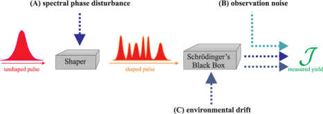
Figure 1: Summary of the three main sources of noise in a typical Quantum Control experiment. Compare to [22] as a generic reference.

(A) The primary component in the current experimental learning loop generating uncertainty with highest impact is the process responsible for the construction of the laser pulse, which is carried out with a pulse shaper. Unlike standard modeling in the literature regarding noisy environments, the current framework is modeled as subject to additive Gaussian noise on the control variables (i.e., the decision parameters to be optimized, or the input), which propagates typically in a highly nonlinear manner to the measured values (i.e., the objective functions, or the outputs). More explicitly, the control function with spectral modulation consists of the spectral amplitude $A(\omega)$ and phase $\phi(\omega)$ functions, which together construct the electric field:

$$E(t)=\mathbb{R}\left\{\int A(\omega)\exp(i\phi(\omega))\exp(-i\omega t)\ d\omega\right\}.$$ (3)

Most QC processes are highly sensitive to the phase, and phase-only shaping is typically sufficient for attaining optimal control. Our experiments only include phase modulation, where the spectral function $A(\omega)$ is fixed. The latter is well approximated by a Gaussian and determines the bandwidth, or the minimal pulse duration. Note that shaping the field with phase-only modulation guarantees conservation of the pulse energy.

The spectral phase $\phi(\omega)$ is defined at $n$ frequencies $\{\omega_{j}\}_{j=1}^{n}$ that are equally distributed across the bandwidth of the spectrum. These $n$ values, $\{\phi(\omega_{j})\}_{j=1}^{n}$, correspond to the $n$ pixels of the pulse shaper and are the decision parameters to be optimized in the experimental learning loop:

$$\phi\left(\omega\right)=\left(\phi(\omega_{1}),\phi(\omega_{2}),...,\phi(\omega_{n})\right).$$ (4)

The laser field, as defined in Eq. 3, completely determines the dynamics of any controlled quantum process, subject to the associated wavefunction $\psi(t)$, satisfying the Schrödinger equation:

$$\begin{array}[]{l}\displaystyle i\frac{\partial\psi}{\partial t}=(H_{0}+V)\psi(t)\\ \displaystyle V=-\mu E(t)\cos(\omega_{0}t)\end{array}$$ (5)

where $H_{0}$ is the field-free Hamiltonian and $\mu$ is the electric dipole moment. The modeling of noise on the shaper is equivalent to Eq. 2, assuming additive Gaussian noise on each pixel (independent Gaussian sampling):

$$\tilde{\phi}(\omega)=\left(\phi(\omega_{1})+\mathcal{N}_{1}\left(0,\epsilon_{S}^{2}\right),\ldots,\phi(\omega_{n})+\mathcal{N}_{n}\left(0,\epsilon_{S}^{2}\right)\right),$$ (6)

where $\tilde{\phi}(\omega)$ and $\phi(\omega)$ are the perceived and the ideal pixel values, respectively, and each pixel is subject to a noise level of $\epsilon_{S}^{2}$; the latter is assumed to remain fixed during the course of the whole experiment. Since this type of uncertainty stems from physical disturbances – such as dust or convection currents that are responsible for variable refraction indices, and therefore can be modeled as some continuous function – the independently sampled Gaussian disturbance is thus an approximation. The correlations between disturbances on adjacent pixels may be considered in further studies.

The variations in the input propagates into the output in a highly nonlinear manner, due to the complex transformations involved in the process (Eqs. 3 and 5), and yields non-additive deviations with an unknown form.

(B) Given a quantum observable operator, $\mathcal{O}_{i}$, and given the propagated wavefunction $\psi$ solving Eq. 5, a quantum observation is then defined as $\mathcal{J}_{i}=\left<\psi\left|\mathcal{O}_{i}\right|\psi\right>$ . The measurement value is assumed to be subject to observation noise, corresponding to electronic or thermal fluctuations in the detector (Johnson-Nyquist noise), which typically possesses very low noise strength $\epsilon_{\mathcal{J}}^{2}$ and is modeled as additive Gaussian deviations, equivalent to Eq. 1.
The high duty cycle of QC experiments (typically 1kHz) permits increased signal averaging, which reduces the influence of additive noise sources, such as measurement noise, by virtue of the central limit theorem. Thus, given $k$ independent, single-shot measurements, the mean and variance of the observation in the presence of measurement noise, $\tilde{\mathcal{J}}_{i}$, may be described as follows:

$$\left<\tilde{\mathcal{J}}_{i}\right>=\mathcal{J}_{i},~{}~{}~{}\textrm{VAR}\left[\tilde{\mathcal{J}}_{i}\right]=\frac{\epsilon_{\mathcal{J}}^{2}}{k},$$ (7)

and given sufficient signal averaging, its contribution is effectively removed. While such signal averaging always increases the precision of the QC measurement, the contribution of non-additive noise sources, such as the propagation of $\tilde{\phi}(\omega)$ (Eq. 6), may not be removed, and is of particular interest in this study.

(C) The third source of uncertainty, with the least impact, is general system drift which occurs in a time span of the entire experiment (minutes to hours). The observation is then disturbed by some temporal function $\xi(t)$:

$$\hat{\mathcal{J}}_{i}(t)=\tilde{\mathcal{J}}_{i}+\xi(t).$$ (8)

Fig. 1 summarizes the sources of noise in a typical QC experiment.

3 The Algorithmic Approach: Multi-Objective CMA-ES

Following the broad success of the Covariance Matrix Adaptation Evolution Strategy (CMA-ES) in single-objective continuous optimization, a multi-objective version has been released [19]. In short, the CMA is a derandomized ES variant that has been successful in treating correlations among decision parameters by efficiently learning optimal mutation distributions. The MO-CMA relies on the elitist $\left(1+\lambda\right)$-CMA kernel [41] (typically with $\lambda=1$), which had been originally designed for it, likely due to the aforementioned studies indicating that elitism is essential for efficient multi-objective optimization [39, 40]. The elitist CMA combines the classical concepts of the $\left(1+1\right)$-ES, and especially the success probability and the success rule components (see, e.g., [6]), with the Covariance Matrix Adaptation concept.

Explicitly, the set of evolving individuals comprises $\mu$ search points, which correspond to $\mu$ independently evolving single-parent CMA mechanisms. Given the $i^{th}$ search point in generation $g$, $\vec{x}^{(g)}_{i}$, an offspring is generated by means of a Gaussian variation:

$$\vec{x}^{(g+1)}_{i}\sim\mathcal{N}\left(\vec{x}^{(g)}_{i},\sigma^{(g)^{2}}_{i}\mathbf{C}^{(g)}_{i}\right).$$ (9)

The covariance matrices, $\left\{\mathbf{C}^{(g)}_{i}\right\}_{i=1}^{\mu}$, are initialized as unit matrices and are learned during the course of evolution, based on cumulative information of successful past mutations. The step-sizes, $\left\{\sigma^{(g)}_{i}\right\}_{i=1}^{\mu}$, are updated according to the so-called success rule based step-size control. The set of parents and offspring undergoes two MO evaluation phases, corresponding to two selection criteria: the first criterion is Pareto domination ranking, followed by the hypervolume contribution criterion. Fig. 2 illustrates the operation of the MO-CMA algorithm. For more details we refer the reader to [19].

Figure 2: Cartoons illustrating the MO-CMA mechanism: [LEFT] The objective space, where selection is subject to two criteria: Pareto domination ranking and hypervolume contribution [19]. [MIDDLE] The decision (search) space, where the pre-images of the evolving Pareto front are depicted, and simultaneously update as independent (1+1)-CMA kernels. [RIGHT] A solitary CMA kernel evolving in the decision space of an elliptic single-objective model landscape.

3.1 Introduction of Noise

The application of the MO-CMA to MOQC in general, and to the systems under investigation in the current study, introduces new aspects to Pareto optimization at different levels that have to be addressed. The current framework differs from previously studied MO noisy systems in two main aspects:

• The recorded objective function values (signal measurements) cannot be assumed to follow a specific distribution; the degree to which the noise on the decision parameters propagates into the objective function values is generally unknown, and in any case the latter is not additive.

• Due to the nature of the MO-CMA learning rules, any manipulation or replacement of archived solutions is not recommended. This is a common rule of thumb for the family of derandomized ES, which rely on cumulative information gained from previously selected search points.

Furthermore, the introduction of noise to the MO-CMA is expected to raise additional issues:

• Single-parent strategies experience difficulties in handling noisy landscapes, in comparison to multi-parent strategies: the application of recombination in the latter case proved highly efficient in treating excessive noise [42]. More specifically, in the context of QC experimental optimization, the single-objective CMA was observed in [17] to fail without recombination, and to perform extremely well otherwise, as expected from theory [42].

• Elitist strategies support the survival of parents, and are likely to encounter scenarios in which highly overvaluated perceived fitness values are kept for long periods, causing stagnation (see, e.g., [43]). The issue of fitness disturbance is expected to become a problem for the MO-CMA, should its implementation follow the original algorithm and avoid parental fitness re-evaluation.

Arnold and Beyer [44] considered the aforementioned effects and studied theoretically the local performance of the single-objective $(1+1)$-ES in a noisy environment. Here are some of the relevant conclusions of that study:

1. Failure to reevaluate the parental fitness leads to systematic overvaluation.

2. Overvaluation is responsible for the different behavior of the elitist single-parent strategy, in comparison to other strategies, and may lead to long periods of stagnation.

3. Overvaluation may, nevertheless, be beneficial for the specific homogeneous environment of the quadratic sphere in the limit of infinite dimensions.

4. Occasional parental fitness re-evaluation seems to be superior with respect to no re-evaluation at all and to re-evaluation in every generation.

5. Overvaluation has the potential to render useless success-probability based step-size mechanisms.

It should be stressed that disturbance of objective function values in experimental optimization typically cannot be tolerated, and is primarily perceived as a source of deception that deteriorates the reliability of the attained results. Also, the main focus of the current study is on the attained set of solutions, and on the ability to reproduce the perceived fitness values as reported in the algorithm’s output. In particular, in the MO context, the research goal is to investigate the nature of the attained Pareto optimal set, in light of its a posteriori re-evaluation.

3.2 A Proposed Scheme

Given the conclusions concerning the $(1+1)$-ES outlined in the previous section, we would like to propose a modus operandi for our experimental optimization, subject to noise, with the MO-CMA. In particular, three different empirical scenarios are considered:

1. Default MO-CMA (’D’)

2. Parental fitness re-evaluation every generation (’E’)

3. Occasional parental fitness re-evaluation at every epoch (’O’)

The last scenario aims at achieving a trade-off between low fitness disturbance during the run (reliability) versus keeping the number of experimental evaluations to a minimum. It can also be considered as an attempt to corroborate the theoretical results discussed earlier (see the summary of [44] in the previous section, and particularly point 4), upon transferring them to the multi-objective framework.

We set the re-evaluation interval to 10 generations, inspired by a recommended rule of thumb for the evaluation interval of the step-size in the $(1+1)$-ES (see [6] p. 84).

4 Systems under Investigation

We present here our selected models for the evaluation of the MO-CMA, which comprise model landscapes, a simulated QC system, and two QC laboratory experiments.

4.1 Model Landscapes

Here we briefly introduce the model landscapes to be Pareto optimized. They include the basic Multi-Sphere model, which is considered to be an elementary multi-objective test-case, along with a quantum-oriented model landscape, referred to as the Diffraction Grating problem. The latter, which is introduced here for the first time as a multi-objective test-problem for the optimization community, shares many characteristics with QC problems, such as the nature of the decision parameters and some properties of the objective function. At the same time, it possesses a quite simple form, requires an extremely short CPU evaluation time, and offers a complete mathematical formulation (e.g., the propagation of systematic noise may be analytically derived). Thus, it as a particularly attractive test-case for this study, and potentially for other future studies, as it offers a practical link to experimental optimization with a very low computational cost.

The landscapes will be optimized subject to a search space dimensionality of $n=\left\{10,30,80\right\}$, while we choose to expose the search to noise solely on the decision parameters, corresponding to Eq. 2, with the following values:

$$\epsilon_{x}^{2}=\left\{0.001,0.005,0.01,0.02,0.05\right\}$$ (10)

4.1.1 The Multi-Sphere Model

We consider the $m$-objective quadratic multi-sphere as our model landscape to be Pareto optimized in an $n$-dimensional search-space (see, e.g., [45]):

$$\vec{f}\left(\vec{x}\right)=\begin{pmatrix}\left(\vec{x}-\vec{c_{1}}\right)^{T}\cdot\left(\vec{x}-\vec{c_{1}}\right)\\ \left(\vec{x}-\vec{c_{2}}\right)^{T}\cdot\left(\vec{x}-\vec{c_{2}}\right)\\ \vdots\\ \left(\vec{x}-\vec{c_{m}}\right)^{T}\cdot\left(\vec{x}-\vec{c_{m}}\right)\end{pmatrix}\longrightarrow\min,~{}~{}~{}\vec{c_{1}}=\begin{pmatrix}1\\ 0\\ 0\\ \vdots\\ 0\end{pmatrix},\ldots,\vec{c_{m}}=\begin{pmatrix}0\\ 0\\ 0\\ \vdots\\ 1\end{pmatrix}.$$ (11)

The shape of the Pareto front is convex, and it is explicitly described for $m=2$ as follows (see, e.g., [46]):

$$f_{2}=2\left(1-\left(\frac{f_{1}}{2}\right)^{1/2}\right)^{2},~{}~{}~{}f_{1}\in\left[0,2\right]$$ (12)

Upon consideration of noise on the decision variables, the mean of the perceived fitness reads

$$\left<\tilde{f}_{i}\left(\vec{x}\right)\right>=f_{i}\left(\vec{x}\right)+n\epsilon_{x}^{2},$$ (13)

and its variance is described as follows (for the derivation see, e.g., [25]):

$$\textrm{VAR}\left[\tilde{f}_{i}\left(\vec{x}\right)\right]=4\epsilon_{x}^{2}\left(f_{i}\left(\vec{x}\right)+\frac{n}{2}\epsilon_{x}^{2}\right)$$ (14)

4.1.2 The Diffraction Grating Problem

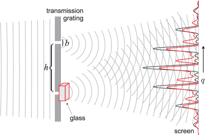
Figure 3: Graphic illustration of the Diffraction Grating problem setup with 2 slits. Incident light propagates through the slits – which along with the glass play the role of a phase function $\vec{\varphi}$ – and shines on the screen. The intensity $I_{DG}$ as a function of the position $q$ is then recorded, to become a position-based objective function.

The Diffraction Grating family of functions introduces a basic set of optical test-problems for Pareto optimization, scalable in dimension and subject to a collection of defining parameters for setting the Pareto front’s curvature.

Given a diffraction grating optical setup of $n$ slits, defined by the width of each slit $b$ and the space between adjacent slits $h$, and given a spatially uniform electromagnetic plane wave illuminating the slits with corresponding phases $\vec{\varphi}\in\left[0,2\pi\right]^{n}$, the intensity on a screen point in the Fraunhofer regime (i.e., far field) positioned at $q$ reads:

$$\begin{array}[]{l}\vskip 6.0pt plus 2.0pt minus 2.0pt\displaystyle I_{DG}\left(q,\vec{\varphi}\right)=\frac{1}{n^{2}}\textrm{sinc}^{2}\left(\frac{qb}{2}\right)\cdot\left|\sum_{k=0}^{n-1}\exp\left(iqhk\right)\cdot\exp\left(i\varphi_{k}\right)\right|^{2}\\ \displaystyle=\frac{1}{n^{2}}\textrm{sinc}^{2}\left(\frac{qb}{2}\right)\cdot\left\{n+2\cdot\sum_{k=0}^{n-1}\sum_{\ell>k}^{n-1}\cos\left[qh\left(\ell-k\right)+\Delta\varphi_{\ell k}\right]\right\},\end{array}$$ (15)

where $\vec{\varphi}=\left(\varphi_{0},\varphi_{1},\ldots,\varphi_{n-1}\right)^{T}$ and $\Delta\varphi_{\ell k}\equiv\varphi_{\ell}-\varphi_{k}$. Fig. 3 provides an illustration for the Diffraction Grating setup.

Given a set of $m$ competing points on the screen, described by a corresponding position vector $\vec{q}\in\mathbb{R}^{m}$, the $m$-objective Diffraction Grating problem to be Pareto optimized is defined as follows:

$$\vec{f}\left(\vec{q},\vec{\varphi}\right)=\begin{pmatrix}\displaystyle I_{DG}\left(q_{1},\vec{\varphi}\right)\\ \displaystyle I_{DG}\left(q_{2},\vec{\varphi}\right)\\ \vdots\\ \displaystyle I_{DG}\left(q_{m},\vec{\varphi}\right)\end{pmatrix}\longrightarrow\max$$ (16)

The shape of the Pareto front is determined by the positions of the points on the screen, and may furthermore be controlled by means of the parameters $b$ and $h$. This problem offers a rich variety of complexity levels, and can easily be extended to many different forms, such as multiple wavelengths, consideration of controllable amplitudes, nonlinear screens, 2-dimensional screens, etc.

Let us consider a setup with $b=1,~{}h=4$. The intensity values on the screen due to optical interferences follow a period, $T_{q}=\frac{2\pi}{h}$, and it is thus convenient to consider positions in terms of this period $T_{q}$. In our calculations we shall consider the maximization of the intensity at position zero, $q_{0}=0$, competing with the maximization of the intensity at the following positions: $q=\left\{0.1\cdot T_{q},~{}~{}0.25\cdot T_{q},~{}~{}0.5\cdot T_{q}\right\}$.

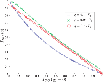
Figure 4: Approximate Pareto fronts, attained by the MO-CMA, of the competition between the intensity at $q_{0}=0$ to the intensity at each one of the positions $q=\left\{0.1\cdot T_{q},~{}~{}0.25\cdot T_{q},~{}~{}0.5\cdot T_{q}\right\}$ – formalized as bi-criteria problems following Eq. 16 with $n=10$ phase points. Given the fixed optical setup of the problem ($b=1,~{}h=4$), the positions of the competing points on the screen dictate the curvature of the Pareto front.

For illustration, approximate Pareto fronts (attained by the MO-CMA) of the competition between the intensity at $q_{0}=0$ to the intensity at each one of the positions $q=\left\{0.1\cdot T_{q},~{}~{}0.25\cdot T_{q},~{}~{}0.5\cdot T_{q}\right\}$ – formalized as bi-criteria problems following Eq. 16 with $n=10$ phase points – are depicted in Fig. 4. In addition, an approximate Pareto surface, obtained by the steady-state MO-CMA, presenting the competition between intensities of points positioned at $q_{0}=0$, $q_{1}=0.25\cdot T_{q}$, and $q_{2}=0.5\cdot T_{q}$ – formalized as a tri-objective problem (Eq. 16) with $n=10$ phase points – is depicted in Fig. 5.

In what follows, this study will focus on the bi-criteria case of $q_{1}=0.5\cdot T_{q}=\frac{\pi}{4}$, i.e.,

$$\begin{array}[]{l}\vskip 6.0pt plus 2.0pt minus 2.0pt\displaystyle f_{1}=I_{DG}\left(0,\vec{\varphi}\right)\longrightarrow\max\\ \displaystyle f_{2}=I_{DG}\left(\frac{\pi}{4},\vec{\varphi}\right)\longrightarrow\max\end{array}$$ (17)

This test-case has a linear Pareto front; see Appendix 0.A for the proof. Noise will be modeled here as with a QC phase function (Eq. 6), i.e., additive Gaussian variations on each phase coordinate:

$$\tilde{\vec{\varphi}}=\vec{\varphi}+\mathcal{N}\left(\vec{0},\epsilon_{S}^{2}\mathbf{I}\right).$$ (18)

Upon consideration of the noise propagation, the mean and the variance of the perceived fitness can be analytically derived (see Appendix 0.B). The mean may be presented in a compact form,

$$\begin{array}[]{l}\vskip 6.0pt plus 2.0pt minus 2.0pt\displaystyle\left<\tilde{f}_{i}\left(q_{i},\vec{\varphi}\right)\right>=\exp\left(-\epsilon_{S}^{2}\right)\cdot f_{i}\left(q_{i},\vec{\varphi}\right)+\\ \displaystyle+\textrm{sinc}^{2}\left(\frac{q_{i}b}{2}\right)\cdot\left(\frac{1-\exp\left(-\epsilon_{S}^{2}\right)}{n}\right),\end{array}$$ (19)

revealing both additive as well as multiplicative components to the disturbed objective function values. The variance, although possessing a closed analytical form, cannot be presented in a compact form, but rather in terms of explicit summation (Eqs. 50 and 53 are given in Appendix 0.B).

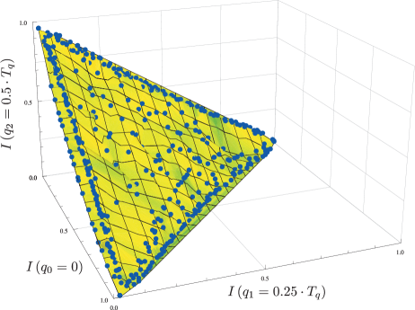
Figure 5: The tri-criteria Diffraction Grating problem: approximate Pareto surface, attained by the steady-state MO-CMA, of the competition between the intensities at $q_{0}=0$, $q_{1}=0.25\cdot T_{q}$, and $q_{2}=0.5\cdot T_{q}$ – following Eq. 16 with $n=10$ phase points.

4.2 Simulated Quantum Control System: Molecular Alignment

We consider the QC application to dynamic molecular alignment, which has been widely investigated in the past by means of noise-free simulations optimized by EAs (see, e.g., [47, 48]). The time evolution of heteromolecular diatomic alignment is quantum mechanically computed with the system starting either in the ground rotational level (i.e., at zero temperature), or in a Boltzmann distribution of initial states. The primary objective is maximization of molecular alignment, quantified by the cosine-squared observable, $\mathcal{O}_{1}=\cos^{2}(\theta)$, which considers the angle $\theta$ of the molecular axis with respect to the laser polarization axis. Fig. 6 provides an illustrative overview of the numerical process. This single-objective form was extended to a bi-criteria framework [49, 50], considering additionally the demand for low-intensity pulses, satisfied by minimizing second harmonic generation (SHG). The bi-criteria formulation is thus posed as obtaining the Pareto front given the following objectives:

$$\begin{array}[]{l}\vskip 6.0pt plus 2.0pt minus 2.0pt\displaystyle f_{1}=\left<\cos^{2}(\theta)\right>\longrightarrow\max\\ \displaystyle f_{2}=SHG\left(E(t)\right)=\int_{-\infty}^{\infty}|E(t)|^{4}dt\longrightarrow\min.\end{array}$$ (20)

For the explicit definition of the cosine-squared observable in $f_{1}$ we refer the reader to [51], while the electric field dependence in $f_{2}$ follows the formulation in Eq. 3. The values of both $f_{1}$ and $f_{2}$ are normalized to lie on the interval $[0,1]$. This bi-criteria molecular alignment problem was previously investigated only for the variant considering a distribution of initial rotational states [49, 50]. We shall study the problem variant starting in the ground state [48], which constitutes a simulation with a duration of 5sec per single evaluation. Even upon parallelization of the MO-CMA, we are still facing computationally expensive calculations, which will practically limit the employment of various strategies and in repeating runs to a certain degree, as will be described. We consider a discretization of $n=80$ points for the phase function.

We consider the introduction of noise to the phase pixels (Eq. 6), and incorporate it into the simulation. In order to evaluate the effect of this noise on the objective values $f_{1}$ and $f_{2}$, the Gaussian variation has to be explicitly propagated through the Fourier transform and the Schrödinger equation. Such an analytical evaluation is highly complex (especially for $f_{1}$), generally unknown, and exceeds the scope of this study.

It should be noted that the bi-criteria alignment problem was Pareto optimized by different variants of the NSGA-II [49] and of the SMS-EMOA [50], and will be introduced here to the MO-CMA algorithm.

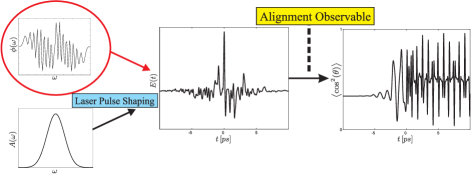
Figure 6: An overview of the numerical modeling of molecular alignment. The control function is the spectral phase (circled, top left), the amplitude function is fixed and approximated by a Gaussian (bottom left). The shaping process generates the electric field, $E(t)$ (center), corresponding to Eq. 3. The “Schrödinger Box” of the alignment observable represents the numerical calculation of the interaction between the electric field with the molecules, based on the specified quantum dynamics equations. The revival structure (right) is the observed simulated behavior of the molecules, upon which the yield value is based.

4.3 Experimental QC System I: Molecular Ion Generation

We consider the Pareto optimization of a QC experimental system in order to examine the conflict between two competing quantum mechanical observables. Total ion signal $\mathcal{J}_{Ion}$ resulting from multi-photon ionization of nitromethane with shaped, femtosecond pulses is examined with the goal of discovering a unique set of ionizing pulses. However, due to the high photon numbers ($\simeq 8$ photons at 800nm) required for single pulse ionization, ion generation is predominantly dictated by pulse intensity, which obfuscates sensitivity to detailed temporal control field structure. This inherent intensity dependence is removed by additionally considering $SHG^{\alpha}$, where $\alpha=2.5$ in the present circumstance, as shown later in the inset of Fig. 15 for the unshaped reference pulse. Towards this end, we seek to maximize the ion signal with low-intensity pulses, which naturally results in a conflict between $\mathcal{J}_{Ion}$ and $SHG^{\alpha}$:

$$\begin{array}[]{l}\vskip 6.0pt plus 2.0pt minus 2.0pt\displaystyle f_{1}=\mathcal{J}_{Ion}\longrightarrow\max\\ \displaystyle f_{2}=SHG^{\alpha}\longrightarrow\min.\end{array}$$ (21)

The search is carried out by means of $n=80$ independent phase pixels (see Eq. 4), while $\mathcal{J}_{Ion}$ is recorded with a mass spectrometer and SHG is monitored with a two-photon diode.

4.4 Experimental QC System II: Molecular Plasma Generation

As an extension of the molecular ion generation system, and as an application of the aforementioned Optimal Dynamic Discrimination concept, we consider here an equivalent conflict between competing plasma channels. Total free electron number $\mathcal{J}_{Plasma}$ resulting from multi-photon ionization of nitromethane with shaped, femtosecond pulses is diagnosed with radar scattering. Shaping is performed with the goal of discovering a unique set of ionizing pulses which discriminate against background plasma generation. Here, also, due to the high photon numbers required for single pulse ionization, electron generation is predominantly dictated by pulse intensity. Equivalently, we seek to explore the conflict between $\mathcal{J}_{Plasma}$ maximization and $SHG$ minimization, in an effort to discover unique, non-intensity dependent ionizing pulses:

$$\begin{array}[]{l}\vskip 6.0pt plus 2.0pt minus 2.0pt\displaystyle f_{1}=\mathcal{J}_{Plasma}\longrightarrow\max\\ \displaystyle f_{2}=SHG\longrightarrow\min.\end{array}$$ (22)

The search is carried out by means of $n=80$ independent phase pixels (see Eq. 4), while $\mathcal{J}_{Plasma}$ is recorded with a microwave transmitter/receiver and SHG is monitored with a two-photon diode.

The reader should keep in mind that despite some similarities in the two aforementioned laboratory systems – i.e., Molecular Ion Generation (Section 4.3) versus Molecular Plasma Generation (Section 4.4) – they possess very different experimental designs, and most importantly, they are subject to fundamentally different underlying physics. Table 1 summarizes the problems investigated in this study.

Table 1: Summary of Systems under Investigation

Simulations: Model Landscapes
Problem Name Formulation Dimensionality Noise Levels Multi-Sphere Eq. 11 $n=\left\{10,30,80\right\}$ $\epsilon_{x}^{2}=\left\{0.001,0.005,0.01,0.02,0.05\right\}$ Diffraction Grating Eqs. 15, 17 $n=\left\{10,30,80\right\}$ $\epsilon_{S}^{2}=\left\{0.001,0.005,0.01,0.02,0.05\right\}$
Real-World Simulator
Problem Name Description Dimensionality Noise Levels Molecular Alignment Eq. 20 $n=80$ $\epsilon_{S}^{2}=\left\{0.001,0.005,0.01,0.02,0.05\right\}$
Laboratory Experiments
Problem Name Description Dimensionality Measured Noise Level Total-Ion Generation Eq. 21 $n=80$ $\epsilon_{S}^{2}\approx 0.01$ Plasma Generation Eq. 22 $n=80$ $\epsilon_{S}^{2}\approx 0.01$

5 Practical Observations

We describe here our observations of the three frameworks specified in the previous section: Model landscapes, QC simulations, and QC experiments. Towards this end, we adhere to the structured reporting scheme suggested by Preuss [52], starting by posing the scientific question to answer. Each framework is treated by means of relevant methodologies, which depend upon the research question as well as upon the practical constraints (computational resources, experimental considerations, etc.). Section 5.1 focuses on the performance of the MO-CMA on the Multi-Sphere landscape subject to noise. Section 5.2 considers the performance of several EMOA on the Diffraction Grating problem. Section 5.3 reports on results of the simulated Molecular Alignment problem, and finally, sections 5.4 and 5.5 present laboratory results of the Molecular Ion Generation and Molecular Plasma Generation problems, respectively.

Pre-Experimental Planning. The MO-CMA code relies on the Shark Library release 2.2.1 [53]. The simulated systems are optimized by means of an extended MPI-based parallel implementation to the Shark code, while the laboratory employs an extended LabView version, which relies on Shark DLL’s. The default parameters are kept, with a total population size of either $\mu_{S}=\lambda_{S}=100$ search points for the simulations, or $\mu_{L}=\lambda_{L}=50$ search points in the laboratory. Random initialization of search points is carried out uniformly in the interval $\left[-10,10\right]^{n}$ for the Multi-Sphere cases, and in $\left[0,2\pi\right]^{n}$ otherwise. The initialization in the experimental systems also relies on seed search points, which were obtained in single-objective CMA-ES runs addressing a tailored ratio objective function.

The presentation of the results will include the archived perceived fronts attained by the MO-CMA for all frameworks under investigation. For the two simulated frameworks, we are in a privileged position to reevaluate archived solutions with noise-free objective functions, and thus we shall present also the ideal fronts, which are calculated a posteriori.

We would like to stress the fact that the perceived fronts, due to the elitist strategy in use, are expected to represent the tail of the disturbance distribution, as projected on the archived solutions. It is important to consider to what extent the attained perceived front may be reconstructed de facto given the archived solutions. Therefore, we will generate statistical samples of each archived solution, subject to the same noise conditions, and present additionally the nature of the obtained distributions. We consider this a direct indication of the usefulness of the archived solutions.

5.1 Preliminary: MO-CMA on the Multi-Sphere Landscape

Research Question. How does noise on the decision parameters affect the MO-CMA performance, if at all, and do any of the considered schemes of three parental re-evaluation scenarios (Section 3.2) handle noise better?

Performance Criteria. In order to assess the quality of the obtained Pareto fronts in the different noisy test-cases, we shall consider two performance criteria. Given the attained hypervolume indicator values, $V_{i}$ [54, 55] (also known as ’S-Metric’ [56] or ’Lebesgue Measure’ [57]), the first criterion is their relative deterioration with respect to the hypervolume of the Pareto front obtained in noise-free conditions, $V_{\epsilon_{x}=0}$. This criterion will be assessed numerically, for which we set up and test a corresponding quantifier:

$$\Delta_{V}^{(i)}=\frac{V_{\epsilon_{x}=0}-V_{i}}{V_{\epsilon_{x}=0}}.$$ (23)

The second criterion is the spatial distribution of the attained front, for which we set up and test a corresponding quantifier. In particular, given a final population of size $\mu$, $\left\{\vec{f}_{k}^{(i)}\right\}_{k=1}^{\mu}$, sorted by means of partial order, let us consider its $\chi^{2}$ value with respect to a reference noise-free population, $\left\{\vec{p}_{k}\right\}_{k=1}^{\mu}$, which toward this end represents a desired distribution of points along the front:

$$\Delta_{D}^{(i)}=\sum_{k=1}^{\mu}\frac{\|\vec{f}_{k}^{(i)}-\vec{p}_{k}\|^{2}}{\|\vec{p}_{k}\|}\sim\chi^{2}\left(\mu\right).$$ (24)

In essence, values given by Eqs. 23 and 24 reflect the degrees of deterioration in the hypervolume and the spatial diversity, respectively, with respect to the noise-free simulations.

5.1.1 Numerical Results

Setup. We consider here the numerical results of the various simulations on the Bi-Sphere model landscape. While the number of function evaluations per scheme varied, due to the parental re-evaluation procedure, the number of total iterations was fixed per search space dimensionality: $num_{iter}=\left\{10^{4},2\cdot 10^{4},5\cdot 10^{4}\right\}$ for $n=\left\{10,30,80\right\}$, respectively. Those values were set based on preliminary runs, in which the MO-CMA converged to a highly-satisfying front, with minimal error from the true Pareto front, and with a uniform distribution of points. For the hypervolume calculations, a reference point at $[2,2]$ is considered.

Experimentation/Visualization. We focus on presenting statistical analyses of specific test-cases, comparing the 3 different MO-CMA schemes. Overall, taking into account the a posteriori calculation, we shall have two sets of results per procedure. Fig. 8 depicts the statistical box-plots for $\Delta_{V}$ values of the Multi-Sphere landscape, taking into account only converged points in the box $[0,2]^{2}$ in the objective space, for three test-cases: $n=10$ with $\epsilon_{x}^{2}=0.05$ (top), $n=30$ with $\epsilon_{x}^{2}=0.02$ (middle), and $n=80$ with $\epsilon_{x}^{2}=0.01$ (bottom). Fig. 8 depicts the equivalent box-plots for the $\Delta_{D}$ calculations (considering all 30 runs per case).

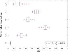
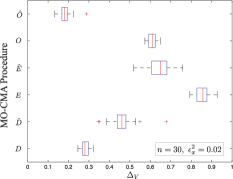
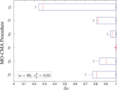
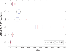
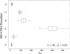
Figure 7: Box-plots of $\Delta_{V}$ values (Eq. 23) over all converged Multi-Sphere runs, of three test-cases: $n=10$ with $\epsilon_{x}^{2}=0.05$ [top], $n=30$ with $\epsilon_{x}^{2}=0.02$ [middle], and $n=80$ with $\epsilon_{x}^{2}=0.01$ [bottom]. The perceived fronts of the three optimization procedures, corresponding to the three parental re-evaluation scenarios (Section 3.2), are noted as $\left\{D,~{}E,~{}O\right\}$. The ideal fronts (noise-free evaluation of the Pareto sets) are noted as $\left\{\hat{D},~{}\hat{E},~{}\hat{O}\right\}$. Each case consists of 30 runs.

Figure 8: Box-plots of $\Delta_{D}$ values (Eq. 24) over all converged Multi-Sphere runs, of three test-cases: $n=10$ with $\epsilon_{x}^{2}=0.05$ [top], $n=30$ with $\epsilon_{x}^{2}=0.02$ [middle], and $n=80$ with $\epsilon_{x}^{2}=0.01$ [bottom]. The perceived fronts of the three optimization procedures, corresponding to the three parental re-evaluation scenarios (Section 3.2), are noted as $\left\{D,~{}E,~{}O\right\}$. The ideal fronts (noise-free evaluation of the Pareto sets) are noted as $\left\{\hat{D},~{}\hat{E},~{}\hat{O}\right\}$. Each case consists of 30 runs.

5.1.2 Discussion

While the perceived fronts given as output by the MO-CMA provide fair Pareto approximations, with some expected error due to the presence of noise, an examination of the actual archived solutions reveals an entirely different picture. When exposed to noise on the decision parameters, the default MO-CMA is observed to lack population diversity in the objective space for all search space dimensions under investigation. This effect becomes evident upon the a posteriori noise-free evaluation of the archived solutions: the outcome is several clustered points along the perceived front, as depicted in Fig. 9. The lack of diversity continually worsens as the expected disturbance increases, i.e., higher noise strength and higher dimensionality lead to increased clustering. Fig. 8 depicts box-plots for the $\Delta_{D}$ values of 3 Bi-Sphere test-cases. While the raw $\Delta_{D}$ values do not reflect the degree of discrepancy by themselves, it is important to consider those values with respect to the perceived front of the default MO-CMA, which typically obtains a fair approximation to the true front given the disturbance. This effect may also be observed in Fig. 8, when noticing the considerable counter-intuitive differences in the $\Delta_{V}$ values between the default MO-CMA (’$D$’) and its a posteriori noise-free evaluation (’$\hat{D}$’).

The proposed explanation for the observed lack of diversity is the following. During the run, search points which lead in the progress towards the Pareto front generate offspring by means of Gaussian sampling (Eq. 9). Offspring with good positions with respect to the front, especially whose disturbed fitness values lie along the currently progressing front, are selected, and their decision parameters are archived. While the perceived offspring’s point in the objective space may represent a promising coordinate with respect to ranked domination as well as to hypervolume contribution, its pre-image in the decision space is merely a small deviation from the original parent. In practice, leading individuals take-over the population, since generating offspring by means of small mutations in combination with the noise disturbance is sufficient to span a fair distribution along the Pareto front. This statement was numerically assessed by explicitly calculating the expected distribution with the analytical forms of Eqs. 13 and 14, and it was furthermore corroborated with the sampling of the actual archived Pareto optimal set of an MO-CMA run. The aforementioned calculations are depicted in Fig. 9, which provides a clear picture – the obtained clusters are the minimal configuration of points for sampling the entire Pareto front with the current noise level, and moreover, the perceived front can indeed be reconstructed by elitist selection of the attained statistical sample. It is also evident from further calculations that the number of clusters increases with the reduction of noise disturbance, as expected from Eqs. 13 and 14. This clustering effect may be considered as a multi-objective generalization to the systematic overvaluation effect, as discussed by Arnold and Beyer for the single-objective case in [44]. We thus claim that fitness disturbance in multi-objective optimization is responsible for the low objective space diversity in the archiving mechanism of the MO-CMA.

As a second routine employed, parental re-evaluation every generation clearly hampered the performance of the default MO-CMA. The attained solutions constitute worst quality sets, when compared to the default procedure, for all the different test-cases under investigation. This poor performance may be clearly observed in Figs. 8 and 8 when considering ’$E$’ / ’$\hat{E}$’. The explanation for this behavior is a stochastic disturbance to the archiving mechanism, which has a direct negative impact on the consistency of the selection phase.

The third routine, MO-CMA with occasional parental re-evaluation (every 10 generations), seems empirically to be the best solution for the systematic disturbance problem. While low population diversity, as assessed with $\Delta_{D}$ values, is still observed upon the a posteriori noise-free evaluation of the archived solutions, the attained clusters are bigger in size, and closer to the true Pareto front. Essentially, the archived solutions of this procedure are of the highest quality when reconstructed a posteriori in comparison to the other procedures (see ’$O$’ / ’$\hat{O}$’ in Figs. 8 and 8). The perceived Pareto front is typically not as good as the one attained by the default MO-CMA, but unlike the default procedure, the a posteriori noise-free evaluation yields a better Pareto front in comparison to its perceived front, and especially better than the post-default front. This effect is also visually apparent when exploring the box-plots of both quantifiers and noting the inversion of roles: while ’$D$’ is always of higher quality than ’$\hat{D}$’, ’$O$’ is of lower quality than ’$\hat{O}$’. We conclude that in line with the single-objective scenario, occasional parental fitness re-evaluation seems to be superior with respect to no re-evaluation at all and to re-evaluation in every generation.

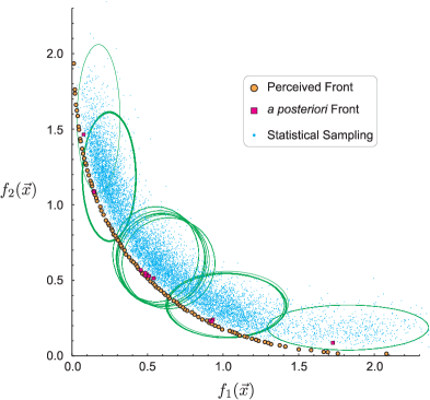
Figure 9: Statistical sampling of the Pareto set attained by the MO-CMA on the Multi-Sphere with $n=10$ at $\epsilon_{x}^{2}=0.01$. The perceived Pareto front constitutes an excellent approximation to the true front, and the a posteriori noise-free evaluation of its pre-images yields clusters along the front, whose sampling subject to the same noise level yields the depicted cloud of points. The ellipses represent the disturbance distributions, centered about the mean with twice the standard deviations as axis, based upon the analytical forms of the perceived fitness in Eqs. 13 and 14. It is clear from these results that the clusters are the minimal configuration of points for sampling the entire Pareto front, subject to elitism, with the current noise level.

5.1.3 Reference Algorithms

We considered additional standard EMOA as reference methods to the MO-CMA, in order to observe their behavior on the Multi-Sphere model landscape, subject to the current modeling of noise. We carried out simulations on similar test-cases with the NSGA-II [8] as well as with the SMS-EMOA [58]. We employ Deb’s operators and his defaults settings for the NSGA-II. Regarding the SMS-EMOA, we follow the settings described at [SMS-EMOA_Journal]. The population sizes are similar to those employed by the MO-CMA. These settings hold for the application of both NSGA-II and SMS-EMOA throughout the entire study. Typical runs of both algorithms on the case of $n=10$ with $\epsilon_{x}^{2}=0.01$ are depicted in Fig. 10, presenting the perceived fronts versus the a posteriori noise-free evaluation of the attained Pareto optimal sets.

Figure 10: Typical runs of the reference EMOA on the noisy Multi-Sphere case of $n=10$ with $\epsilon_{x}^{2}=0.01$: [LEFT (a)] NSGA-II versus [RIGHT (b)] SMS-EMOA. The figures depict the perceived fronts, the a posteriori noise-free evaluation of the Pareto optimal sets, and the analytical Pareto front (Eq. 12).

The NSGA-II attained a perceived Pareto front which constitutes a good approximation to the true front, and at the same time, the noise-free reconstruction of the Pareto optimal set provides a reasonable front. The SMS-EMOA, on the other hand, attained a perceived Pareto front which offers an excellent approximation to the true front, and upon the noise-free re-evaluation of the Pareto optimal set the reconstructed front is observed to lose its diversity to some extent. It should be stressed that the absolute ’clustering effect’ within the archiving mechanism, which was typical of the MO-CMA, was not observed for these reference algorithms. This might reflect the difference between an algorithm which is clearly designed for learning distributions (i.e., employing statistical learning), such as the MO-CMA, versus EMOA with traditional evolutionary core mechanisms, which evidently operate in a naïve way. Overall, in terms of the capacity to reconstruct Pareto information out of the archived solutions, SMS-EMOA seems to perform best on the Multi-Sphere noisy model landscape. A more comprehensive performance comparison between these three EMOA will be carried out in the following section with regard to the Diffraction Grating model landscape.

5.1.4 Noisy Tri-Sphere Simulations

Finally, we tested the behavior of the MO-CMA on the Tri-Sphere case (Eq. 11 with $m=3$). Toward this end, we employed a steady-state implementation which reduces the extensive complexity of the hypervolume calculations. We provide here a brief qualitative description of our observations. The MO-CMA obtained a good approximate Pareto surface for the noise-free problem. Upon consideration of systematic noise on the decision parameters, as done in the Bi-Sphere case, the diversity loss effect in the archiving mechanism of the decision space is not observed to be significant any longer, even at high noise levels of, e.g., $\epsilon_{x}^{2}=0.05$. We propose the following explanation for this observation: given the selection mechanism of the MO-CMA, treatment of an additional objective reduces the selection pressure. Lower pressure may thus reduce the probability of take-over, which was our understanding of the mechanism for the ’clustering effect’.

5.2 Diffraction Grating: Extensive Performance Comparison

Rather than considering the individual performances of the 3 MO-CMA schemes, we present a comprehensive performance comparison between the default MO-CMA, SMS-EMOA, and NSGA-II on the Diffraction Grating problem in several dimensions and at various noise levels. As a secondary research question, we aim at reporting on the MO-CMA behavior on this problem.

Let us begin by qualitatively describing the MO-CMA behavior on this search problem, in light of the observation reported in Section 5.1. Fig. 11 depicts typical results of the MO-CMA on two variants of the Diffraction Grating problem with $n=10$ phase points at two noise levels. Equivalent to Fig. 9, the Pareto sets are reconstructed a posteriori in noise-free evaluations, then statistically sampled at the same noise levels of the evolutionary run, and compared to the perceived Pareto fronts, given as output by the algorithm. As a reference, the ellipses representing the noise distribution are plotted, according to Eq. 19 (mean) and Eq. 50-53 (variance; see Appendix 0.B). It is straightforward to observe the ’clustering effect’ in the archiving mechanism, similar to the one occurring in the Multi-Sphere case.

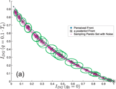
Figure 11: Statistical sampling of the Pareto optimal sets attained by the MO-CMA for two variants of the Diffraction Grating problem with $n=10$ phase points. Equivalent to Fig. 9, the Pareto sets are reconstructed by means of noise-free evaluation, and compared to their statistical sampling at the noise level of the evolutionary run, as well as to the perceived Pareto fronts, given as output by the algorithm. As a reference, the noise distributions are depicted according to the analytical results of Eq. 19 (mean) and Eqs. 50 and 53 (variance; see Appendix 0.B). [LEFT, (a)] Maximization of $I_{DG}(q_{0}=0)$ versus $I_{DG}(q=0.1\cdot T_{q})$ at $\epsilon_{x}^{2}=0.01$. [RIGHT, (b)] Maximization of $I_{DG}(q_{0}=0)$ versus $I_{DG}(q=0.25\cdot T_{q})$ at $\epsilon_{x}^{2}=0.05$.

5.2.1 Numerical Results

Setup. We consider here simulations on a specific case of the Diffraction Grating problem (Eqs. 15 and 17 set up with $b=1,~{}h=4$), in search space dimensions of $n=\left\{10,~{}30,~{}80\right\}$, and at noise levels given by Eq. 10. We fix the total number of function evaluations per search space dimensionality: $num_{evals}=\left\{10^{6},2\cdot 10^{6},5\cdot 10^{6}\right\}$ for $n=\left\{10,30,80\right\}$, respectively. For the hypervolume calculations, a reference point at $[0,0]$ is considered.

Experimentation/Visualization. Next, we shall consider the performance of the three EMOA on the given Pareto problems, considering the hypervolume indicator as the performance criterion. Based on the analytical expressions of the Pareto front for this problem, given in Appendix 0.A, the hypervolume of the true front is $\mho^{*}=0.47482$. Table 2 presents the mean and standard-deviations of the hypervolume calculations over 30 runs of the attained Pareto fronts for the various test-cases. The table contains the hypervolume values for the perceived fronts, as well as for the noise-free a posteriori fronts. Table 3 provides the Mann-Whitney U-test calculations for the pairwise algorithm comparisons corresponding to the test-cases of Table 2.

Table 2: Hypervolume Calculations: the Grating Diffraction Landscape ($b=1$, $h=4$; $q_{0}=0$, $q=0.5\cdot T_{q}$; $n=\left\{10,30,80\right\}$). Mean and standard-deviations over 30 runs, considering a reference point at $(0,0)$.Based on the analytical expressions of the Pareto front for this problem, given in Appendix 0.A, the hypervolume of the true front is $\mho^{*}=0.47482$.

n=10
Noise MO-CMA-ES SMS-EMOA NSGA-II Strength perceived a posteriori perceived a posteriori perceived a posteriori $\epsilon_{S}^{2}=0$ 0.47476$\pm$0.0001 0.47476$\pm$0.0001 0.47443$\pm$0.0004 0.47443$\pm$0.0004 0.31258$\pm$0.0669 0.31258$\pm$0.0669 $\epsilon_{S}^{2}=0.001$ 0.47420$\pm$0.0001 0.47420 $\pm$ 0.0004 0.47339$\pm$0.0016 0.47219$\pm$0.0025 0.39245$\pm$0.0472 0.37274$\pm$0.0575 $\epsilon_{S}^{2}=0.005$ 0.47398$\pm$0.0002 0.47158$\pm$0.0031 0.47128$\pm$0.0039 0.46473$\pm$0.0082 0.35833$\pm$0.0584 0.34559$\pm$0.0638 $\epsilon_{S}^{2}=0.01$ 0.47362$\pm$0.0007 0.46682$\pm$0.0069 0.46972$\pm$0.0042 0.45733$\pm$0.0116 0.39245$\pm$0.0472 0.37274$\pm$0.0575 $\epsilon_{S}^{2}=0.02$ 0.47316$\pm$0.0006 0.46285$\pm$0.0091 0.47018$\pm$0.0024 0.45215$\pm$0.0104 0.40789$\pm$0.0357 0.37518$\pm$0.0504 $\epsilon_{S}^{2}=0.05$ 0.47168$\pm$0.0008 0.44705$\pm$0.0158 0.46488$\pm$0.0049 0.42055$\pm$0.0259 0.42755$\pm$0.0317 0.38169$\pm$0.0433
n=30
Noise MO-CMA-ES SMS-EMOA NSGA-II Strength perceived a posteriori perceived a posteriori perceived a posteriori $\epsilon_{S}^{2}=0$ 0.43685$\pm$0.0448 0.43685$\pm$0.0448 0.46864$\pm$0.0034 0.46864$\pm$0.0034 0.24917$\pm$0.0291 0.24917$\pm$0.0291 $\epsilon_{S}^{2}=0.001$ 0.40817$\pm$0.0622 0.40395$\pm$0.0647 0.46080$\pm$0.0123 0.45902$\pm$0.0134 0.30131$\pm$0.0347 0.28343$\pm$0.0372 $\epsilon_{S}^{2}=0.005$ 0.42474$\pm$0.0435 0.41412$\pm$0.0482 0.44955$\pm$0.0117 0.44130$\pm$0.0152 0.28015$\pm$0.0428 0.26685$\pm$0.0435 $\epsilon_{S}^{2}=0.01$ 0.40719$\pm$0.0529 0.38921$\pm$0.059 0.44051$\pm$0.0128 0.42709$\pm$0.0177 0.30131$\pm$0.0347 0.28343$\pm$0.0372 $\epsilon_{S}^{2}=0.02$ 0.41905$\pm$0.0435 0.39627$\pm$0.0531 0.42513$\pm$0.0207 0.39920$\pm$0.0316 0.32415$\pm$0.0362 0.29869$\pm$0.0377 $\epsilon_{S}^{2}=0.05$ 0.40997$\pm$0.0392 0.37579$\pm$0.0466 0.41614$\pm$0.0139 0.37495$\pm$0.0240 0.35147$\pm$0.0252 0.31039$\pm$0.0335
n=80
Noise MO-CMA-ES SMS-EMOA NSGA-II Strength perceived a posteriori perceived a posteriori perceived a posteriori $\epsilon_{S}^{2}=0$ 0.35875$\pm$0.0515 0.35875$\pm$0.0515 0.45796$\pm$0.0104 0.45796$\pm$0.0104 0.20782$\pm$0.0440 0.20782$\pm$0.0440 $\epsilon_{S}^{2}=0.001$ 0.27607$\pm$0.0451 0.27123$\pm$0.0452 0.44408$\pm$0.0146 0.44289$\pm$0.0152 0.23867$\pm$0.0388 0.22717$\pm$0.0398 $\epsilon_{S}^{2}=0.005$ 0.26278$\pm$0.0458 0.25099$\pm$0.0460 0.42345$\pm$0.0146 0.41800$\pm$0.0170 0.24902$\pm$0.0343 0.24310$\pm$0.0347 $\epsilon_{S}^{2}=0.01$ 0.25462$\pm$0.0327 0.23735$\pm$0.0329 0.40138$\pm$0.0198 0.39219$\pm$0.0222 0.23867$\pm$0.0388 0.22717$\pm$0.0398 $\epsilon_{S}^{2}=0.02$ 0.25478$\pm$0.0482 0.23163$\pm$0.0463 0.38329$\pm$0.0245 0.36870$\pm$0.0292 0.25967$\pm$0.0350 0.24304$\pm$0.0378 $\epsilon_{S}^{2}=0.05$ 0.22611$\pm$0.0358 0.19538$\pm$0.0369 0.34807$\pm$0.0250 0.32100$\pm$0.0308 0.28492$\pm$0.0333 0.25748$\pm$0.0386

Table 3: Mann-Whitney U-Test Calculations: the Grating Diffraction Problem ($b=1$, $h=4$; $q_{0}=0$, $q=0.5\cdot T_{q}$; $n=\left\{10,30,80\right\}$). A comparison is drawn from the numerical results of the 3 algorithms in the various test-cases, considering a null hypothesis $H_{0}$ stating that there is no performance difference in terms of the attained hypervolume, versus a hypothesis $H_{1}$ stating that two algorithms have significantly different performance. Accordingly, a table symbol of $\pm$ indicates a rejection of the null hypothesis at the 5% significance level, whereas a symbol of $\approx$ indicates a failure to reject the null hypothesis at the 5% significance level. $+$ refers to a statistically significant outperformance of the left-side algorithm over the right-side algorithm, and $-$ indicates the reverse scenario.

n=10
Noise perceived a posteriori Strength CMA/SMS CMA/NSGA-II SMS/NSGA-II CMA/SMS CMA/NSGA-II SMS/NSGA-II $\epsilon_{S}^{2}=0$ $+$ $+$ $+$ $+$ $+$ $+$ $\epsilon_{S}^{2}=0.001$ $\approx$ $+$ $+$ $+$ $+$ $+$ $\epsilon_{S}^{2}=0.005$ $+$ $+$ $+$ $+$ $+$ $+$ $\epsilon_{S}^{2}=0.01$ $+$ $+$ $+$ $+$ $+$ $+$ $\epsilon_{S}^{2}=0.02$ $+$ $+$ $+$ $+$ $+$ $+$ $\epsilon_{S}^{2}=0.05$ $+$ $+$ $+$ $+$ $+$ $+$
n=30
Noise perceived a posteriori Strength CMA/SMS CMA/NSGA-II SMS/NSGA-II CMA/SMS CMA/NSGA-II SMS/NSGA-II $\epsilon_{S}^{2}=0$ $\approx$ $+$ $+$ $\approx$ $+$ $+$ $\epsilon_{S}^{2}=0.001$ $-$ $+$ $+$ $-$ $+$ $+$ $\epsilon_{S}^{2}=0.005$ $\approx$ $+$ $+$ $\approx$ $+$ $+$ $\epsilon_{S}^{2}=0.01$ $-$ $+$ $+$ $-$ $+$ $+$ $\epsilon_{S}^{2}=0.02$ $\approx$ $+$ $+$ $\approx$ $+$ $+$ $\epsilon_{S}^{2}=0.05$ $\approx$ $+$ $+$ $\approx$ $+$ $+$
n=80
Noise perceived a posteriori Strength CMA/SMS CMA/NSGA-II SMS/NSGA-II CMA/SMS CMA/NSGA-II SMS/NSGA-II $\epsilon_{S}^{2}=0$ $-$ $+$ $+$ $-$ $+$ $+$ $\epsilon_{S}^{2}=0.001$ $-$ $+$ $+$ $-$ $+$ $+$ $\epsilon_{S}^{2}=0.005$ $-$ $\approx$ $+$ $-$ $\approx$ $+$ $\epsilon_{S}^{2}=0.01$ $-$ $\approx$ $+$ $-$ $\approx$ $+$ $\epsilon_{S}^{2}=0.02$ $-$ $\approx$ $+$ $-$ $\approx$ $+$ $\epsilon_{S}^{2}=0.05$ $-$ $-$ $+$ $-$ $-$ $+$

5.2.2 Discussion

Given the numerical results in Table 2 and the statistical tests in Table 3, we suggest the following observation: while the MO-CMA achieves superior hypervolume values on the 10-dimensional case, there is no clear winner on the 30-dimensional case (see U-tests), and finally, the SMS-EMOA is the winner on the 80-dimensional cases. In the vast majority of the cases, the NSGA-II is outperformed by its competitors.

We speculate whether the poor performance of the MO-CMA in the high-dimensional cases in comparison to the SMS-EMOA is due to an insufficient budget of function evaluations. Upon granting the MO-CMA additional function evaluations for the high-dimensional cases this speculation is indeed corroborated. We carried out $30$ independent runs for the noise-free test cases of $n=30$ and $n=80$, with $10$ times the original budget of function evaluations, i.e., with $2\cdot 10^{7}$ and $5\cdot 10^{7}$ function evaluations, respectively. For the $n=30$ test-case the MO-CMA obtained a mean hypervolume value of $0.47465$, whereas for the $n=80$ test-case it obtained a mean hypervolume value of $0.46089$. Fig. 12 depicts statistical box-plots describing the miscellaneous runs granting the MO-CMA additional function evaluations for the high-dimensional noise-free cases, presenting the attained hypervolume values at specific milestones along the runs. As stated earlier, it is indeed shown that the MO-CMA is slower than the SMS-EMOA for those problems, but it is capable of eventually converging to a good approximate front, given sufficient function evaluations.

The empirically observed slow progress rate may be attributed to the self-adaptation mechanism which is typically responsible for the relatively long learning period of the CMA-ES when compared to other strategies, e.g., ES with fewer strategy parameters [59, 60]. Overall, it seems that employing the strong search-engine of the CMA does not pay off on the Diffraction Grating problem upon consideration of the reduced convergence speed in comparison to the SMS-EMOA.

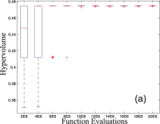
Figure 12: Granting the MO-CMA additional function evaluations for the noise-free Diffraction Grating problem. Statistical box-plots of 30 independent runs, presenting the attained hypervolume values at specific milestones along the run, with up to 10 times the original budget of function evaluations. [LEFT, (a)] $n=30$, where the algorithm obtains the maximally attainable hypervolume in all runs, without exception, after $2\cdot 10^{7}$ function evaluations; [RIGHT, (b)] $n=80$, where the majority of the runs obtain the maximally attainable hypervolume after $5\cdot 10^{7}$ function evaluations.

5.3 Molecular Alignment Simulations

We consider the detailed effect of pixel noise on the quantum observables and the overall MO-CMA performance.

Performance Assessment. In the context of molecular alignment (Eq. 20), $f_{1}$ is of particular interest, and thus is considered as the primary objective. The maximally attainable theoretical upper bound that can be supported by the utilized rotational states used here was found to be 0.9863 [48], but the best known single-objective $f_{1}$ yield within the current bandwidth discovered by an ES was reported to be 0.962 [48], with a corresponding $f_{2}$ value of 0.154. The nature of the conflict between $f_{1}$ to $f_{2}$ is generally unknown, and we shall use our noise-free runs as a reference Pareto front for the runs on noisy systems.

Setup. Due to computational limitations, we set a limit of 10 runs per test-case. Preliminary runs of MO-CMA, SMS-EMOA and NSGA-II on the noise-free simulation are carried out as an introductory comparison. Furthermore, we will take into account systems with noisy controls subject to the noise strength values of Eq. 10. Each run is limited to 1000 iterations.

Figure 13: Attained Pareto fronts on the noise-free molecular alignment simulation of 4 EMOA routines: MO-CMA with ’plain’ parametrization (decision variables are directly addressed as phase points), MO-CMA with Hermite parametrization (decision variables correspond to coefficients of the first 40 Hermite polynomials, spanning altogether the phase), SMS-EMOA, and NSGA-II. Each front is reconstructed of 10 runs per routine.

Preliminary: EMOA Noise-Free Comparison. The noise-free runs yielded disconnected local Pareto fronts, which offered limited coverage of the objective space per run. This may suggest that the search space is broken into separate regions, partitioned by barriers, possibly due to the inherent constraints on the system, e.g., the bandwidth, the discretization, etc. We reconstructed a single Pareto front from these runs, referred to here as the best known Pareto front. The shape of the attained front indicates that the conflict is rather soft, as high $f_{1}$ values may be obtained while keeping $f_{2}$ values extremely low. There seems to be no considerable pay-off in $f_{1}$ when unleashing $f_{2}$. Furthermore, from a practical perspective one may argue that this conflict is irrelevant, as the observed $f_{2}$ values are sufficiently low. It should also be noted that $f_{1}$ values of $\approx$0.96 could not be attained in these runs; the best obtained value was $f_{1}^{*}=0.947$, corresponding to $f_{2}^{*}=0.165$. This observation may be linked to previous reports on the single-objective CMA-ES applied to this problem [48], investigating its performance in maximizing $f_{1}$ subject to various parametrizations. In particular, the so-called ’plain’ parametrization, where the decision variables correspond to the phase function pixels, was observed to be inferior in comparison to specific polynomial-based configurations, where the decision variables played the role of coefficients of complete-basis functions. In [48], following an empirical comparison, the Hermite polynomials were reported to perform best. Here, we carried out additional calculations, employing the Hermite parametrization, in order to assess the latter observation. The results, which are depicted in Fig. 13, generalize the observation reported in [48] into the bi-criteria picture, confirming that the MO-CMA is capable of attaining $f_{1}$ values of $\approx$0.96 when special configurations are in use. Moreover, it confirms that the inherent advantage of the Hermite parametrization in terms of $f_{1}$ values translates into a trade-off with slightly higher $f_{2}$ values. Concerning the competing SMS-EMOA and NSGA-II algorithms, it is clearly observed that they present inferior performance, especially with respect to the coverage of $f_{1}$ values. In total, their results are disappointing, but at the same time are in some consistency with previous observations on a different variant of this problem (see, e.g., [49]).

Observation: MO-CMA on Noisy Systems. In what follows, we consider the MO-CMA alone on the noisy alignment problem. When subject to noise, the MO-CMA seems to perform well, especially with its default procedure, in obtaining fair Pareto fronts, in comparison to the noise-free simulations. As in the noise-free case, the attained fronts were typically broken, and we reconstructed them into a single front for their presentation. In some cases, the perceived Pareto fronts of the noisy system dominated the best known front, and the a posteriori noise-free evaluation of the archived phase functions introduced a local improvement to the best known front. This is an example of a scenario in which fitness overvaluation has the potential to enhance the search. However, the reproduction of the Pareto front by evaluating the Pareto optimal set typically failed, suggesting that decision space information was lost, as was observed on the model landscape. Fig. 14[a] depicts the attained front of the default MO-CMA procedure in a noisy system of $\epsilon_{S}^{2}=0.01$. The plot contains the reconstructed Pareto front of 10 runs, the best known front, the a posteriori noise-free evaluation of the Pareto optimal set, as well as the noisy sampling of the Pareto optimal set. Close examination of the a posteriori sampled data and their grouping towards the perceived front reveals interesting insight into the noise propagation through the two objective functions (Fig. 14[b]). It is evident that noisy sampling of a phase function corresponding to a point on the perceived front results in an elliptic cloud of points, whose elitist outliers constitute the points of the perceived front, as in the model landscapes (see, e.g., Fig. 9). Also, it is clear that these clouds have a dominant horizontal axis in the current scaling. This observation suggests that the alignment observable ($f_{1}$) is sensitive to noise, unlike SHG ($f_{2}$), which is hardly affected by it at the current noise level. Moreover, the shape of these clouds seems to be dependent upon the two objective values through a multiplicative relation: points with low $f_{1}$ values possess a longer horizontal axis and a shorter vertical axis in comparison to points with higher $f_{1}$ values.

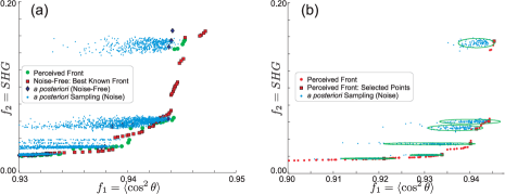
Figure 14: The attained reconstructed Pareto front of the default MO-CMA on the noisy alignment simulation with $\epsilon_{S}^{2}=0.01$. [LEFT (a)] The reconstructed perceived front of 10 runs, the best known front, the a posteriori noise-free evaluation of the Pareto optimal set, and the a posteriori noisy sampling of the Pareto optimal set. [RIGHT (b)] Statistical examination of the a posteriori sampling of selected points of the Pareto optimal set. Each sampling set comprises 100 evaluations at the noise level of $\epsilon_{S}^{2}=0.01$. The ellipses represent the disturbance distributions, centered about the mean with twice the standard deviations as axes, based upon statistics of the attained data. As in the model landscapes (see, e.g., Fig. 9), the perceived front constitutes an elitist selection of these distributions. The reader should mind the different horizontal scaling of the two panels.

It should be noted that the simulations at higher noise levels obtained reasonable Pareto fronts in comparison to the noise-free best known front, but their reproduction by means of evaluation with the attained Pareto optimal set failed, as found on the Multi-Sphere model landscape. The simulations also revealed that the two procedures with additional parental fitness re-evaluations produced Pareto fronts of low quality, as they were typically dominated by the default MO-CMA procedure. In some cases, however, it is evident that local a posteriori Pareto fronts of the procedure with occasional parental re-evaluation locally dominated the equivalent fronts of the default procedure. Overall, there is no clear superior procedure in this test-case.

5.4 Laboratory Experiment I: Molecular Ion Generation

An experimental Pareto front for the molecular ion generation system is depicted in Fig. 15. The shape of the front has been assessed with high confidence, based on numerous runs of the single-objective $\left(\mu,\lambda\right)$-CMA-ES on the corresponding tailored ratio objective function, i.e., $\frac{\mathcal{J}_{Ion}}{SHG^{\alpha}}$. We therefore conclude that the MO-CMA obtained a perceived Pareto front consistent with the repeated aforementioned single-objective optimization results, but nevertheless, its reconstruction by means of the attained Pareto set was not successful, as observed with both the Multi-Sphere and the molecular alignment problems. It is evident in Fig. 15 that while the perceived Pareto front dominates the unshaped control reference front, the mean values of the a posteriori sampling of the Pareto set produces a dramatically worse front, which is Pareto indifferent to the reference front. In addition, the attractive knee point (roughly located around coordinate (0.425,0.2)) could not be reconstructed, and its information was practically lost. Upon consideration of the experimental data, the perceived point appears to be an experimental outlier, which dominated a converging local Pareto front in that domain and contributed to its loss. However, it is crucial to note that this specific knee area represents a real domain of solutions which has been identified in repeated occasions, whose Pareto coverage is much needed. Repeating runs by means of alternative strategies introduced an experimental overhead, and therefore was not carried out. The second QCE system, Molecular Plasma Generation, possesses higher experimental stability, granted by the different experimental design. It has therefore been targeted as a platform for testing the re-evaluation approach and thus to address the issues revealed with the current experimental system. Moreover, it allowed for a comparison between various strategies, as will be described in the following section.

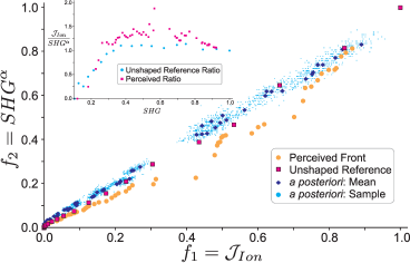
Figure 15: Experimental Pareto front of the default MO-CMA on the total ionization $\mathcal{J}_{Ion}$ versus SHG problem. The figure depicts the perceived front of a single experiment, the reference front of the intensity based non-shaped pulse, as well as a sampling of the Pareto set. Inset: single-objective ratio picture.

5.5 Laboratory Experiment II: Molecular Plasma Generation

Taking advantage of the experimental stability of this system, we carried out a Pareto optimization campaign by means of the EMOA considered in the current study. In particular, we compared the experimental performance of the MO-CMA (default and with occasional parental re-evaluation), to the NSGA-II and the SMS-EMOA. The observation here is clear, as well as consistent with the previous observations on the other systems: The default MO-CMA produced highly-satisfying perceived fronts, but suffered from an inability to reproduce them upon the termination of the runs. The NSGA-II, on the other hand, performed poorly, and failed to obtain good approximations to the Pareto front. The remaining strategies, MO-CMA with occasional re-evaluation and the SMS-EMOA, both performed well – the attained approximate fronts were satisfying, and their post-reproduction was successful. Fig. 16 presents successful runs of both strategies, depicting the perceived fronts, their reproduction, and the unshaped reference fronts (measured upon scanning the amplitude of an unshaped pulse). Since the latter represents a trivial reference to pulse shaping, and especially to any QC optimization scheme, we argue that the QC optimization pay-off in the multi-objective case may be assessed by the calculation of the hypervolume ratio between the attained front to the unshaped reference front. Overall, the MO-CMA with occasional parental re-evaluation performed best, introducing a hypervolume improvement of 24.5% with respect to the unshaped reference. The SMS-EMOA, on the other hand, introduced an insignificant improvement of merely 3%, due to bad coverage. The success of the occasional re-evaluation scheme within the MO-CMA proved to be especially beneficial in this case, and thus constitutes an experimental corroboration to the conclusions drawn on noisy model landscapes (see Section 5.1). Fig. 17 depicts the evolving hypervolume pay-off of the MO-CMA population – presented as the ratio between the raw MO-CMA hypervolume to the hypervolume of the unshaped reference front – corresponding to the run presented in Fig. 16[(a)]. For the hypervolume calculations, a reference point at $[0,1]$ is considered. The initial high values of the ratio around 0.9 are a consequence of planting seed solutions in the initial population. It can be clearly observed that the occasional re-evaluation (every 10 generations) introduces corrections to fitness disturbances of the parental population that translate into hypervolume declines. In particular, note the dramatic decline following the re-evaluation of generation 30 – had not this correction occurred, the parental population would have been contaminated by extreme outliers and the run would have been affected accordingly. At the same time, the re-evaluation scheme does not hamper the general trend of hypervolume increase, and thus offers an efficient solution to the previously reported problem. We therefore conclude that this self-correcting property of the occasional re-evaluation scheme is essential for experimental scenarios.

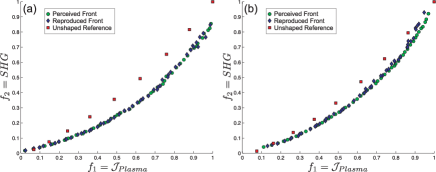
Figure 16: Experimental Pareto fronts for the Molecular Plasma Generation problem (maximizing free electron number $\mathcal{J}_{Plasma}$ versus minimizing $SHG$), for the MO-CMA with occasional re-evaluation [LEFT, (a)] and for the SMS-EMOA [RIGHT, (b)]. Each figure depicts the perceived front of a single experiment, the reference front of the intensity based non-shaped pulse, as well as the reproduction of the Pareto optimal set upon the termination of the run.

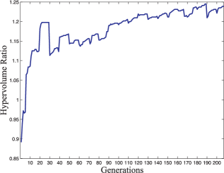
Figure 17: The evolving hypervolume pay-off of the parental population of the MO-CMA with re-evaluation every 10 generations, with respect to the unshaped reference front, corresponding to the run depicted in Fig. 16[(a)]. The periodic re-evaluation corrects fitness disturbances within the parental population, and causes the occasional hypervolume declines. It does not, however, hamper the general trend of hypervolume increase in the course of the entire run. For the hypervolume calculations, a reference point at $[0,1]$ was considered.

6 Summary

This paper introduced the topic of Multi-Observable Quantum Control and promoted its platform as a testbed for evolutionary experimental multi-objective optimization. It discussed various practical issues concerning this experimental domain, such as the sources of noise and uncertainty, and predominantly considered the MO-CMA as the optimization method. Several frameworks were targeted for testing – two noisy model landscapes, as well as multiple QC systems: one simulated and two experimental. Towards this end, we introduced here a family of test-functions, originating from the optical domain of Diffraction Grating problems, which can provide model landscapes for Pareto optimization. Their attractiveness lies particularly within the simple, yet full mathematical formulation as well as within the practical linkage to real-world experiments. Overall, this effort constituted a broad study of the MO-CMA, subject to fitness disturbance of noisy decision parameters on simulated systems, and its deployment in QC laboratory experiments.

While the MO-CMA excels in Pareto optimization of noise-free model landscapes, it has been observed in the current study that there exists a considerable discrepancy between the perceived Pareto front, given as the output by the algorithm, compared to the a posteriori evaluation of its pre-images, on both model landscapes. We proposed an explanation for this significant deviation, stating that the MO-CMA optimally exploits the disturbance distribution and converges to the minimal number of search points required to fully span the perceived front. As we demonstrated on the Bi-Sphere case, occasional parental fitness re-evaluation improved the MO-CMA performance and thus constituted a solution to the problem.

We set up a comparison between the MO-CMA and two conventional EMOA, namely NSGA-II and SMS-EMOA, on the Diffraction Grating test problem. While the MO-CMA was the clear winner in low search space dimensions, it suffered from slow progress rates in higher-dimensions ($n=80$), likely due to its self-adaptation mechanism, and required a significant increase in function evaluations in order to converge to the true Pareto front. In those cases, the SMS-EMOA performed better, and provided a fair approximate front within the original budget of function evaluations.

The application of the MO-CMA to the simulated noisy QC alignment system was successful in terms of revealing the physics conflict between the investigated objectives, and providing a reliable Pareto front considering the noise-free calculations. The quality of the Pareto optimal set was questionable, since the perceived front could not be recovered to a satisfactory degree. Concerning the reference algorithms, both SMS-EMOA and NSGA-II performed poorly in comparison to the MO-CMA, and failed to cover an important area of the Pareto front. The results here constitute an example of a scenario where there is clearly no best algorithm for a set of problems, especially when practical experimental requirements, e.g. a fixed budget of function evaluations, are imposed on the search. This observation can be considered as a practical interpretation to the so-called No Free Lunch (NFL) theorem (see, e.g., [61]).

The laboratory experiments – the practical climax of this work – allowed us to examine the proposed algorithmic framework in real-world experimental scenarios. We assessed the conflict between competing objectives for two experimental quantum systems, and provided interesting Pareto fronts which proved to be reliable with high confidence. The first experimental case of molecular ion generation considered only the default MO-CMA routine, due to instability and laboratory overhead. The Pareto front in this case could not be recovered upon evaluation of the Pareto optimal set, consistent with the previous observations of this work on model landscapes. The second experimental case on the molecular plasma generation system was extensively explored by means of various EMOA, and the results led to important practical conclusions. The MO-CMA with occasional parental re-evaluation performed best, obtained an excellent pay-off with respect to the standard unshaped reference, and the reproduction of its attained Pareto front was successful. Examination of its evolving hypervolume revealed the self-correcting property of the re-evaluation scheme, which overall proved to be essential in this experimental scenario. We therefore conclude that the MO-CMA with occasional re-evaluation, which introduces a basic yet effective extension to an existing EMOA, constitutes a powerful and reliable routine for experimental high-dimensional continuous Pareto optimization.

We would like to propose lines of future work. Given the conclusions drawn here, the formulation of algorithmic solutions for the MO-CMA is needed. In addition, sensitivity of auxiliary strategy parameters, including a parameter that was introduced here (the parental re-evaluation interval) should be investigated. In a different direction, future research may also incorporate into multi-objective experimental optimization advanced features that have the potential to capture various decision making preferences, such as Pareto-compliant indicators [62], or the enhancement of decision space diversity [63, 64].

Appendix 0.A The Diffraction Grating Problem: Analytical Expression of the 2-Dimensional Pareto Front

We consider here a specific instantiation of the Diffraction Grating problem, as formulated in Eq. 17 with $b=1,~{}h=4$. Let $n\in\mathbb{N}$ and $n\geq 2$, we then define:

$$\begin{array}[]{l}\vskip 6.0pt plus 2.0pt minus 2.0pt\displaystyle\jmath_{1}=J_{DG}\left(0,\vec{\varphi}\right)=n+2\cdot\sum_{n>\ell>k\geq 0}\cos\left[\varphi_{l}-\varphi_{k}\right]\\ \displaystyle\jmath_{2}=J_{DG}\left(\frac{\pi}{4},\vec{\varphi}\right)=n+2\cdot\sum_{n>\ell>k\geq 0}\cos\left[\pi\left(\ell-k\right)+\varphi_{l}-\varphi_{k}\right]\end{array}$$ (25)

Let:

$$D=\{(x,y)\in\mathbb{R}^{2}~{}\backslash~{}\exists\vec{\varphi}\in[0~{}2\pi]^{n}:x=\jmath_{1}(\vec{\varphi})\wedge y=\jmath_{2}(\vec{\varphi})\}$$

Theorem 1

The Pareto front $PF(\vec{\jmath})$ of $\vec{\jmath}(\vec{\varphi})=(\jmath_{1}(\vec{\varphi}),\jmath_{2}(\vec{\varphi}))^{T}$ for $\vec{\varphi}\in[0~{}2\pi]^{n}$ is

$$PF(\vec{\jmath})=\{(\jmath_{1},\jmath_{2})^{T}\in[\delta~{}n^{2}]^{2}~{}\backslash~{}\jmath_{1}+\jmath_{2}=n^{2}+\delta\}$$ (26)

with

$$\delta=\left\{\begin{array}[]{ll}0&\textrm{if}\>n=2\imath,~{}\imath\in\mathbb{N}\\ 1&\textrm{otherwise}\end{array}\right.\textrm{}$$

Proof

Let us consider $n$ even (i.e., $\delta=0$), the proof for $n$ odd is similar. The proof is carried out in two steps:

• We prove that $D\subset F=\{(x,y)\in[0~{}n^{2}]^{2}~{}\backslash~{}x+y\leq n^{2}\}$

• We prove that $\forall(x,y)\in F$ such that

  $$x+y=n^{2}\exists\vec{\varphi}\in[0~{}2\pi]^{n}$$

  with $x=\jmath_{1}(\vec{\varphi})$ and $y=\jmath_{2}(\vec{\varphi})$.

First, notice that:

$$\jmath_{1}(\vec{\varphi})=\left|\sum_{k=0}^{n-1}{e^{i\varphi_{k}}}\right|^{2},~{}~{}~{}\jmath_{2}(\vec{\varphi})=\left|\sum_{k=0}^{n-1}{(-1)^{k}e^{i\varphi_{k}}}\right|^{2}$$

Hence, $\forall\vec{\varphi}\in[0~{}2\pi]^{n}$ $\jmath_{1}\geq 0$ and $\jmath_{2}\geq 0$.
We start by rewriting the functions $\jmath_{1}$ and $\jmath_{2}$ in order to eliminate the $\pi$ factor in the cosine arguments of $\jmath_{2}$:

$$\jmath_{1}(\varphi_{0},...,\varphi_{n-1}) = n+2\cdot\sum_{k=0}^{n-2}{\sum_{l=k+1}^{n-1}{\cos\left[\varphi_{l}-\varphi_{k}\right]}}$$

$$\jmath_{2}(\varphi_{0},...,\varphi_{n-1}) = n+2\cdot\sum_{k=0}^{n-2}{\sum_{l=k+1}^{n-1}{\cos\left[\pi(l-k)+\varphi_{l}-\varphi_{k}\right]}}$$

$$\jmath_{1}(\varphi_{0},...,\varphi_{n-1}) = n+2\cdot\sum_{k=0}^{n-2}{\sum_{l=1}^{n-1-k}{\cos\left[\varphi_{k+l}-\varphi_{k}\right]}}$$

$$\jmath_{2}(\varphi_{0},...,\varphi_{n-1}) = n+2\cdot\sum_{k=0}^{n-2}{\sum_{l=1}^{n-1-k}{\cos\left[\pi l+\varphi_{k+l}-\varphi_{k}\right]}}$$

Since $n$ is even and greater than $2$, $\exists m\in\mathbb{N}$ $n=2(m+1)$.

$$\begin{array}[]{l}\displaystyle\frac{1}{2}\jmath_{1}(\varphi_{0},\ldots,\varphi_{n-1})=(m+1)+\sum_{p=0}^{m}\sum_{l=1}^{2m+1-2p}{\cos\left[\varphi_{2p+l}-\varphi_{2p}\right]}+\sum_{p=0}^{m-1}\sum_{l=1}^{2m-2p}{\cos\left[\varphi_{2p+1+l}-\varphi_{2p+1}\right]}\\ \displaystyle\frac{1}{2}\jmath_{2}(\varphi_{0},\ldots,\varphi_{n-1})=(m+1)+\sum_{p=0}^{m}\sum_{l=1}^{2m+1-2p}{\cos\left[l\pi+\varphi_{2p+l}-\varphi_{2p}\right]}+\sum_{p=0}^{m-1}\sum_{l=1}^{2m-2p}{\cos\left[l\pi+\varphi_{2p+1+l}-\varphi_{2p+1}\right]}\end{array}$$ (27)

$$\begin{array}[]{l}\displaystyle\frac{1}{2}\jmath_{1}(\varphi_{0},...,\varphi_{n-1})=(m+1)\sum_{p=0}^{m}\sum_{q=0}^{m-p}{\cos\left[\varphi_{2p+2q+1}-\varphi_{2p}\right]}+\sum_{p=0}^{m-1}\sum_{q=1}^{m-p}{\cos\left[\varphi_{2p+2q}-\varphi_{2p}\right]}\\ \displaystyle~{}~{}~{}~{}~{}+\sum_{p=0}^{m-1}\sum_{q=0}^{m-p-1}{\cos\left[\varphi_{2p+2+2q}-\varphi_{2p+1}\right]}+\sum_{p=0}^{m-1}\sum_{q=1}^{m-p}{\cos\left[\varphi_{2p+1+2q}-\varphi_{2p+1}\right]}\\ \displaystyle\frac{1}{2}\jmath_{2}(\varphi_{0},...,\varphi_{n-1})=(m+1)-\sum_{p=0}^{m}\sum_{q=0}^{m-p}{\cos\left[\varphi_{2p+2q+1}-\varphi_{2p}\right]}+\sum_{p=0}^{m-1}\sum_{q=1}^{m-p}{\cos\left[\varphi_{2p+2q}-\varphi_{2p}\right]}\\ \displaystyle~{}~{}~{}~{}~{}-\sum_{p=0}^{m}\sum_{q=0}^{m-p-1}{\cos\left[\varphi_{2p+2+2q}-\varphi_{2p+1}\right]}+\sum_{p=0}^{m-1}\sum_{q=1}^{m-p}{\cos\left[\varphi_{2p+1+2q}-\varphi_{2p+1}\right]}\end{array}$$ (28)

Upon considering all the cosines having values of $\pm 1$, we may write:

$$D\subset\left[0~{}n^{2}\right]^{2}$$

Moreover, we have:

$$\frac{1}{2}(\jmath_{1}+\jmath_{2})=2(m+1)+2\sum_{p=0}^{m-1}\sum_{q=1}^{m-p}{\cos\left[\varphi_{2p+2q}-\varphi_{2p}\right]}+2\sum_{p=0}^{m-1}\sum_{q=1}^{m-p}{\cos\left[\varphi_{2p+1+2q}-\varphi_{2p+1}\right]}$$ (29)

which leads to:

$$\jmath_{1}+\jmath_{2}\leq n^{2}$$ (30)

Hence,

$$D\subset F=\left\{\left(x,y\right)\in\left[0~{}n^{2}\right]^{2}~{}\backslash~{}x+y\leq n^{2}\right\}$$ (31)

In what follows, we shall show that this upper bound is indeed reached:
Given $L=\frac{1}{2}(\jmath_{1}+\jmath_{2})$, it reaches its global maximum if and only if, $\forall p\in[0~{}m]$ and $l$ such that $2p+2l\leq n$ and $2p+1+2l\leq n-1$ $\exists k_{ij},k^{\prime}_{ij}\in\mathbb{Z}$ such that:

$$\varphi_{2p+2l} = \varphi_{2p}+2k_{lp}\pi$$ (32)

$$\varphi_{2p+1+2l} = \varphi_{2p+1}+2k^{\prime}_{lp}\pi$$ (33)

Let us consider $\vec{\varphi}$ satisfying Eq. 32 and Eq. 33:

$$\jmath_{1}(\varphi_{0},...,\varphi_{n-1}) = \frac{1}{2}n^{2}(1+\cos(\varphi_{1}-\varphi_{0}))$$

$$\jmath_{2}(\varphi_{0},...,\varphi_{n-1}) = \frac{1}{2}n^{2}(1-\cos(\varphi_{1}-\varphi_{0})),$$

where $\varphi_{1}-\varphi_{0}$ takes any value in $[0~{}2\pi]$. Since $\theta\in[0~{}2\pi]\rightarrow\cos(\theta)\in[-1~{}1]$ is a surjective function, we can conclude that for all $(x,y)\in[0~{}n^{2}]^{2}$ such that $x+y=n^{2}~{}\exists\vec{\varphi}\in[0~{}2\pi]^{n}$ such that $x=\jmath_{1}(\vec{\varphi})$ and $y=\jmath_{2}(\vec{\varphi})$. This concludes the proof.

Appendix 0.B Diffraction Grating: Noise Propagation

We provide here explicit calculations of the mean and variance for the perceived objective function of the Diffraction Grating model landscape, described in Section 4.

0.B.1 Diffraction Grating: Mean

Consider the intensity function, $I_{DG}$, presented in Eq. 15, which may be written as

$$\begin{array}[]{l}\vskip 6.0pt plus 2.0pt minus 2.0pt\displaystyle I_{DG}\left(\zeta,\vec{\varphi}\right)=\frac{1}{n^{2}}\textrm{sinc}^{2}\left(\frac{\zeta b}{2}\right)\cdot J_{DG}\left(\zeta,\vec{\varphi}\right)\\ \displaystyle J_{DG}\left(\zeta,\vec{\varphi}\right)=n+2\cdot\sum_{\ell>k}\cos\left[\zeta h\left(\ell-k\right)+\Delta\varphi_{\ell k}\right]\end{array}$$ (34)

where the compact double-sum notation is used for convenience. Given a disturbed phase vector, $\tilde{\vec{\varphi}}$, following Eq. 18,

$$\tilde{\vec{\varphi}}=\left(\varphi_{0}+\delta\varphi_{0},\varphi_{1}+\delta\varphi_{1},\ldots,\varphi_{n-1}+\delta\varphi_{n-1}\right)^{T}$$ (35)

it thus suffices to investigate the propagation of the noise through $J_{DG}$ only:

$$\tilde{J}_{DG}\left(\zeta,\tilde{\vec{\varphi}}\right)=n+2\cdot\sum_{\ell>k}\cos\left[\zeta h\left(\ell-k\right)+\Delta\tilde{\varphi}_{\ell k}\right]$$ (36)

Note that

$$\begin{array}[]{l}\vskip 6.0pt plus 2.0pt minus 2.0pt\displaystyle\delta\varphi_{\ell}\sim\mathcal{N}\left(0,\epsilon^{2}\right)\\ \displaystyle\delta\varphi_{\ell k}\equiv\delta\varphi_{\ell}-\delta\varphi_{k}\sim\mathcal{N}\left(0,2\epsilon^{2}\right)\end{array}$$ (37)

Given the probability density function of the normal distribution, denoted as $\Phi(z,\mu,\sigma^{2})$, the expectation values of the cosine and sine functions considering a distribution with zero mean read:

$$\begin{array}[]{l}\vskip 6.0pt plus 2.0pt minus 2.0pt\displaystyle\int_{-\infty}^{\infty}\Phi(z,0,\sigma^{2})\cos(z)dz=\exp\left(-\frac{\sigma^{2}}{2}\right)\\ \displaystyle\int_{-\infty}^{\infty}\Phi(z,0,\sigma^{2})\sin(z)dz=0\end{array}$$ (38)

Eq. 36 can now be rewritten as:

$$\begin{array}[]{l}\vskip 6.0pt plus 2.0pt minus 2.0pt\displaystyle\tilde{J}_{DG}=n+2\cdot\sum_{\ell>k}\cos\left[\zeta h\left(\ell-k\right)+\Delta\varphi_{\ell k}+\delta\varphi_{\ell k}\right]=\\ \displaystyle=n+2\cdot\sum_{\ell>k}\cos\left(a_{\ell k}\right)\cos\left(\delta\varphi_{\ell k}\right)-\sin\left(a_{\ell k}\right)\sin\left(\delta\varphi_{\ell k}\right)\end{array}$$ (39)

where $a_{\ell k}\equiv\zeta h\left(\ell-k\right)+\Delta\varphi_{\ell k}$. Upon calculating the expectation values, using Eq. 38, one may write:

$$\begin{array}[]{l}\displaystyle\left<\tilde{J}_{DG}\right>=n+2\cdot\sum_{\ell>k}\cos\left(a_{\ell k}\right)\left<\cos\left(\delta\varphi_{\ell k}\right)\right>-2\cdot\sum_{\ell>k}\sin\left(a_{\ell k}\right)\left<\sin\left(\delta\varphi_{\ell k}\right)\right>=\\ \displaystyle=n+2\cdot\sum_{\ell>k}\cos\left(a_{\ell k}\right)\cdot\exp\left(-\epsilon^{2}\right)=n+2\cdot\exp\left(-\epsilon^{2}\right)\cdot\sum_{\ell>k}\cos\left(a_{\ell k}\right),\end{array}$$ (40)

concluding with

$$\boxed{\displaystyle\left<\tilde{J}_{DG}\right>=n\cdot\left(1-\exp\left(-\epsilon^{2}\right)\right)+\exp\left(-\epsilon^{2}\right)\cdot J_{DG}}$$ (41)

The transition to $\left<\tilde{I}_{DG}\right>$ is trivial with Eq. 34, yielding the result of Eq. 19.

0.B.2 Diffraction Grating: Variance

$$\textrm{VAR}\left[\tilde{J}_{DG}\right]=\left<{\tilde{J}_{DG}}^{2}\right>-\left<\tilde{J}_{DG}\right>^{2}$$

From Eq. 41, $\left<\tilde{J}_{DG}\right>^{2}$ is trivial. We now have to compute $\left<{\tilde{J}_{DG}}^{2}\right>$. In order to do so, let us first compute the mean of this easier term:

$$\begin{array}[]{l}\left(\frac{\tilde{J}_{DG}-n}{2}\right)^{2}=\\ \sum_{l_{1}>k_{1}}\sum_{l_{2}>k_{2}}\left(\cos(a_{l_{1}k_{1}})\cos(\delta\varphi_{l_{1}k_{1}})-\sin(a_{l_{1}k_{1}})\sin(\delta\varphi_{l_{1}k_{1}})\right)\\ \left(\cos(a_{l_{2}k_{2}})\cos(\delta\varphi_{l_{2}k_{2}})-\sin(a_{l_{2}k_{2}})\sin\left(\delta\varphi_{l_{2}k_{2}}\right)\right)\end{array}$$

Let (for $j=1,2$)

$$c_{j}^{a}=\cos(a_{l_{j}k_{j}})~{},s_{j}^{a}=\sin(a_{l_{j}k_{j}})~{},c_{j}^{d}=\cos(\delta\varphi_{l_{j}k_{j}})~{},c_{j}^{d}=\cos(\delta\varphi_{l_{j}k_{j}})$$

$$\Gamma_{l_{1}l_{2}k_{1}k_{2}}=c_{1}^{a}c_{2}^{a}c_{1}^{d}c_{2}^{d}+s_{1}^{a}s_{2}^{a}s_{1}^{d}s_{2}^{d}-2c_{1}^{a}s_{2}^{a}c_{1}^{d}s_{2}^{d}$$

$$\left(\frac{\tilde{J}_{DG}-n}{2}\right)^{2}=\sum_{l_{1}>k_{1}}\sum_{l_{2}>k_{2}}\Gamma_{l_{1}l_{2}k_{1}k_{2}}$$ (42)

We divide the set $LK=\{(l_{1},k_{1},l_{2},k_{2})\in\left[0\ldots n-1\right]^{4}/l_{1}>k_{1}\wedge l_{2}>k_{2}\}$, to which belong $(l_{1},k_{1},l_{2},k_{2})$, into the six following subsets which form a partition:

$$LK=LK_{indpt}\cup LK_{lklk}\cup LK_{l.l.}\cup LK_{l..l}\cup LK_{.k.k}\cup LK_{.kk.}$$

Consequently, the sum in Eq. 42 may be divided into six sums, and we note:

$$\begin{array}[]{l}\left(\frac{\tilde{J}_{DG}-n}{2}\right)^{2}=\sum_{LK_{indpt}}\Gamma_{l_{1}l_{2}k_{1}k_{2}}+\sum_{LK_{lklk}}\Gamma_{l_{1}l_{2}k_{1}k_{2}}+\sum_{LK_{l.l.}}\Gamma_{l_{1}l_{2}k_{1}k_{2}}\\ +\sum_{LK_{l..l}}\Gamma_{l_{1}l_{2}k_{1}k_{2}}+\sum_{LK_{.k.k}}\Gamma_{l_{1}l_{2}k_{1}k_{2}}+\sum_{LK_{.kk.}}\Gamma_{l_{1}l_{2}k_{1}k_{2}}\end{array}$$

with

$$\begin{array}[]{l}LK_{indpt}=\{(l_{1},k_{1},l_{2},k_{2})\in\left[0\ldots n-1\right]^{4}/l_{1}>k_{1}\wedge l_{2}>k_{2}\wedge l_{1}\neq l_{2}\wedge l_{1}\neq k_{2}\wedge k_{1}\neq k_{2}\wedge k_{1}\neq l_{2}\}\\ LK_{lklk}=\{(l_{1},k_{1},l_{2},k_{2})\in\left[0\ldots n-1\right]^{4}/l_{1}>k_{1}\wedge l_{2}>k_{2}\wedge l_{1}=l_{2}\wedge k_{1}=k_{2}\}\\ LK_{l.l.}=\{(l_{1},k_{1},l_{2},k_{2})\in\left[0\ldots n-1\right]^{4}/l_{1}>k_{1}\wedge l_{2}>k_{2}\wedge l_{1}=l_{2}\wedge k_{1}\neq k_{2}\}\\ LK_{l..l}=\{(l_{1},k_{1},l_{2},k_{2})\in\left[0\ldots n-1\right]^{4}/l_{1}>k_{1}\wedge l_{2}>k_{2}\wedge l_{1}=k_{2}\}\\ LK_{.k.k}=\{(l_{1},k_{1},l_{2},k_{2})\in\left[0\ldots n-1\right]^{4}/l_{1}>k_{1}\wedge l_{2}>k_{2}\wedge k_{1}=k_{2}\wedge l_{1}\neq l_{2}\}\\ LK_{.kk.}=\{(l_{1},k_{1},l_{2},k_{2})\in\left[0\ldots n-1\right]^{4}/l_{1}>k_{1}\wedge l_{2}>k_{2}\wedge k_{1}=l_{2}\}\end{array}$$

Additionally, we note that

$$\begin{array}[]{l}\sharp(LK)=\left(\frac{n(n-1)}{2}\right)^{2}\\ \sharp(LK_{lklk})=\frac{n(n-1)}{2}\\ \sharp(LK_{l.l.})=\sharp(LK_{.k.k})=\\ \frac{1}{6}n(n-1)(2n-1)+\frac{1}{2}(3-2n)n(n-1)+n(n-1)(n-2)\\ \sharp(LK_{l..l})=\sharp(LK_{.kk.})=-\frac{1}{6}n(n-1)(2n-1)+\frac{1}{2}n(n-1)^{2}\\ \sharp(LK_{indpt})=\frac{n(n-1)}{2}\left(\frac{n(n-1)}{2}-2n+3\right)\end{array}$$

Explicit Summation

First, consider the following useful results:

$$\begin{array}[]{l}\left<\cos(\delta\varphi_{l})\right>=\exp\left(-\frac{\epsilon^{2}}{2}\right)\\ \left<\cos(\delta\varphi_{lk})\right>=\exp\left(-\epsilon^{2}\right)\\ \left<\sin(\delta\varphi_{lk})\right>=0\\ \left<\cos(2\delta\varphi_{lk})\right>=\exp\left(-4\epsilon^{2}\right)\\ \left<\cos(\delta\varphi_{lk})^{2}\right>=\frac{1}{2}\left(1+\exp\left(-4\epsilon^{2}\right)\right)\\ \left<\cos(\delta\varphi_{lk})\sin(\delta\varphi_{lr})\right>=0\\ \left<\sin(\delta\varphi_{lk})^{2}\right>=\frac{1}{2}\left(1-\exp\left(-4\epsilon^{2}\right)\right)\\ \left<\cos(\delta\varphi_{lk})\cos(\delta\varphi_{lr})\right>=\frac{1}{2}\left(1+\exp\left(-2\epsilon^{2}\right)\right)\exp\left(-\epsilon^{2}\right)\\ \left<\sin(\delta\varphi_{lk})\sin(\delta\varphi_{lr})\right>=\frac{1}{2}\left(1-\exp\left(-2\epsilon^{2}\right)\right)\exp\left(-\epsilon^{2}\right)\end{array}$$

We then have:

0.B.2.1 $LK_{indpdt}$

$$\begin{array}[]{l}\vskip 6.0pt plus 2.0pt minus 2.0pt\displaystyle\left<\sum_{LK_{indpdt}}\Gamma_{l_{1}l_{2}k_{1}k_{2}}\right>=\\ \vskip 6.0pt plus 2.0pt minus 2.0pt\displaystyle\sum_{LK_{indpdt}}{c_{1}^{a}c_{2}^{a}\left<c_{1}^{d}\right>\left<c_{2}^{d}\right>+s_{1}^{a}s_{2}^{a}\left<s_{1}^{d}\right>\left<s_{2}^{d}\right>-2c_{1}^{a}s_{2}^{a}\left<c_{1}^{d}\right>\left<s_{2}^{d}\right>}\\ \displaystyle=\exp\left(-2\epsilon^{2}\right)\sum_{LK_{indpdt}}{\cos(a_{l_{1}k_{1}})\cos(a_{l_{2}k_{2}})}\end{array}$$ (43)

0.B.2.2 $LK_{lklk}$

$$\begin{array}[]{l}\vskip 6.0pt plus 2.0pt minus 2.0pt\displaystyle\left<\sum_{LK_{lklk}}\Gamma_{l_{1}l_{2}k_{1}k_{2}}\right>=\\ \vskip 6.0pt plus 2.0pt minus 2.0pt\displaystyle\sum_{LK_{lklk}}{(c^{a})^{2}\left<(c^{d})^{2}\right>+(s^{a})^{2}\left<(s^{d})^{2}\right>-\frac{1}{2}s^{2a}\left<s^{2d}\right>}\\ \displaystyle=\frac{n(n-1)}{4}+\frac{\exp\left(-4\epsilon^{2}\right)}{2}\sum_{l>k}{\cos(2a_{lk})}\end{array}$$ (44)

0.B.2.3 $LK_{l.l.}$

$$\begin{array}[]{l}\vskip 6.0pt plus 2.0pt minus 2.0pt\displaystyle\left<\sum_{LK_{l.l.}}\Gamma_{l_{1}l_{2}k_{1}k_{2}}\right>=\\ \displaystyle\sum_{LK_{l.l.}}c_{1}^{a}c_{2}^{a}\left<\cos(\delta\varphi_{lk})\cos(\delta\varphi_{lr})\right>+s_{1}^{a}s_{2}^{a}\left<\sin(\delta\varphi_{lk})\sin(\delta\varphi_{lr})\right>\\ \vskip 6.0pt plus 2.0pt minus 2.0pt\displaystyle\quad\quad-2c_{1}^{a}s_{2}^{a}\left<\cos(\delta\varphi_{lk})\sin(\delta\varphi_{lr})\right>\\ \displaystyle=\frac{1}{2}\exp\left(-\epsilon^{2}\right)\sum_{LK_{l.l.}}{\cos(a_{lk}-a_{lr})+\exp\left(-2\epsilon^{2}\right)\cos(a_{lk}+a_{lr})}\end{array}$$ (45)

0.B.2.4 $LK_{l..l}$

$$\begin{array}[]{l}\vskip 6.0pt plus 2.0pt minus 2.0pt\displaystyle\left<\sum_{LK_{l..l}}\Gamma_{l_{1}l_{2}k_{1}k_{2}}\right>=\\ \displaystyle\sum_{LK_{l..l}}c_{1}^{a}c_{2}^{a}\left<\cos(\delta\varphi_{lk})\cos(\delta\varphi_{sl})\right>+s_{1}^{a}s_{2}^{a}\left<\sin(\delta\varphi_{lk})\sin(\delta\varphi_{sl})\right>\\ \vskip 6.0pt plus 2.0pt minus 2.0pt\displaystyle\quad\quad-2c_{1}^{a}s_{2}^{a}\left<\cos(\delta\varphi_{lk})\sin(\delta\varphi_{sl})\right>\\ \displaystyle=\frac{1}{2}\exp\left(-\epsilon^{2}\right)\sum_{LK_{l..l}}{\cos(a_{lk}+a_{lr})+\exp\left(-2\epsilon^{2}\right)\cos(a_{lk}-a_{lr})}\end{array}$$ (46)

0.B.2.5 $LK_{.k.k}$

$$\begin{array}[]{l}\vskip 6.0pt plus 2.0pt minus 2.0pt\displaystyle\left<\sum_{LK_{.k.k}}\Gamma_{l_{1}l_{2}k_{1}k_{2}}\right>=\\ \displaystyle\sum_{LK_{.k.k}}c_{1}^{a}c_{2}^{a}\left<\cos(\delta\varphi_{lk})\cos(\delta\varphi_{sk})\right>+s_{1}^{a}s_{2}^{a}\left<\sin(\delta\varphi_{lk})\sin(\delta\varphi_{sk})\right>\\ \vskip 6.0pt plus 2.0pt minus 2.0pt\displaystyle\quad\quad-2c_{1}^{a}s_{2}^{a}\left<\cos(\delta\varphi_{lk})\sin(\delta\varphi_{sk})\right>\\ \displaystyle=\frac{1}{2}\exp\left(-\epsilon^{2}\right)\sum_{LK_{.k.k}}{\cos(a_{lk}-a_{sk})+\exp\left(-2\epsilon^{2}\right)\cos(a_{lk}+a_{sk})}\end{array}$$ (47)

0.B.2.6 $LK_{.kk.}$

$$\begin{array}[]{l}\vskip 6.0pt plus 2.0pt minus 2.0pt\displaystyle\left<\sum_{LK_{.kk.}}\Gamma_{l_{1}l_{2}k_{1}k_{2}}\right>=\\ \displaystyle\sum_{LK_{.kk.}}c_{1}^{a}c_{2}^{a}\left<\cos(\delta\varphi_{lk})\cos(\delta\varphi_{ks})\right>+s_{1}^{a}s_{2}^{a}\left<\sin(\delta\varphi_{lk})\sin(\delta\varphi_{ks})\right>\\ \vskip 6.0pt plus 2.0pt minus 2.0pt\displaystyle\quad\quad-2c_{1}^{a}s_{2}^{a}\left<\cos(\delta\varphi_{lk})\sin(\delta\varphi_{ks})\right>\\ \displaystyle=\frac{1}{2}\exp\left(-\epsilon^{2}\right)\sum_{LK_{.kk.}}{\cos(a_{lk}+a_{ks})+\exp\left(-2\epsilon^{2}\right)\cos(a_{lk}-a_{ks})}\end{array}$$ (48)

Conclusion

From Eqs. 43, 44, 45, 46, 47, 48 we may write:

$$\begin{array}[]{l}\vskip 6.0pt plus 2.0pt minus 2.0pt\displaystyle\left<\left(\frac{\tilde{J}_{DG}-n}{2}\right)^{2}\right>=\frac{n(n-1)}{4}+\frac{\exp\left(-4\epsilon^{2}\right)}{2}\sum_{l>k}{\cos(2a_{lk})}+\exp\left(-2\epsilon^{2}\right)\sum_{LK_{indpdt}}{\cos(a_{lk})\cos(a_{rs})}\\ \displaystyle+\frac{1}{2}\exp\left(-\epsilon^{2}\right)\left[\sum_{LK_{l.l.}\cup LK_{.k.k}}{\cos(a_{lk}-a_{rs})+\exp\left(-2\epsilon^{2}\right)\cos(a_{lk}+a_{rs})}\right.\\ \displaystyle\left.+\sum_{LK_{l..l}\cup LK_{.kk.}}{\cos(a_{lk}+a_{rs})+\exp\left(-2\epsilon^{2}\right)\cos(a_{lk}-a_{rs})}\right]\end{array}$$ (49)

concluding with:

$$\boxed{\begin{array}[]{l}\vskip 6.0pt plus 2.0pt minus 2.0pt\displaystyle\textrm{VAR}\left[\tilde{J}_{DG}\right]=n(n-1)\left(1-\exp\left(-2\epsilon^{2}\right)\right)-2\exp\left(-2\epsilon^{2}\right)\left(1-\exp\left(-2\epsilon^{2}\right)\right)\sum_{l>k}{\cos(2a_{lk})}\\ \displaystyle+2\exp\left(-\epsilon^{2}\right)\left(1-\exp\left(-\epsilon^{2}\right)\right)\left[\sum_{LK_{l.l.}\cup LK_{.k.k}}{\cos(a_{lk}-a_{rs})}+\sum_{LK_{l..l}\cup LK_{.kk.}}{\cos(a_{lk}+a_{rs})}\right]\\ \displaystyle-2\exp\left(-2\epsilon^{2}\right)\left(1-\exp\left(-\epsilon^{2}\right)\right)\left[\sum_{LK_{l.l.}\cup LK_{.k.k}}{\cos(a_{lk}+a_{rs})}+\sum_{LK_{l..l}\cup LK_{.kk.}}{\cos(a_{lk}-a_{rs})}\right]\end{array}}$$ (50)

An upper bound on the variance is given by:

$$\textrm{VAR}\left[\tilde{J}_{DG}\right]\leq n(n-1)\left[\left(1-\exp\left(-4\epsilon^{2}\right)\right)+2\exp\left(-\epsilon^{2}\right)\left(1-\exp\left(-2\epsilon^{2}\right)\right)(n-2)\right]$$ (51)

For a small $\epsilon$, the bound may be tightened:

$$\textrm{VAR}\left[\tilde{J}_{DG}\right]\leq 4n(n-1)^{2}\epsilon^{2}$$ (52)

Note that in order to obtain Eq. 52 , all the cosine terms had to be majored by $1$. Given a point on the screen with destructive interference (the sum and products of the cosines vanish), the upper bound in Eq. 52 is strongly superior with respect to the actual variance. On the other hand, given a point with constructive interference, the upper bound is a fair estimation of the real variance. Notice also that the upper bound of the variance is proportional to the cube of the dimension and the variance of the stochastic noise.

Finally, the transition to $\tilde{I}_{DG}$ is obtained:

$$\textrm{VAR}\left[\tilde{I}_{DG}\right]=\frac{1}{n^{4}}\textrm{sinc}^{4}\left(\frac{\zeta b}{2}\right)\cdot\textrm{VAR}\left[\tilde{J}_{DG}\right]$$ (53)

References

- [1] Warren, W.S., Rabitz, H., Dahleh, M.: Coherent Control of Quantum Dynamics: The Dream Is Alive. Science 259 (1993) 1581–1589
- [2] Nuernberger, P., Vogt, G., Brixner, T., Gerber, G.: Femtosecond Quantum Control of Molecular Dynamics in the Condensed Phase. Phys Chem Chem Phys. 9(20) (2007) 2470–2497
- [3] Weiner, A.M.: Femtosecond pulse shaping using spatial light modulators. Review of Scientific Instruments 71(5) (2000) 1929–1960
- [4] Peirce, A.P., Dahleh, M.A., Rabitz, H.: Optimal Control of Quantum-Mechanical Systems: Existence, Numerical Approximation, and Applications. Phys. Rev. A 37(12) (1988)
- [5] Judson, R.S., Rabitz, H.: Teaching Lasers to Control Molecules. Phys. Rev. Lett. 68(10) (1992) 1500–1503
- [6] Bäck, T.: Evolutionary Algorithms in Theory and Practice. Oxford University Press, New York, NY, USA (1996)
- [7] Klockgether, J., Schwefel, H.P.: Two-phase nozzle and hollow core jet experiments. In: Proceedings of the 11th Symposium on Engineering Aspects of Magneto-Hydrodynamics, Pasadena, California, USA, Caltech (1970)
- [8] Deb, K.: Multi-Objective Optimization Using Evolutionary Algorithms. Wiley, New York (2001)
- [9] Coello, C.A.C., Lamont, G.B., van Veldhuizen, D.A.: Evolutionary Algorithms for Solving Multiobjective Problems. Springer, Berlin (2007)
- [10] Knowles, J., Corne, D., Deb, K.: Multiobjective Problem Solving from Nature: From Concepts to Applications. Natural Computing Series. Springer, Berlin (2008)
- [11] Weber, S., Sauer, F., Plewicki, M., Merli, A., Wöste, L., Lindinger, A.: Multi-objective optimization on alkali dimers. Journal of Modern Optics 54(16-17) (2007) 2659–2666
- [12] Bonacina, L., Extermann, J., Rondi, A., Boutou, V., Wolf, J.P.: Multiobjective genetic approach for optimal control of photoinduced processes. Phys. Rev. A 76(2) (2007) 023408
- [13] Roth, M., Guyon, L., Roslund, J., Boutou, V., Courvoisier, F., Wolf, J.P., Rabitz, H.: Quantum control of tightly competitive product channels. Physical Review Letters 102(25) (2009) 253001
- [14] Bartelt, A., Roth, M., Mehendale, M., Rabitz, H.: Assuring robustness to noise in optimal quantum control experiments. Phys. Rev. A 71(6) (2005) 063806
- [15] Chakrabarti, R., Wu, R., Rabitz, H.: Quantum Pareto optimal control. Phys. Rev. A 78(3) (2008) 033414
- [16] Hansen, N., Kern, S.: Evaluating the CMA Evolution Strategy on Multimodal Test Functions. In: Parallel Problem Solving from Nature - PPSN V. Volume 1498 of Lecture Notes in Computer Science., Amsterdam, Springer (1998) 282–291
- [17] Shir, O.M., Roslund, J., Bäck, T., Rabitz, H.: Performance Analysis of Derandomized Evolution Strategies in Quantum Control Experiments. In: Proceedings of the Genetic and Evolutionary Computation Conference, GECCO-2008, New York, NY, USA, ACM Press (2008) 519–526
- [18] Wilson, J.W., Schlup, P., Lunacek, M., Whitley, D., Bartels, R.A.: Calibration of liquid crystal ultrafast pulse shaper with common-path spectral interferometry and application to coherent control with a covariance matrix adaptation evolutionary strategy. Review of Scientific Instruments 79(3) (2008) 033103+
- [19] Igel, C., Hansen, N., Roth, S.: Covariance Matrix Adaptation for Multi-objective Optimization. Evolutionary Computation 15(1) (2007) 1–28
- [20] Arnold, D.V.: Noisy Optimization with Evolution Strategies. Genetic Algorithms and Evolutionary Computation. Springer, Berlin (2002)
- [21] Ong, Y.S., Zhou, Z., Lim, D.: Curse and blessing of uncertainty in evolutionary algorithm using approximation. In: Proceedings of the 2006 IEEE World Congress on Computational Intelligence, IEEE Computational Intelligence Society (2006) 2928–2935
- [22] Beyer, H.G., Sendhoff, B.: Robust Optimization - A Comprehensive Survey. Computer Methods in Applied Mechanics and Engineering 196(33-34) (2007) 3190–3218
- [23] Branke, J.: Evolutionary Optimization in Dynamic Environments. Kluwer Academic Publishers, Norwell, MA, USA (2001)
- [24] Beyer, H.G., Sendhoff, B.: Evolution strategies for robust optimization. In: Proceedings of the 2006 IEEE World Congress on Computational Intelligence, IEEE Computational Intelligence Society (2006) 1346–1353
- [25] Beyer, H.G., Olhofer, M., Sendhoff, B.: On the Impact of Systematic Noise on the Evolutionary Optimization Performance—A Sphere Model Analysis. Genetic Programming and Evolvable Machines 5(4) (2004) 327–360
- [26] Deb, K., Gupta, H.: Introducing Robustness in Multi-Objective Optimization. Evolutionary Computation 14(4) (2006) 463–494
- [27] Teich, J.: Pareto Front Exploration with Uncertain Objectives. In: EMO ’01: Proceedings of the First International Conference on Evolutionary Multi-Criterion Optimization, London, UK, Springer-Verlag (2001) 314–328
- [28] Hughes, E.: Evolutionary Multi-objective Ranking with Uncertainty and Noise. In: EMO ’01: Proceedings of the First International Conference on Evolutionary Multi-Criterion Optimization, London, UK, Springer-Verlag (2001) 329–343
- [29] Büche, D., Stoll, P., Dornberger, R., Koumoutsakos, P.: Multiobjective Evolutionary Algorithm for the Optimization of Noisy Combustion Processes. Systems, Man, and Cybernetics, Part C: Applications and Reviews, IEEE Transactions on 32(4) (2002) 460–473
- [30] Goh, C.K., Tan, K.C.: An Investigation on Noisy Environments in Evolutionary Multiobjective Optimization. IEEE Transactions on Evolutionary Computation 11(3) (2007) 354–381
- [31] Bader, J., Zitzler, E.: Robustness in Hypervolume-based Multiobjective Search. TIK Report 317, Computer Engineering and Networks Laboratory (TIK), ETH Zurich (2010)
- [32] Mulvey, J.M., Vanderbei, R.J., Zenios, S.A.: Robust Optimization of Large-Scale Systems. Operations Research 43(2) (1995) 264–281
- [33] Egorov, I.N., Kretinin, G.V., Leshchenko, I.A.: How to Execute Robust Design Optimization. In: 9th AIAA/ISSMO Symposium and Exhibit on Multidisciplinary Analysis and Optimization. (2002)
- [34] Jin, Y., Sendhoff, B.: Trade-Off between Performance and Robustness: An Evolutionary Multiobjective Approach. In: Proc. Evolutionary Multi-Criterion Optimization: Second Int’l Conference (EMO 2003). Volume 2632 of Lecture Notes in Computer Science., Berlin, Springer (2003) 237–251
- [35] Gunawan, S., Azarm, S.: Multi-Objective Robust Optimization Using a Sensitivity Region Concept. Structural and Multidisciplinary Optimization 29(1) (2005) 50–60
- [36] Hagan, S.O., Dunn, W.B., Knowles, J.D., Broadhurst, D., Williams, R., Ashworth, J.J., Cameron, M., Kell, D.B.: Closed-Loop, Multiobjective Optimization of Two-Dimensional Gas Chromatography/Mass Spectrometry for Serum Metabolomics. Anal. Chem. 79(2) (2007) 464–476
- [37] Knowles, J.: Closed-loop evolutionary multiobjective optimization. IEEE Computational Intelligence Magazine (2009) 77–91
- [38] Knowles, J.: ParEGO: A Hybrid Algorithm with On-Line Landscape Approximation for Expensive Multiobjective Optimization Problems. IEEE Transactions on Evolutionary Computation 10(1) (2006) 50–66
- [39] van Veldhuizen, D.A., Lamont, G.B.: Multiobjective evolutionary algorithms: Analyzing the state-of-the-art. Evolutionary Computation 8(2) (2000) 125–147
- [40] Zitzler, E., Laumanns, M., Bleuler, S.: A Tutorial on Evolutionary Multiobjective Optimization. In: Metaheuristics for Multiobjective Optimisation. Volume 535 of Lecture Notes in Economics and Mathematical Systems., Springer (2004) 3–37
- [41] Igel, C., Suttorp, T., Hansen, N.: A Computational Efficient Covariance Matrix Update and a (1+1)-CMA for Evolution Strategies. In: Proceedings of the Genetic and Evolutionary Computation Conference, GECCO 2006, New York, NY, USA, ACM Press (2006) 453–460
- [42] Arnold, D.V., Beyer, H.G.: Local Performance of the -ES in a Noisy Environment. In Martin, W., Spears, W., eds.: Foundations of Genetic Algorithms, 6, San Francisco, CA, Morgan Kaufmann (2001) 127–141
- [43] Beyer, H.G.: Toward a Theory of Evolution Strategies: Some Asymptotical Results from the -Theory. Evolutionary Computation 1(2) (1993) 165–188
- [44] Arnold, D.V., Beyer, H.G.: Local performance of the (1 + 1)-ES in a noisy environment. IEEE Transactions on Evolutionary Computation 6(1) (2002) 30–41
- [45] Laumanns, M., Rudolph, G., Schwefel, H.P.: Mutation control and convergence in evolutionary multi-objective optimization. In: Proceedings of the 7th International Mendel Conference on Soft Computing (MENDEL 2001), Brno, Czech Republic (2001) 24–29
- [46] Emmerich, M., Deutz, A.: Test Problems Based on Lamé Superspheres. In: EMO-2007. Volume 4403 of Lecture Notes in Computer Science., Springer (2007) 922–936
- [47] Shir, O.M., Bäck, T., Rabitz, H., Vrakking, M.J.: On the Evolution of Laser Pulses under a Dynamic Quantum Control Environment. In: Proceedings of the 2008 IEEE World Congress on Computational Intelligence (WCCI-CEC), IEEE Computational Intelligence Society (2008) 2127–2134
- [48] Shir, O.M., Beltrani, V., Bäck, T., Rabitz, H., Vrakking, M.J.: On the Diversity of Multiple Optimal Controls for Quantum Systems. Journal of Physics B: Atomic, Molecular and Optical Physics 41(7) (2008) 074021
- [49] Shir, O.M., Emmerich, M., Bäck, T., Vrakking, M.J.: The Application of Evolutionary Multi-Criteria Optimization to Dynamic Molecular Alignment. In: Proceedings of the 2007 IEEE Congress on Evolutionary Computation (CEC), IEEE Computational Intelligence Society (2007) 4108–4115
- [50] Klinkenberg, J.W., Emmerich, M., Deutz, A., Shir, O.M., Bäck, T.: Accelerating SMS-EMOA for Problems with Time-Expensive Evaluations using Kriging, Self-Adaptation, and MPI. In: Multiple Criteria Decision Making for Sustainable Energy and Transportation Systems: Proceedings of MCDM 2008, The 19th International Conference on Multiple Criteria Decision Making. Volume 634 of Lecture Notes in Economics and Mathematical Systems., Heidelberg, Germany, Springer Physica-Verlag (2010) 301–312
- [51] Rosca-Pruna, F., Vrakking, M.J.: Revival Structures in Picosecond Laser-Induced Alignment of I2 Molecules. Journal of Chemical Physics 116(15) (2002) 6579–6588
- [52] Preuss, M.: Reporting on Experiments in Evolutionary Computation. Technical Report CI-221/07, University of Dortmund, SFB 531 (2007)
- [53] Igel, C., Glasmachers, T., Heidrich-Meisner, V.: Shark. Journal of Machine Learning Research 9 (2008) 993–996
- [54] Zitzler, E., Thiele, L.: Multiobjective Optimization Using Evolutionary Algorithms - A Comparative Case Study. In: Conference on Parallel Problem Solving from Nature (PPSN V). Volume 1498 of Lecture Notes in Computer Science., Amsterdam, Springer (1998) 292–301
- [55] Zitzler, E., Thiele, L., Laumanns, M., Fonseca, C.M., Grunert da Fonseca, V.: Performance Assessment of Multiobjective Optimizers: An Analysis and Review. IEEE Transactions on Evolutionary Computation 7(2) (2003) 117–132
- [56] Zitzler, E.: Evolutionary Algorithms for Multiobjective Optimization: Methods and Applications. PhD thesis, ETH Zurich, Switzerland (1999)
- [57] Laumanns, M., Rudolph, G., Schwefel, H.P.: Approximating the Pareto Set: Concepts, Diversity Issues, and Performance Assessment. Technical Report CI-72/99, University of Dortmund (1999)
- [58] Emmerich, M., Beume, N., Naujoks, B.: An EMO Algorithm using the Hypervolume Measure as Selection Criterion. In: Proc. Evolutionary Multi-Criterion Optimization: Third Int’l Conference (EMO 2005). Volume 3410 of Lecture Notes in Computer Science., Berlin, Springer (2005) 62–76
- [59] Ostermeier, A., Gawelczyk, A., Hansen, N.: Step-Size Adaptation Based on Non-Local Use of Selection Information. In: Parallel Problem Solving from Nature - PPSN III. Volume 866 of Lecture Notes in Computer Science., Springer (1994) 189–198
- [60] Ros, R., Hansen, N.: A Simple Modification in CMA-ES Achieving Linear Time and Space Complexity. In: Parallel Problem Solving from Nature - PPSN X. Volume 5199 of Lecture Notes in Computer Science., Springer (2008) 296–305
- [61] Wolpert, D.H., Macready, W.G.: No Free Lunch Theorems for Optimization. IEEE Transactions on Evolutionary Computation 1 (1997) 67–82
- [62] Zitzler, E., Brockhoff, D., Thiele, L.: The Hypervolume Indicator Revisited: On the Design of Pareto-compliant Indicators Via Weighted Integration. In Obayashi, S., et al., eds.: Conference on Evolutionary Multi-Criterion Optimization (EMO 2007). Volume 4403 of LNCS., Berlin, Springer (2007) 862–876
- [63] Shir, O.M., Preuss, M., Naujoks, B., Emmerich, M.: Enhancing Decision Space Diversity in Evolutionary Multiobjective Algorithms. In: Proceedings of Evolutionary Multi-Criterion Optimization: Fifth International Conference (EMO 2009). Volume 5467 of Lecture Notes in Computer Science., Springer (2009) 95–109
- [64] Ulrich, T., Bader, J., Zitzler, E.: Integrating decision space diversity into hypervolume-based multiobjective search. In: GECCO ’10: Proceedings of the 12th annual conference on Genetic and evolutionary computation, New York, NY, USA, ACM (2010) 455–462