Unbiased shifts of Brownian motion

Abstract

Let $B=(B_{t})_{t\in{\mathbb{R}}}$ be a two-sided standard Brownian motion. An unbiased shift of $B$ is a random time $T$, which is a measurable function of $B$, such that $(B_{T+t}-B_{T})_{t\in{\mathbb{R}}}$ is a Brownian motion independent of $B_{T}$. We characterise unbiased shifts in terms of allocation rules balancing mixtures of local times of $B$. For any probability distribution $\nu$ on ${\mathbb{R}}$ we construct a stopping time $T\geq 0$ with the above properties such that $B_{T}$ has distribution $\nu$. We also study moment and minimality properties of unbiased shifts. A crucial ingredient of our approach is a new theorem on the existence of allocation rules balancing stationary diffuse random measures on ${\mathbb{R}}$. Another new result is an analogue for diffuse random measures on ${\mathbb{R}}$ of the cycle-stationarity characterisation of Palm versions of stationary simple point processes.

T1Supported by a grant from the Royal Society.

, and

1 Introduction and main results

Let $B=(B_{t})_{t\in{\mathbb{R}}}$ be a two-sided standard Brownian motion in ${\mathbb{R}}$ having $B_{0}=0$. If $T\geq 0$ is a stopping time with respect to the filtration $(\sigma\{B_{s}\dvtx s\leq t\})_{t\geq 0}$, then the shifted process $(B_{T+t}-B_{T})_{t\geq 0}$ is a one-sided Brownian motion independent of $B_{T}$. However, the two-sided shifted process $(B_{T+t}-B_{T})_{t\in{\mathbb{R}}}$ need not be a two-sided Brownian motion. Moreover, the example of a fixed time shows that even if it is, it need not be independent of $B_{T}$. We call a random time $T$ an unbiased shift (of a two-sided Brownian motion) if $T$ is a measurable function of $B$, and $(B_{T+t}-B_{T})_{t\in{\mathbb{R}}}$ is a two-sided Brownian motion, independent of $B_{T}$. We say that a random time $T$ embeds a given probability measure $\nu$ on ${\mathbb{R}}$, often called the target distribution, if $B_{T}$ has distribution $\nu$.

In this paper we discuss several examples of nonnegative unbiased shifts that are stopping times. However, we wish to stress that nonnegative unbiased shifts are not assumed to have the stopping time property; see, for instance, Example 5.11. The paper has three main aims. The first aim is to characterise all unbiased shifts that embed a given distribution $\nu$. The second aim is to construct such unbiased shifts. In particular, we solve the Skorokhod embedding problem for unbiased shifts: given any target distribution we find an unbiased shift which embeds this target distribution (and is also a stopping time). The third and final aim is to discuss properties of unbiased shifts. In particular, we discuss optimality of our solution of the Skorokhod embedding problem for unbiased shifts.

The case when the embedded distribution is concentrated at zero is of special interest. Let $\ell^{0}$ be the local time at zero. Its right-continuous (generalised) inverse is defined by

$$T_{r}:=\cases{\sup\bigl{\{}t\geq 0\dvtx\ell^{0}[0,t]=r\bigr{\}},&\quad$r\geq 0,$\vspace*{2pt}\cr\sup\bigl{\{}t<0\dvtx\ell^{0}[t,0]=-r\bigr{\}},&\quad$r<0.$}$$ (1)

Note that $\mathbb{P}_{0}\{T_{0}=0\}=1$ and $\mathbb{P}_{0}\{T_{r}=0\}=0$ if $r\neq 0$. We prove the following theorem.

Theorem 1.1

Let $r\in{\mathbb{R}}$. Then $T_{r}$ is an unbiased shift embedding $\delta_{0}$.

This result formalises the intuitive idea that two-sided Brownian motion looks globally the same from all its (appropriately chosen) zeros, thus resolving an issue raised by Mandelbrot in Ma82 , pages 207 and 385, and reinforced in KaVere96 , Thor00 . Another way of thinking about this result is that if we travel in time according to the clock of local time, we always see a two-sided Brownian motion.

The property described in Theorem 1.1 is analogous to a well-known feature of the two-sided stationary Poisson process with an extra point at the origin: the lengths of the intervals between points are i.i.d. (exponential) and therefore shifting the origin to the $n$th point on the right (or on the left) gives us back a two-sided Poisson process with an extra point at the origin. In the Poisson case the process with an extra point at the origin is the Palm version of the stationary process, and it is a well-known characterising property of Palm versions of stationary point processes on the line that their distributions do not change when the origin is shifted along the points.

In fact, much of the work behind the present paper was inspired and motivated by the recent literature on matching and allocation problems. There is a strong analogy between the problem of finding an extra head in a two-sided sequence of independent fair coin tosses, as discussed in L02 , and the problem of finding an unbiased shift for Brownian motion embedding a given probability distribution. Unlocking this analogy was key to the solution of the latter problem. But the analogy extends further to the more recent developments for spatial point processes and random measures HP05 , HPPS09 , LaTh09 . In the terminology of LaTh09 , Theorem 1.1 means that Brownian motion is mass-stationary with respect to local time; see Section 3 below. Holroyd and Peres HP05 consider the balancing of Lebesgue measure and a stationary ergodic spatial point process, obtaining the Palm version of the point process by shifting the origin to the associated point of the process. Last and Thorisson LaTh09 extend these ideas to the balancing of general random measures in an abstract group setting. This general theory, and Poisson-matching ideas from HPPS09 , are essential for the present paper where we consider the balancing of local times at different levels.

Theorem 1.1 is relatively elementary. To state the further main results of this paper we now briefly introduce some notation and terminology, full details for our framework will be given in Section 2. To begin with, it is convenient to define $B$ as the identity on the canonical probability space $(\Omega,\mathcal{A},\mathbb{P}_{0})$, where $\Omega$ is the set of all continuous functions $\omega\dvtx{\mathbb{R}}\rightarrow{\mathbb{R}}$, $\mathcal{A}$ is the Kolmogorov product $\sigma$-algebra, and $\mathbb{P}_{0}$ is the distribution of $B$. Define $\mathbb{P}_{x}:=\mathbb{P}_{0}\{B+x\in\cdot\}$, $x\in{\mathbb{R}}$, and the $\sigma$-finite and stationary measure

$$\mathbb{P}:=\int\mathbb{P}_{x}\,dx.$$ (2)

Expectations (resp., integrals) with respect to $\mathbb{P}_{x}$ and $\mathbb{P}$ are denoted by $\mathbb{E}_{x}$ and $\mathbb{E}_{\mathbb{P}}$, respectively. For any $t\in{\mathbb{R}}$ the shift $\theta_{t}\dvtx\Omega\rightarrow\Omega$ is defined by

$$(\theta_{t}\omega)_{s}:=\omega_{t+s}.$$ (3)

An allocation rule HP05 , LaTh09 is a measurable mapping $\tau\dvtx\Omega\times{\mathbb{R}}\rightarrow{\mathbb{R}}$ that is equivariant in the sense that

$$\tau(\theta_{t}\omega,s-t)=\tau(\omega,s)-t,\qquad s,t\in{\mathbb{R}},\mbox{$\mathbb{P}$-a.e. $\omega\in\Omega$}.$$ (4)

A random measure $\xi$ on ${\mathbb{R}}$ is a kernel from $\Omega$ to ${\mathbb{R}}$ such that $\xi(\omega,C)<\infty$ for $\mathbb{P}$-a.e. $\omega$ and all compact $C\subset{\mathbb{R}}$. If $\xi$ and $\eta$ are random measures, and $\tau$ is an allocation rule such that the image measure of $\xi$ under $\tau$ is $\eta$, that is,

$$\int\mathbf{1}\bigl{\{}\tau(s)\in\cdot\bigr{\}}\xi(ds)=\eta,\qquad\mathbb{P}\mbox{-a.e.},$$ (5)

then we say that $\tau$ balances $\xi$ and $\eta$. If $\tau$ balances $\xi$ and $\eta$, and $\sigma$ is an allocation rule that balances $\eta$ and another random measure $\zeta$, then the allocation rule $\sigma\circ\tau$ balances $\eta$ and $\zeta$. Let $\ell^{x}$ be the random measure associated with the local time of $B$ at $x\in{\mathbb{R}}$. For a locally finite measure $\nu$ on ${\mathbb{R}}$ we define

$$\ell^{\nu}(\omega,\cdot):=\int\ell^{x}(\omega,\cdot)\nu(dx),\qquad\omega\in\Omega.$$ (6)

Since $\ell^{x}$ is supported by $\{t\in{\mathbb{R}}\dvtx B_{t}=x\}$ and $B$ is bounded on bounded intervals, we obtain that $\ell^{\nu}$ is $\mathbb{P}$-a.e. finite on bounded sets and hence a random measure. The random measure $\ell^{\nu}$ has the invariance property

$$\ell^{\nu}(\theta_{t}\omega,C-t)=\ell^{\nu}(\omega,C),\qquad C\in\mathcal{B},t\in{\mathbb{R}},\mathbb{P}\mbox{-a.s.}$$

For any random time $T$ we define an allocation rule $\tau_{T}$ by

$$\tau_{T}(t):=T\circ\theta_{t}+t,\qquad t\in{\mathbb{R}}.$$ (7)

Since $T=\tau_{T}(0)$, there is a one-to-one correspondence between $T$ and $\tau_{T}$. Let us emphasise again that Section 2 will provide further details regarding the notation introduced in this paragraph.

Our key characterisation theorem is based on a result in LaTh09 , which will be recalled as Theorem 2.1 below.

Theorem 1.2

Let $T$ be a random time and $\nu$ be a probability measure on ${\mathbb{R}}$. Then $T$ is an unbiased shift embedding $\nu$ if and only if $\tau_{T}$ balances $\ell^{0}$ and $\ell^{\nu}$.

For any probability measure $\nu$ on ${\mathbb{R}}$ we denote by $\mathbb{P}_{\nu}:=\int\mathbb{P}_{x}\nu(dx)$ the distribution of a two-sided Brownian motion with a random starting value $B_{0}$ with law $\nu$. We show in Section 3 that all these distributions coincide on the invariant $\sigma$-algebra. A general result in Thor96 (see also Kallenberg , Theorem 10.28) then implies that there is a random time $T$, possibly defined on an extension of $(\Omega,\mathcal{A},\mathbb{P}_{0})$, such that $\theta_{T}B$ has distribution $\mathbb{P}_{\nu}$ under $\mathbb{P}_{0}$. The next two theorems yield a much stronger result. They show that $T$ can be chosen as a factor of $B$, that is, as a measurable function of $B$; see HP05 for a similar result for Poisson processes. Moreover, this factor is explicitly known. The proof is based on Theorem 1.2 and on a general result on the existence of allocation rules balancing stationary orthogonal diffuse random measures on ${\mathbb{R}}$ with equal conditional intensities; see Theorem 5.1 below.

Theorem 1.3

Let $\nu$ be a probability measure on ${\mathbb{R}}$ with $\nu\{0\}=0$. Then the stopping time

$$T^{\nu}:=\inf\bigl{\{}t>0\dvtx\ell^{0}[0,t]=\ell^{\nu}[0,t]\bigr{\}}$$ (8)

embeds $\nu$ and is an unbiased shift.

The stopping time $T^{\nu}$ was introduced in BertJan93 as a solution of the Skorokhod embedding problem. This problem requires finding a stopping time $T\geq 0$ embedding a given distribution $\nu$; see Ob04 for a survey. The idea of using mixtures of local times to solve this problem was introduced in monroe72b . It has apparently not been noticed before that $T^{\nu}$ is an unbiased shift. The methods of the present paper are very different from the methods of monroe72b , BertJan93 .

It is important to note that in the two-sided framework being a stopping time is neither necessary nor sufficient for the shifted process to be a Brownian motion. For instance, this is not the case for another stopping time introduced in BertJan93 , which is defined similar to (8) but with $\nu$ replaced by a finite measure of mass exceeding one; see Remark 5.10. Conversely, unbiased shifts need not be stopping times, even when they are nonnegative; see Example 5.11.

If $\nu$ is of the form $\nu\{0\}\delta_{0}+(1-\nu\{0\})\mu$ where $\mu\{0\}=0$ and $\nu\{0\}>0$, then Theorem 1.3 does not apply. In fact, if $\nu\{0\}<1$, then $T^{\nu}$ is an unbiased shift embedding $\mu$. Still we can use Theorem 1.3 to construct unbiased shifts without any assumptions on $\nu$:

Theorem 1.4

Let $\nu$ be a probability measure on ${\mathbb{R}}$. Then there exists a nonnegative stopping time that is an unbiased shift embedding $\nu$.

In Theorem 1.1 we have $\mathbb{P}_{0}\{B_{T_{0}}=0,T_{0}=0\}=1$ and $\mathbb{P}_{0}\{B_{T_{r}}=0,T_{r}\neq 0\}=1$ if $r\neq 0$. It is interesting to note that unbiased shifts $T$ (even if they are not stopping times) are almost surely nonzero as long as the condition $\mathbb{P}_{0}\{B_{T}=0\}<1$ is fulfilled:

Theorem 1.5

Let $\nu$ be a probability measure on ${\mathbb{R}}$ such that $\nu\{0\}<1$. Then any unbiased shift $T$ embedding $\nu$ satisfies

$$\mathbb{P}_{0}\{T=0\}=0.$$ (9)

In contrast to the previous theorem, if $T$ is an unbiased shift with$\mathbb{P}_{0}\{B_{T}=0\}=1$, then the probability $\mathbb{P}_{0}\{T=0\}$ may take any value:

Theorem 1.6

For any $p\in[0,1]$ there is an unbiased shift $T\geq 0$ embedding $\delta_{0}$ and such that $\mathbb{P}_{0}\{T=0\}=p$.

A solution $T$ of the Skorokhod embedding problem is usually required to have good moment properties, but some restrictions apply. For instance, if the target distribution $\nu$ is not centered, by MortersPeres , Theorem 2.50, we must have $\mathbb{E}_{0}\sqrt{T}=\infty$. If the embedding stopping time is also an unbiased shift the situation is worse, even when $\nu$ is centred.

Theorem 1.7

Suppose $\nu$ is a target distribution with $\nu\{0\}=0$, and the stopping time $T\geq 0$ is an unbiased shift embedding $\nu$. Then

$$\mathbb{E}_{0}T^{1/4}=\infty.$$

If $\nu$ additionally satisfies $\int|x|\nu(dx)<\infty$, the unbiased shift $T=T^{\nu}$ satisfies

$$\mathbb{E}_{0}T^{\beta}<\infty\qquad\mbox{for all $\beta<1/4$.}$$

Dropping the stopping time assumption, we show in Theorem 8.4 that $\mathbb{E}_{0}\sqrt{|T|}=\infty$ for any unbiased shift $T$ embedding a target distribution $\nu$ with $\nu\{0\}<1$. If the target distribution is concentrated at zero, and $T$ is nonnegative but not identically zero, we show in Theorem 8.5 that $\mathbb{E}_{0}T=\infty$. Nonnegativity is important in this result; Example 8.6 provides an unbiased shift with $\mathbb{P}_{0}\{T\neq 0\}=1$ that has exponential moments.

Theorem 7.6 further shows that, in addition to the nearly optimal moment properties stated above, the stopping times $T^{\nu}$ defined in (8) are also minimal in a sense analogous to the definition in monroe72 ; see also CH , or Ob04 for a survey. This means that if $S\geq 0$ is another unbiased shift embedding $\nu$ such that $\mathbb{P}_{0}\{S\leq T\}=1$, then $\mathbb{P}_{0}\{S=T\}=1$. Our discussion of minimality is based on a notion of stability of allocation rules, which is similar to the one studied in HPPS09 .

The results for Brownian motion stated above will be developed in a general framework, which goes much beyond the Brownian setting; see Sections 3 and 5. They are heavily reliant on the general Palm theory from LaTh09 . The most important results, which are also of independent interest, are Theorem 3.1, characterising mass-stationarity, and Theorem 5.1, formulating general conditions on the existence of balancing allocation rules.

The structure of the paper is as follows. Section 2 presents essential background on Palm measures and local time. Section 3 establishes a general result on mass-stationarity for diffuse random measures on the line, Theorem 3.1, implying a result (Theorem 3.4) containing Theorem 1.1 as a special case. Section 4 proves a result (Theorem 4.1) containing Theorem 1.2 as a special case. Section 5 presents the key general result on balancing diffuse random measures, Theorem 5.1, implying a result (Theorem 5.7) containing Theorem 1.3 as a special case. Section 6 proves Theorems 1.4, 1.5 and 1.6. In Sections 7 and 8 we establish minimality and moment properties of unbiased shifts, including Theorem 1.7. Section 9 finally discusses extensions of the central results above from Brownian motion to a more general class of Lévy processes.

2 Preliminaries on Palm measures and local times

In order to present and develop some Palm theory on which the results of this paper rely, we need a framework more general than the Brownian setting in the Introduction. Consider a $\sigma$-finite measure space $(\Omega,\mathcal{A},\mathbb{P})$ equipped with a flow $\{\theta_{t}\dvtx t\in{\mathbb{R}}\}$ of measurable bijections $\theta_{t}\dvtx\Omega\rightarrow\Omega$ such that $(\omega,t)\mapsto\theta_{t}(\omega)$ is measurable, $\theta_{0}$ is the identity on $\Omega$ and $\theta_{s+t}=\theta_{s}\circ\theta_{t}$ for all $s,t\in{\mathbb{R}}$. We assume that $\mathbb{P}$ is stationary, that is,

$$\mathbb{P}=\mathbb{P}\circ\theta_{s},\qquad s\in{\mathbb{R}}.$$ (10)

By the stationary Brownian case we mean the important example when $\Omega$ is the class of all continuous functions $\omega\dvtx{\mathbb{R}}\rightarrow{\mathbb{R}}$ with the flow given by (3), $\mathcal{A}$ is the Kolmogorov product $\sigma$-algebra, and the measure $\mathbb{P}$ is given by (2). We use the term Brownian case when the stationary $\mathbb{P}$ is (possibly) replaced by other Brownian measures like $\mathbb{P}_{0}$ and $\mathbb{P}_{x}$. In the Brownian case we let $B=(B_{t})_{t\in{\mathbb{R}}}$ denote the identity on $\Omega$. Since $\mathbb{P}\{B_{0}\in C\}<\infty$ for any compact $C\subset{\mathbb{R}}$, the measure $\mathbb{P}$ is indeed $\sigma$-finite, and the proof of (10) is based on the stationary increments of $B$; see Zaehle91 . Corollary 3.3 below provides an alternative definition of $\mathbb{P}$. More general Lévy processes will be discussed in Section 9.

Random measures and (balancing) allocation rules are defined as in Section 1. A random measure $\xi$ is called invariant if

$$\xi(\theta_{t}\omega,C-t)=\xi(\omega,C),\qquad C\in\mathcal{B},t\in{\mathbb{R}},\mathbb{P}\mbox{-a.s.},$$ (11)

where $\mathcal{B}$ is the Borel $\sigma$-algebra on ${\mathbb{R}}$. In this case the Palm measure $\mathbb{Q}_{\xi}$ of $\xi$ (with respect to $\mathbb{P}$) is defined by

$$\mathbb{Q}_{\xi}(A):=\mathbb{E}_{\mathbb{P}}\int\mathbf{1}_{[0,1]}(s)\mathbf{1}_{A}(\theta_{s})\xi(ds),\qquad A\in\mathcal{A}.$$ (12)

This is a $\sigma$-finite measure on $(\Omega,\mathcal{A})$. If the intensity $\mathbb{Q}_{\xi}(\Omega)$ of $\xi$ is positive and finite, $\mathbb{Q}_{\xi}$ can be normalised to yield the Palm probability measure of $\xi$. This measure can be interpreted as the conditional distribution (with respect to $\mathbb{P}$) given that the origin $0\in{\mathbb{R}}$ is a typical point in the mass of $\xi$; see Kallenberg , Chapter 11, for some fundamental properties of Palm probability measures. The invariance property (11) implies the refined Campbell theorem

$$\mathbb{E}_{\mathbb{P}}\int f(\theta_{s},s)\xi(ds)=\mathbb{E}_{\mathbb{Q}_{\xi}}\int f(\theta_{0},s)\,ds$$ (13)

for any measurable $f\dvtx\Omega\times{\mathbb{R}}\rightarrow[0,\infty)$ where, as in (12), $\mathbb{E}_{\mathbb{Q}}$ denotes integration with respect to the measure $\mathbb{Q}$. The relevance of Palm measures for this paper stems from the following result in LaTh09 .

Theorem 2.1

Consider two invariant random measures $\xi$ and $\eta$ on ${\mathbb{R}}$ and an allocation rule $\tau$. Then $\tau$ balances $\xi$ and $\eta$ if and only if

$$\mathbb{Q}_{\xi}\{\theta_{\tau}B\in\cdot\}=\mathbb{Q}_{\eta},$$

where $\theta_{\tau}\dvtx\Omega\to\Omega$ is defined by $\theta_{\tau}(\omega):=\theta_{{\tau}(\omega,0)}\omega$, $\omega\in\Omega$.

In the remainder of this section we consider the Brownian case. Recall that $\ell^{x}$ is the random measure associated with the local time of $B$ at $x\in{\mathbb{R}}$ (under $\mathbb{P}_{0}$). This means that

$$\int f(B_{s},s)\,ds=\int\!\!\!\int f(x,s)\ell^{x}(ds)\,dx,\qquad\mathbb{P}_{0}\mbox{-a.s.}$$ (14)

for all measurable $f\dvtx{\mathbb{R}}^{2}\rightarrow[0,\infty)$. The global construction in Perkins81 (see also Kallenberg , Proposition 22.12 and MortersPeres , Theorem 6.43) guarantees the existence of a version of local times with the following properties. The random measure $\ell^{0}$ is $\mathbb{P}_{x}$-a.e. diffuse for any $x\in{\mathbb{R}}$ and

$$\ell^{0}(\theta_{t}\omega,C-t) = \ell^{0}(\omega,C),\qquad C\in\mathcal{B},t\in{\mathbb{R}},\mathbb{P}_{x}\mbox{-a.s.},x\in{\mathbb{R}},$$ (15)

$$\ell^{y}(\omega,\cdot) = \ell^{0}(\omega-y,\cdot),\qquad\omega\in\Omega,y\in{\mathbb{R}},$$ (16)

$$\int\mathbf{1}\{B_{t}\neq x\}\ell^{x}(\omega,dt) = 0,\qquad\omega\in\Omega,x\in{\mathbb{R}}.$$ (17)

Equation (16) implies that $\ell^{y}$ is $\mathbb{P}_{x}$-a.e. diffuse for any $x\in{\mathbb{R}}$ and is invariant in the sense of (15). From Fubini’s theorem we infer that these properties do also hold for the random measure $\ell^{\nu}$ defined by (6).

Remark 2.2.

Invariant random measures of the form (6) are closely related to continuous additive functionals of Brownian motion; see, for example, Kallenberg , Chapter 22. Indeed, if $\xi$ is an invariant random measure, then the process $A_{t}:=\xi[0,t]$, $t\geq 0$, is additive in the sense that $A_{s+t}=A_{s}+A_{t}\circ\theta_{s}$ for all $s,t\geq 0$ ($\mathbb{P}$-a.s.). Conversely, if $(A_{t})_{t\geq 0}$ is additive and continuous ($\mathbb{P}_{x}$-a.s. for all $x\in{\mathbb{R}}$), and if $A_{t}$ depends only on the restriction of $B$ to the interval $[0,t]$, then Kallenberg , Chapter 22, implies that there is a locally finite measure $\nu$, the Revuz measure of $(A_{t})$, such that $(A_{t})_{t\geq 0}=(\ell^{\nu}[0,t])_{t\geq 0}$ $\mathbb{P}_{x}$-a.s. for all $x\in{\mathbb{R}}$.

The following result is essentially from GeHo73 ; see also Zaehle91 . Combined with Theorem 2.1 it will yield a short proof of Theorem 1.2; see Section 4.

Lemma 2.3

Let $y\in{\mathbb{R}}$. Then $\mathbb{P}_{y}$ is the Palm measure of $\ell^{y}$.

Let $f\dvtx\Omega\times{\mathbb{R}}\rightarrow[0,\infty)$ be measurable. By definition (2) of $\mathbb{P}$ we have

$$\mathbb{E}_{\mathbb{P}}\int f(\theta_{s}B,s)\ell^{y}(B,ds)=\int\mathbb{E}_{0}\int f(\theta_{s}B+x,s)\ell^{y}(B+x,ds)\,dx.$$

By (16) this equals

$$\int\mathbb{E}_{0}\int f(\theta_{s}B+x,s)\ell^{y-x}(B,ds)\,dx=\mathbb{E}_{0}\int\!\!\!\int f(\theta_{s}B-x+y,s)\ell^{x}(B,ds)\,dx,$$

where the equality comes from a change of variables and Fubini’s theorem. By (14) this equals

$$\mathbb{E}_{0}\int f(\theta_{s}B-B_{s}+y,s)\,ds.$$

Since $\mathbb{P}_{0}\{\theta_{s}B-B_{s}+y\in\cdot\}=\mathbb{P}_{y}$, we obtain

$$\mathbb{E}_{\mathbb{P}}\int f(\theta_{s}B,s)\ell^{y}(B,ds)=\mathbb{E}_{y}\int f(B,s)\,ds$$ (18)

and hence the assertion.

Equation (18) is the refined Campbell theorem (13) in the case $\xi=\ell^{y}$. In particular, it implies that $\ell^{y}$ has intensity $1$,

$$\mathbb{E}_{\mathbb{P}}\ell^{y}\bigl{(}[0,1]\bigr{)}=1.$$ (19)

3 Mass-stationarity

In this section we show that the property in Theorem 1.1 characterises mass-stationarity (defined below) not only of local times of Brownian motion but of general diffuse random measures on the line. As in Section 2 we consider a measurable space $(\Omega,\mathcal{A})$, equipped with a flow $\{\theta_{t}\dvtx t\in{\mathbb{R}}\}$. We consider a $\sigma$-finite measure $\mathbb{Q}$ on $(\Omega,\mathcal{A})$ but do not assume that $\mathbb{Q}$ is stationary. The key example in the Brownian case is $\mathbb{Q}=\mathbb{P}_{x}$.

Let $\xi$ be a diffuse and invariant random measure on ${\mathbb{R}}$ [(11) is assumed to hold $\mathbb{Q}$-almost everywhere], and let $\lambda$ denote Lebesgue measure on ${\mathbb{R}}$. Then $\xi$ is called mass-stationary if, for all bounded Borel subsets $C$ of ${\mathbb{R}}$ with $\lambda(C)>0$ and $\lambda(\partial C)=0$ and all measurable functions $f\dvtx\Omega\times{\mathbb{R}}\rightarrow[0,\infty)$,

$$\qquad\mathbb{E}_{\mathbb{Q}}\int\!\!\!\int\mathbf{1}_{C}(u)\frac{\mathbf{1}_{C-u}(s)}{\xi(C-u)}f(\theta_{s},s+u)\xi(ds)\,du=\mathbb{E}_{\mathbb{Q}}\int\mathbf{1}_{C}(u)f(\theta_{0},u)\,du,$$ (20)

using the convention that any integration over a set of measure zero yields zero. Mass-stationarity is a formalisation of the intuitive idea that the origin is a typical location in the mass of a random measure.

Property (20) can be interpreted probabilistically as saying that, if the set $C$ is placed uniformly at random around the origin and the origin shifted to a location chosen according to the mass distribution of $\xi$ in this randomly placed set, then the distribution of $\xi$ does not change.

The property (21) in the following theorem is a new characterisation of mass-stationarity. It is similar to the well-known characterisation by cycle-stationarity in the simple point process case (see, e.g., Kallenberg , Theorem 11.4) and is certainly more transparent than (20). It is, however, restricted to the diffuse case on the line while (20) works for general random measures in a group setting. The formula (22) below is also new, but the equivalence of mass-stationarity and Palm measure property was established in LaTh09 for Abelian groups and in Last2010 for general locally compact groups.

Theorem 3.1

Assume that $\mathbb{Q}\{\xi(-\infty,0)<\infty\}=\mathbb{Q}\{\xi(0,\infty)<\infty\}=0$, and let $S_{r}$, $r\in{\mathbb{R}}$, be the generalised inverse of the diffuse random measure $\xi$ defined as in (1). Then

$$\mathbb{Q}\{\theta_{S_{r}}\in\cdot\}=\mathbb{Q},\qquad r\in{\mathbb{R}},$$ (21)

if and only if $\xi$ is mass-stationary and if and only if $\mathbb{Q}$ is the Palm measure of $\xi$ with respect to a $\sigma$-finite stationary measure $\mathbb{P}$. The measure $\mathbb{P}$ is uniquely determined by $\mathbb{Q}$ as follows: for each $w>0$ and each measurable function $f\dvtx\Omega\rightarrow[0,\infty)$,

$$\mathbb{E}_{\mathbb{P}}f=w^{-1}\mathbb{E}_{\mathbb{Q}}\int_{0}^{S_{w}}f\circ\theta_{s}\,ds.$$ (22)

First assume (21). Then $\mathbb{Q}\{\xi[0,\varepsilon]=0\}=\mathbb{Q}\{\xi[S_{1},S_{1}+\varepsilon]=0\}=0$ for any $\varepsilon>0$, where the second identity comes from $\xi[S_{1},\infty)>0$ $\mathbb{Q}$-a.e. and the definition of $S_{1}$. This easily implies that

$$S_{r}=-S_{-r}\circ\theta_{S_{r}},\qquad\mathbb{Q}\mbox{-a.e.},r\in{\mathbb{R}}.$$ (23)

Let $C\subset{\mathbb{R}}$ be a bounded Borel with $\lambda(C)>0$ and $\lambda(\partial C)=0$. Changing variables and noting that, for any $s$ in the support of $\xi$, we have $\xi(C-v+s)>0$ for $\lambda$-a.e. $v\in C$, we obtain that the left-hand side of (20) equals

$$\mathbb{E}_{\mathbb{Q}}\int\!\!\!\int\mathbf{1}_{C}(v-s)\frac{\mathbf{1}_{C}(v)}{\xi(C-v+s)}f(\theta_{s},v)\xi(ds)\,dv$$

$$\qquad=\mathbb{E}_{\mathbb{Q}}\int\!\!\!\int\mathbf{1}_{C}(v-S_{r})\frac{\mathbf{1}_{C}(v)}{\xi(C-v+S_{r})}f(\theta_{S_{r}},v)\,dr\,dv,$$

where we have changed variables to get the equality. The key observation (23) and assumption (21) yield that the above equals

$$\mathbb{E}_{\mathbb{Q}}\int\!\!\!\int\mathbf{1}_{C}(v+S_{-r})\frac{\mathbf{1}_{C}(v)}{\xi(C-v)}f(\theta_{0},v)\,dr\,dv$$

$$\qquad=\mathbb{E}_{\mathbb{Q}}\int\!\!\!\int\mathbf{1}_{C}(v+s)\frac{\mathbf{1}_{C}(v)}{\xi(C-v)}f(\theta_{0},v)\xi(ds)\,dv=\mathbb{E}_{\mathbb{Q}}\int\mathbf{1}_{C}(v)f(\theta_{0},v)\,dv.$$

Thus (20) holds, that is, $\xi$ is mass-stationary.

By LaTh09 , Theorem 6.3, equation (20) is equivalent to the existence of a stationary $\sigma$-finite measure $\mathbb{P}$ such that $\mathbb{Q}$ is the Palm measure of $\xi$ with respect to $\mathbb{P}$. Mecke’s Mecke inversion formula (see also LaTh09 , Section 2) implies that $\mathbb{P}$ is uniquely determined by $\mathbb{Q}$ and that, moreover, $\mathbb{P}\{\xi(-\infty,0)<\infty\}=\mathbb{P}\{\xi(0,\infty)<\infty\}=0$.

Fix $w>0$. For the claim that $\mathbb{P}$ defined by (22) is stationary when (21) holds, see Lemma 3.2 below. To show that $\mathbb{Q}$ is then the Palm measure of $\xi$ with respect to this $\mathbb{P}$, let $f\dvtx\Omega\rightarrow[0,\infty)$ be measurable and use (22) for the first step in the following calculation:

$$w\mathbb{E}_{\mathbb{P}}\int\mathbf{1}_{[0,1]}(s)f\circ\theta_{s}\xi(ds) = \mathbb{E}_{\mathbb{Q}}\int\!\!\!\int\mathbf{1}_{[0,1]}(s)\mathbf{1}_{[0,S_{w}]}(t)f(\theta_{s}\theta_{t})\theta_{t}\xi(ds)\,dt$$

$$= \mathbb{E}_{\mathbb{Q}}\int\!\!\!\int\mathbf{1}_{[0,1]}(v-t)\mathbf{1}_{[0,S_{w}]}(t)f(\theta_{v})\xi(dv)\,dt$$

$$= \mathbb{E}_{\mathbb{Q}}\int\!\!\!\int\mathbf{1}_{[0,1]}(S_{r}-t)\mathbf{1}_{[0,S_{w}]}(t)f(\theta_{S_{r}})\,dr\,dt$$

$$= \mathbb{E}_{\mathbb{Q}}\int\!\!\!\int\mathbf{1}_{[0,1]}(-S_{-r}-t)\mathbf{1}_{[0,S_{w}(\theta_{S_{-r}})]}(t)f\,dr\,dt$$

$$= \mathbb{E}_{\mathbb{Q}}f\int\!\!\!\int\mathbf{1}_{[-1,0]}(u)\mathbf{1}_{[S_{-r},S_{-r+w}]}(u)\,dr\,du$$

$$= w\mathbb{E}_{\mathbb{Q}}f,$$

where we have used (21) and (23) for the fourth identity, and the final identity holds since the double integral equals $w$.

Finally, if $\mathbb{Q}$ is the Palm measure of $\xi$ with respect to a $\sigma$-finite stationary measure $\mathbb{P}$, then Theorem 2.1 implies (21) once we have shown for any $r\in{\mathbb{R}}$ that the allocation rule $\tau^{r}$ defined by $\tau^{r}(t):=S_{r}\circ\theta_{t}+t$ balances $\xi$ with itself, that is,

$$\int\mathbf{1}\bigl{\{}\tau^{r}(s)\in\cdot\bigr{\}}\xi(ds)=\xi,\qquad\mathbb{P}\mbox{-a.e.}$$

Assume $r\geq 0$. Then, outside the $\mathbb{P}$-null set $A:=\{\xi(-\infty,0)<\infty)\}\cup\{\xi(0,\infty)<\infty\}$ we obtain for any $a<b$ (interpreting $\xi[s,a]$ as $-\xi[a,s]$ for $s\geq a$) that

$$\int\mathbf{1}\bigl{\{}a\leq\tau^{r}(s)<b\bigr{\}}\xi(ds)$$

$$\qquad=\int\mathbf{1}\bigl{\{}s\leq b,\xi[s,a]\leq r,\xi[s,b]>r\bigr{\}}\xi(ds)$$

$$\qquad=\int\mathbf{1}\bigl{\{}s\leq b,r<\xi[s,b]\leq r+\xi[a,b]\bigr{\}}\xi(ds)=\xi[a,b],$$

which implies the desired balancing property. The case $r<0$ can be treated similarly.

Lemma 3.2

Let $S\geq 0$ be a random time and $\mathbb{P}$ be the measure defined by setting, for each measurable function $f\dvtx\Omega\rightarrow[0,\infty)$,

$$\mathbb{E}_{\mathbb{P}}f=\mathbb{E}_{\mathbb{Q}}\int_{0}^{S}f\circ\theta_{s}\,ds.$$

If $\mathbb{Q}\{\theta_{S}\in\cdot\}=\mathbb{Q}$, then $\xi$ is stationary under $\mathbb{P}$.

For each $f$ as above and $t\in{\mathbb{R}}$,

$$\mathbb{E}_{\mathbb{P}}f(\theta_{t}) = \mathbb{E}_{\mathbb{Q}}\int_{t}^{S+t}f(\theta_{s})\,ds$$

$$= \mathbb{E}_{\mathbb{Q}}\int_{t}^{S}f(\theta_{s})\,ds+\mathbb{E}_{\mathbb{Q}}\int_{S}^{S+t}f(\theta_{s})\,ds$$

$$= \mathbb{E}_{\mathbb{Q}}\int_{t}^{S}f(\theta_{s})\,ds+\mathbb{E}_{\mathbb{Q}}\int_{0}^{t}f(\theta_{s})\,ds$$

$$= \mathbb{E}_{\mathbb{Q}}\int_{0}^{S}f(\theta_{s})\,ds=\mathbb{E}_{\mathbb{P}}f,$$

where the third identity follows from the assumption that $\theta_{S}$ has the same distribution as $\theta_{0}$ under $\mathbb{Q}$.

In the remainder of this section we consider the Brownian case. As a corollary of Theorem 3.1 we obtain an alternative construction of the stationary measure (2) by integrating over time rather than space.

Corollary 3.3

Let $r>0$ and $T_{r}$ be defined by (1). Then

$$\mathbb{P}(A):=\int\mathbb{P}_{x}(A)\,dx=r^{-1}\mathbb{E}_{0}\int^{T_{r}}_{0}\mathbf{1}\{\theta_{s}B\in A\}\,ds,\qquad A\in\mathcal{A}.$$

Generalising our earlier definition, for any probability measure $\mu$ on ${\mathbb{R}}$, we call a random time $T$ an unbiased shift under $\mathbb{P}_{\mu}$ if $(B_{T+t}-B_{T})_{t\in{\mathbb{R}}}$ under $\mathbb{P}_{\mu}$ is a Brownian motion independent of $B_{T}$. The following result contains Theorem 1.1 as a special case.

Theorem 3.4

Let $\mu$ be a probability measure on ${\mathbb{R}}$, and let $S_{r}$, $r\in{\mathbb{R}}$, be the generalised inverse of $\ell^{\mu}$ defined as in (1). Then each $S_{r}$ is an unbiased shift under $\mathbb{P}_{\mu}$ and $\mathbb{P}_{\mu}\{B_{S_{r}}\in\cdot\}=\mu$.

Lemma 2.3 and Fubini’s theorem imply that $\mathbb{P}_{\mu}$ is the Palm measure of $\ell^{\mu}$ with respect to $\mathbb{P}$. Hence the result follows from Theorem 3.1.

The invariant $\sigma$-algebra is defined by

$$\mathcal{I}:=\{A\in\mathcal{A}\dvtx\mbox{$\theta_{t}A=A$ for all $t\in{\mathbb{R}}$}\}.$$ (25)

We now apply Theorem 1.1 to prove the following result which we need in the proof of Theorem 1.3 in Section 5.

Theorem 3.5

Let $A\in\mathcal{I}$. Then either $\mathbb{P}_{x}(A)=0$ for all $x\in{\mathbb{R}}$ [in which case $\mathbb{P}(A)=0$] or $\mathbb{P}_{x}(A^{c})=0$ for all $x\in{\mathbb{R}}$ [in which case $\mathbb{P}(A^{c})=0$].

We first show that

$$\mathbb{P}_{0}(A)\in\{0,1\}.$$ (26)

We use here the random times $T_{n}$ [see (1)] for integers $n$. By Theorem 1.1, for any integer $n$, the processes $(B_{T_{n}-t})_{t\geq 0}$ and $(B_{T_{n}+t})_{t\geq 0}$ are independent one-sided Brownian motions. This implies that the processes

$$W_{n}:=(B_{(T_{n}+t)\wedge(T_{n+1}-T_{n})})_{t\geq 0},$$

are independent under $\mathbb{P}_{0}$. Since, by (15),

$$\inf\bigl{\{}t\geq 0\dvtx\ell^{0}\bigl{(}\theta_{T_{n}}B,[0,t]\bigr{)}=1\bigr{\}}=\inf\bigl{\{}t\geq 0\dvtx\ell^{0}\bigl{(}B,[T_{n},T_{n}+t]\bigr{)}=1\bigr{\}}=T_{n+1}-T_{n}$$

holds $\mathbb{P}_{0}$-a.s. for any $n\in{\mathbb{Z}}$, the $W_{n}$ have the distribution of a one-sided Brownian motion stopped at the time its local time at $0$ reaches the value $1$. Clearly we have that $B=F((W_{n})_{n\in{\mathbb{Z}}})$ for a suitably defined measurable function $F$. By invariance of $A$ and definition of the family $(W_{n})_{n\in{\mathbb{Z}}}$,

$$\bigl{\{}F\bigl{(}(W_{n})_{n\in{\mathbb{Z}}}\bigr{)}\in A\bigr{\}}=\{B\in A\}=\{\theta_{T_{1}}B\in A\}=\bigl{\{}F\bigl{(}(W_{n+1})_{n\in{\mathbb{Z}}}\bigr{)}\in A\bigr{\}},$$

where the final equation holds $\mathbb{P}_{0}$-a.s. As i.i.d. sequences are ergodic under shifts (see, e.g., Theorem 8.45 in Dudley ), the invariant sets above have measure zero or one, implying (26).

The refined Campbell theorem (18) implies (with $\lambda$ denoting Lebesgue measure)

$$\mathbb{P}_{x}(A)=\lambda(C)^{-1}\mathbb{E}_{\mathbb{P}}\mathbf{1}_{A}\ell^{x}(C),\qquad x\in{\mathbb{R}},$$ (27)

provided that $0<\lambda(C)<\infty$. Assume now that $\mathbb{P}_{0}(A)=0$. Then (27) implies that

$$\mathbb{P}\bigl{(}A\cap\bigl{\{}\ell^{0}(C)>0\bigr{\}}\bigr{)}=0$$

for all compact $C\subset{\mathbb{R}}$. Letting $C\uparrow{\mathbb{R}}$, we obtain $\mathbb{P}(A\cap\{\ell^{0}\neq 0\})=0$, that is,

$$\mathbb{P}_{x}\bigl{(}A\cap\bigl{\{}\ell^{0}\neq 0\bigr{\}}\bigr{)}=0,\qquad\lambda\mbox{-a.e. $x$}.$$

On the other hand, by (16), $\mathbb{P}_{x}\{\ell^{0}\neq 0\}=\mathbb{P}_{0}\{\ell^{-x}\neq 0\}=1$ for $\lambda$-a.e. $x$ so that $\mathbb{P}_{x}(A)=0$ for $\lambda$-a.e. $x$. Therefore $\mathbb{P}(A)=0$. By (27) this implies $\mathbb{P}_{x}(A)=0$ for all $x\in{\mathbb{R}}$.

4 Unbiased shifts and balancing allocation rules

In this section we consider the Brownian case and prove the following result which contains Theorem 1.2 as a special case. Let $\mu$ be a probability measure on ${\mathbb{R}}$, and recall from Section 3 that a random time $T$ is an unbiased shift under $\mathbb{P}_{\mu}$ if $(B_{T+t}-B_{T})_{t\in{\mathbb{R}}}$ is under $\mathbb{P}_{\mu}$ a Brownian motion independent of $B_{T}$.

Theorem 4.1

Let $T$ be a random time and $\mu,\nu$ be probability measures on ${\mathbb{R}}$. Then the following two assertions are equivalent: [(ii)]

$T$ is an unbiased shift under $\mathbb{P}_{\mu}$ and $\mathbb{P}_{\mu}\{B_{T}\in\cdot\}=\nu$;

the allocation rule $\tau_{T}$ defined by (7) balances $\ell^{\mu}$ and $\ell^{\nu}$.

First we recall from Section 2 that the random measures $\ell^{\mu}$ and $\ell^{\nu}$ are invariant in the sense of (11).

Let us first assume that (i) holds. Then we have for any $A\in\mathcal{A}$ that

$$\mathbb{P}_{\mu}\{\theta_{T}B\in A\} = \int\mathbb{P}_{\mu}\{\theta_{T}B-B_{T}+x\in A\}\nu(dx)$$

$$= \int\mathbb{P}_{0}\{B+x\in A\}\nu(dx)=\mathbb{P}_{\nu}(A).$$

Lemma 2.3 and Fubini’s theorem imply that $\mathbb{P}_{\nu}$ is the Palm measure of $\ell^{\nu}$. Therefore we obtain from Theorem 2.1 that $\tau_{T}$ balances $\ell^{\mu}$ and $\ell^{\nu}$.

Assume now that (ii) holds. By Theorem 2.1 we obtain for any $A\in\mathcal{A}$ that

$$\mathbb{P}_{\mu}\{\theta_{T}B\in A\}=\int\mathbb{P}_{x}(A)\nu(dx).$$

This implies

$$\mathbb{P}_{\mu}\bigl{\{}\theta_{T}B-B_{T}\in A^{\prime},B_{T}\in C\bigr{\}}=\int_{C}\mathbb{P}_{x}\bigl{\{}B-x\in A^{\prime}\bigr{\}}\nu(dx)=\mathbb{P}_{0}\bigl{(}A^{\prime}\bigr{)}\nu(C)$$

for any $A^{\prime}\in\mathcal{A}$ and any $C\in\mathcal{B}$. This yields (i).

Remark 4.2.

An extended allocation rule is a mapping $\tau\dvtx\Omega\times{\mathbb{R}}\rightarrow[0,\infty]$ that has the equivariance property (4). The balancing property (5) can then be defined as before. Using these concepts, Theorem 4.1 can be proved for a subprobability measure $\nu\neq 0$. The conditions in (i) have to be replaced with $\mathbb{P}_{\mu}\{\theta_{T}B-B_{T}\in\cdot\mid T<\infty\}=\mathbb{P}_{0}$, $\mathbb{P}_{\mu}\{T<\infty,B_{T}\in\cdot\}=\nu$ and the independence of $\theta_{T}B-B_{T}$ and $B_{T}$ under $\mathbb{P}_{\mu}\{\cdot|T<\infty\}$.

5 Existence of unbiased shifts

In this section we prove a result (Theorem 5.7) containing Theorem 1.3 as a special case. The proof is based on the following new balancing result for general random measures on the line, which is inspired by HPPS09 . As in Section 2 we consider a $\sigma$-finite measure space $(\Omega,\mathcal{A},\mathbb{P})$, equipped with a flow $\{\theta_{t}\dvtx t\in{\mathbb{R}}\}$ such that $\mathbb{P}$ is stationary. The invariant $\sigma$-algebra $\mathcal{I}$ is defined as at (25).

Theorem 5.1

Let $\xi$ and $\eta$ be invariant orthogonal diffuse random measures on ${\mathbb{R}}$ with finite intensities. Assume further that

$$\mathbb{E}_{\mathbb{P}}\bigl{[}\xi[0,1]|\mathcal{I}\bigr{]}=\mathbb{E}_{\mathbb{P}}\bigl{[}\eta[0,1]|\mathcal{I}\bigr{]},\qquad\mathbb{P}\mbox{-a.e.}$$

Then the mapping $\tau\dvtx\Omega\times{\mathbb{R}}\rightarrow{\mathbb{R}}$, defined by

$$\tau(s):=\inf\bigl{\{}t>s\dvtx\xi[s,t]=\eta[s,t]\bigr{\}},\qquad s\in{\mathbb{R}},$$ (28)

is an allocation rule balancing $\xi$ and $\eta$.

We start the proof of Theorem 5.1 with an analytic lemma. Here and later it is convenient to work with the continuous function $f\dvtx{\mathbb{R}}\rightarrow{\mathbb{R}}$, defined by

$$f(t):=\cases{\xi[0,t]-\eta[0,t],&\quad$\mbox{if $t\geq 0$,}$\vspace*{2pt}\cr\eta[t,0]-\xi[t,0],&\quad$\mbox{if $t<0$}.$}$$

Lemma 5.2

Suppose $\xi$ and $\eta$ are orthogonal diffuse measures. Then

$$\int\mathbf{1}\bigl{\{}\tau(s)\in\cdot\bigr{\}}\xi(ds)=\eta(\cdot)\qquad\mbox{on $[0,a]$},$$

provided that $f(t)\geq 0$ for all $t\in(0,a)$.

The proof of Lemma 5.2 rests on three further lemmas.

Lemma 5.3

[(a)]

For $\xi$-almost every $s$ there exists $s_{n}\downarrow s$ with $f(s_{n})>f(s)$.

For $\eta$-almost every $s$ there exists $s_{n}\downarrow s$ with $f(s_{n})<f(s)$.

It suffices to prove (a), as (b) follows by reversing the roles of $\xi$ and $\eta$. Recall that $\xi$ and $\eta$ are orthogonal, and hence there exists a Borel set $A$ with $\eta(A)=0$ and $\xi(A^{c})=0$. We need to show that, for each $\varepsilon>0$,

$$\xi(A_{\varepsilon})=0,\qquad\mbox{where }A_{\varepsilon}:=\bigl{\{}s\in A\dvtx\mbox{$f(t)\leq f(s)$ for all $t\in[s,s+\varepsilon)$}\bigr{\}}.$$

Given any $\delta>0$ we may choose an open set $O\supset A$ with $\eta(O)<\delta$. We can cover $A_{\varepsilon}$ by a countable collection $\mathcal{I}$ of nonoverlapping intervals $[s,s+\varepsilon_{s}]$, $s\in A_{\varepsilon}$, $0<\varepsilon_{s}\leq\varepsilon$, such that $(s,s+\varepsilon_{s})\subset O$. Indeed, suppose that $O^{\prime}$ is a connected component of $O$, which intersects $A_{\varepsilon}$. If there is a minimal element $s$ in $O^{\prime}\cap A_{\varepsilon}$ let $\varepsilon_{s}$ be the minimum of $\varepsilon$ and the distance of $s$ to the right endpoint of $O^{\prime}$. Add the interval $[s,s+\varepsilon_{s}]$ to the collection $\mathcal{I}$ and remove it from $A_{\varepsilon}$ and $O$. If no such minimum exists we can pick a strictly decreasing sequence $s_{n}\in O^{\prime}\cap A_{\varepsilon}$, $n\in{\mathbb{N}}$, converging to the infimum. Let $\varepsilon_{s_{1}}$ be the minimum of $\varepsilon$ and the distance of $s_{1}$ to the right endpoint of $O^{\prime}$, and, for $i\geq 2$, let $\varepsilon_{s_{i}}$ be the minimum of $\varepsilon$ and $s_{i-1}-s_{i}$. Add all intervals $[s_{i},s_{i}+\varepsilon_{s_{i}}]$ to the collection $\mathcal{I}$ and remove their union from $A_{\varepsilon}$ and $O$. Note that after one such step (performed in every connected component) all of $A_{\varepsilon}$ in connected components of length at most $\varepsilon$ will be removed, and the lower bound of the intersection of all other connected components with $A_{\varepsilon}$, if finite, is increased by at least $\varepsilon$. Also, after one step, the intersection of any connected component with $A_{\varepsilon}$ is either empty or bounded from below. Therefore, every set of the form $[-M,M]\cap A_{\varepsilon}$ will be completely covered after finitely many steps by nonoverlapping intervals, as required. Observe that $\xi(I)\leq\eta(I)$ for every interval in the collection, and hence

$$\xi(A_{\varepsilon})\leq\sum_{I\in\mathcal{I}}\xi(I)\leq\sum_{I\in\mathcal{I}}\eta(I)\leq\eta(O)\leq\delta.$$

The result follows as $\delta>0$ was arbitrary.

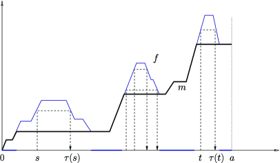
Figure 1: A schematic picture of the function $f$ and its backwards running minimum $m$, in bold. The set $C$ is marked bold on the abscissa, and instances of the mapping $t\mapsto\tau(t)$ are indicated by dashed lines.

We now fix $a\geq 0$ and decompose $f$ on $[0,a]$ according to its backwards running minimum $m$ given by

$$m(t)=\min\bigl{\{}f(s)\dvtx t\leq s\leq a\bigr{\}};$$

see Figure 1 for illustration. The nonnegative function $f-m$ can be decomposed on $[0,a]$ into a family $\mathcal{E}$ of excursions $e\dvtx[0,\infty)\to[0,\infty)$ with starting times $t_{e}\in[0,a]$. Note that an excursion $e\dvtx[0,\infty)\to[0,\infty)$ is a function such that there exists a number $\sigma_{e}>0$, called the lifetime of the excursion, such that $e(0)=0$, $e(s)>0$ for all $0<s<\sigma_{e}$, and $e(s)=0$ for all $s\geq\sigma_{e}$. Formally putting $e(s)=0$ for all $s<0$ the decomposition can be written as

$$f(t)-m(t)=\sum_{(e,t_{e})\in\mathcal{E}}e(t-t_{e}).$$

Note that the intervals $(t_{e},t_{e}+\sigma_{e})$, $(e,t_{e})\in\mathcal{E}$, are disjoint. We denote by $C$ the complement of their union in $[0,a]$, that is, $C=\{t\in[0,a]\dvtx f(t)=m(t)\}$.

Lemma 5.4

For every $(e,t_{e})\in\mathcal{E}$ we have

$$\xi\bigl{\{}s\in(t_{e},t_{e}+\sigma_{e})\dvtx\tau(s)\leq a\bigr{\}}=\xi(t_{e},t_{e}+\sigma_{e})=\eta(t_{e},t_{e}+\sigma_{e}).$$

We only have to show that $\tau(s)\leq a$ for $\xi$-almost every $s\in(t_{e},t_{e}+\sigma_{e})$. By Lemma 5.3(a), for $\xi$-almost every $s\in(t_{e},t_{e}+\sigma_{e})$, there exists $s_{n}\downarrow s$ such that $f(s_{n})>f(s)$. As $f(s)>f(t_{e}+\sigma_{e})$, by continuity of $f$, we infer that there exists $s^{*}\in(s,t_{e}+\sigma_{e})$ such that $f(s^{*})=f(s)$. Therefore $\tau(s)\leq s^{*}\leq a$ as required.

Lemma 5.5

We have

$$\xi\bigl{\{}s\in C\dvtx\tau(s)\leq a\bigr{\}}=\eta(C)=0.$$

First observe that if $s\in C$, then $f(t)\geq f(s)$ for all $t\in(s,a]$. If $f(t)>f(s)$ for all $t\in(s,a]$, then $\tau(s)>a$. Otherwise there exists a maximal $t\in(s,a]$ with $f(s)=f(t)$. Then $f(t)$ is a true local minimum of $f$ in the sense that there exists $r>0$ with $f(s)\geq f(t)$ for all $s\in(t-r,t)$ and $f(s)>f(t)$ for all $s\in(t,(t+r)\wedge a)$. In particular there are at most countably many levels $f(s)$ where this can happen. Fixing such a level $l$ we note that $\xi\{s\in C\dvtx f(s)=l\}=\eta\{s\in C\dvtx f(s)=l\}$. Summing over all these levels we see that $\xi\{s\in C\dvtx\tau(s)\leq a\}\leq\eta(C)$. We conclude the proof by showing that $\eta(C)=0$. Lemma 5.3(b) ensures that, for $\eta$-almost every $s\in[0,a]$ there exists $s_{n}\downarrow s$ such that $f(s_{n})<f(s)$, which implies that $s\notin C$. Hence the stated equality follows.

Proof of Lemma 5.2 Taking the sum over the equations in the previous two lemmas we obtain $\xi\{s\geq 0\dvtx\tau(s)\leq a\}=\eta[0,a]$. This implies

$$\int\mathbf{1}\bigl{\{}0\leq\tau(s)\leq a\bigr{\}}\xi(ds)=\eta[0,a],\qquad a\geq 0$$

as any $s<0$ with $f(s)<0$ satisfies $\tau(s)\notin[0,a]$, and Lemma 5.3(a) implies that $\xi$-almost every $s<0$ with $f(s)\geq 0$ satisfies $\tau(s)<0$, and so $\xi\{s<0\dvtx 0<\tau(s)\leq a\}=0$.

Proof of Theorem 5.1 Define

$$\xi^{\infty} := \int\mathbf{1}\bigl{\{}\tau(s)=\infty,s\in\cdot\bigr{\}}\xi(ds),$$

$$\eta^{*} := \int\mathbf{1}\bigl{\{}\tau(s)\in\cdot\bigr{\}}\xi(ds).$$

Recall that by Lemma 5.2 we have $\eta^{*}=\eta$ on $[s,\infty)$ provided $\xi[s,t]\geq\eta[s,t]$ for all $t\geq s$. By Lemma 5.3 this holds for $\xi^{\infty}$-a.e. $s$. Moreover, by invariance of $\xi^{\infty}$ and stationarity of $\mathbb{P}$ we have that $\mathbb{P}\{\xi^{\infty}(-\infty,s]=0,\xi^{\infty}\neq 0\}=0$ for all $s\in{\mathbb{R}}$. We infer that

$$\eta^{*}=\eta,\qquad\mbox{$\mathbb{P}$-a.e. on $\bigl{\{}\xi^{\infty}\neq 0\bigr{\}}$.}$$ (29)

Using the refined Campbell theorem (13) twice, we obtain

$$\mathbb{E}_{\mathbb{P}}\mathbf{1}\bigl{\{}\xi^{\infty}\neq 0\bigr{\}}\int_{0}^{1}\mathbf{1}\bigl{\{}\tau(s)<\infty\bigr{\}}\xi(ds)$$

$$\qquad=\mathbb{E}_{\mathbb{P}}\int_{0}^{1}\mathbf{1}\bigl{\{}\xi^{\infty}\circ\theta_{s}\neq 0,\tau(\theta_{s},0)<\infty\bigr{\}}\xi(ds)$$

$$\qquad=\mathbb{Q}_{\xi}\bigl{\{}\xi^{\infty}\neq 0,\tau(0)<\infty\bigr{\}}$$

(30)

$$\qquad=\mathbb{E}_{\mathbb{Q}_{\xi}}\int\mathbf{1}\bigl{\{}\xi^{\infty}\neq 0,\tau(0)+s\in[0,1]\bigr{\}}\,ds$$

$$\qquad=\mathbb{E}_{\mathbb{P}}\int\mathbf{1}\bigl{\{}\xi^{\infty}\neq 0,\tau(s)\in[0,1]\bigr{\}}\xi(ds)$$

$$\qquad=\mathbb{E}_{\mathbb{P}}\mathbf{1}\bigl{\{}\xi^{\infty}\neq 0\bigr{\}}\eta^{*}[0,1].$$

Using first (29) and then our assumption gives

$$\mathbb{E}_{\mathbb{P}}\mathbf{1}\bigl{\{}\xi^{\infty}\neq 0\bigr{\}}\eta^{*}[0,1]=\mathbb{E}_{\mathbb{P}}\mathbf{1}\bigl{\{}\xi^{\infty}\neq 0\bigr{\}}\eta[0,1]=\mathbb{E}_{\mathbb{P}}\mathbf{1}\bigl{\{}\xi^{\infty}\neq 0\bigr{\}}\xi[0,1],$$

and together with (5) we infer that

$$\mathbb{E}_{\mathbb{P}}\mathbf{1}\bigl{\{}\xi^{\infty}\neq 0\bigr{\}}\int_{0}^{1}\mathbf{1}\bigl{\{}\tau(s)<\infty\bigr{\}}\xi(ds)=\mathbb{E}_{\mathbb{P}}\mathbf{1}\bigl{\{}\xi^{\infty}\neq 0\bigr{\}}\xi[0,1],$$

and therefore $\tau(s)<\infty$ for $\xi$-a.e. $s$, $\mathbb{P}$-a.e. In particular, this implies that $\tau$ is a well-defined allocation rule. An analogous argument implies that

$$\tau^{-1}(s)>-\infty,\qquad\mbox{$\eta$-a.e. $s$, $\mathbb{P}$-a.e.},$$

where

$$\tau^{-1}(s)=\sup\bigl{\{}t<s\dvtx\xi[t,s]=\eta[t,s]\bigr{\}}$$

is the inverse of $\tau$. We now use this to show that $\tau$ balances $\xi$ and $\eta$. Fixing $a<b$ we aim to show that $\eta^{*}[a,b]=\eta[a,b]$. If $f(t)\geq f(a)$ for all $t\in[a,b]$, this holds by Lemma 5.2. Otherwise we apply this lemma to suitably chosen alternative intervals. To this end let

$$a^{*}:=\min\bigl{\{}s\in[a,b]\dvtx\mbox{$f(s)\leq f(t)$ for all $a\leq t\leq b$}\bigr{\}}$$

be the leftmost minimiser of $f$ on $[a,b]$. As $\eta(a^{*}-\frac{1}{n},a^{*}]\geq f(a^{*}-\frac{1}{n})-f(a^{*})>0$ for all sufficiently large $n\in{\mathbb{N}}$, we find a decreasing sequence $s_{n}$ with $\tau(s_{n})\downarrow a^{*}$ and hence $f(s_{n})\to f(a^{*})$. Then $s_{n}\downarrow s\in[-\infty,a]$ and $f(s)=f(a^{*})$ if $s\neq-\infty$.

Assuming first that $s\neq-\infty$, we obtain from Lemma 5.2 that

$$\int\mathbf{1}\bigl{\{}\tau(s)\in\cdot\bigr{\}}\xi(ds)=\eta(\cdot),\qquad\mbox{on $[s,b]$},$$

which implies the statement. Now assume that $s=-\infty$. In this case we get $\eta^{*}=\eta$ on $[s_{n},\tau(s_{n})]$ and on $[a^{*},b]$ for every $n$, and the result follows as $n\to\infty$.

The following is a counterpart of Theorem 5.1 for simple point processes.

Theorem 5.6

Let $\xi$ and $\eta$ be invariant simple point processes on ${\mathbb{R}}$ defined on some probability space equipped with a flow and an invariant $\sigma$-finite measure. Assume that $\xi$ and $\eta$ have finite intensities and that

$$\mathbb{E}_{\mathbb{P}}\bigl{[}\xi[0,1]\mid\mathcal{I}\bigr{]}=\mathbb{E}_{\mathbb{P}}\bigl{[}\eta[0,1]\mid\mathcal{I}\bigr{]}.$$

Then

$$\tau(s):=\inf\bigl{\{}t\geq s\dvtx\xi[s,t]=\eta[s,t]\bigr{\}},\qquad s\in{\mathbb{R}},$$ (31)

is an allocation rule balancing $\xi$ and $\eta$.

The allocation rule $\tau$ in Theorem 5.6 is a one-sided (and one-dimensional) version of the stable matching procedure described in HPPS09 . It can be proved by adapting the ideas of Theorem 5.1 to a discrete and therefore much simpler setup.

Theorem 5.1 implies the following result which contains Theorem 1.3 as a special case.

Theorem 5.7

Consider the Brownian case. If $\mu$ and $\nu$ are orthogonal probability measures on ${\mathbb{R}}$, then the stopping time

$$T^{\mu,\nu}:=\inf\bigl{\{}t>0\dvtx\ell^{\mu}[0,t]=\ell^{\nu}[0,t]\bigr{\}}$$ (32)

is an unbiased shift under $\mathbb{P}_{\mu}$ and $\mathbb{P}_{\mu}\{B_{T^{\mu,\nu}}\in\cdot\}=\nu$.

Theorem 3.5 implies that almost surely $\mathbb{E}_{\mathbb{P}}[\ell^{\mu}[0,1]|\mathcal{I}]=\break\mathbb{E}_{\mathbb{P}}[\ell^{\nu}[0,1]|\mathcal{I}]$. By assumption and (17) the invariant random measures $\ell^{\mu}$ and $\ell^{\nu}$ are orthogonal. Hence we can combine Theorems 5.1 and 4.1 to obtain the result.

Remark 5.8.

Assume in Theorem 1.3 that $\nu$ is a subprobability measure. Then $T$ takes the value $\infty$ with positive $\mathbb{P}_{0}$-probability. Indeed, by Remark 4.2, defining the extended allocation rule $\tau$ by $\tau(s):=s+T\circ\theta_{s}$ we get that $\tau$ balances the restriction of $\ell^{0}$ to $\{s\dvtx\tau(s)<\infty\}$ and $\ell^{\nu}$. Assertion (i) of Theorem 4.1 remains valid in the sense explained in Remark 4.2. The embedding property $\mathbb{P}_{0}\{T<\infty,B_{T}\in\cdot\}=\nu$ was proved in BertJan93 .

Remark 5.9.

Assume in Theorem 1.3 that $\nu$ is a locally finite measure with $\nu({\mathbb{R}})>1$ and $\nu\{0\}=0$. Then $\mathbb{P}_{0}\{T<\infty\}=1$ and $\tau$ balances $\ell^{0}$ and $\eta:=\int\mathbf{1}\{\tau(s)\in\cdot\}\ell^{0}(ds)$. The proof of Theorem 5.1 still yields the inequality $\eta\leq\ell^{\nu}$. In particular $\eta$ is a diffuse (and invariant) random measure with intensity $1$. The additive and continuous process $(A_{t})_{t\geq 0}$ given by $A_{t}:=\eta[0,t]$ is adapted to the filtration $(\sigma\{B_{s}\dvtx s\leq t\})_{t\geq 0}$. However, since Theorem 22.25 in Kallenberg applies only to one-sided Brownian motion, we cannot conclude that the process $(A_{t})_{t\geq 0}$ is of the form $(\ell^{\nu^{\prime}}[0,t])_{t\geq 0}$ for some probability measure $\nu^{\prime}$, and therefore it does not follow that the associated stopping time is an unbiased shift. The case $\nu=2\delta_{1}$ gives an example where it is easy to see that this may not be the case. Another example is discussed in Remark 5.10 below.

Remark 5.10.

In BertJan93 stopping times of the form discussed in Remark 5.9 are used to embed a given probability measure $\nu^{\prime}$ with $\int|x|\nu^{\prime}(dx)<\infty$ and $\nu^{\prime}\{0\}=0$. Indeed, as in BertJan93 , page 547, define $\rho(x):=2\int\mathbf{1}\{y>x\}(y-x)\nu^{\prime}(dy)$ for $x\geq 0$ and $\rho(x):=2\int\mathbf{1}\{y<x\}(x-y)\nu^{\prime}(dy)$ for $x<0$. Let $m_{0}$ be the maximum of the two numbers $2\int^{\infty}_{0}y\nu^{\prime}(dy)$ and $-2\int^{0}_{-\infty}y\nu^{\prime}(dy)$. It is proved in BertJan93 that

$$T:=\inf\biggl{\{}t>0\dvtx\ell^{0}[0,t]<m_{0}\int\ell^{x}[0,t]\rho^{-1}(x)\nu^{\prime}(dx)\biggr{\}}$$ (33)

embeds $\nu^{\prime}$ and satisfies $\mathbb{E}_{0}\ell^{0}[0,T]=m_{0}$. This $T$ is of the form (8) with $\nu({\mathbb{R}})>1$, provided that $\rho>0$ $\nu^{\prime}$-almost everywhere. This solution of the embedding problem is optimal in the sense that $\mathbb{E}_{0}\ell^{x}[0,S]\geq\mathbb{E}_{0}\ell^{x}[0,T]$, $x\in{\mathbb{R}}$, for any other stopping time $S\geq 0$ embedding $\nu^{\prime}$. The idea of using first passage times of additive functionals with infinite Revuz measures to embed probability distributions goes back to monroe72b . The fact that $\mathbb{E}_{0}\ell^{0}[0,T]<\infty$ reveals that $T$ cannot be an unbiased shift, as we show in Theorem 8.1 that this expectation is infinite for unbiased shifts.

The nonnegative unbiased shifts in Theorems 1.3, 1.4 and in 1.1 are all stopping times. In the next example we construct a nonnegative unbiased shift embedding a distribution not concentrated at zero, which is not a stopping time.

Example 5.11.

Let $x\in{\mathbb{R}}\setminus\{0\}$. We define an allocation rule $\tau$ that balances $\ell^{0}$ and $\ell^{x}$ and such that $T:=\tau(0)$ is nonnegative but not a stopping time. The mapping $\tau$ is the composition of the following five allocation rules. Let $\tau_{1}=\tau_{4}$ balance $\ell^{0}$ and $\ell^{x}$ according to Theorem 1.3. Let $\tau_{2}$ balance $\ell^{x}$ and $\ell^{x}$ by shifting forward one mass-unit, that is, let $\tau_{2}(0)$ be defined by (1) with $r=1$ and with $\ell^{0}$ replaced with $\ell^{x}$. Let $\tau_{3}$ balance $\ell^{x}$ and $\ell^{0}$ according to Theorem 1.3. Finally define $\tau_{5}$ by shifting backwards one mass-unit in the local time at $x$; that is, let $\tau_{5}$ be defined by (1) with $r=-1$ and $\ell^{0}$ replaced with $\ell^{x}$. The composition $\tau$ of these allocation rules balances $\ell^{0}$ and $\ell^{x}$. Moreover, $T:=\tau(0)\geq\tau_{1}(0)\geq 0$. However, $T$ is not a stopping time. This example can be extended to a general target distribution $\nu$.

6 Target distributions with an atom at zero

In this section we prove Theorems 1.4, 1.5, and 1.6. In contrast to the previous section we allow here for an atom at $0$.

Proof of Theorem 1.4 Let $y\in{\mathbb{R}}\setminus\{0\}$ such that $\nu\{y\}=0$, and define

$$\mu:=\nu-\nu\{0\}\delta_{0}+\nu\{0\}\delta_{y}.$$

Theorems 1.2 and 1.3 imply that the allocation rule

$$\tau^{\prime}(s):=\inf\bigl{\{}t>s\dvtx\ell^{0}[s,t]=\ell^{\mu}[s,t]\bigr{\}},\qquad s\in{\mathbb{R}},$$

balances $\ell^{0}$ and $\ell^{\mu}$. The same theorems imply that there is an allocation rule $\tau^{\prime\prime}$ that balances $\ell^{y}$ and $\ell^{0}$. Define

$$\tau(s):=\cases{\tau^{\prime}(s),&\quad$\mbox{if $B_{\tau^{\prime}(s)}\neq y$,}$\vspace*{2pt}\cr\tau^{\prime\prime}\bigl{(}\tau^{\prime}(s)\bigr{)},&\quad$\mbox{if $B_{\tau^{\prime}(s)}=y$}.$}$$

Then we have for any Borel set $C\subset{\mathbb{R}}$ outside a fixed $\mathbb{P}$-null set that

$$\int\mathbf{1}\bigl{\{}\tau(s)\in C\bigr{\}}\ell^{0}(ds)$$

$$\qquad=\int\mathbf{1}\bigl{\{}\tau(s)\in C,B_{\tau^{\prime}(s)}\neq y\bigr{\}}\ell^{0}(ds)$$

$$\qquad\quad{}+\int\mathbf{1}\bigl{\{}\tau(s)\in C,B_{\tau^{\prime}(s)}=y\bigr{\}}\ell^{0}(ds)$$

$$\qquad=\int\mathbf{1}\bigl{\{}\tau^{\prime}(s)\in C,B_{\tau^{\prime}(s)}\neq y\bigr{\}}\ell^{0}(ds)$$

$$\qquad\quad{}+\int\mathbf{1}\bigl{\{}\tau^{\prime\prime}\bigl{(}\tau^{\prime}(s)\bigr{)}\in C,B_{\tau^{\prime}(s)}=y\bigr{\}}\ell^{0}(ds)$$

$$\qquad=\int\mathbf{1}\{s\in C,B_{s}\neq y\}\ell^{\mu}(ds)+\int\mathbf{1}\bigl{\{}\tau^{\prime\prime}(s)\in C,B_{s}=y\bigr{\}}\ell^{\mu}(ds)$$

$$\qquad=\int\mathbf{1}\{x\neq 0\}\mathbf{1}\{s\in C\}\ell^{x}(ds)\nu(dx)+\nu\{0\}\int\mathbf{1}\bigl{\{}\tau^{\prime\prime}(s)\in C\bigr{\}}\ell^{y}(ds)$$

$$\qquad=\int\mathbf{1}\{x\neq 0\}\mathbf{1}\{s\in C\}\ell^{x}(ds)\nu(dx)+\nu\{0\}\ell^{0}(C)=\ell^{\nu}(C),$$

where we have used (17) (and $\nu\{y\}=0$) in the penultimate equation. Hence $\tau$ balances $\ell^{0}$ and $\ell^{\nu}$. Theorem 1.2 now implies that $T:=\tau(0)$ is an unbiased shift embedding $\nu$.

Proof of Theorem 1.5 Let $T$ be any unbiased shift embedding $\nu$ and define $\tau:=\tau_{T}$. Outside a fixed $\mathbb{P}$-null set we obtain for any Borel set $C\subset{\mathbb{R}}$ that

$$\int\mathbf{1}\bigl{\{}s\in C,\tau(s)=s\bigr{\}}\ell^{0}(ds) = \int\mathbf{1}\bigl{\{}\tau(s)\in C,\tau(s)=s\bigr{\}}\ell^{0}(ds)$$

$$= \int\mathbf{1}\bigl{\{}\tau(s)\in C,\tau(s)=s,B_{\tau(s)}=0\bigr{\}}\ell^{0}(ds)$$

$$\leq \int\mathbf{1}\bigl{\{}\tau(s)\in C,B_{\tau(s)}=0\bigr{\}}\ell^{0}(ds)$$

$$= \int\mathbf{1}\{s\in C,B_{s}=0\}\ell^{\nu}(ds)=\nu\{0\}\ell^{0}(C),$$

where we have used (17) to obtain the final identity. This implies that

$$\mathbf{1}\bigl{\{}\tau(s)=s\bigr{\}}\leq\nu\{0\},\qquad\mbox{$\ell^{0}$-a.e. $s$, $\mathbb{P}$-a.e.}$$

Assuming now that $\nu\{0\}<1$ we obtain $\tau(s)\neq s$ for $\ell^{0}$-a.e. $s$, $\mathbb{P}$-almost everywhere. Lemma 2.3 now implies (9).

Proof of Theorem 1.6 Let $\tau^{\prime}:=\tau_{T^{\prime}}$, where $T^{\prime}$ is given by (8) with $\nu=p\delta_{1}+(1-p)\delta_{2}$. Define an invariant random measure $\xi$ by $\xi(dt):=\mathbf{1}\{B_{\tau^{\prime}(t)}=2\}\ell^{0}(dt)$. The allocation rule

$$\tau^{\prime\prime}(s):=\inf\bigl{\{}t>s\dvtx\xi[s,t]=1\bigr{\}}$$

balances $\xi$ with itself. Define

$$\tau(s):=\cases{s,&\quad$\mbox{if $B_{\tau^{\prime}(s)}=1$,}$\vspace*{2pt}\cr\tau^{\prime\prime}(s),&\quad$\mbox{if $B_{\tau^{\prime}(s)}=2$}.$}$$

It is easy to see that $\tau$ balances $\ell^{0}$ with itself. Lemma 2.3 and Theorem 1.2 (or a direct calculation) implies that $T:=\tau(0)$ satisfies

$$\mathbb{P}_{0}\{T=0\}=\mathbb{P}_{0}\{B_{\tau^{\prime}(0)}=0\}=p.$$

Since $T$ is an unbiased shift, the proof is complete.

7 Stability and minimality of balancing allocations

We first work in the general setting of Section 2. The following definition is a one-sided version of the notion of stability introduced in HPPS09 for point processes. We call an allocation rule $\tau\dvtx\Omega\times{\mathbb{R}}\rightarrow{\mathbb{R}}$ balancing $\xi$ and $\eta$ right-stable if $\tau(s)\geq s$ for all $s\in{\mathbb{R}}$ and

$$\xi\otimes\xi\bigl{\{}(s,t)\dvtx t<s\leq\tau(t)<\tau(s)\bigr{\}}=0,\qquad\mathbb{P}\mbox{-a.e.}$$

Roughly speaking this means that the mass of pairs $(s,t)$ such that $s$ would prefer the partner of $t$ over its own partner, while $\tau(t)$ would prefer $s$ over $t$ as a partner, vanishes.

Theorem 7.1

Let $\xi$ and $\eta$ be invariant random measures satisfying the conditions of Theorem 5.1, and suppose $\tau\dvtx\Omega\times{\mathbb{R}}\rightarrow{\mathbb{R}}$ is the allocation rule constructed in the theorem. Then $\tau$ is right-stable.

By Lemma 5.3(a) and continuity of $f$, we have for $\xi$-a-e. $s$ that $f(s)<f(r)$ for all $r\in(s,\tau(s))$. Hence $\xi\otimes\xi$-almost every pair $(s,t)$ with $t<s\leq\tau(t)<\tau(s)$ satisfies $f(t)<f(s)<f(\tau(t))$ contradicting the definition of $\tau$.

Right-stable allocation rules have a useful minimality property.

Theorem 7.2

Any right-stable allocation rule $\tau$ balancing two measures $\xi$ and $\eta$ is minimal in the sense that if $\sigma$ is another allocation rule balancing $\xi$ and $\eta$ such that $s\leq\sigma(s)\leq\tau(s)$ for $\xi$-almost every $s\in{\mathbb{R}}$, then $\xi\{s\dvtx\sigma(s)<\tau(s)\}=0$.

By right-stability of $\tau$ we have, for $\xi$-almost every $a$,

$$s\in\bigl{[}a,\tau(a)\bigr{]}\quad\Longleftrightarrow\quad\tau(s)\in\bigl{[}a,\tau(a)\bigr{]},\qquad\xi\mbox{-a.e. $s$}.$$ (34)

From the assumption $s\leq\sigma(s)\leq\tau(s)$ and (34) we obtain for any $t\in[a,\tau(a)]$ that $\tau(s)\in[a,t]$ implies $\sigma(s)\in[a,t]$ for $\xi$-almost every $s$. Therefore

$$\eta[a,t]=\int\mathbf{1}\bigl{\{}\tau(s)\in[a,t]\bigr{\}}\xi(ds)\leq\int\mathbf{1}\bigl{\{}\sigma(s)\in[a,t]\bigr{\}}\xi(ds)=\eta[a,t].$$

This implies

$$\mathbf{1}\bigl{\{}\tau(s)\in[a,t]\bigr{\}}=\mathbf{1}\bigl{\{}\sigma(s)\in[a,t]\bigr{\}},\qquad\xi\mbox{-a.e. $s\in{\mathbb{R}}$}.$$

Therefore $\tau$ and $\sigma$ coincide $\xi$-almost everywhere on $\tau^{-1}([a,\tau(a)])$.

Now fix some $b\in{\mathbb{R}}$ and recall the definition of the backwards running minimum $m(t)=\min\{f(s)\dvtx t\leq s\leq b\}$ and the set $C=\{t\leq b\dvtx m(t)=f(t)\}$. We have seen that the complement of $C$ consists of countably many intervals $(a,\tau(a))$ as above and therefore $\tau$ and $\sigma$ coincide $\xi$-almost everywhere on $\tau^{-1}((-\infty,b]\setminus C)$. On the other hand, by Lemma 5.5 we have $\xi(\tau^{-1}(C))=\eta(C)=0$, as required to finish the argument.

Remark 7.3.

In the point process case the allocation rule (31) is right-stable, and it is not difficult to show that it is the unique right-stable allocation balancing $\xi$ and $\eta$. We conjecture that this uniqueness property also holds in the general case and therefore can be added to Theorem 7.1.

Remark 7.4.

One could define an allocation rule $\tau$ to be stable if

$$\xi\otimes\xi\bigl{\{}(s,t)\dvtx\bigl{|}s-\tau(t)\bigr{|}<\bigl{|}s-\tau(s)\bigr{|},\bigl{|}s-\tau(t)\bigr{|}<\bigl{|}t-\tau(t)\bigr{|}\bigr{\}}=0.$$

The rule $\tau$ of Theorem 5.1 does not satisfy this. We do not know if stable allocation rules in the above sense exist, or if they are unique.

In the remainder of this section we consider the Brownian case. An unbiased shift $T$ is called minimal unbiased shift if $\mathbb{P}_{0}\{T\geq 0\}=1$ and if any other unbiased shift $S$ such that $\mathbb{P}_{0}\{0\leq S\leq T\}=1$ and $\mathbb{P}_{0}\{B_{T}\in\cdot\}=\mathbb{P}_{0}\{B_{S}\in\cdot\}$ satisfies $\mathbb{P}_{0}\{S=T\}=1$. The following theorem provides more insight into the set of all minimal unbiased shifts. The result and its proof are motivated by Proposition 2 in monroe72 .

Theorem 7.5

Let $T$ be an unbiased shift embedding the probability measure $\nu$ and such that $\mathbb{P}_{0}\{T\geq 0\}=1$. Then there exists a minimal unbiased shift $T^{*}$ embedding $\nu$ and such that $\mathbb{P}_{0}\{0\leq T^{*}\leq T\}=1$.

Let $\mathcal{T}$ denote the set of all unbiased shifts $S$ embedding $\nu$ and such that $\mathbb{P}_{0}\{0\leq S\leq T\}=1$. This is a partially ordered set, where we do not distinguish between elements that coincide $\mathbb{P}_{0}$-a.s. By the Hausdorff maximal principle (see, e.g., Dudley , Section 1.5) there is a maximal chain $\mathcal{T}^{\prime}\subset\mathcal{T}$. This is a totally ordered set that is not contained in a strictly bigger totally ordered set. Let

$$\alpha:=\sup_{S\in\mathcal{T}^{\prime}}\mathbb{E}_{0}e^{-S}.$$

Then there is a sequence $S_{n}$, $n\in{\mathbb{N}}$, such that $\mathbb{E}_{0}e^{-S_{n}}\to\alpha$ as $n\to\infty$. Since $\mathcal{T}^{\prime}$ is totally ordered, it is no restriction of generality to assume that the $S_{n}$ are decreasing $\mathbb{P}_{0}$-a.s. Define $T^{*}:=\lim_{n\to\infty}S_{n}$. By construction and monotone convergence,

$$\mathbb{E}_{0}e^{-T^{*}}=\alpha.$$ (35)

We also note that $\mathbb{P}_{0}\{0\leq T^{*}\leq T\}=1$.

We claim that $T^{*}$ is a minimal unbiased shift embedding $\nu$ and first show that $T^{*}$ is an unbiased shift. Let $k\in{\mathbb{N}}$, and consider continuous and bounded functions $f\dvtx{\mathbb{R}}^{k}\rightarrow{\mathbb{R}}$ and $g\dvtx{\mathbb{R}}\rightarrow{\mathbb{R}}$. Let $t_{1},\dots,t_{k}\in{\mathbb{R}}$. Since $S_{n}\in\mathcal{T}$ for any $n\in{\mathbb{N}}$, we have that

$$\mathbb{E}_{0}f(B_{S_{n}+t_{1}}-B_{S_{n}},\dots,B_{S_{n}+t_{k}}-B_{S_{n}})g(B_{S_{n}})$$

(36)

$$\qquad=\mathbb{E}_{0}f(B_{t_{1}},\dots,B_{t_{k}})\int g(x)\nu(dx).$$

By bounded convergence the above left-hand side converges toward

$$\mathbb{E}_{0}f(B_{T^{*}+t_{1}}-B_{T^{*}},\dots,B_{T^{*}+t_{k}}-B_{T^{*}})g(B_{T^{*}})$$

as $n\to\infty$. The monotone class theorem implies that $T^{*}$ is an unbiased shift embedding $\nu$.

It remains to show the minimality property of $T^{*}$. Assume on the contrary that there is some unbiased shift $S$ embedding $\nu$ such that $\mathbb{P}_{0}\{0\leq S\leq T^{*}\}=1$ and $\mathbb{P}_{0}\{S<T^{*}\}>0$. The last two relations imply that

$$\mathbb{E}_{0}e^{-S}>\mathbb{E}_{0}e^{-T^{*}}.$$

By (35) this means that $S\notin\mathcal{T}^{\prime}$. On the other hand, since $\mathbb{P}_{0}\{S\leq T^{*}\leq T\}=1$, we have that $S\in\mathcal{T}$, contradicting the maximality property of $\mathcal{T}^{\prime}$.

As announced in the Introduction the stopping time $T^{\nu}$ is a minimal unbiased shift:

Theorem 7.6

Let $\nu$ be a probability measure on ${\mathbb{R}}$ with $\nu\{0\}=0$. Then $T^{\nu}$ defined by (8) is a minimal unbiased shift.

Let $S$ be an unbiased shift embedding $\nu$ and such that $\mathbb{P}_{0}\{0\leq S\leq T^{\nu}\}~{}=~{}1$. Theorem 1.2 implies that the allocation rules $\tau_{S}$ and $\tau_{T^{\nu}}$ balance $\ell^{0}$ and $\ell^{\nu}$. By Theorem 7.1, $\tau_{T^{\nu}}$ is right-stable $\mathbb{P}$-a.e. The assumptions yield $\ell^{0}\{s\dvtx s\leq\tau_{S}(s)\leq\tau_{T^{\nu}}(s)\}=0$ $\mathbb{P}$-a.e. By Theorem 7.2 we therefore have $\ell^{0}\{s\dvtx\tau_{S}(s)<\tau_{T^{\nu}}(s)\}=0$ $\mathbb{P}$-a.e. This readily implies that $\mathbb{P}_{0}\{S=T^{\nu}\}=1$.

8 Moments of unbiased shifts

In this section we consider the Brownian case and discuss moment properties of unbiased shifts. The following two theorems together were stated as Theorem 1.7 in the Introduction.

Theorem 8.1

Suppose $\nu$ is a target distribution with $\nu\{0\}=0$, and the stopping time $T\geq 0$ is an unbiased shift embedding $\nu$. Then

$$\mathbb{E}_{0}T^{1/4}=\infty.$$

We start the proof with a reminder of the Barlow–Yor inequality BY , which states that, for any $p>0$ there exist constants $0<c<C$ such that, for all stopping times $T$,

$$c\mathbb{E}_{0}T^{p/2}\leq\mathbb{E}_{0}\sup_{x}\ell^{x}[0,T]^{p}\leq C\mathbb{E}_{0}T^{p/2}.$$

Hence it suffices to verify that $\mathbb{E}_{0}\ell^{0}[0,T]^{1/2}=\infty$.

The proof of this fact uses an argument similar to that in the proof of Theorem 2 in HPPS09 . Let $\tau=\tau_{T}$ be the allocation rule associated with $T$, and set $T_{r}=\sup\{s\geq 0\dvtx\ell^{0}[0,s]=r\}$ for $r>0$, as at (1). Then, on the one hand,

$$\mathbb{E}_{0}\int\mathbf{1}\bigl{\{}0\leq s\leq T_{r},\tau(s)\notin[0,T_{r}]\bigr{\}}\ell^{0}(ds)$$

$$\qquad=\mathbb{E}_{0}\int^{T_{r}}_{0}\mathbf{1}\bigl{\{}\tau(s)-s>T_{r}-s\bigr{\}}\ell^{0}(ds)$$

$$\qquad=\int^{r}_{0}\mathbb{P}_{0}\bigl{\{}\tau(T_{s})-T_{s}>T_{r}-T_{s}\bigr{\}}\,ds=\int^{r}_{0}\mathbb{P}_{0}\{T\circ\theta_{T_{s}}>T_{r-s}\circ\theta_{T_{s}}\}\,ds$$

$$\qquad=\int^{r}_{0}\mathbb{P}_{0}\{T>T_{s}\}\,ds=\mathbb{E}_{0}\bigl{[}\ell^{0}[0,T]\wedge r\bigr{]},$$

where we have used the strong Markov property at $T_{s}$ (or Theorem 1.1) for the fourth step and change of variable for the second and fifth steps. On the other hand, the fact that $\tau$ balances $\ell^{0}$ and $\ell^{\nu}$ easily implies that

$$\int\mathbf{1}\bigl{\{}0\leq s\leq T_{r},\tau(s)\notin[0,T_{r}]\bigr{\}}\ell^{0}(ds)\geq\bigl{(}\ell^{0}[0,T_{r}]-\ell^{\nu}[0,T_{r}]\bigr{)}_{+}.$$

Hence, combining these two facts with the obvious fact that $\ell^{0}[0,T_{r}]=r$, we get

$$\mathbb{E}_{0}\bigl{[}\ell^{0}[0,T]\wedge r\bigr{]}\geq\mathbb{E}_{0}\bigl{(}r-\ell^{\nu}[0,T_{r}]\bigr{)}_{+}.$$ (37)

We now show that

$$\liminf_{r\to\infty}r^{-1/2}\mathbb{E}_{0}\bigl{(}r-\ell^{\nu}[0,T_{r}]\bigr{)}_{+}>0.$$ (38)

To this end we apply a concentration inequality of Petrov for arbitrary sums of independent random variables; see Petrov95 , Theorem 2.22. It shows that there exists a constant $C>0$ such that, for all $\varepsilon>0$ and $r\geq 1$,

$$\mathbb{P}\bigl{\{}\ell^{\nu}[0,T_{r}]\in[r-\varepsilon\sqrt{r},r+\varepsilon\sqrt{r}]\bigr{\}}\leq C\varepsilon.$$

Now observe that $\mathbb{E}_{0}\ell^{\nu}[0,T_{r}]=r$, which is an immediate consequence of the second Ray–Knight theorem (see Theorem 2.3 in Chapter XI of RevYor99 ) but can also be derived from general Palm theory. Hence, by Markov’s inequality,

$$\mathbb{E}_{0}\bigl{(}r-\ell^{\nu}[0,T_{r}]\bigr{)}_{+} = \tfrac 12\mathbb{E}_{0}\bigl{|}r-\ell^{\nu}[0,T_{r}]\bigr{|}\geq\tfrac 12\varepsilon\sqrt{r}\mathbb{P}\bigl{\{}\bigl{|}r-\ell^{\nu}[0,T_{r}]\bigr{|}>\varepsilon\sqrt{r}\bigr{\}}$$

$$\geq \tfrac 12\varepsilon(1-C\varepsilon)\sqrt{r}$$

as required to prove (38). Combining (37) and (38) gives

$$\liminf_{r\to\infty}r^{-1/2}\mathbb{E}_{0}\bigl{[}\ell^{0}[0,T]\wedge r\bigr{]}>0.$$

Finally, assume for contradiction that $\mathbb{E}_{0}[\ell^{0}[0,T]^{1/2}]<\infty$. Since$r^{-1/2}(\ell^{0}[0,T]\wedge r)\leq\ell^{0}[0,T]^{1/2}$, dominated convergence implies that$r^{-1/2}\mathbb{E}_{0}[\ell^{0}[0,T]\wedge r]\to 0$ as $r\to\infty$, which is in contradiction to the last display.

Note that the unbiased shifts $T^{\nu}$ satisfy the conditions of Theorem 8.1 if $\nu$ has finite mean. The next result shows that they have nearly optimal moment properties.

Theorem 8.2

Let $\nu$ satisfy $\int|x|\nu(dx)<\infty$, and let $T=T^{\nu}$ be the stopping time constructed in (8). Then, for all $\beta\in[0,1/4)$,

$$\mathbb{E}_{0}T^{\beta}<\infty.$$ (39)

The proof of Theorem 8.2 uses a result similar to Theorem 4(ii) in HP05 and Theorem 2 in HPPS09 , which is of independent interest and may also serve as another example for Theorem 5.1. We consider the “clock”

$$U_{r}:=\inf\bigl{\{}t>0\dvtx\ell^{0}[0,t]+\ell^{\nu}[0,t]=r\bigr{\}}$$

and random measures $\xi$ and $\eta$ on the positive reals given by

$$\xi[0,r]:=\ell^{0}[0,U_{r}],\qquad\eta[0,r]:=\ell^{\nu}[0,U_{r}],\qquad r\geq 0.$$

Proposition 8.3

Let $\xi$ and $\eta$ be defined as above, and let $S:=\inf\{t>0\dvtx\xi[0,t]=\eta[0,t]\}$. Then $\mathbb{E}_{0}S^{1/2}=\infty$, but for some $c>0$ we have $\mathbb{P}_{0}\{S>t\}\leq ct^{-1/2}$, for all $t\in{\mathbb{R}}$.

The proof of $\mathbb{E}_{0}S^{1/2}=\infty$ is very similar to Theorem 2 in HPPS09 and is therefore omitted. We prove here the upper bound for the tail asymptotics (only this part is needed). This result is similar to Theorem 6(ii) in HPPS09 , but due to the specific form of $S$ we can use a more direct argument.

For any $i\in{\mathbb{N}}$ let $Y_{i}=\eta\{s\geq 0\dvtx i-1<\xi[0,s]\leq i\}$. As in the proof of Theorem 8.1 the second Ray–Knight theorem implies that $Y_{i}$ has mean one. Together with Jensen’s inequality we get

$$\qquad\mathbb{E}_{0}\bigl{[}Y_{i}^{2}\bigr{]}=\mathbb{E}_{0}\bigl{(}\ell^{\nu}[0,T_{1}]\bigr{)}^{2}\leq\mathbb{E}_{0}\int\bigl{(}\ell^{x}[0,T_{1}]\bigr{)}^{2}\nu(dx)=\int\bigl{(}1+|x|\bigr{)}\nu(dx),$$ (40)

which is finite by assumption. Summarising, the sequence $Y_{1},Y_{2},\ldots$ is an i.i.d. sequence of random variables with mean one and finite variance. Define, for $n\in{\mathbb{N}}$,

$$R_{n}:=\sum_{i=1}^{n}1+Y_{i},\qquad U_{n}:=\sum_{i=1}^{n}1-Y_{i}.$$

Let $\sigma:=\inf\{n\geq 1\dvtx U_{n}<0\}$, and fix $a\in(0,1/2)$. Then, for any $t>0$,

$$\mathbb{P}_{0}\{S>t\}\leq\mathbb{P}_{0}\{R_{\sigma}>t\}\leq\mathbb{P}_{0}\{\mbox{$U_{n}\geq 0$ for all $n\leq at$}\}+\mathbb{P}_{0}\{R_{\lfloor at\rfloor}>t\}.$$

By a classical result of Spitzer Spitzer60 , see also Feller , Theorem 1a in Section XII.7, the first term on the above right-hand side is bounded by a constant multiple of $(at)^{-1/2}$. By Chebyshev’s inequality, we have

$$\mathbb{P}_{0}\{R_{\lfloor at\rfloor}>t\}\leq\frac{1}{\bigl{(}t-2\lfloor at\rfloor\bigr{)}^{2}}\mathbb{E}_{0}\bigl{[}\bigl{(}R_{\lfloor at\rfloor}-2\lfloor at\rfloor\bigr{)}^{2}\bigr{]}=\frac{\lfloor at\rfloor}{(t-2\lfloor at\rfloor)^{2}}\mathbb{E}_{0}\bigl{[}(1-Y_{1})^{2}\bigr{]},$$

which is bounded by a constant multiple of $t^{-1}$. This completes the proof.

Proof of Theorem 8.2 The variable $S$, defined in Proposition 8.3, satisfies

$$S=\ell^{0}[0,T]+\ell^{\nu}[0,T]=2\ell^{0}[0,T].$$

It remains to relate the tail behaviour of $\ell^{0}[0,T]$ (which we know) to that of $T$ (which we require). To this end we observe that for $\theta\in{\mathbb{R}}$ and $t>\frac{3}{4}$, using MortersPeres , Theorem 6.10,

$$\mathbb{P}_{0}\biggl{\{}\inf_{s>t}\frac{1}{\sqrt{s/\log s}}\ell^{0}[0,s]<1/\theta\biggr{\}}$$

$$\qquad=\mathbb{P}_{0}\biggl{\{}\inf_{s>t}\frac{1}{\sqrt{s/\log s}}\max_{0\leq r\leq s}|B_{r}|<1/\theta\biggr{\}}$$

$$\qquad\leq\sum_{k=0}^{\infty}\mathbb{P}_{0}\biggl{\{}\frac{1}{\sqrt{t+k}}\max_{0\leq r\leq t+k}|B_{r}|<\frac{2}{\theta\sqrt{\log(t+k)}}\biggr{\}}.$$

By a step in the proof of Chung’s law of the iterated logarithm (see, e.g., JP75 , equation (2.1)),

$$\mathbb{P}_{0}\biggl{\{}\frac{1}{\sqrt{t}}\max_{0\leq r\leq t}|B_{r}|<x\biggr{\}}\leq\frac{4}{\pi}e^{-{\pi^{2}}/{(8x^{2})}},\qquad x>0,$$

and hence we have

$$\mathbb{P}_{0}\biggl{\{}\inf_{s>t}\frac{1}{\sqrt{s/\log s}}\ell^{0}[0,s]<1/\theta\biggr{\}}\leq t^{-1/4}$$

for a sufficiently large constant $\theta$. For sufficiently large $t$ we have

$$\mathbb{P}_{0}\biggl{\{}\frac{T}{\theta^{2}\log T}>t\biggr{\}}\leq\mathbb{P}_{0}\bigl{\{}\ell^{0}[0,T]>\sqrt{t}\bigr{\}}+\mathbb{P}_{0}\biggl{\{}\inf_{s>t}\frac{1}{\sqrt{s/\log s}}\ell^{0}[0,s]<1/\theta\biggr{\}},$$

and the right-hand side in this inequality is bounded by a constant multiple of $t^{-1/4}$. The result follows directly by integration.

Next we turn to unbiased shifts $T$ embedding a measure $\nu\neq\delta_{0}$, which need neither be stopping times, nor nonnegative. We conjecture that any such shift satisfies $\mathbb{E}_{0}|T|^{1/4}=\infty$. At the moment we can only prove the following weaker result.

Theorem 8.4

If $T$ is an unbiased shift embedding a probability measure $\nu\neq\delta_{0}$, then

$$\mathbb{E}_{0}\sqrt{|T|}=\infty.$$

The idea of this proof is due to Alex Cox. We work under the probability measure $\mathbb{P}_{0}$. By definition of an unbiased shift $B^{+}:=(B_{T+t}-B_{T}\dvtx t\geq 0)$ and $B^{-}:=(B_{T-t}-B_{T}\dvtx t\geq 0)$ are independent Brownian motions. Moreover, the pair $(B^{+},B^{-})$ is independent of $B_{T}$. Assume that $B_{T}\geq x$, where $x>0$ is chosen such that $\nu[x,\infty)>0$. (If there is no such $x>0$ we find an $x<0$ such that $\nu(-\infty,x]>0$ and assume $B_{T}\leq x$.) If $T>0$, then $B^{-}_{T}=-B_{T}\leq-x$, so that

$$T\geq S^{-}:=\inf\bigl{\{}t\geq 0\dvtx B^{-}_{t}=-x\bigr{\}}.$$

If $T<0$, then $B^{+}_{-T}=-B^{-}_{T}\leq-x$, so that

$$-T\geq S^{+}:=\inf\bigl{\{}t\geq 0\dvtx B^{+}_{t}=-x\bigr{\}}.$$

Hence $|T|\geq S^{-}\wedge S^{+}=:S$. It is well known that $\mathbb{E}_{0}\sqrt{S^{-}}=\infty$ and $\mathbb{E}_{0}\sqrt{S^{+}}=\infty$. Since $S^{-}$ and $S^{+}$ are independent, this property transfers to $S$. It follows that

$$\mathbb{E}_{0}\sqrt{|T|}\geq\mathbb{E}_{0}\mathbf{1}\{B_{T}\geq x\}\sqrt{S}=\nu[x,\infty)\mathbb{E}_{0}\sqrt{S}=\infty.$$ (41)

Unbiased shifts embedding $\delta_{0}$ also have bad moment properties if they are nonnegative (or, by time-reversal, nonpositive) but not identically zero. The result can be compared with Theorem 3(i) in HPPS09 . However, the proofs are very different.

Theorem 8.5

If $T\geq 0$ is an unbiased shift such that $\mathbb{P}_{0}\{B_{T}=0\}=1$ and $\mathbb{P}_{0}\{T>0\}>0$, then

$$\mathbb{E}_{0}T=\infty.$$

We assume for contradiction that $m:=\mathbb{E}_{0}T<\infty$. Define a probability measure $\mathbb{P}^{*}$ on $\Omega$ by setting $\mathbb{E}_{\mathbb{P}^{*}}f(B)=\frac{1}{m}\mathbb{E}_{0}\int_{0}^{T}f(\theta_{s}B)\,ds$ for each bounded nonnegative measurable function $f$. By Lemma 3.2, $\mathbb{P}^{*}$ is stationary. To show that, on the invariant $\sigma$-algebra $\mathcal{I}$, the process $B$ has the same distribution under $\mathbb{P}^{*}$ as under $\mathbb{P}_{0}$, take $A\in\mathcal{I}$ and recall from Theorem 3.5 that $\mathbb{P}_{0}\{B\in A\}\in\{0,1\}$. But $\mathbb{P}^{*}\{B\in A\}=\frac{1}{m}\mathbb{E}_{0}\mathbf{1}\{B\in A\}T=0$ or $1$ according as $\mathbb{P}_{0}\{B\in A\}=0$ or $1$, as required. By Thor96 , Theorem 2, we infer from this that

$$\frac{1}{t}\int_{0}^{t}\mathbb{P}_{0}\{\theta_{s}B\in\cdot\}\,ds\to\mathbb{P}^{*}\{B\in\cdot\},\qquad t\to\infty,$$

with respect to the total variation norm. On the other hand, for every $r>0$,

$$\frac{1}{t}\int_{0}^{t}\mathbb{P}_{0}\bigl{\{}|B_{s}|\leq r\bigr{\}}\,ds\to 0,\qquad t\to\infty,$$

implying $\mathbb{P}^{*}\{|B_{0}|\leq r\}=0$ for all $r>0$, which is a contradiction.

In contrast to the two theorems above, we shall see below that unbiased shifts can have good moment properties if they can assume both signs.

Example 8.6.

We construct a nonzero unbiased shift $T$ embedding $\delta_{0}$, which has $\mathbb{E}e^{\lambda|T|}<\infty$ for some $\lambda>0$. Let $\{(a_{i},b_{i})\dvtx i\in{\mathbb{Z}}\}$ be the countable collection of maximal nonempty intervals $(a,b)$ with the property that $B_{t}\neq 0$ for all $a<t<b$ and $|B_{s}|\geq 1$ for some $s\in(a,b)$. We assume that the collection is ordered such that $b_{i}<a_{i+1}$ for all $i\in{\mathbb{Z}}$. We define an allocation rule $\tau$ by the requirement that, for $b_{i}<s<a_{i+1}$,

$$\tau(s)=\cases{\sup\bigl{\{}r<a_{i+1}\dvtx\ell^{0}(r,a_{i+1})=\ell^{0}(b_{i},s)\bigr{\}},&\quad$\mbox{if $\ell^{0}(b_{i},s)\leq\frac{1}{2}\ell^{0}(b_{i},a_{i+1})$},$\vspace*{2pt}\cr\inf\bigl{\{}r>b_{i}\dvtx\ell^{0}(s,a_{i+1})=\ell^{0}(b_{i},r)\bigr{\}},&\quad$\mbox{if $\ell^{0}(b_{i},s)>\frac{1}{2}\ell^{0}(b_{i},a_{i+1})$}.$}$$

It is easy to see that $\tau$ balances $\ell^{0}$ with itself, and hence by Theorem 1.2, we have that $T=\tau(0)$ is an unbiased shift embedding $\delta_{0}$. Moreover, we have $|T|\leq S_{1}+S_{2}$ where $S_{1}=\inf\{t>0\dvtx|B_{t}|=1\}$ and $S_{2}=-\sup\{t<0\dvtx\break|B_{t}|=1\}$. $S_{1}$ and $S_{2}$ are obviously independent and identically distributed, and it is easy to see that they, and hence $|T|$, have the required moment property.

Remark 8.7.

If $T\geq 0$ is an unbiased shift such that $\mathbb{P}_{0}\{B_{T}=0\}=1$ and $\mathbb{P}_{0}\{T>0\}>0$, then we conjecture that $\mathbb{E}_{0}\sqrt{T}=\infty$ (strengthening Theorem 8.5), but we cannot prove this without additional assumptions. One such assumption [covering $T_{r}$ defined in (1) for $r>0$] is that $\mathbb{P}_{0}\{T>s\}>0$ for some $s>0$ such that $\{T>s\}$ is $\mathbb{P}_{0}$-almost surely in the $\sigma$-algebra generated by $\{B_{t}\dvtx t\leq s\}$. Indeed, in this case we have

$$\mathbb{E}_{0}\sqrt{|T|}\geq\mathbb{E}_{0}\mathbf{1}\{T>s\}\sqrt{T}\geq\mathbb{E}_{0}\mathbf{1}\{T>s\}\sqrt{s+T_{0}\circ\theta_{s}},$$

where $T_{0}:=\inf\{t>0\dvtx B_{t}=0\}$. By the Markov property

$$\mathbb{E}_{0}\sqrt{|T|}\geq\mathbb{E}_{0}\mathbf{1}\{T>s\}\mathbb{E}_{B_{s}}\sqrt{T_{0}}=\infty,$$

since $\mathbb{E}_{x}\sqrt{T_{0}}=\infty$ for all $x\neq 0$ and $\mathbb{P}_{0}\{B_{s}=0\}=0$. Note that this argument does not use that $T$ is unbiased.

9 Unbiased shifts of Lévy processes

In this section we extend some of our previous results to a larger class of Lévy processes. A Lévy process is a right-continuous real-valued stochastic process $X=(X_{t})_{t\in{\mathbb{R}}}$ with left-hand limits and $X_{0}=0$, having independent and stationary increments; see, for example, Bert02 , Kallenberg . In particular the (left-continuous) process $(X_{-t})_{t\geq 0}$ is independent of $X^{+}:=(X_{t})_{t\geq 0}$ and has the same finite-dimensional distributions as $-X^{+}$. We assume that $X$ is recurrent; see Bert02 for a definition.

For convenience, we also assume that $X$ is given as the identity on its canonical space $(\Omega,\mathcal{A},\mathbb{P}_{0})$, where $\Omega$ is the set of all right-continuous functions $\omega\dvtx{\mathbb{R}}\rightarrow{\mathbb{R}}$ with left-hand limits and $\mathcal{A}$ is the Kolmogorov product $\sigma$-algebra. As in the Brownian case we define $\mathbb{P}_{x}:=\mathbb{P}_{0}\{X+x\in\cdot\}$, $x\in{\mathbb{R}}$, and $\mathbb{P}$ by (2). This $\mathbb{P}$ has the stationarity property (10), where the shifts are defined by (3). This setting is a special case of the one established in Section 2.

The Lévy–Khinchine formula states that

$$\mathbb{E}_{0}e^{i\vartheta X_{t}}=e^{-t\psi(\vartheta)},\qquad t\geq 0,$$ (42)

where

$$\psi(\vartheta)=ia\vartheta+\frac{\sigma^{2}\vartheta^{2}}{2}+\int\bigl{(}1-e^{i\vartheta x}+i\vartheta x\mathbf{1}\bigl{\{}|x|\leq 1\bigr{\}}\bigr{)}\Pi(dx),\qquad\vartheta\in{\mathbb{R}}.$$

Here $a\in{\mathbb{R}}$, $\sigma^{2}\geq 0$ and the Lévy measure $\Pi$ satisfies $\Pi\{0\}=0$ and $\int x^{2}\wedge 1\Pi(dx)<\infty$. We assume that, first,

$$\int\Re\biggl{(}\frac{1}{u+\psi(\vartheta)}\biggr{)}\,d\vartheta<\infty,\qquad u>0,$$

which means that points are not essentially polar, and, second, that either $\sigma^{2}>0$ or $\int|x|\wedge 1\Pi(dx)=\infty$, which means that the Lévy process is of unbounded variation. These two assumptions imply that the origin is regular for itself; see Theorem 8 in Bret71 . Theorem 4 in GeKe72 then implies that there are random (local time) measures $\ell^{x}$, $x\in{\mathbb{R}}$, such that $(\omega,x)\mapsto\ell^{x}(\omega,C)$ is measurable for all Borel sets $C\subset{\mathbb{R}}$, and (14) holds. Moreover, $\ell^{x}$ is $\mathbb{P}_{0}$-a.s. diffuse for any $x\in{\mathbb{R}}$. In order to apply the techniques of this paper we need a perfect version of local times satisfying (15), (16), and (17). To achieve this we assume the conditions $(R_{\beta})$ and $(H)$ of BPT86 , Theorem 1.2. We do not formulate these (somewhat technical) assumptions here, but only mention that they are satisfied by a strictly $\alpha$-stable Lévy process, whenever $\alpha>1$. [The case $\alpha=2$ corresponds to Brownian motion while for $\alpha<2$ the Lévy measure is given by $\Pi(dx)=c_{+}x^{-\alpha-1}\,dx$ on $(0,\infty)$ and $\Pi(dx)=c_{-}|x|^{-\alpha-1}\,dx$ on $(-\infty,0)$.]

As in the Brownian case we define for any locally finite measure $\mu$ on ${\mathbb{R}}$ the invariant random measure $\ell^{\mu}$ by (6). If $\mu$ is a probability measure, then we call a random time $T$ an unbiased shift under $\mathbb{P}_{\mu}:=\int\mathbb{P}_{x}\mu(dx)$ if $(X_{T+t}-X_{T})_{t\in{\mathbb{R}}}$ is independent of $X_{T}$ and has distribution $\mathbb{P}_{0}$ under $\mathbb{P}_{\mu}$.

Theorem 9.1

Let $T$ be a random time and $\mu,\nu$ be probability measures on ${\mathbb{R}}$. Then $T$ is an unbiased shift under $\mathbb{P}_{\mu}$ and $\mathbb{P}_{\mu}\{X_{T}\in\cdot\}=\nu$ if and only if the allocation rule $\tau_{T}$ defined by (7) balances $\ell^{\mu}$ and $\ell^{\nu}$.

The proof of Lemma 2.3 yields that $\mathbb{P}_{x}$ is the Palm measure of $\ell^{x}$ with respect to $\mathbb{P}$. Therefore $\mathbb{P}_{\mu}$ is the Palm measure of $\ell^{\mu}$, and the proof of Theorem 4.1 applies without change.

Theorem 9.2

Let $\mu$ be a probability measure on ${\mathbb{R}}$, and let $S_{r}$, $r\in{\mathbb{R}}$, be the generalised inverse of $\ell^{\mu}$ defined as in (1). Then $S_{r}$ is an unbiased shift under $\mathbb{P}_{\mu}$ and $\mathbb{P}_{\mu}\{X_{S_{r}}\in\cdot\}=\mu$.

In order to apply Theorem 3.1 we need to show that $\mathbb{P}_{\mu}\{\ell^{\mu}(0,\break\infty)<\infty\}=0$. Since the Lévy process $-X$ also satisfies our general assumptions, this implies $\mathbb{P}_{\mu}\{\ell^{\mu}(-\infty,0)<\infty\}=0$. Clearly, it is enough to prove $\mathbb{P}_{x}\{\ell^{y}(0,\infty)<\infty\}=0$ for all $x,y\in{\mathbb{R}}$. By the spatial homogeneity (16) this is equivalent to

$$\mathbb{P}_{0}\bigl{\{}\ell^{x}(0,\infty)<\infty\bigr{\}}=0,\qquad x\in{\mathbb{R}}.$$ (43)

By Proposition V.4 in Bert02 the generalised inverse of $(\ell^{0}[0,t])_{t\geq 0}$ is (under $\mathbb{P}_{0}$) a (finite) subordinator, so that (43) holds for $x=0$. Spatial homogeneity implies that $\mathbb{P}_{x}\{\ell^{x}(0,\infty)<\infty\}=0$. As the origin is regular for itself, the results in Bert02 , Chapter II (see in particular Theorems II.16 and II.19) imply that our process is not only recurrent, but that the origin is point-recurrent and that $T^{\prime}_{x}:=\inf\{t\geq 0\dvtx X_{t}=x\}$ is finite $\mathbb{P}_{0}$-a.s. Hence (43) follows from the strong Markov property applied to $T^{\prime}_{x}$, which is a stopping time with respect to a suitable augmentation of the natural filtration.

Theorem 9.3

Let $A\in\mathcal{I}$ be a shift-invariant set. Then either $\mathbb{P}_{x}(A)=0$ for all $x\in{\mathbb{R}}$ or $\mathbb{P}_{x}(A^{c})=0$ for all $x\in{\mathbb{R}}$.

The proof of Theorem 3.5 applies provided that $\mathbb{P}_{0}\{\ell^{x}\neq 0\}=1$ for $\lambda$-a.e. $x\in{\mathbb{R}}$. But this follows from (43).

Thanks to Theorem 5.1 the previous result implies the following generalisation of Theorem 5.7.

Theorem 9.4

Let $\mu$ and $\nu$ be orthogonal probability measures on ${\mathbb{R}}$. Then the stopping time $T:=T^{\mu,\nu}$ defined by (32) is an unbiased shift under $\mathbb{P}_{\mu}$ and $\mathbb{P}_{\mu}\{X_{T}\in\cdot\}=\nu$.

Theorems 1.4, 1.5 and 1.6 as well as the minimality properties stated in Theorems 7.5 and 7.6 do also hold in the present, more general setting. It would be interesting to study the moment properties of unbiased shifts of Lévy processes. The proof of Theorem 1.7 makes significant use of the properties of Brownian motion. Theorem 8.5, however, is still true in the Lévy case while the proof of Theorem 8.4 can be extended beyond the Brownian case.

References

- (1) {barticle}[mr] \bauthor\bsnmBarlow, \bfnmMartin T.\binitsM. T., \bauthor\bsnmPerkins, \bfnmEdwin A.\binitsE. A. and \bauthor\bsnmTaylor, \bfnmS. James\binitsS. J. (\byear1986). \btitleTwo uniform intrinsic constructions for the local time of a class of Lévy processes. \bjournalIllinois J. Math. \bvolume30 \bpages19–65. \bidissn=0019-2082, mr=0822383 \bptokimsref \endbibitem
- (2) {barticle}[mr] \bauthor\bsnmBarlow, \bfnmM. T.\binitsM. T. and \bauthor\bsnmYor, \bfnmM.\binitsM. (\byear1981). \btitle(Semi-) martingale inequalities and local times. \bjournalZ. Wahrsch. Verw. Gebiete \bvolume55 \bpages237–254. \biddoi=10.1007/BF00532117, issn=0044-3719, mr=0608019 \bptokimsref \endbibitem
- (3) {bbook}[mr] \bauthor\bsnmBertoin, \bfnmJean\binitsJ. (\byear1996). \btitleLévy Processes. \bseriesCambridge Tracts in Mathematics \bvolume121. \bpublisherCambridge Univ. Press, \blocationCambridge. \bidmr=1406564 \bptnotecheck year\bptokimsref \endbibitem
- (4) {barticle}[mr] \bauthor\bsnmBertoin, \bfnmJ.\binitsJ. and \bauthor\bsnmLe Jan, \bfnmY.\binitsY. (\byear1992). \btitleRepresentation of measures by balayage from a regular recurrent point. \bjournalAnn. Probab. \bvolume20 \bpages538–548. \bidissn=0091-1798, mr=1143434 \bptokimsref \endbibitem
- (5) {bincollection}[mr] \bauthor\bsnmBretagnolle, \bfnmJean\binitsJ. (\byear1971). \btitleRésultats de Kesten sur les processus à accroissements indépendants. In \bbooktitleSéminaire de Probabilités, V (Univ. Strasbourg, Année Universitaire 1969–1970). \bseriesLecture Notes in Math. \bvolume191 \bpages21–36. \bpublisherSpringer, \blocationBerlin. \bidmr=0368175 \bptokimsref \endbibitem
- (6) {barticle}[mr] \bauthor\bsnmCox, \bfnmA. M. G.\binitsA. M. G. and \bauthor\bsnmHobson, \bfnmD. G.\binitsD. G. (\byear2006). \btitleSkorokhod embeddings, minimality and non-centred target distributions. \bjournalProbab. Theory Related Fields \bvolume135 \bpages395–414. \biddoi=10.1007/s00440-005-0467-y, issn=0178-8051, mr=2240692 \bptokimsref \endbibitem
- (7) {bbook}[mr] \bauthor\bsnmDudley, \bfnmR. M.\binitsR. M. (\byear2002). \btitleReal Analysis and Probability. \bseriesCambridge Studies in Advanced Mathematics \bvolume74. \bpublisherCambridge Univ. Press, \blocationCambridge. \biddoi=10.1017/CBO9780511755347, mr=1932358 \bptnotecheck year\bptokimsref \endbibitem
- (8) {bbook}[mr] \bauthor\bsnmFeller, \bfnmWilliam\binitsW. (\byear1971). \btitleAn Introduction to Probability Theory and Its Applications. Vol. II., \bedition2nd ed. \bpublisherWiley, \blocationNew York. \bidmr=0270403 \bptnotecheck year\bptokimsref \endbibitem
- (9) {barticle}[mr] \bauthor\bsnmGeman, \bfnmD.\binitsD. and \bauthor\bsnmHorowitz, \bfnmJ.\binitsJ. (\byear1973). \btitleOccupation times for smooth stationary processes. \bjournalAnn. Probab. \bvolume1 \bpages131–137. \bidmr=0350833 \bptokimsref \endbibitem
- (10) {barticle}[mr] \bauthor\bsnmGetoor, \bfnmR. K.\binitsR. K. and \bauthor\bsnmKesten, \bfnmH.\binitsH. (\byear1972). \btitleContinuity of local times for Markov processes. \bjournalCompos. Math. \bvolume24 \bpages277–303. \bidissn=0010-437X, mr=0310977 \bptokimsref \endbibitem
- (11) {barticle}[mr] \bauthor\bsnmHolroyd, \bfnmAlexander E.\binitsA. E., \bauthor\bsnmPemantle, \bfnmRobin\binitsR., \bauthor\bsnmPeres, \bfnmYuval\binitsY. and \bauthor\bsnmSchramm, \bfnmOded\binitsO. (\byear2009). \btitlePoisson matching. \bjournalAnn. Inst. Henri Poincaré Probab. Stat. \bvolume45 \bpages266–287. \biddoi=10.1214/08-AIHP170, issn=0246-0203, mr=2500239 \bptokimsref \endbibitem
- (12) {barticle}[mr] \bauthor\bsnmHolroyd, \bfnmAlexander E.\binitsA. E. and \bauthor\bsnmPeres, \bfnmYuval\binitsY. (\byear2005). \btitleExtra heads and invariant allocations. \bjournalAnn. Probab. \bvolume33 \bpages31–52. \biddoi=10.1214/009117904000000603, issn=0091-1798, mr=2118858 \bptokimsref \endbibitem
- (13) {barticle}[mr] \bauthor\bsnmJain, \bfnmNaresh C.\binitsN. C. and \bauthor\bsnmPruitt, \bfnmWilliam E.\binitsW. E. (\byear1975). \btitleThe other law of the iterated logarithm. \bjournalAnn. Probab. \bvolume3 \bpages1046–1049. \bidmr=0397845 \bptokimsref \endbibitem
- (14) {bincollection}[auto] \bauthor\bsnmKagan, \bfnmY. A.\binitsY. A. and \bauthor\bsnmVere-Jones, \bfnmD.\binitsD. (\byear1996). \btitleAthens Conference on Applied Probability and Time Series Analysis. Vol. I, (\beditor\binitsC. C.\bfnmC. C. \bsnmHeyde, \beditor\binitsY. V.\bfnmY. V. \bsnmProhorov, \beditor\binitsR.\bfnmR. \bsnmPyke and \beditor\binitsS. T.\bfnmS. T. \bsnmRachev, eds.). \bseriesLecture Notes in Statistics \bvolume114. \bpublisherSpringer, \blocationNew York. \biddoi=10.1007/978-1-4612-0749-8, mr=1466703 \bptokimsref \endbibitem
- (15) {bbook}[mr] \bauthor\bsnmKallenberg, \bfnmOlav\binitsO. (\byear2002). \btitleFoundations of Modern Probability, \bedition2nd ed. \bpublisherSpringer, \blocationNew York. \bidmr=1876169 \bptokimsref \endbibitem
- (16) {bincollection}[mr] \bauthor\bsnmLast, \bfnmGünter\binitsG. (\byear2010). \btitleModern random measures: Palm theory and related models. In \bbooktitleNew Perspectives in Stochastic Geometry (\beditor\bfnmW.\binitsW. \bsnmKendall and \beditor\bfnmI.\binitsI. \bsnmMolchanov, eds.) \bpages77–110. \bpublisherOxford Univ. Press, \blocationOxford. \bidmr=2654676 \bptokimsref \endbibitem
- (17) {barticle}[mr] \bauthor\bsnmLast, \bfnmGünter\binitsG. and \bauthor\bsnmThorisson, \bfnmHermann\binitsH. (\byear2009). \btitleInvariant transports of stationary random measures and mass-stationarity. \bjournalAnn. Probab. \bvolume37 \bpages790–813. \biddoi=10.1214/08-AOP420, issn=0091-1798, mr=2510024 \bptokimsref \endbibitem
- (18) {bincollection}[mr] \bauthor\bsnmLiggett, \bfnmThomas M.\binitsT. M. (\byear2002). \btitleTagged particle distributions or how to choose a head at random. In \bbooktitleIn and Out of Equilibrium (Mambucaba, 2000) (\beditor\bfnmV.\binitsV. \bsnmSidoravicius, ed.). \bseriesProgress in Probability \bvolume51 \bpages133–162. \bpublisherBirkhäuser, \blocationBoston, MA. \bidmr=1901951 \bptokimsref \endbibitem
- (19) {bbook}[mr] \bauthor\bsnmMandelbrot, \bfnmBenoit B.\binitsB. B. (\byear1982). \btitleThe Fractal Geometry of Nature. \bpublisherW. H. Freeman and Co., \blocationSan Francisco, CA. \bidmr=0665254 \bptokimsref \endbibitem
- (20) {barticle}[mr] \bauthor\bsnmMecke, \bfnmJ.\binitsJ. (\byear1967). \btitleStationäre zufällige Maße auf lokalkompakten Abelschen Gruppen. \bjournalZ. Wahrsch. Verw. Gebiete \bvolume9 \bpages36–58. \bidmr=0228027 \bptokimsref \endbibitem
- (21) {barticle}[mr] \bauthor\bsnmMonroe, \bfnmItrel\binitsI. (\byear1972). \btitleOn embedding right continuous martingales in Brownian motion. \bjournalAnn. Math. Statist. \bvolume43 \bpages1293–1311. \bidissn=0003-4851, mr=0343354 \bptokimsref \endbibitem
- (22) {barticle}[mr] \bauthor\bsnmMonroe, \bfnmItrel\binitsI. (\byear1972). \btitleUsing additive functionals to embed preassigned distributions in symmetric stable processes. \bjournalTrans. Amer. Math. Soc. \bvolume163 \bpages131–146. \bidissn=0002-9947, mr=0298768 \bptokimsref \endbibitem
- (23) {bbook}[mr] \bauthor\bsnmMörters, \bfnmPeter\binitsP. and \bauthor\bsnmPeres, \bfnmYuval\binitsY. (\byear2010). \btitleBrownian Motion. \bpublisherCambridge Univ. Press, \blocationCambridge. \bidmr=2604525 \bptokimsref \endbibitem
- (24) {barticle}[mr] \bauthor\bsnmObłój, \bfnmJan\binitsJ. (\byear2004). \btitleThe Skorokhod embedding problem and its offspring. \bjournalProbab. Surv. \bvolume1 \bpages321–390. \biddoi=10.1214/154957804100000060, issn=1549-5787, mr=2068476 \bptokimsref \endbibitem
- (25) {barticle}[mr] \bauthor\bsnmPerkins, \bfnmEdwin\binitsE. (\byear1981). \btitleA global intrinsic characterization of Brownian local time. \bjournalAnn. Probab. \bvolume9 \bpages800–817. \bidissn=0091-1798, mr=0628874 \bptokimsref \endbibitem
- (26) {bbook}[mr] \bauthor\bsnmPetrov, \bfnmValentin V.\binitsV. V. (\byear1995). \btitleLimit Theorems of Probability Theory: Sequences of Independent Random Variables. \bseriesOxford Studies in Probability \bvolume4. \bpublisherOxford Univ. Press, \blocationNew York. \bidmr=1353441 \bptokimsref \endbibitem
- (27) {bbook}[mr] \bauthor\bsnmRevuz, \bfnmDaniel\binitsD. and \bauthor\bsnmYor, \bfnmMarc\binitsM. (\byear1999). \btitleContinuous Martingales and Brownian Motion, \bedition3rd ed. \bseriesGrundlehren der Mathematischen Wissenschaften \bvolume293. \bpublisherSpringer, \blocationBerlin. \bidmr=1725357 \bptokimsref \endbibitem
- (28) {barticle}[mr] \bauthor\bsnmSpitzer, \bfnmFrank\binitsF. (\byear1960). \btitleA Tauberian theorem and its probability interpretation. \bjournalTrans. Amer. Math. Soc. \bvolume94 \bpages150–169. \bidissn=0002-9947, mr=0111066 \bptokimsref \endbibitem
- (29) {barticle}[mr] \bauthor\bsnmThorisson, \bfnmHermann\binitsH. (\byear1996). \btitleTransforming random elements and shifting random fields. \bjournalAnn. Probab. \bvolume24 \bpages2057–2064. \biddoi=10.1214/aop/1041903217, issn=0091-1798, mr=1415240 \bptokimsref \endbibitem
- (30) {bbook}[mr] \bauthor\bsnmThorisson, \bfnmHermann\binitsH. (\byear2000). \btitleCoupling, Stationarity, and Regeneration. \bpublisherSpringer, \blocationNew York. \biddoi=10.1007/978-1-4612-1236-2, mr=1741181 \bptokimsref \endbibitem
- (31) {barticle}[mr] \bauthor\bsnmZähle, \bfnmU.\binitsU. (\byear1991). \btitleSelf-similar random measures. III. Self-similar random processes. \bjournalMath. Nachr. \bvolume151 \bpages121–148. \biddoi=10.1002/mana.19911510110, issn=0025-584X, mr=1121202 \bptokimsref \endbibitem