Energy transfer dynamics and thermalization of two oscillators interacting via chaos

Abstract

We consider the classical dynamics of two particles moving in harmonic potential wells and interacting with the same external environment $H_{E}$, consisting of $N$ non-interacting chaotic systems. The parameters are set so that when either particle is separately placed in contact with the environment, a dissipative behavior is observed. When both particles are simultaneously in contact with $H_{E}$ an indirect coupling between them is observed only if the particles are in near resonance. We study the equilibrium properties of the system considering ensemble averages for the case $N=1$ and single trajectory dynamics for $N$ large. In both cases, the particles and the environment reach an equilibrium configuration at long times, but only for large $N$ a temperature can be assigned to the system.

I Introduction

Understanding dissipation from a microscopic point of view has become important to several areas of physics, especially if quantum phenomena are relevant. In these cases a globally conservative approach for the system plus its environment is highly desirable, allowing a direct quantum mechanical description.

The simplest, and perhaps most natural, way to model the environment is to use an infinite set of harmonic oscillators, representing the normal modes of a general system in equilibrium weakly perturbed by the system of interest caldeira83 ; caldeira . The spectral function, which is related to the distribution of frequencies of the normal modes, can be chosen to model several types of thermal baths fisher85 ; weiss93 ; hedegard87 . Other representations of the environment have also been explored, from spin systems prokofiev00 (or two-level atoms) to chaotic systems Wilkinson (1990); berry93 ; tulio ; Cohen (1999); cohen1 . The latter is particularly important to model coupling to small external systems where the chaotic nature of the trajectories compensates for the small number of degrees of freedom in the decay of correlation functions. However, chaos alone does not suffice to simulate a thermal bath, since small numbers of degrees of freedom always leave a strong signature in the dynamics through large fluctuations in the observables of the system of interest Marchiori and de Aguiar (2011). These fluctuations can be washed out by averaging over several realizations of the dynamics Bonanca and de Aguiar (2006).

More recently, the interest has shifted from a single particle interacting with the environment to two particles independently connected to it dua06 ; dua09 ; val10 , allowing the study of interactions mediated by the environment. One important case is that of two entangled particles subjected to dissipation and decoherence. In many cases, the total Hamiltonian is symmetric by the exchange of the particles, although they may still be considered distinguishable in some applications dua06 .

In this paper we consider the classical dynamics of two particles moving in harmonic potentials linearly coupled to a finite chaotic environment. We study the system behavior as a function of the frequency of the oscillators. We find that the behavior of the system changes radically when the oscillators are in resonance, which is a necessary condition if the particles are identical, and that even small deviations from this symmetric state changes dramatically the equilibrium properties of the system. In particular, we show that, when in resonance, the particles may exchange energy through the environment while their energies dissipate. Moreover, the energy stored in their relative motion is conserved.

We model the environment as a set of $N$ independent quartic systems (QS), each with 2 degrees of freedom. The QS has a single parameter that controls the degree of chaos in the dynamics. The particles are represented by two harmonic oscillators independently coupled to the set of QS’s. As study cases we consider the systems with $N=1$ and $N=100$, for which we study the statistical properties of the energy distributions of the environment and of the oscillators. In both cases, these distributions reach an asymptotic equilibrium, but attempts to define a temperature for the system using two basic definitions of entropy, applicable to small systems, succeed only in the case $N=100$. The results of the simulations are then interpreted in the light of the linear response theory.

II Model

We consider two harmonic oscillators interacting with an environment composed by a collection of independent quartic systems. The Hamiltonian is

$$H=H_{1}+H_{2}+H_{E}+\lambda_{N}H_{I},$$ (1)

where $\lambda_{N}=\lambda/\sqrt{N}$ and

$$H_{i} = \frac{p^{2}_{i}}{2m_{i}}+\frac{m_{i}\omega_{i}^{2}q_{i}^{2}}{2},\quad i=1,2,$$ (2)

$$H_{E} = \sum_{n=1}^{N}\left[\frac{p_{x_{n}}^{2}+p_{y_{n}}^{2}}{2}+\frac{a}{4}(x_{n}^{4}+y_{n}^{4})+\frac{x_{n}^{2}y_{n}^{2}}{2}\right]\equiv\sum_{n=1}^{N}H_{QS}^{(n)},$$ (3)

$$H_{I} = \sum_{n=1}^{N}(q_{1}+q_{2})\,x_{n}.$$ (4)

The total energy is conserved and the two oscillators interact only via the environment.

In our simulations, we used $\lambda=0.01$. The parameter $a$ in $H_{QS}$ controls the dynamical regime of the quartic systems in the environment, ranging from integrable (for the special values $a=1.0$ and $a=0.33$ joy93 ) to chaotic ($a\rightarrow 0$). In the work, we used $a=0.01$ or $a=0.1$, which correspond to regimes where the QS is mostly chaotic. For $a=0.1$ the largest Lyapunov exponent of an isolated QS is $\lambda_{L}=0.166$ for energy $E_{QS}=0.1$. For $a=0.01$ we obtained $\lambda_{L}=0.121$ for $E_{QS}=0.01$. Because of the scaling properties of the QS, the Lyapunov exponent at other energies can be calculated using $\lambda_{L}(E)=(E/E_{0})^{1/4}\lambda_{L}(E_{0})$.

As the number of degrees of freedom is finite, the parameter $N$ assumes a prominent role and we investigate its influence in the dynamic behavior of the oscillators. It has been recently shown Marchiori and de Aguiar (2011) that, for $N$ sufficiently large, such finite chaotic environment can simulate the action of an infinite thermal reservoir. Here the environment also acts as a medium connecting the two harmonic oscillators.

In order to highlight the interaction between the oscillators, one of them is initialized with energy $E_{1}>0$ while the other is set at rest with $E_{2}=0$. For the environment we define the initial conditions using the pseudo canonical distribution Marchiori and de Aguiar (2011)

$$\rho=\frac{1}{Z}\prod_{n=1}^{N}\delta(H_{QS}^{(n)}-E_{QS}^{(n)}),$$ (5)

where the energy $E_{QS}^{(n)}$ of each QS is randomly chosen from the exponential probability distribution $\exp{(-E/\bar{E}_{QS})}/\bar{E}_{QS}$. The value of $\bar{E}_{QS}$ plays the role of an initial “temperature” for the environment. In the special case of $N=1$ the energy $E_{QS}$ is fixed to $\bar{E}_{QS}$.

In what follows we will study the system (1) for only two relevant environment sizes: the “microscopic” ($N=1$) and “macroscopic” ($N=100$) cases. As pointed out in Marchiori and de Aguiar (2011), the dynamical behavior of the system becomes $N$-independent for $N$ sufficiently large. For the parameters values used in this paper, the large $N$ limit is already reached for $N=100$. The case $N=1$ is a natural extension of the work presented in Bonanca and de Aguiar (2006), where the authors considered the interaction between a harmonic oscillator and a single quartic system using ensemble averages. Thence we choose the same set of parameters as in Bonanca and de Aguiar (2006) in our simulations, allowing us to verify the implications of adding a second oscillator to the system. For $N=100$, on the other hand, we compare our results with the work presented in Marchiori and de Aguiar (2011), which treated the dynamics of a single oscillator interacting with large chaotic environments.

In the microscopic case, observables related to the harmonic oscillators, like the energies $H_{1}$ or $H_{2}$, exhibit large fluctuations when coupled to $H_{QS}$. These fluctuations can only be washed out by averaging over large ensembles of realizations of the dynamics. In the macroscopic case this is not necessary and the results obtained from a single realization of the dynamics are already representative of the average behavior. In this case we can speak of an “effective dynamics”, where no averages are performed.

III Measures of temperature

Temperature is a central property in the description of equilibrium and is properly defined only in the thermodynamic limit of very large systems. Since the environment defined in Eq. (3) is far from this limit for $N=1$ and $N=100$, different possibilities arise. One natural definition comes from the equipartition theorem rt1918

$$\Big{\langle}z_{m}\frac{\partial H}{\partial z_{n}}\Big{\rangle}=\delta_{mn}\tau_{E},$$ (6)

where $z_{n}$ denotes the coordinates or momenta of the system and $\delta_{mn}$ is the Kronecker delta. The constant $\tau_{E}$ is identified with $k_{B}T$ when the system is in contact with a thermal reservoir. The subscript in $\tau_{E}$ emphasizes the explicit use of the equipartition theorem. Eqs. (1) and (6) predict that the fraction of the total energy within each subsystem in equilibrium should be $\langle E_{1}\rangle=\langle E_{2}\rangle=\tau_{E}=2/3\langle E_{QS}\rangle$. We can also write the system’s temperature as a function of the number of quartic systems as

$$E_{T}=E_{1}(0)+E_{2}(0)+E^{T}_{QS}(0)=2\tau_{E}+\frac{3}{2}N\tau_{E},$$ (7)

in which $E^{T}_{QS}(0)$ is the environment’s total energy at $t=0$.

Eq. (7) can also be derived from the thermodynamic relation be91

$$\tau_{E}^{-1}=\frac{\partial\ln{\Gamma}}{\partial E_{T}},$$ (8)

where

$$\Gamma(E_{T})=\int\Theta(E_{T}-H)\mspace{1.0mu}dp\mspace{1.0mu}dq$$ (9)

and the integral is taken over the entire phase space of the system. For the Hamiltonian in Eq. (1) we obtain

$$\Gamma=c\,E_{T}^{3N_{f}/4+2},$$ (10)

where $N_{f}=2N$ is the number of degrees of freedom of the environment and $c$ represents a constant depending on the system parameters.

Notice that

$$\ln{\Gamma}=\ln{c}+(3N_{f}/4+2)\ln{E_{T}}$$ (11)

plays the role of entropy. The usual entropy, on the other hand, is given by

$$S(E) = \ln{\left[\int\delta(E-H)\mspace{1.0mu}dp\mspace{1.0mu}dq\right]}=\ln{\frac{\partial\Gamma}{\partial E}}$$ (12)

$$= \ln{c}+(3N_{f}/4+1)\ln{E}+\ln{(3N_{f}/4+2)}.$$

Defining $\tau_{S}^{-1}=\partial S(E_{T})/\partial E_{T}$ we obtain

$$E_{T}=\tau_{S}+\frac{3}{2}N\tau_{S},$$ (13)

which agrees with (7) in the limit of large $N$.

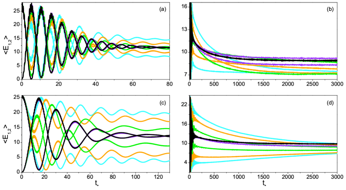
Figure 1: (Color online) Short- and long-time energy dynamics of the oscillators at various values of $k=0$ (black), $1$ (purple), $6$ (green), $11$ (orange), $16$ (cyan) for energies of $E_{QS\mspace{-1.7mu}}(0)=0.1$ (panels (a) and (b)) and $E_{QS\mspace{-1.7mu}}(0)=5$ (panels (c) and (d)). The averages were computed using an ensemble of $40000$ initial conditions. Colors change gradually from light gray to black as the $k$ value decreases, if printed in black and white.

The two temperatures, $\tau_{E}$ and $\tau_{S}$, can be calculated numerically in a number of ways. According to ru97 , $\tau_{S}$ may be calculated from the dynamics using the expression ru97 ; jep00

$$\tau_{S}^{d}={\langle\Phi(H)\rangle}^{-1},$$ (14)

where $\tau_{S}^{d}/k_{B}$ is the so-called Rugh’s temperature and

$$\Phi(H)\equiv\text{div}\mspace{4.0mu}\frac{\nabla H}{\lVert\nabla H\rVert{}^{2}}$$ (15)

with $\nabla$ denoting the gradient in phase space. This formula assumes that the energy, $H=E$, is the only isolating integral. On the other hand, $\tau_{E}$ can be estimated as a dynamical average, as in the left hand side of Eq. (6). We use the superscript $d$ to emphasize that these temperatures are obtained from the dynamics, i.e., from the trajectories.

Finally, the temperature can be calculated from fitting the energy distribution $p(E)$, which is the probability of finding one QS with energy $E$ when the system is in equilibrium, as the Boltzmann exponential $p_{B}(E)\sim\exp{\mspace{-1.0mu}(-E/\tau_{B})}$. Another possibility is to numerically calculate the distribution of momentum and fit it with the Maxwellian profile $p_{M}(p)\sim\exp{\mspace{-1.0mu}(-p^{2}/(2m\tau_{M}))}$. These distributions will be obtained from the numerical data for the oscillators and will be used to check the predictions arising from Eqs. (7) and (13).

In the limit of large systems, we expect all these measures to approach the same equilibrium value; however, for small number of degrees of freedom, they are likely to differ vb98 . We will use two basic definitions of temperature, and the different ways to calculate them, to assess the equilibrium properties of our model system.

IV Dynamics via ensemble average ($N=1$)

In this section, we investigate the approach to equilibrium and equipartition of energy for the system described by the Hamiltonian (1) with only one quartic system, which means $N=1$. We examine, particularly, the energy transfer dynamics of this system for cases in which the coupling between the subsystems is weak and the harmonic oscillators are near-to-resonance. We test for equilibration by comparing the calculated distributions of energy and momentum with appropriate equilibrium distributions. We also analyze and compare the dynamical behavior of $\tau_{E}^{d}$ with that of $\tau_{S}^{d}$, concentrating on the issue of energy equipartition between the energy stored in the oscillators and in the quartic system at large times.

Our approach makes use of averaging over large ensembles of different initial chaotic configurations that have a common fixed energy shell where $H_{QS}=E_{QS}$. The initial conditions for the two harmonic oscillators are $q_{1}=0$, $p_{1}=\sqrt{\smash[b]{2m_{1}E_{1\mspace{-2.0mu}}(0)}}$, $q_{2}=0$, and $p_{2}=\sqrt{\smash[b]{2m_{2}E_{2\mspace{-2.0mu}}(0)}}$. The initial data used for the phase space variables $x,y,p_{x},p_{y}$ originate from points along a single trajectory of the uncoupled chaotic quartic system, rather than from random starting points in an energy shell.

To solve numerically the equations of motion, we used the fourth-order Runge-Kutta method (detailed for example in gg89 ). The integration time step length was set to ensure energy conservation to within $1\%$ for each individual trajectory. The ensemble average value of an observable is calculated as the mean of its estimates generated by propagating initial conditions in the ensemble. Throughout this section, we set $m_{1}=m_{2}=10$ and $a=0.1$ Bonanca and de Aguiar (2006).

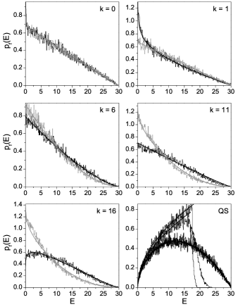
Figure 2: Distributions of energy for the three subsystems at time $t_{\text{f}}$, computed with initial value $E_{QS}=5$. The ragged black curves in each $k$-labeled panel are for oscillator 1; the gray curves are for oscillator 2, and the smooth curves are plotted according to Eq. (16). The bottom-right panel displays results for QS, with $k$ increasing from top curve to bottom curve.

The left panels in Fig. 1 present the short-time energy transfer dynamics between the two harmonic oscillators. Their average energies are plotted versus dimensionless time $t_{*}=\omega_{1}t/2\pi$ for the initial energies $E_{QS}=0.1$ (panel (a)) and $E_{QS}=5$ (panel (c)), and frequencies $\omega_{2}$ in a small deviation from the frequency $\omega_{1}=0.0125$: $\omega_{2}=\omega_{1}+k\,\Delta$, with fixed value $\Delta=0.0000375$ for $k=\{0,1,6,11,16\}$. The initial energies of the oscillators are chosen as $E_{1}=25$ and $E_{2}=0$. It is readily seen that the energy curves for $k=0$ and $1$ are almost identical for both situations; however the response to $E_{QS}=0.1$ is faster than that of $E_{QS}=5$. Another important feature is the appreciably less energy transferred from one oscillator to the other at greater $k$ values.

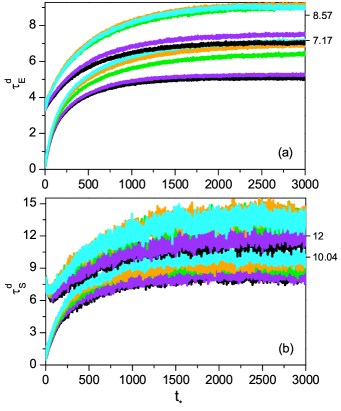
Figure 3: (Color online) Panel (a): time evolution of $\langle p_{x}^{2}\rangle$ for $E_{QS\mspace{-1.7mu}}(0)=0.1$ (bottom curves) and $E_{QS\mspace{-1.7mu}}(0)=5$ (top curves). Panel (b): time evolution of $\tau_{S}^{d}$ for $E_{QS\mspace{-1.7mu}}(0)=0.1$ (bottom curves) and $E_{QS\mspace{-1.7mu}}(0)=5$ (top curves). Colors and parameters as in Fig. 1, except that, for the calculation of $\tau_{S}^{d}$, $4000$ initial conditions were used instead of $40000$. The results for $\langle p_{y}^{2}\rangle$ are nearly identical to those of $\langle p_{x}^{2}\rangle$.

The right panels of Fig. 1 in turn capture the long-time behavior of the average energies of the two oscillators under $E_{QS}=0.1$ (panel (b)) and $E_{QS}=5$ (panel (d)) conditions. Except for the case when the frequencies coincide, the final energies for the oscillators are visibly different for each initial state of the system. These panels indicate that the equilibration time is very long and might not be reached in practical situations. Not shown here is the behavior of the chaotic system’s average energy, which ascends gradually with time and more rapidly with increasing $k$, approaching a saturation value. See panel (a) in Fig. 3 for a plot of $\langle p_{x}^{2}\rangle$ as a function of $t_{*}$.

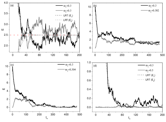
Figure 4: (Color online) Energy of the oscillators as a function of the scaled time $t_{*}$ for $(\omega_{1},\omega_{2})=(0.3,0.3)$ (panel (a)), $(0.3,0.302)$ (panel (b)), $(0.3,0.304)$ (panel (c)), and $(0.3,0.5)$ (panel (d)). The black and gray solid curves show the numerical results, and black and gray dotted curves in panels (a) and (d) the LRT results calculated using Eqs. (20) and (21) with $\gamma\approx 0.0044$ (panel (a)) and $\gamma\approx 0.0035$ (panel (d)).

Fig. 2 exhibits the energy distributions of the two oscillators for an ensemble of $40000$ initial conditions at time $t_{\text{f}}$ — which corresponds to 3000 periods of the oscillator 1 — for the case $E_{QS}(0)=5$. These distributions are generally different (except for $k=0$) and do not have the Boltzmann form (except for $k=11$ and $k=16$ for oscillator 2). The fittings to these distributions are, in majority, of the form

$$p_{f}(E)=A\mspace{0.4mu}(\langle E_{\mspace{1.0mu}T\mspace{-1.7mu}}(t_{\text{f}})\rangle-E)^{B}\mspace{-0.1mu}E^{C},$$ (16)

where $\langle E_{\mspace{1.0mu}T\mspace{-1.7mu}}(t_{\text{f}})\rangle$ is the value of the average total system energy at time $t_{\text{f}}$. In most cases, all parameters $A$, $B$, and $C$ had non-zero values. One exception occurs for the chaotic environment for $k$ equal to zero or one. In such cases, the fitting is reduced to $A\mspace{0.4mu}\sqrt{\smash[b]{E}}$.

For the case of a single harmonic oscillator, the energy distributions should approach a square root line, as suggested in Bonanca and de Aguiar (2006). However, for $k=11$ and $k=16$, the energy distribution of oscillator 2 can be well fit by an exponential, which seems to be an unexpected transient. Interestingly, the corresponding momentum distribution closely obey the Maxwellian law $p_{M}(p)$, which also characterizes approximately the momentum distributions of the quartic system. This behavior persists for times up to $t_{*}=6000$. In particular, for $k=11$, the value found of $\tau_{M}=12.28$ for QS is reasonably close to three-halves of that of $\tau_{M}=8.16$ for oscillator 2, which in turn is near the corresponding value of $\tau_{B}=8.77$. This satisfies both equipartition $\langle E_{QS\mspace{-1.7mu}}(t_{\text{f}})\rangle\approx\tfrac{3}{2}\tau_{E}$ and, from energy conservation [cf. Eq. (7)], $\tau_{E}=\tfrac{2}{7}E_{\mspace{1.0mu}T\mspace{-1.7mu}}(t=0)$.

We show in Fig. 3 the time evolution of $\tau_{E}^{d}$ associated with $p_{x}$ (panel (a)) and of $\tau_{S}^{d}$ (panel (b)) for all $k$ values studied. Again, not all curves reach an asymptotic value within the displayed time window, confirming that dynamical equilibrium was not yet reached. We compare the asymptotic values with those predicted by Eqs. (7) and (13) for total energies $25.1$ and $30$: $\tfrac{2}{7}\times 25.1\approx 7.17$ and $\tfrac{2}{7}\times 30\approx 8.57$ for panel (a); $\tfrac{2}{5}\times 25.1=10.04$ and $\tfrac{2}{5}\times 30=12$ for panel (b). Except for the resonant cases $k=0$ and $k=1$, $\tau_{E}^{d}$ converges to values close to the expected results of $7.17$ and $8.57$. Also, $\tau_{S}^{d}$ converges better to $12$ than it does to $10.04$ for the resonant cases.

Although both $\tau_{E}^{d}$ and $\tau_{S}^{d}$ display very similar time dependent behavior in practically all cases studied, they disagree with respect to the mean energy at equilibrium. The numerical results for the mean oscillators’ energies are closer to $\tau_{E}^{d}$ than to $\tau_{S}^{d}$, which indicates that the usual definition of entropy [cf. Eq. (12)] can not be applied to this system, possibly because of its few degrees of freedom.

V Dynamics with a single trajectory ($N=100$)

In the previous section, we discussed the dynamical behavior and equilibrium properties of the system described by the Hamiltonian (1) for $N=1$. The time dependence of any observable, like the energy of the oscillators, typically displays large fluctuations when calculated for a single initial condition. These fluctuations, which result from the small number of degrees of freedom of the environment, are drastically reduced when averaged over ensembles of initial conditions. Even after such average we cannot state that the environment simulates the action of a thermal reservoir, since the energy distribution does not always follow a Boltzmann exponential law. As more QS’s are included in the environment, these single trajectory oscillations decrease. For $N$ sufficiently large the time behavior obtained for a single trajectory becomes similar to that of the ensemble average and independent of $N$. In this case, we may talk about a potentially effective dynamics, where single realizations reproduce the average behavior.

The indirect interaction between the QS’s via the harmonic oscillators enables the energy to be redistributed among them, leading to a Boltzmann type of equilibrium distribution for the environment Marchiori and de Aguiar (2011). When a single harmonic oscillator is in contact with a sufficiently large and “cold” chaotic environment, most of its energy is transferred to the environment. The results exhibited in Fig. 1 show that for two resonant oscillators this is not true: more than 50% of the initial energy stored in the oscillators remains in the harmonic modes even for very long times. In what follows, we explore situations where this symmetry is broken for $N=100$, for which the environment is already in the $N$-independent regime. All numerical results in this section are obtained for a single trajectory and for $m_{1}=m_{2}=1$, $a=0.01$ Marchiori and de Aguiar (2011), and $E_{1}(0)=10$ and $E_{2}(0)=0$.

Resonant case: Panel (a) of Fig. 4 shows the energy of the two oscillators as a function of time $t_{*}$ for the resonant case. Approximately 50% of $E_{1}(0)+E_{2}(0)$ remains with the oscillators. Notice that the curves displaying $E_{1}(t_{*})$ and $E_{2}(t_{*})$ are mirror images of each other with respect to the dashed red horizontal line at $E=2.5$, which marks the final mean energy of the two oscillators. This result is confirmed in panel (a) of Fig. 5 where the energy distributions of the oscillators are Gaussians centered in $\bar{E}=2.5$. This is by no means a trivial result and is in conflict with the equipartition theorem as given in Eq. (7), which predicts $\bar{E}_{1}=\bar{E}_{2}\approx 0.072$. The condition of high symmetry associated with the resonance is responsible for this apparent violation of the equipartition theorem as will be discussed in the next section.

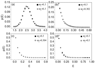
Figure 5: Distributions of energy for oscillator 1 (black squares) and oscillator 2 (gray circles) for the four cases displayed in Fig. 4. The distribution is Gaussian in the resonant case (panel (a), centered in $\bar{E}=2.5$), and Boltzmann-like in all off-resonant cases: $p_{B}(E)=\exp{(-E/\bar{E}_{i})}/\bar{E}_{i}$ with $\bar{E}_{1}\approx 0.072$ and $\bar{E}_{2}\approx 0.073$ (panel(b)); $\bar{E}_{1}\approx 0.072$ and $\bar{E}_{2}\approx 0.073$ (panel(c)); and $\bar{E}_{1}\approx 0.075$ and $\bar{E}_{2}\approx 0.069$ (panel(d)).

Non-Resonant case: Panels (b) to (d) in Fig. 4 show the energy of the oscillators for frequencies moving away from the resonance. It is still possible to see a flow of energy from one oscillator to the other, although this becomes less evident as the frequencies become more separated. Also visible is the increase in the dissipated energy. Fig. 4 also shows how sensitive is the dynamical behavior of the system with respect to variations in the frequency of the oscillators. In the quasi-resonant cases (see panels (b) and (c)), where $\omega_{1}/\omega_{2}\approx 1$, the relaxation time is significantly greater than in the other cases, allowing energy exchange between the oscillators for a very long time. However, if the ratio $\omega_{1}/\omega_{2}$ deviates more considerably from unity (panel (d)), the “opacity” of the chaotic medium increases, culminating in almost independent oscillators that quickly lose all their energy to the environment. The energy distributions corresponding to the cases of Fig. 4 are depicted in Fig. 5, and show that the finite environment does act as a thermal bath for the two oscillators, both of which have the same temperature. Moreover, the equipartition theorem holds true for all three off-resonant cases at long times, which means that the relation $\bar{E}_{1}\approx\bar{E}_{2}\approx\tfrac{2}{3}\bar{E}_{QS}$ is valid. This reinforces the ability of the finite chaotic environment to promote dissipation and thermalization Marchiori and de Aguiar (2011). Nevertheless, the resonance condition permits an efficient flow of energy between the harmonic modes. The aim of next section is to explain the special resonant case, and show that in this case the equipartition is still valid.

VI Linear response theory

The oscillators obey the dynamics given in the equations

$$\ddot{q}_{i}+\omega_{i}^{2}q_{i}=-\frac{\lambda_{N}}{m}\sum_{n=1}^{N}x_{n}\equiv-\frac{\lambda_{N}}{m}\,X(t).$$ (17)

As the dynamics of the variables $x_{n}$ are chaotic and the interaction among the QS’s is of second order in the coupling, each $x_{n}$ is approximately independent and we may replace $X(t)$ by its average $\langle X(t)\rangle$. Applying then linear response theory (LRT) Kubo et al. (1985), we get

$$\ddot{q}_{i}+\omega_{i}^{2}q_{i}\approx\frac{\lambda^{2}_{N}}{m}\int^{t}_{0}ds\,\phi_{XX}(t-s)(q_{1}(s)+q_{2}(s))\,,$$ (18)

where the response function $\phi_{XX}$ is given in Ref. Marchiori and de Aguiar (2011) by

$$\phi_{XX}(t-s)=\frac{5\mu N}{4}\frac{d}{ds}\delta(t-s)+\frac{\mu N(t-s)}{4}\frac{d^{2}}{dtds}\delta(t-s)\,,$$ (19)

where $\mu$ is a parameter that depends on the average energy of the environment. After computing the integral we have

$$\ddot{q}_{1}+\gamma\dot{q}_{1}+\omega_{1}^{2}q_{1} = -\gamma\dot{q}_{2},$$ (20)

$$\ddot{q}_{2}+\gamma\dot{q}_{2}+\omega_{2}^{2}q_{2} = -\gamma\dot{q}_{1}$$ (21)

with $\gamma=\frac{3\lambda^{2}\mu}{8m}$. These equations cannot be diagonalized unless $\omega_{1}=\omega_{2}$. In this case, we can define the new variables

$$Q_{\pm}=\frac{q_{1}\pm q_{2}}{\sqrt{2}},$$ (22)

associated with center-of-mass and relative coordinates of the oscillators, and rewrite (20) and (21) as

$$\ddot{Q}_{+}+2\gamma\dot{Q}_{+}+\omega^{2}Q_{+} = 0,$$ (23)

$$\ddot{Q}_{-}+\omega^{2}Q_{-} = 0.$$ (24)

The $Q_{-}$ is then completely decoupled from the environment, and will be called the conservative mode, whose initial energy is $E_{1}(0)/2$ for the present initial conditions. Analogously, $Q_{+}$ will be termed dissipative mode. LRT predicts $\gamma\ll\omega$; therefore $Q_{+}$ dissipates energy according to $E_{+}(t)\approx E_{+}(0)\exp\left({-2\gamma\,t}\right)$, where $E_{+}(0)$ is also $E_{1}(0)/2$. Note that Eq. (24) is exact, as can be seen by replacing (22) into (17).

The harmonic oscillators energies obtained from Eqs. (20) and (21) are compared in Fig. 4 with numerical simulations of the Hamiltonian (1). As seen from the figure, the qualitative agreement is excellent for both resonant (panel (a)) and non-resonant (panel (d)) cases.

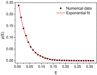
Figure 6: (Color online) Distribution of energy for the dissipative $Q_{+}$-mode for $N=100$. The fit is $p_{B}(E)=\exp{(-E/\bar{E}_{+})}/\bar{E}_{+}$ with $\bar{E}_{+}=0.037$.

In order to correctly apply the equipartition theorem in the resonant case we have to consider only the energy in $Q_{+}$. Taking the expression for the total initial energy, $E_{T}=E_{1}/2+NE_{QS}$, we find that the expected value of the energy of the dissipative mode in equilibrium is $\bar{E}_{+}\approx 0.039$. This is confirmed in Fig. 6, which shows the energy distribution of $Q_{+}$. Therefore, the violation of equipartition was only apparent, caused by the emergence of a conservative mode that prevented the complete dissipation of the energy in the harmonic oscillators.

VII Conclusions

We have studied the dynamical behavior of two harmonic oscillators independently coupled to a chaotic environment with $2N$ degrees of freedom. We focused our analysis on two points: the interactions between the oscillators mediated by the chaotic environment and the equilibrium properties of the system. We found that the oscillators can exchange energy through the environment when in almost perfect resonance. Deviations from this condition quickly changes this behavior and makes the oscillators less sensitive to the presence of each other. When in perfect resonance, the oscillators are able to keep part of their initial energy in an apparent violation of the equipartion theorem. This, however, turns out to be exactly the fraction of the energy stored in the oscillators relative motion, which is not coupled to the environment. This holds both for $N=1$ via ensemble averages or for $N=100$ for a single realization of the dynamics and is also true within the approximation of the linear response theory, which works well for the resonant and non-resonant cases.

The equilibrium properties of the system, on the other hand, depend critically on the number of degrees of freedom of the environment. In order to quantify the equilibrium we considered two measures of temperature: $\tau_{E}$, obtained from the equipartition theorem, and $\tau_{S}$, obtained via the usual definition of entropy. These temperatures were also compared with the energy distribution of each subsystem, whenever these converged to a Boltzmann-like exponential. For $N=100$ the oscillator’s energy distributions indeed always converged to the exponential decay $\exp{(-E/\tau_{B})}$ with $\tau_{B}\approx\tau_{E}$ for all subsystems, except in the resonant cases. This characterizes the thermal equilibrium and corroborates earlier results that a not too small chaotic environment does play the role of a thermal bath Marchiori and de Aguiar (2011). This conclusion also holds in the resonant case if the energy of the conservative mode is properly subtracted.

The case $N=1$, on the other hand, showed a very rich behavior. Equilibration takes very long times for the present choice of parameters and the energy distribution of the oscillators display, in some cases, exponential curves. Curiously, for the particular values of $\omega_{1}$ and $\omega_{2}$ used, the exponent agreed reasonably with energy equipartition, but not with $\tau_{S}$. Moreover, the distribution of the momentum did often displayed the expected Gaussian distribution, even if the corresponding energy distribution was not exponential. These unexpected results show that the $N=1$ environment does not simulate the action of a thermal bath even if averaged over an ensemble of trajectories, and display a more complicated type of approach to equilibrium that is worth a deeper investigation.

We have also examined the ergodicity of the system. Because $\lambda$ is small, it could be expected that the total system would not be ergodic. This, however, is not the case. For $\lambda=0$, the environment is ergodic for $N=1$ but it is not ergodic for $N=100$, since the quartic systems are totally independent from each other. As the coupling is turned on, the total system becomes ergodic for $N=100$ (and is able to show the correct equipartition of energy), whereas, for $N=1$, it does not. This was verified by numerical results not shown in which time and ensemble averages were compared for various conditions. As expected, we found that temperature could be defined whenever ergodicity was satisfied, although ergodicity itself depends non-trivially on the parameters of the system and on the number of degrees of freedom.

Finally, we note that the emergence of the conservative mode $Q_{-}$ depends on the symmetry of the coupling as given in Eq. (4) and on the resonance condition $\omega_{1}=\omega_{2}$. The conservative mode is absent if $\omega_{1}\neq\omega_{2}$ or if each oscillator is coupled to a different mode of the quartic system, such as in $H_{I}=\sum_{n}(q_{1}x_{n}+q_{2}y_{n})$. In LRT this leads to decoupled equations for $Q_{+}$ and $Q_{-}$, each equation identical to Eq. (23).

- (1) A. O. Caldeira and A. J. Leggett, Ann. Phys. 149, 374 (1983); erratum, 153, 445 (1984).
- (2) A. O. Caldeira and A. J. Leggett, Physica A 121, 587 (1983); erratum, A 130, 374 (1985).
- (3) M. P. A. Fisher and W. Zwerger, Phys. Rev. B 32, 6190 (1985).
- (4) U. Weiss, Quantum dissipative systems (World Scientific, Singapore, 1993).
- (5) P. Hedegard and A. O. Caldeira, Phys. Scr. 35, 609 (1987).
- (6) N. V. Prokof’ev and P. C. E. Stamp, Rep. Prog. Phys. 63, 669 (2000).
- Wilkinson (1990) M. Wilkinson, J. Phys. A: Math. Gen. 23, 3603 (1990).
- (8) M. V. Berry and J. M. Robbins, Proc. R. Soc. London A 442, 659 (1993).
- (9) T. O. de Carvalho and M. A. M. de Aguiar, Phys. Rev. Lett. 76, 2690 (1996).
- Cohen (1999) D. Cohen, Phys. Rev. Lett. 82, 4951 (1999).
- (11) D. Cohen and T. Kottos, Phys. Rev. E 69, 055201 (2004).
- Marchiori and de Aguiar (2011) M. A. Marchiori and M. A. M. de Aguiar, Phys. Rev. E 83, 061112 (2011).
- Bonanca and de Aguiar (2006) M. V. S. Bonança and M. A. M. de Aguiar, Physica A 365, 333 (2006).
- (14) O. S. Duarte and A. O. Caldeira, Phys. Rev. Lett. 97, 250601 (2006).
- (15) O. S. Duarte and A. O. Caldeira, Phys. Rev. A 80, 032110 (2009).
- (16) D. M. Valente and A. O. Caldeira, Phys. Rev. A 81, 012117 (2010).
- (17) W.-H. Steeb, J. A. Louw, and C. M. Villet, Phys. Rev. A 34, 3489 (1986); M. P. Joy and M. Sabir, Pramana J. Phys. 40, 17 (1993).
- (18) R. C. Tolman, Phys. Rev. 11, 261 (1918).
- (19) V. L. Berdichevsky and M. V. Alberti, Phys. Rev. A 44, 858 (1991).
- (20) H. H. Rugh, Phys. Rev. Lett. 78, 772 (1997); H. H. Rugh, J. Phys. A: Math. Gen. 31, 7761 (1998).
- (21) O. G. Jepps, G. Ayton, and D. J. Evans, Phys. Rev. E 62, 4757 (2000); G. Rickayzen and J. G. Powles, J. Chem. Phys. 114, 4333 (2001); J. G. Powles, G. Rickayzen, and D. M. Heyes, Molec. Phys. 103, 1361 (2005).
- (22) V. M. Bannur, Phys. Rev. E 58, 407 (1998); B. D. Butler, G. Ayton, O. G. Jepps, and D. J. Evans, J. Chem. Phys. 109, 6519 (1998); G. P. Morriss and L. Rondoni, Phys. Rev. E 59, R5 (1999); V. M. Bannur, Phys. Rev. C 72, 024904 (2005).
- (23) G. Birkhoff and G.-C. Rota, Ordinary differential equations (Wiley, New York, 1989).
- Kubo et al. (1985) R. Kubo, M. Toda, and N. Hashitsume, Statistical Physics II: Nonequilibrium Statistical Mechanics (Springer-Verlag, Berlin, 1985).