We present some simple pen and paper examples of trapped surfaces in order to help visualising this key concept of the theory of gravitational collapse. We collect these examples from time-symmetric initial data, 2+1 dimensions, collapsing null shells, and the Vaidya solution.

1. Introduction

Provided an appropriate positivity property holds the existence of a closed trapped surface has dramatic consequences for the future evolution of spacetime. In numerical relativity trapped surfaces provide—assuming that a cosmic censor is active—the practical means by which black holes are recognized, and indeed effective algorithms to spot trapped surfaces in a given initial data set have been developed [1]. There are also theorems in mathematical relativity that tell us much about the existence of marginally trapped surfaces [2, 3, 4, 5, 6, 7, 8], their “evolution” into marginally trapped tubes foliated by such surfaces [9, 10], and their formation from initial data sets that are free of them [11]. A possible application is to quasi-local definitions of black holes [12, 13, 14, 15]: the numerical algorithms are not called “horizon finders” for nothing. Other chapters in this book provide the details. The modest aim here is a supplementary one: we will collect some illustrative examples of trapped surfaces that one can obtain with pen and paper only.

After some preliminaries in section 2, we discuss time-symmetric initial data of the Einstein equations in section 3. Early studies initiated by Wheeler and pursued by Brill and Lindquist [16] and many others [17, 18, 19, 20] led to the construction of initial data containing an arbitrary number of Einstein-Rosen bridges to new asymptotic regions, and to interesting observations on the minimal surfaces that appear there. Although the term was not used—because the notion of trapped surfaces had not yet been introduced—these surfaces are in fact marginally trapped in the resulting spacetime. In section 4 we restrict ourselves to a 2+1 dimensional toy model of gravity (with a negative cosmological constant) [21, 22, 23, 24], where a complete description of all marginally trapped “surfaces” in spacetime can be had [25]. In this toy model we will also see how the trapped surfaces “jump” when we throw lumps of matter into a black hole [26], and—by increasing the dimension again—what a dynamical horizon can look like in the vacuum case [27].

In 3+1 dimensions trapped surfaces can be produced in a controlled manner by sending convex shells of incoherent radiation into flat spacetime. This idea was proposed by Penrose [28] as a way to test cosmic censorship; it has been much studied [29, 30, 31] and will be discussed in section 5. Following, say, a marginally trapped tube into the future is a more difficult matter, but in section 6 we say more about the spherically symmetric Vaidya solution [32, 33, 34, 35, 36, 37]. This is possible because spherical symmetry prevents gravitational radiation from appearing behind the shell.

For natural reasons there will be a certain emphasis on trapped surfaces I have encountered myself—with apologies to authors who feel, perhaps rightly so, that their own examples are more interesting.

2. Preliminaries

We are interested in the way a submanifold is embedded into some larger space, so for this purpose we decompose the tangent space at a point of the submanifold into a tangential and a normal part. If $X$ and $Y$ are vector fields belonging to the former the Weingarten or shape tensor $K$ will produce a vector belonging to the latter according to its definition

$$K(X,Y)=-(\nabla_{X}Y)^{\perp}\ .$$ (1)

Here $\nabla_{X}$ is the usual covariant derivative along the tangential direction $X$. For an actual computation we may assume that the submanifold is given in parametric form, $x^{a}=x^{a}(u)$, and we find that the Weingarten tensor contracted into a normal vector $k^{a}$ is

$$K_{ij}(k)=-k_{a}\frac{\partial^{2}x^{a}}{\partial u^{i}\partial u^{j}}-k_{a}\Gamma_{bc}^{\ \ a}\frac{\partial x^{b}}{\partial u^{i}}\frac{\partial x^{c}}{\partial u^{j}}\ .$$ (2)

In the examples below such a calculation is typically either straightforward but tedious, or hideously complicated. The details will be relegated to the list of references.

If the submanifold has codimension 1 the normal vector is unique, and the Weingarten tensor is referred to as the second fundamental form—but trapped surfaces have codimension 2 by definition. In any case the first fundamental form $\gamma_{ij}$ is the metric induced on the submanifold, and the mean curvature vector is defined by

$$H^{a}=\gamma^{ij}K_{ij}^{a}\ .$$ (3)

In Riemannian spaces it can be shown that the surface is minimal—meaning that its area always increases if the surface is subject to variations of sufficiently small compact support—if and only if its mean curvature vector vanishes. For hypersurfaces the mean curvature vector contracted into the unique normal vector is called the mean curvature, denoted $K$.

As part of its definition a trapped surface is a spacelike surface of codimension 2, in a Lorentzian spacetime. It follows that any normal vector can be expressed as a linear combination of two future directed null vectors, normalised by

$$k_{+}\cdot k_{-}=-2\ .$$ (4)

As the notation suggests, one of these vectors ($k_{+}$) will be directed “outwards” and the other “inwards”. The set of all such vectors will give rise to one outgoing and one ingoing null congruence, and the surface is said to be trapped if the cross sections of both congruences decrease in area as they leave the surface. Whether this is so can be read off from the mean curvature vector, which is

$$H^{a}=-\theta_{+}k_{-}^{a}-\theta_{-}k^{a}_{+}\ .$$ (5)

The surface is trapped if both the null expansions $\theta_{\pm}$ are negative, meaning that the mean curvature vector is timelike and future directed. The surface is marginally trapped if the outer expansion $\theta_{+}=0$ and the inner expansion $\theta_{-}\leq 0$.

Actually, in the algorithms that look for marginally trapped surfaces, only the outwards expansion is controlled [1]. Hence they produce marginally outer trapped surfaces, where the meaning of “outer” is provided by some spacelike slice in which the surface is embedded. It turns out that the main body of mathematical relativity theorems concerns marginally outer trapped surfaces, and that such surfaces suffice to prove singularity theorems [10]. But we will concentrate on genuinely trapped and marginally trapped surfaces (with $\theta_{-}\leq 0$) here, partly because the marginally trapped tubes swept out by a sequence of such surfaces have particularly interesting properties [13, 14].

In 2+1 dimensional Minkowski space, which is helpful for visualisation, a codimension 2 submanifold is simply a curve. Let it be spacelike. It is future trapped if its Frenet normal vector is timelike and future pointing, and untrapped if the normal vector is spacelike. A marginally outer trapped curve is a curve in some null plane, and its inner expansion is negative if and only if that curve is concave. It will be observed that only the untrapped curves can be closed. From now on, when we talk of a trapped surface we often assume that it is closed—since otherwise its existence has no particular consequences. In this sense there are no closed trapped surfaces in Minkowski space. If space has the topology of a cylinder we find that there are closed marginally outer trapped curves in suitable null planes, but still none with $\theta_{-}<0$ everywhere.

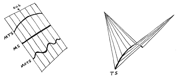
Figure 1: A null plane containing marginally trapped, minimal, and marginally outer trapped curves. Note that any spacelike plane crossing the null plane will contain a curve of the latter type. A locally trapped curve (a piece of a hyperbola bending down in time) is on the right.

The Riemannian cousins of marginally trapped surfaces are the minimal surfaces, and many beautiful examples have been published. Based on Plateau’s experiments with soap films spanned by thin wires [38], it was conjectured that one can find a minimal surface with any given one dimensional boundary. This was proved with mathematical precision some eighty years later [39]. But the boundary is essential—closed minimal surfaces do not exist in Euclidean space. A way to see this is to observe that the equation obeyed by the functions $x^{a}(u)$ when the first variation of the area functional vanishes is the Laplace equation.

Thus in flat space a minimal surface needs a boundary, but we can do better if we are inside the 3-sphere. Indeed the solution of the Plateau problem, together with a scheme using reflections, can then be used to produce closed minimal surfaces of any genus [40]. For genus 0 and 1 it is easy to see what these minimal surfaces are. The equator of the 3-sphere is a minimal 2-sphere, and the maximal torus that appears in the Hopf fibration is a minimal 2-torus. Like the geodesics—the great circles on the sphere—they are in a sense “maximal” rather than minimal, because there exists a global deformation that decreases their area. The technical term for such minimal surfaces is “unstable”.

Although they are not based on any variational principle, the notion of stability can be generalised so as to apply to marginally outer trapped surfaces [3, 10]. Moreover a Plateau problem can be formulated and solved for them [6].

A totally geodesic submanifold is a submanifold such that the entire Weingarten tensor vanishes. This means that a geodesic starting out tangential to the submanifold will stay in the surface, where it defines a geodesic with respect to the intrinsic metric as well. Unless their dimension is equal to one—a geodesic—such submanifolds typically do not exist, but if the embedding space has a large amount of symmetry they may. In particular, the fixed point set of an isometry is always totally geodesic. (This is easy to see. Consider a vector tangent to the surface at some point. This defines a unique geodesic in the embedding space. If this geodesic were able to move out of the surface a part of it would be moved by the isometry, while its starting point and its initial tangent vector would not be. This contradicts the uniqueness of the geodesic.) In general relativity a totally geodesic spacelike hypersurface occurs whenever time-symmetric initial data exist, and we can then rely on the useful fact that a minimal surface in such an initial data hypersurface is a marginally trapped surface in the resulting spacetime.

3. Time-symmetric initial data

The initial data for Einstein’s equations are given by the first and second fundamental forms (two symmetric tensor fields on some space, one of them being its metric), subject to suitable constraints. If we take the second fundamental form to vanish—so that we will have a totally geodesic hypersurface in the spacetime to be constructed—the constraint on the first fundamental form take the simple form

$$R^{(3)}=0\ .$$ (6)

Its curvature scalar vanishes. This assumes vacuum, with vanishing cosmological constant. We may simplify matters further by assuming that the intrinsic metric takes the form

$$ds^{2}=\omega^{4}(dx^{2}+dy^{2}+dz^{2})\ .$$ (7)

This was referred to as “geometrostatics” in the early references [16, 17]. The reason for the unusual exponent on the conformal factor is that eq. (6) now takes the form

$$\triangle\omega=0\ ,$$ (8)

where $\triangle$ is the flat space Laplacian. From electrostatics we know how to solve this. A suitable solution is

$$\omega=1+\sum_{i=1}^{N}\frac{e_{i}}{r_{i}}\ ,$$ (9)

where the source points can be placed at $N$ arbitrary positions, and $r_{i}$ is the Euclidean distance to the $i$th source point.

If there is only one source point, placed at the origin, and if we use spherical polar coordinates $(r,\theta,\phi)$, this is the $t=0$ slice of the Schwarzschild solution in isotropic coordinates. Its mass $M=2e$. This geometry admits a discrete isometry under

$$r\rightarrow r^{\prime}=\frac{e^{2}}{r}\ .$$ (10)

From this we learn two things. First, that the source points in the solution do not represent singular points in the geometry, they represent the spatial infinities in $N$ (out of $N+1$) asymptotic regions. Second, when $N=1$ the sphere at $r=e=M/2$ is a fixed point set of an isometry, hence it is totally geodesic and by implication a minimal surface. When the geometry evolves it becomes the bifurcation sphere on the event horizon.

The case when there are more than two asymptotic regions (when $N>1$) is made intuitively clear in the illustrations provided by Brill and Lindquist [16]. See Fig. 2. There will be $N$ throats leading from the original asymptotically flat sheet to an additional $N$ such sheets. In each throat we will find a minimal 2-sphere, but it will no longer be a round sphere—rather it will be distorted by its interaction with the others. If the throats are well separated this is the end of the story, but if two throats come sufficiently close together an additional minimal sphere will appear and surround the two minimal spheres in the throats.

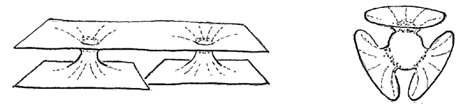
Figure 2: Brill-Lindquist initial data: When the throats are far apart there are only two minimal surfaces. In the symmetric case shown to the right there are obviously three.

To see how this works, let us choose $N=2$ and $e_{1}=e_{2}$. The conformal factor is

$$\omega+\frac{e}{r_{1}}+\frac{e}{r_{2}}=1+\frac{e}{\sqrt{\rho^{2}+z^{2}}}+\frac{e}{\sqrt{\rho^{2}+(z-a)^{2}}}\ ,$$ (11)

where $a$ is the Euclidean distance between the two source points, and cylindrical coordinates were introduced in the second step. It is not difficult to read off the ADM masses in the three external regions, by studying how the metric falls off at infinity (using the coordinate $r^{\prime}_{1}=e_{1}^{2}/r_{1}$ as a coordinate in the first region, say). One finds [16]

$$M_{1}=M_{2}=2e\left(1+\frac{e}{a}\right)\ ,\hskip 17.07164ptM_{3}=4e\ .$$ (12)

It is clear that if $a>>e$ the two throats will not affect each other much, and there will be only two minimal spheres. But if $a=e$ all three masses will be equal, and by symmetry there will be three throats, and three minimal spheres. Interestingly the area of the outermost minimal sphere—outermost from the point of view of the third external region—is smaller than the sum of the areas of the two minimal spheres it is surrounding. This will be so whenever the distance $a$ is small enough. There must exist a critical value $a_{\rm cr}$ when the third minimal sphere first appears. To calculate this we assume that any minimal surface is axisymmetric and given by $\rho=\rho(\sigma)$, $z=z(\sigma)$, $\phi=\varphi$. The minimal surface equation is then obtained by extremising the area functional

$$A=\int\sqrt{\det\gamma}d\sigma d\varphi=2\pi\int_{\sigma_{0}}^{\sigma_{1}}\rho\omega^{4}\sqrt{\dot{\rho}^{2}+\dot{z}^{2}}d\sigma\ .$$ (13)

We must find solutions corresponding to closed surfaces. Unfortunately—because the stated purpose of this review is to give pen and paper examples—numerical methods must be used to do this. Moreover the numerical calculation is non-trivial, as is clear from the fact that the first attempts to do it did not give quite the correct answer. The conclusion eventually turned out to be that the critical Euclidean distance is $a_{\rm cr}\approx 1.53e$ [19], and in fact a pair of minimal surfaces are created when we go below this value [20].

Do take note of the fact that the surrounding minimal sphere is there for a reason. We assume that cosmic censorship holds, and that we have found the area $|S|$ of a—not necessarily connected—trapped surface in our initial data. Then there must be an event horizon intersecting the initial hypersurface, and since it lies outside the trapped surface we expect its area to be larger than $|S|$. In the future we expect the system to settle down into a Kerr black hole, and since the area of the event horizon can only grow the area of the final event horizon is also larger than $|S|$. Some of the initial mass $M$ will be radiated away, so the area of the final event horizon—which is never larger than the area of a Schwarzschild horizon of the same final mass—will be no larger than $16\pi M^{2}$. Tracing through this string of inequalities we find that

$$16\pi M\geq\sqrt{16\pi|S|}\ .$$ (14)

The mass $M$ and the area $|S|$ are determined by the initial data. This interesting strengthening of the positive mass theorem is known as the Penrose inequality, and should be a necessary (but not sufficient!) condition for cosmic censorship to hold [28]. But as the two throats in the Brill-Lindquist initial data are moved closer together, the sum of their areas grow [16]. In fact their sum can exceed the bound set by the Penrose inequality. What saves the day is precisely the new minimal surface that appears out of the blue to surround the two, and now counts as outermost [18].

A possible loop hole in the above argument—quite apart from a possible failure of cosmic censorship—appears in its first step, since it is not clear that a surface that surrounds another must have a larger area. However, in the case of time-symmetric data the marginally trapped surfaces are minimal and the reasoning does not need any amendment, provided the trapped surface is taken to be the (not necessarily connected) outermost marginally trapped surface. One can construct simple examples in Oppenheimer-Snyder dust collapse where more care is needed [41, 42].

4. The 2 + 1 dimensional toy model

To bring the multi-black hole problem within the range of pen and paper methods Brill [23], and Steif [24], eventually turned to 2 + 1 dimensions where a trapped “surface” is a closed spacelike curve with a future pointing timelike Frenet normal vector. There are considerable simplifications because there is no Weyl tensor and no shear in the Raychaudhuri equation for a null congruence: in 2+1 dimensions

$$\dot{\theta}=-\theta^{2}-R_{ab}t^{a}t^{b}\ .$$ (15)

If we impose Einstein’s vacuum equation $R_{ab}=\lambda g_{ab}$ the second term vanishes, $\dot{\theta}=-\theta^{2}$, and hence

$$\theta(0)=0\hskip 14.22636pt\Leftrightarrow\hskip 14.22636pt\theta(\tau)=0\ .$$ (16)

This has the consequence that a marginally trapped surface must lie on a lightlike plane, or—to use a terminology that is more accurate in the de Sitter and anti-de Sitter cases—on a lightcone with its vertex on . In turn this means that we can easily get a complete overview of all marginally (outer) trapped curves in a spacetime of this type. Still, even though the vacuum equations imply that spacetime has constant curvature, the model is not completely trivial.

There are no closed trapped curves in Minkowski space, but they do exist in a suitable region of Misner space, which is Minkowski space with points related by some discrete Lorentz boost identified [2]. Since the boost has a line of fixed points there is a kind of singularity to the future of such a trapped curve, as well as a breakdown of the causal structure in the form of closed timelike curves. Misner space does not have a black hole, since it has no sensible notion of future , but the same construction carried out in anti-de Sitter space has. It gives rise to the BTZ black hole [21]. To see how this works consider the metric of 2 + 1 dimensional anti-de Sitter space,

$$ds^{2}=-\left(\frac{1+\rho^{2}}{1-\rho^{2}}\right)^{2}dt^{2}+\frac{4}{(1-\rho^{2})^{2}}(d\rho^{2}+\rho^{2}d\phi^{2})\ .$$ (17)

At $t=0$ we have a time-symmetric initial data slice which in these coordinates appears in the guise of the Poincaré disk, a space of constant negative curvature. The group of isometries preserving this slice is isomorphic to the subgroup of Möbius transformations that preserve its conformal boundary (in these coordinates the unit circle). Among them are the hyperbolic Möbius transformations, that have two fixed points on the boundary of the disk and a special flow line which is the unique geodesic connecting the fixed points—we recall that the geodesics on the Poincaré disk are arcs of circles or straight lines meeting the boundary at right angles.

Now pick such a Möbius transformation, obtainable by exponentiating an infinitesimal transformation. We identify all the points one can connect with it. The result is a space of constant curvature and cylindrical topology, having exactly one closed geodesic—a minimal “surface”—corresponding to the unique geodesic flow line. These are the initial data of the BTZ black hole (and occurs as panel a in Fig. 4). Since anti-de Sitter space is not globally hyperbolic these data do not in fact determine the future evolution, but we can define the spacetime as the quotient of anti-de Sitter space with the discrete isometry group generated by the group element we used to construct our initial data. This spacetime is the BTZ black hole [21]. It has a singular future (since the isometry will have fixed points to the future, and to the past, of the initial data slice), and it will be asymptotically anti-de Sitter in the sense that the first order structure of the quotiented conformal boundary is conformally isomorphic to the 1+1 Einstein universe, the  of anti-de Sitter space [22]. The event horizon is the boundary of the past of , as usual.

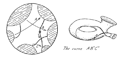
Figure 3: An initial data surface for a black hole spacetime with two asymptotic regions. The white part is a fundamental region. The group $\Gamma$ is generated by the group elements $A,B,C$, and a closed curve associated to the group element $AB^{-1}C^{-1}$ is shown. Reproduced with permission [43].

This idea can be generalised. Given a pair of geodesics on the Poincaré disk at $t=0$ there is a unique hyperbolic Möbius transformation taking one to the other. If we choose several such pairs of geodesics—in Fig. 3 we choose three pairs—we obtain several group elements. If we make sure that the geodesics do not intersect these group elements generate a free group $\Gamma$, and we define our spacetime as the quotient of anti-de Sitter space by $\Gamma$. Its initial data surface at $t=0$ is guaranteed to be a smooth surface of constant negative curvature and one or several asymptotic regions. We can now search for closed geodesics—marginally trapped surfaces—on this initial data surface.

But this is not a hard task. Take any closed curve in the quotient space. It can be associated to a particular element in the discrete group $\Gamma$, as shown by example in Fig. 3. This group element is in itself a hyperbolic Möbius transformation, and is therefore associated with a unique geodesic flowline. The latter will become a closed geodesic in the quotient space. In this way we find one closed marginally trapped curve for every topologically distinct class of closed curves. From a spacetime point of view, and from our discussion of the Raychaudhuri equation, we know that a marginally trapped curve must lie on a lightcone with its vertex on . This vertex can be found by analysing the action of $\Gamma$ on , but since this pleasant task has been described elsewhere we do not go into this here [25].

I should add that the restriction to time symmetric spacetimes can be lifted, at the expense of rather more work [43].

To get a more lively picture we can try to add some matter to the model. So as to not compromise its basic simplicity this is often done in the form of “point particles”, conical singularities with their vertices along timelike or null geodesics [44]. There will be a non-trivial holonomy associated to any spacelike curve surrounding the singular geodesic, and from this one can read off the “mass” of the resulting spacetime. Now suppose we start with a single BTZ black hole, choose a radial null geodesic leaving  and heading for the event horizon, choose a suitable wedge with that geodesic as its edge, and identify the two boundaries of the wedge using an element of the isometry group. This then describes a lump of matter falling into a black hole, and the question arises how it will affect the black hole when it hits [26].

In any dimension one expects the outermost marginally trapped surface to “jump” outwards when a lump of matter hits it. It will be a somewhat non-local jump since it takes place also on that side of the black hole which is not yet in causal contact with the infalling matter. What happens there is that some locally trapped surface is “suddenly” a part of a closed trapped surface because of the way the lump of matter curves space elsewhere—while it would have been part of an open surface if no matter had been falling in. But this is not a spherically symmetric situation, and gravitational radiation will prevent any pen and paper calculation from being made—unless we are in 2+1 dimensions, where gravitational radiation does not happen.

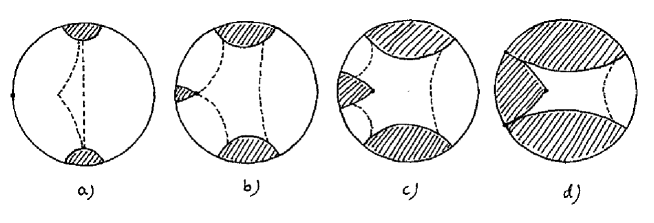
Figure 4: a) The particle comes in from infinity just as a marginally trapped curve is formed in the centre. The event horizon has a kink and does not contain any marginally trapped curves. b) The particle meets the event horizon. c) The event horizon is now smooth and marginally trapped. d) The identification surfaces meet in a singular point at infinity. Reproduced with permission [26].

Concretely, let a massless particle enter a BTZ black hole spacetime at $t=0$ (panel a in Fig. 4). We follow the time development by slicing covering space with a sequence of Poincaré disks at increasing values of $t$. The particle moves inwards trailing its wedge behind it. Meanwhile the geodesic arcs that bound the fundamental region of the BTZ black hole are moving closer to each other. Eventually they meet the boundary of the wedge; the result is a fixed point on  that corresponds to a singular point in the quotient space (which will then continue inwards along a spacelike geodesic). The backwards light cone from that singular point is the event horizon of the resulting spacetime.

Following the event horizon backwards in time we observe that it is a smooth surface foliated by closed marginally trapped curves only as long as it passes through the wedge behind the particle (down to panel b in Fig. 4). At earlier times the event horizon has a kink, and does not contain any smooth and closed spacelike curves. Yet there is a closed marginally trapped curve at $t=0$, namely the one that would have evolved into the event horizon of the BTZ black hole, had there been no massless particle to complicate matters. This will evolve into an isolated horizon which is destroyed by its encounter with the particle (in panel c, although only the horizon bordering the second asymptotic region is shown in the figure). A spacetime picture of all this is given in Fig. 5.

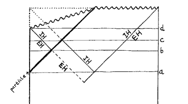
Figure 5: A conformal diagram of a massless particle falling into a BTZ black hole. Four spatial slices corresponding to the panels in Fig 4 are given, and we also see how the isolated horizon (IH) “jumps”.

As a final remark, let us go to 3+1 dimensions by means of the obvious amendment of the metric (17), i.e. by adding an extra angular coordinate $\theta$. At $t=0$ we now have a Poincaré ball, and there are isometries mapping totally geodesic surfaces—spherical caps meeting the boundary at right angles—to each other. Take the quotient of 3 + 1 dimensional anti-de Sitter space with such an isometry. The result is a genuine black hole spacetime, but a curious one since its event horizon is not a Killing horizon. It grows. One can now look for marginally trapped surfaces in a slicing that respects the symmetries of the quotient space, and one finds that they foliate a spacelike dynamical horizon situated well inside the event horizon [27]. The conformal boundary is connected, and has the topology of a torus times the real line. This pathological feature apart it is an interesting example.

5. Collapsing null shells

A rich supply of interesting trapped surfaces can be had by sending a thin shell of incoherent radiation (also known as null dust) into Minkowski space. The surfaces will arise as cross sections of the null shell. We want the interior of the shell to remain flat, meaning that the shell cannot have caustics to the past of the surface. To ensure this we insist that its cross section with some spacelike hyperplane is convex. To the future the generators of the shell cross, and a spacetime singularity results. About the outside of the shell we know very little—unless the shell and the mass distribution are spherically symmetric there will be gravitational radiation there. If a cosmic censor is active a black hole will develop, and eventually settle down to the Kerr solution. Again we have the Penrose inequality (14); in fact this was the setting in which the inequality was first proposed [28]. What is remarkable about the shell construction is that both $M$ and $|S|$ can be evaluated without knowledge of the exterior of the shell. They result from calculations in flat space.

The energy-momentum tensor of the shell is

$$T^{ab}=8\pi\mu k_{-}^{a}k_{-}^{b}\delta\ ,$$ (18)

where $\mu$ is an arbitrary function on a cross section and the delta function is defined with respect to the volume form induced by the ingoing null normal $k_{-}^{a}$. We now choose the cross section we want by intersecting the shell with an outgoing null congruence having outer null expansion $\theta_{+}^{\rm int}$. This null expansion will jump at the shell. From the Raychaudhuri equation we obtain

$$\theta_{+}^{\rm ext}=\theta_{+}^{\rm int}-16\pi\mu\ .$$ (19)

Since the mass distribution $\mu$ is at our disposal we can turn any cross section into a marginally trapped surface in this way. Moreover we can search for trapped surfaces on the shell—in particular for the outermost marginally trapped surface—in an efficient way.

As an example of the kind of insights one can get from this model, consider the case when the shell admits an ellipsoidal cross section. Using a foliation of Minkowski space with the usual $t=$ constant hypersurfaces one then finds that the caustic appears first at the ends, and so does any trapped surface sitting on the shell. The result is that there are no trapped surfaces on any $t=$ cross section before the value of $t$ for which the singularites first appears [31]. This provides some food for thought, given that the numerical algorithms look for marginally trapped surfaces in given spacelike hypersurfaces [1]. (Even in the Schwarzschild solution it is known that there exists a foliation with spacelike hypersurfaces which reaches all the way to the singularity even though its leaves do not contain any trapped surfaces [45]. But that foliation was chosen specifically to make this true, while the foliation used for the collapsing shell is perfectly natural.)

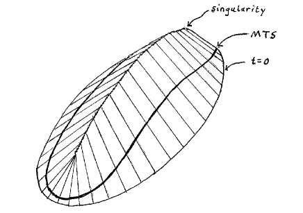
Figure 6: A collapsing null shell considered by Pelath, Tod and Wald [31]: It has an ellisoidal cross section at $t=0$. Both the singularity and the first marginally trapped surface “bend” in time in such a way that the singularity appears at an earlier value of $t$ than does the last piece of the marginally trapped surface.

The proof of the Penrose inequality remains partly elusive. It has been proved for the case that the null shell is the backwards light cone of a point [29]. It has also been proved for the case when the cross section is the intersection of the shell with a timelike hyperplane in Minkowski space, in which case it reduces to the famous Brunn-Minkowski inequality

$$\oint KdS\geq\sqrt{16\pi|S|}\ ,$$ (20)

which holds for any convex surface in Euclidean space (and $K$ is its mean curvature). Gibbons, who was the first to draw this conclusion, therefore refers to the Penrose inequality as an isoperimetric inequality for black holes [30]. The freedom in choosing the trapped surface can be used to test other conjectures, notably the hoop conjecture has been studied in this way [31]. But this is not the place to pursue these matters. Instead we would like to take a peek behind the shell.

6. The Vaidya solution

To have a manageable exterior we make the collapsing shell, and its mass distribution, spherically symmetric. We also give the shell a finite width. In other words we will look at the Vaidya solution. The matter is still an infalling null dust. The metric, using Eddington-Finkelstein coordinates, is

$$ds^{2}=-\left(1-\frac{2m(v)}{r}\right)dv^{2}+2dvdr+r^{2}d\theta^{2}+r^{2}\sin^{2}{\theta}d\phi^{2}\ .$$ (21)

Ingoing null geodesics are given by $v=$ constant. The mass function $m(v)$ is specified, as a monotone function of the advanced time $v$, on ^-. We will assume that it vanishes for $v<0$, and becomes constant again at some later value of $v$, which means that we have a shell of finite thickness, entering Minkowski space and leaving a Schwarzschild black hole behind. There are some restrictions on $m(v)$ that must be imposed in order to prevent naked singularities—due to the unphysical features of the matter model—from occurring. For pragmatic reasons we choose one that enables us to solve explicitly for outgoing radial null geodesics, namely

$$m(v)=\left\{\begin{array}[]{lll}0\ ,&v\leq 0&\ \mbox{(Minkowski region)}\\ \\ \mu v\ ,&0\leq v\leq M/\mu&\ \mbox{(Vaidya region)}\\ \\ M\ ,&v\geq M/\mu&\ \mbox{(Schwarzschild region ) \ . }\end{array}\right.$$ (22)

When presented in this way the spacetime is not $C^{1}$, but this can be mended. The constant $\mu$ must be set larger than $1/16$ to avoid naked singularities [32]. The linearly rising mass function has the special feature that the Vaidya region admits a homothetic Killing vector

$$\eta=v\partial_{v}+r\partial_{r}\ ,$$ (23)

whose flow lines lie in hypersurfaces with constant $x=v/r$. This is a simplifying feature since a trapped surface remains trapped if moved by a homothety [8].

Now where are the trapped surfaces? The first observation is that the hypersurface

$$r=2m(v)$$ (24)

is foliated by round and marginally trapped spheres. In the Schwarzschild region it is the event horizon, but in the Vaidya region it is a spacelike dynamical horizon lying well inside the event horizon. We will refer to it as the “apparent 3-horizon”, because it needs a name. Cosmic censorship requires that all trapped surfaces are confined to the interior of the event horizon [2]. In the Schwarzschild case this is easily proved directly, because a trapped surface cannot have a minimum in $t$, where $t$ is the parameter along a hypersurface forming timelike Killing vector field [5]. In the Vaidya region there is a variation of this argument employing the Kodama vector field—which gives the direction in which the area of the round spheres is unchanged—leading to the conclusion that any trapped surface must lie at least partly inside the apparent 3-horizon. It may extend partly outside, but there will be a special spacelike hypersurface (of constant “Kodama time”) in its exterior which the trapped surfaces cannot reach [33]. See Senovilla’s chapter in this book.

The introduction done with, let us look for some examples. We begin by looking for “tongues” sticking out of the apparent 3-horizon. A naive way to do so is to begin by visualising the solution in the $(v,r,\theta)$-coordinates, suppressing one coordinate that we will not use. The apparent 3-horizon then forms a cone with its vertex at the origin, which eventually joins the cylinder representing the Schwarzschild part of the event horizon. We introduce another cone meeting the apparent 3-horizon in a marginally trapped round sphere (a circle in the picture), and look at 2-surfaces that are cross sections of that second cone. In equations

$$v=\frac{k}{2\mu}r-v_{0}\ ,\hskip 22.76219ptv=\frac{1}{2\mu}r+a(\theta)\ .$$ (25)

When $a=0$ we are on the apparent 3-horizon, and wherever $\theta$ is such that $a(\theta)<0$ the tongue is sticking out if it. There are some restrictions that must be imposed if it is to do so, for instance that $k>0$ [9, 33]. Simple choices are

$$k=3\ ,\hskip 22.76219pta(\theta)=a_{0}+a_{1}\cos{\theta}\ .$$ (26)

To first order in a perturbation expansion one finds that the tongues are trapped surfaces if and only if $a_{0}>0$. By choosing $a_{1}$ suitably we can clearly arrange that they stick partly outside the apparent 3-horizon. But how far out can they go?

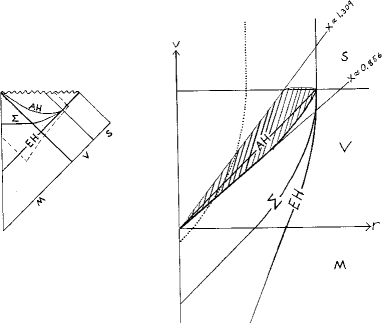
Figure 7: A Penrose diagram of a Vaidya spacetime, and a $v-r$ diagram of the region inside the dashed curve. It includes a part of the event horizon (EH), the spacelike part of the apparent 3-horizon (AH), and a hypersurface $\Sigma$ below which no trapped surfaces can extend [33]. The tongues discussed in the text are confined between two lines of constant $v/r$. There are also trapped surfaces to the left of the dotted curve.

The inequality that guarantees that the tongues are trapped is an unwieldy one, even in this simple case, and we had to rely partly on Mathematica in order to analyse it. For the case $\mu=1/2$ the answer is that the tongues remain trapped provided that

$$0.856<x=\frac{v}{r}<1.309\ .$$ (27)

This is how far a maximally extended trapped tongue, of this particular kind, extends—provided it stays in the Vaidya region, where the result in fact reflects the behaviour of trapped surfaces under homotheties [8]. If a tongue hits the Schwarzschild region there are further restrictions; see Fig. 7 for the final result, and Åman et al. [35] for other choices of $\mu$ and $a({\theta})$. The Gaussian curvature of this tongue is positive, and maximal at its “tips”. Its area grows as it extends more, at least to second order in a perturbation around a round sphere.

Of course this is a very naive construction. It would be more interesting to produce a marginally trapped tongue of this general type. Using general theorems [10, 7] one can prove [33] that they exist, and that they “evolve” into marginally trapped tubes intersecting the apparent 3-horizon, but to get them in explicit form seems to be very hard.

Can the trapped surfaces extend all the way into the flat region? Actually for sufficiently large $\mu$ the tongues we just discussed can do that, but let us try to design a surface that passes through the centre, also for $\mu=1/2$. We begin with the observation that locally trapped surfaces certainly exist in Minkowski space. A flat 2-plane has both its null expansions vanishing. So suppose we define a surface by setting

$$\theta=\frac{\pi}{2}\ ,\hskip 28.45274ptv=v(r)\ .$$ (28)

In the flat region this is marginally trapped if $t=v-r=$ constant. The idea is to “steer” it through the Vaidya region in such a way that it remains marginally trapped there, and see what it looks like when it emerges into the Schwarzschild region.

With our simple choice for the mass function it is easy to show that the surface remains minimal throughout the Vaidya region if we let $v(r)$ be a solution of the differential equation

$$\frac{dv}{dr}=\frac{1}{1-\frac{\mu v}{r}}\ .$$ (29)

We join this surface to the flat 2-plane in the flat region and find that its differentiability, in these coordinates, is $C^{2-}$. On the boundary to the Schwarzschild region it forms a round circle. Now it is interesting to observe that the cylindrical Schwarzschild surface

$$\theta=\frac{\pi}{2}\ ,\hskip 22.76219ptr=M\ ,$$ (30)

has both its null expansions vanishing, and it can be joined to one of the surfaces that we have steered through the Vaidya region by a suitable choice of integration constants. The result is a surface which is minimal throughout the entire spacetime—but its topology is that of a sphere with a point removed “at” the singularity, so this is not a closed marginally trapped surface.

But we can wiggle the surface a little bit, so that it becomes locally trapped, and so that it arrives to the Schwarzschild region with negative slope in the $v-r-$diagram. Continuing into Schwarzschild with fixed slope the null expansions become increasingly negative, and once they are sufficiently negative we can close off the surface with a spherical cap—we have constructed a closed trapped surface that extends into the flat part of the Vaidya spacetime. (Full details, for almost the same construction, can be found elsewhere [34].)

On the one hand this looks odd—one might have thought that no closed trapped surfaces could enter the flat region. But indeed in order to see that they are closed one has to collect information from a much larger region of spacetime. From another point of view it is somehow satisfactory, because it means that one cannot reach the singularity without crossing a trapped surface. Actually one can prove [33] that it is impossible for a trapped surface to enter the flat region if $\mu\leq 1/8$. But the smaller one makes $\mu$ the closer one gets to a nakedly singular spacetime, so that is presumably at the unphysical end.

A more systematic search for marginally trapped surfaces in the Vaidya solution, using a different mass function, an axisymmetric slicing, and a horizon finder, has been made by Nielsen et al. [36]. A more systematic study of spherically symmetric spacetimes in general will be found in Senovilla’s chapter in this book.

If we are content with outer trapped surfaces a different picture emerges. Then a trapped surface in the deep interior of the Schwarzschild region can develop a “tendril” reaching down through the Vaidya region and indeed through any point in the interior of the black hole, also in the flat diamond [37]. Once it emerges into the flat region the tendril lies in a tubular neighbourhood of a (null) generator of the event horizon. Casual inspection in the flat region would suggest that the tendril is part of an untrapped surface with its inner expansion negative, but in fact when the global structure of the spacelike slice is examined one sees that it is outer trapped. This behaviour was suggested by Eardley, who in fact conjectured that the boundary of the region through which outer trapped surfaces pass is always the event horizon, in any black hole [46].

What prevents the tendril from following its generator even further, out of the event horizon? The answer is that should it do so, it would no longer be lying in a suitable spacelike hypersurface, and would not count as “outer” any more. Indeed we assume it to be embedded in a spacelike hypersurfaces containing the trapped surface from which the tendril emerged in the first place. See Fig. 8. The lesson is that we can decide whether a surface is trapped by inspection of the surface itself, while this is not possible for outer trapped surfaces.

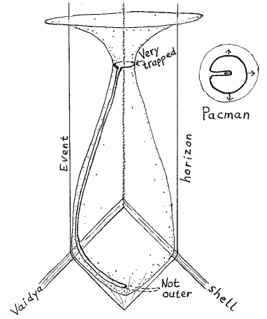
Figure 8: An impressionistic picture—$v$-$r$-coordinates would not be so useful here—of Ben-Dov’s construction [37]. A spacelike hypersurface sits inside the Vaidya event horizon, and it contains a very trapped surface around its “neck”, close to the singularity. This surface has developed a “tendril” reaching down to Minkowski space. It remains outer trapped, as one can see by flattening the spacelike hypersurface (at right). As far as the intrinsic properties of the tendril are concerned, they remain the same if the tendril extends outside the event horizon (shown dashed), but then no spacelike hypersurface can contain both the tip of the tendril and the very trapped surface from which it came.

7. Envoi

We hope that the reader enjoyed these examples. If not, the list of references will provide more satisfying reading. Meanwhile the examples may perhaps serve to drive home the point that being trapped or outer trapped is a spatially non-local property of a surface—and also that the condition for being outer trapped is substantially easier to fulfill.

8: Acknowledgments

I thank José Senovilla for a very enjoyable collaboration, Emma Jakobsson for permission to include some results from her Master’s thesis, and the Swedish Research Council for support under contract VR 621-2010-4060.

References

- [1] J. Thornburg, Event and apparent horizon finders for 3+1 numerical relativity, Living Rev. Relativity 10 (2007) 3; http:// www.livingreviews.org/lrr-2007-3.
- [2] S. W. Hawking and G. F. R. Ellis: The large scale structure of space-time, Cambridge UP, 1973.
- [3] R. P. A. C. Newman, Topology and stability of marginal 2-surfaces, Class. Quant. Grav. 4 (1987) 277.
- [4] M. Kriele and S. A. Hayward, Outer trapped surfaces and their apparent horizon, J. Math. Phys. 38 (1997) 1593.
- [5] M. Mars and J. M. M. Senovilla, Trapped surfaces and symmetries, Class. Quant. Grav. 20 (2003) L293.
- [6] M. Eichmair, The Plateau problem for marginally trapped surfaces, eprint arXiv:0711.4139, J. Diff. Geom, to appear.
- [7] L. Andersson and J. Metzger, The area of horizons and the trapped region, Commun. Math. Phys. 290 (2009) 941.
- [8] A. Carrasco and M. Mars, Stability in marginally outer trapped surfaces in spacetimes with symmetries, Class. Quant. Grav. 26 (2009) 175002.
- [9] A. Ashtekar and G. J. Galloway, Some uniqueness results for dynamical horizons, Theor. Math. Phys. 9 (2005) 1.
- [10] L. Andersson, M. Mars, and W. Simon, The time evolution of marginally trapped surfaces, Class. Quant. Grav. 26 (2009) 085018.
- [11] D. Christodoulou: The formation of black holes in general relativity, Monographs in Mathematics, EMS 2009.
- [12] F. J. Tipler, Black holes in closed universes, Nature 270 (1977) 500.
- [13] S. A. Hayward, General laws of black-hole dynamics, Phys. Rev. D49 (1994) 6467.
- [14] A. Ashtekar and B. Krishnan, Isolated and dynamical horizons and their applications, Living Rev. Relativity 7 (2004) 10; http://www.livingreviews.org/lrr-2004-10.
- [15] I. Booth, Black hole boundaries, Can. J. Phys. 83 (2005) 1073.
- [16] D. R. Brill and R. W. Lindquist, Interaction energy in geometrostatics, Phys. Rev. 131 (1963) 471.
- [17] C. W. Misner, The method of images in geometrostatics, Ann. Phys. 24 (1963) 102.
- [18] G. W. Gibbons, The time symmetric initial value problem for black holes, Commun. Math. Phys. 27 (1972) 87.
- [19] A Čadež, Apparent horizons in the two-black-hole problem, Ann. Phys. 83 (1974) 449.
- [20] N. T. Bishop, The closed trapped region and the apparent horizon of two Schwarzschild black holes, Gen. Rel. Grav. 14 (1982) 717.
- [21] M. Bañados, C. Teitelboim, and J. Zanelli, The black hole in three-dimensional space-time, Phys. Rev. Lett. 69 (1992) 1849.
- [22] S. Åminneborg and I. Bengtsson, Anti-de Sitter quotients: When are they black holes?, Class. Quant. Grav. 25 (2008) 095019.
- [23] D. R. Brill, Multi-black-hole geometries in (2+1)-dimensional gravity, Phys. Rev. D53 (1996) 4133.
- [24] A. Steif, Time-symmetric initial data for multi-body solutions in three dimensions, Phys. Rev. D53 (1996) 5527.
- [25] S. Åminneborg, I. Bengtsson, D. R. Brill, S. Holst, and P. Peldán, Black holes and wormholes in 2 + 1 dimensions, Class. Quant. Grav. 15 (1998) 627.
- [26] E. Jakobsson, Trapped surfaces in 2 + 1 dimensions, Master’s Thesis, Stockholm Univ., 2011.
- [27] S. Holst and P. Peldán, Black holes and causal structure in anti-de Sitter isometric spacetimes, Class. Quant. Grav. 14 (1997) 3433.
- [28] R. Penrose, Naked singularities, Ann. N. Y. Acad. Sci. 224 (1973) 125.
- [29] K. P. Tod, Penrose’s quasi-local mass and the isoperimetric inequality for static black holes, Class. Quant. Grav. 2 (1985) L65.
- [30] G. W. Gibbons, The isoperimetric and Bogomolny inequalities for black holes, in T. J. Willmore and N. J. Hitchin (eds.): Global Riemannian Geometry, Ellis Horwood, Chichester 1984.
- [31] M. A. Pelath, K. P. Tod, and R. M. Wald, Trapped surfaces in prolate collapse in the Gibbons-Penrose construction, Class. Quant. Grav. 15 (1998) 3917.
- [32] A. Papapetrou, Formation of a singularity and causality, in N. Dadhich et al. (eds): A Random Walk in Relativity and Cosmology, Wiley 1985.
- [33] I. Bengtsson and J. M. M. Senovilla, The region with trapped surfaces in spherical symmetry, its core, and its boundary, Phys. Rev. D83 (2011) 044012.
- [34] I. Bengtsson and J. M. M. Senovilla, A note on trapped surfaces in the Vaidya solution, Phys. Rev. D79 (2009) 024027.
- [35] J. E. Åman, I. Bengtsson, and J. M. M. Senovilla, Where are the trapped surfaces?, J. Phys.: Conf. Ser. 229 (2010) 012004.
- [36] A. B. Nielsen, M. Jasiulek, B. Khrishnan, and E. Schnetter, The slicing dependence of non-spherically symmetric quasi-local horizons in Vaidya spacetimes, Phys. Rev. D83 (2011) 124022.
- [37] I. Ben-Dov, Outer trapped surfaces in Vaidya spacetimes, Phys. Rev. D75 (2007) 064007.
- [38] J. Plateau, Sur les figures d’equilibre d’une masse liquide sans pésanteur, Mém. Acad. Roy. Belgique Vol 23 (1849).
- [39] H. B. Lawson: Lectures on Minimal Submanifolds Vol I, Publish or Perish, Berkeley 1980.
- [40] H. B. Lawson, Compact minimal surfaces in , in Proc. Symp. Pure Mathematics Vol. XV, AMS, Providence 1970.
- [41] G. T. Horowitz, The positive energy theorem and its extensions, in E. J. Flaherty (ed.): Asymptotic Behavior of Mass and Spacetime Geometry, Springer, Berlin 1984.
- [42] I. Ben-Dov, Penrose inequality and apparent horizons, Phys. Rev. D70 (2004) 124031.
- [43] S. Holst, Horizons and time machines, PhD thesis, Stockholm Univ., 2000.
- [44] S. Deser, R. Jackiw, and G. ’tHooft, Three-dimensional Einstein gravity: Dynamics of flat space, Ann. Phys. 152 (1984) 220.
- [45] R. M. Wald and V. Iyer, Trapped surfaces in the Schwarzschild geometry and cosmic censorship, Phys. Rev. D44 (1991) R3719.
- [46] D. M. Eardley, Black hole boundary conditions and coordinate conditions, Phys. Rev. D54 (1996) 4862.