Abstract.  The dynamics of metric perturbations is explored in the gravity theory with anomaly-induced quantum corrections. Our first purpose is to derive the equation for gravitational waves in this theory on the general homogeneous and isotropic background, and then verify the stability of such background with respect to metric perturbations. The problem under consideration has several interesting applications. Our first purpose is to explore the stability of the classical cosmological solutions in the theory with quantum effects taken into account. There is an interesting literature about stability of Minkowski and de Sitter spaces and here we extend the consideration also to the radiation and matter dominated cosmologies. Furthermore, we analyze the behavior of metric perturbations during inflationary period, in the stable phase of the Modified Starobinsky inflation.

Keywords:  Conformal anomaly,  quantum effects,  stability,  cosmological solutions,  gravitational waves.
PACS:  04.62.+v, 98.80.-k, 04.30.-w
AMS:  83F05,   81V17,   83D05

1 Introduction

The semiclassical approach to gravity is usually associated with the equation

$$G_{\mu\nu}\,=\,R_{\mu\nu}-\frac{1}{2}\,Rg_{\mu\nu}\,=\,<T_{\mu\nu}>$$ (1)

and implies that the gravity itself is not quantized. The averaging in the r.h.s. of the last equation comes from the quantum matter fields. Different from what one can think, the r.h.s. may be very nontrivial even if no matter sources are present in the given point of space-time. The reason is that the average of the Energy-Momentum tensor of the vacuum can be nontrivial, for it may depend on the curvature tensor components and its derivatives, with possible non-local structures. There are two subtle points in the equation (1). Let us start from the terminology. The renormalizable theory of matter fields on curved space-time background requires that the action of gravity should be extended compared to the one of General Relativity (GR) [1, 2, 3] (see also [4] for the recent review). The full action includes Einstein-Hilbert term, which is the origin of the r.h.s. of (1) with the cosmological constant term

$$S_{EH}\,=\,-\,\frac{1}{16\pi G}\int d^{4}x\sqrt{-g}\,\left(\,R+2\Lambda\,\right)$$ (2)

and also the higher derivative terms

$$S_{HD} = \int d^{4}x\sqrt{-g}\left\{a_{1}C^{2}+a_{2}E+a_{3}{\Box}R+a_{4}R^{2}\right\},$$ (3)

where $\,C^{2}=R_{\mu\nu\alpha\beta}^{2}-2R_{\alpha\beta}^{2}+(1/3)\,R^{2}\,$ is the square of the Weyl tensor and $\,E=R_{\mu\nu\alpha\beta}^{2}-4R_{\alpha\beta}^{2}+R^{2}\,$ is the integrand of the Gauss-Bonnet topological term. All terms of the action of vacuum

$$S_{vac} = S_{EH}\,+\,S_{HD}\,,$$ (4)

belong to the gravitational action. If we consider the Einstein equations as something intended to define the relation between geometry and distribution of matter, it is clear that the whole $S_{vac}$ should contribute to the l.h.s. of (1). However, by traditional virtue we use to put all the contributions beyond the Einstein tensor to the r.h.s.. To a great extent this way of settling the terms is explained by the fact that Eq. (1) with the  classical  Energy-Momentum tensor at the r.h.s. work pretty well and provide very good fit for many observational tests of GR. So, it looks like all extra terms, except the cosmological constant, are in fact unnecessary at the classical level and therefore their introduction is no justified in a purely gravitational framework. In other words, why should the gravitational physicist who works with the very large scale phenomena, worry about the quantum notions, such as renormalizability? In fact, the use of the terms (3) may lead to serious problems, because these terms are known to produce unphysical ghost terms for the linearized gravitational field on the flat background [5]. So, it is somehow unclear how to apply the consistent at quantum level theory (4) for the classical gravitational purposes.

Another aspect of the same problem is related to quantum corrections to (4). In general, the problem of deriving such corrections is unsolved, but there is one important case where the situation is quite clear. The one-loop effective action of massless conformal fields is essentially controlled by conformal anomaly [6]. Indeed, the anomaly-induced effective action of vacuum includes an arbitrary conformal functional, but in many particular cases its role is known to be very restricted. For instance, this functional is a trivial constant for the homogeneous and isotropic metric, where the anomaly-induced quantum corrections produce Starobinsky inflation [7]. In the case of black holes, taking into account the conformal anomaly enables one to calculate Hawking radiation [8] and using the anomaly-induced action one can even classify the vacuum states in the vicinity of the black hole [9, 10]. The equations for gravitational waves calculated by using direct methods [11, 12] and anomaly-induced action [13] produce equivalent results at least on the de Sitter background. In both last cases the mentioned conformal functional apparently plays no role, which can be explained by the fact that the conformal anomaly picks up all quantum effects which correspond to the UV limit and, therefore, the remaining terms can be relevant only for the sub-leading effects. So, from the Quantum Field Theory viewpoint the anomaly-induced effective action of vacuum represents a well-defined quantum contribution which can be used to verify the compatibility of gravity and quantum effects in the sense we have discussed above. The late Universe represents, in fact, a very good opportunity for such a verification. The typical energy scale of gravity is given by the Hubble parameter or by the scale of the gravitational waves, both of which are much smaller than the masses of all quantum massive fields. Certainly, all such fields strongly decouple in the higher derivative sector of the theory [14] and therefore the only active quantum field is photon. So, we arrive at the conclusion that the anomaly-induced action of vacuum coming from the photon field is a safe approximation for the quantum contribution in the late Universe. The purpose of the present work is to verify whether these quantum terms are compatible with the well-known classical cosmological solutions for the different epochs of the history of the Universe. The method which will be used in what follows is based on the derivation of metric perturbations over the given cosmological solution, in the theory with anomaly-induced effective action of gravity.

The investigation of stability of the physically important solutions in a more general gravitational theories has a long and interesting history, starting from [15], where the stability of Minkowski quantum vacuum has been explored for the first time (see also [16]). Similar program for the theory of quantum gravity at non-zero temperature has been carried out in [17]. The stability of Minkowski has been further studied in [18]. The stability of de Sitter space for both semiclassical theory and quantum gravity, within different quantization schemes has been recently considered in [19]. Furthernmore, the stability of de Sitter space has been recently discussed in [20] by an unconventional method of power counting in the IR limit, with an apparently negative result concerning the validity of the whole semiclassical approximation (see further references therein). Compared to the methods of exploring stability used in the papers mentioned above, the anomaly-induced effective action has two important advantages: safety and simplicity. As we have already mentioned above, the anomaly-induced action is picks up the most important non-local part of effective action. As far as it is based on the conformal anomaly of massless fields, it is closely related to both UV and IR limits of the theory and hence is independent on whether we use usual in-out or more complicated in-in formalism. Also (see next section) the anomaly-induced action is very simple, it is given by a compact and explicit non-local expression which can be easily made local by introducing two auxiliary scalar fields. Historically, the anomaly-induced effective action was the theoretical basis of the first cosmological models with quantum corrections [21], Starobinsky inflation [7] and first derivation of cosmic perturbations in inflationary model [22]. As we will see below, the use of anomaly-induced action enables one to explore stability not only for Minkowski or de Sitter spaces, but for a wider set of classical cosmological solutions.

In our investigation of stability we will restrict consideration by the gauge invariant part of metric perturbations related to the gravitational wave. The solutions of our interest include the radiation and matter - dominated Universes, the late Universe dominated by the cosmological constant and the stable phase of the modified Starobinsky inflation [23, 24].

The paper is organized as follows. In Sect. 2 present a brief review of anomaly-induced action of gravity and of the corresponding cosmological solutions. Sect. 3 is devoted to the derivation of gravitational waves equation on an arbitrary cosmological (homogeneous and isotropic) background. In Sect. 4 we explore the stability of classical solutions by means of approximate analytic method and in Sect. 5 discuss the spectrum of metric perturbations. Sect. 6 is about the behavior of gravitational waves in the Modified Starobinsky model of inflation. Finally, in the last section we draw our conclusions.

2 Effective action induced by anomaly

The covariant form of anomaly-induced effective action of gravity [25, 26] is the most complete available form of the quantum corrections to the gravitational action in four space-time dimensions. The application to cosmology has been considered in [21, 27] and led to the well-known Starobinsky model of inflation [7] (see also more detailed description in [28] and consequent development in form of Modified Starobinsky model [23, 24]).

The anomalous trace of the energy momentum tensor is given by the expression [6, 2]

$$<T_{\mu}^{\mu}>\,=\,-\,(wC^{2}+bE+c{\Box}R)\,,$$ (5)

where the coefficients $w,b$ and $c$ depend on the number of active quantum fields of different spins,

$$w = \frac{1}{(4\pi)^{2}}\,\Bigg{(}\frac{N_{0}}{120}+\frac{N_{1/2}}{20}+\frac{N_{1}}{10}\Bigg{)}\,,$$ (6)

$$b = -\,\frac{1}{(4\pi)^{2}}\,\Bigg{(}\frac{N_{0}}{360}+\frac{11\,N_{1/2}}{360}+\frac{31\,N_{1}}{180}\Bigg{)}\,,$$ (7)

$$c = \frac{1}{(4\pi)^{2}}\,\Bigg{(}\frac{N_{0}}{180}+\frac{N_{1/2}}{30}-\frac{N_{1}}{10}\Bigg{)}\,.$$ (8)

It is easy to see that these coefficients are nothing else but the $\beta$-functions for the parameters $a_{1,2,3}$ in the classical action of vacuum (4). Due to the decoupling phenomenon [14], the number of active fields can vary from one epoch in the history of the Universe to another. As we have already mentioned in the Introduction, the present-day Universe corresponds to the particle content with $\,N_{0}=N_{1/2}=0\,$ and $\,N_{1}=1$.

The anomaly-induced effective action ${\bar{\Gamma}}_{ind}$ represents an addition to the classical action of gravity, and can be found by solving the equation

$$\frac{2}{\sqrt{-g}}\,g_{\mu\nu}\frac{\delta\,{\bar{\Gamma}}_{ind}}{\delta g_{\mu\nu}}\,=\,<T_{\mu}^{\mu}>\,=\,(\omega C^{2}+bE+c{\Box}R)\,.$$ (9)

The covariant and generally non-local solution can be easily found in the form

$${\bar{\Gamma}} = S_{c}[g_{\mu\nu}]\,-\,\frac{3c+2b}{36}\,\int d^{4}x\sqrt{-g(x)}\,R^{2}(x)$$

⁺ $$\int d^{4}x\sqrt{-g(x)}\,\int d^{4}y\sqrt{-g(y)}\,(E-\frac{2}{3}{\Box}R)_{x}\,G(x,y)\,\left[\,\frac{w}{4}\,C^{2}-\frac{b}{8}\,(E-\frac{2}{3}{\Box}R)\right]_{y}\,,$$

where $\,G(x,y)\,$ is a Green function for the operator

$$\Delta_{4}={\Box}^{2}+2\,R^{\mu\nu}\nabla_{\mu}\nabla_{\nu}-\frac{2}{3}\,R{\Box}+\frac{1}{3}\,(\nabla^{\mu}R)\nabla_{\mu}\,.$$

Finally, one can rewrite (2) in the local form by introducing two auxiliary fields $\phi$ and $\psi$ [29] (see also [30] for an alternative albeit equivalent scheme),

$${\bar{\Gamma}}_{ind} = S_{c}[g_{\mu\nu}]-\frac{3c+2b}{36}\,\int d^{4}x\sqrt{-g(x)}\,R^{2}(x)+\int d^{4}x\sqrt{-g(x)}\,\Big{\{}\frac{1}{2}\varphi\Delta_{4}\varphi-\frac{1}{2}\psi\Delta_{4}\psi$$ (11)

$$+ \varphi\,\Big{[}\,\frac{\sqrt{-b}}{2}\,\big{(}E-\frac{2}{3}\,{\Box}R\big{)}\,-\frac{w}{2\sqrt{-b}}\,C^{2}\,\Big{]}+\frac{w}{2\sqrt{-b}}\,\psi\,C^{2}\Big{\}}\,.$$

The expression (11) is classically equivalent to (2), because if one uses the equations for the auxiliary fields $\,\varphi\,$ and $\,\psi$, the nonlocal action (2) is restored. Consider now the background cosmological solution for the theory with the action including quantum corrections,

$$S_{total}\,=\,-\,M^{2}_{P}\,\int d^{4}x\,\sqrt{-g}\,R\,+\,{\bar{\Gamma}}\,,$$ (12)

where $M^{2}_{P}={1}/{16\pi G}$ is the square of the Planck mass, and the quantum correction $\,{\bar{\Gamma}}\,$ is taken in the form (11).

Looking for the isotropic and homogeneous solution, the starting point is to choose the metric in the form $g_{\mu\nu}=a^{2}(\eta)\,{\bar{g}}_{\mu\nu}$, where $\,\eta\,$ is conformal time. It proves useful to introduce the notation $\,\sigma=\,\mbox{ln}\,a$. The theory includes the equations for the three fields, namely for $\,\varphi,\,\psi,\,$ and $\,\sigma$. For the sake of simplicity we will consider conformally flat background and therefore set $\,{\bar{g}}_{\mu\nu}=\eta_{\mu\nu}$.

Equations for $\,\varphi\,$ and $\,\psi\,$ have especially simple form

$$\sqrt{-g}\,\left[\,\Delta_{4}\,\varphi+\frac{\sqrt{-b}}{2}\,(E-\frac{2}{3}\,{\Box}R)\,-\frac{w}{2\sqrt{-b}}\,C^{2}\,\right]=0\,,$$

$$\sqrt{-g}\,\left[\,\Delta_{4}\,\psi-\frac{w}{2\sqrt{-b}}\,C^{2}\,\right]=0\,.$$

By using the transformation laws for the quantities in the last expression, one can obtain

$$\sqrt{-g}C^{2}=\sqrt{-{\bar{g}}}{\bar{C}}^{2}\,,\,\,\,\,\,\,\,\,\,\,\,\,\,\,\,\,\,\,\sqrt{-{g}}\,{\Delta}_{4}=\sqrt{-{\bar{g}}}\,{\bar{\Delta}}_{4}\,\,,$$ (13)

$$\sqrt{-g}(E-\frac{2}{3}{\Box}R)=\sqrt{-{\bar{g}}}({\bar{E}}-\frac{2}{3}{\bar{\Box}}{\bar{R}}+4{\bar{\Delta}}_{4}\sigma)\,.$$ (14)

Taking into account our choice for the fiducial metric $\,{\bar{g}}_{\mu\nu}=\eta_{\mu\nu}$ all the terms in the r.h.s. of the last equation are equal to zero and we arrive at the following equations

$${\Box}^{2}\,\varphi+8\pi\sqrt{-b}\,{\Box}^{2}\sigma=0\,,\,\,\,\,\,\,\,\,\,\,\,\,\,\,\,\,\,\,\,\,\,{\Box}^{2}\,\psi=0\,.$$ (15)

The solutions of (15) can be presented in the form

$$\varphi=-8\pi\sqrt{-b}\,\sigma+\varphi_{0}\,,\,\,\,\,\,\,\,\,\,\,\,\,\,\,\,\,\,\,\,\,\,\psi=\psi_{0}\,.$$ (16)

where $\Box$ is the flat-space D’Alembertian and $\varphi_{0},\,\psi_{0}$ are general solutions of the homogeneous equations $\,{\Box}^{2}\,\varphi_{0}=0\,,\,\,\,{\Box}^{2}\,\psi_{0}=0.\,$

There is an obvious arbitrariness related to the choice of the initial conditions for the auxiliary fields $\varphi,\,\psi$. However, replacing Eq. (16) back into the action and taking variation with respect to $\sigma$ we arrive at the unique equation for $\sigma$. It proves useful to write this equation in terms of $a(t)$ and the physical time $t$, with derivatives denoted by points. Another useful variable is of course the Hubble parameter, $H(t)={\dot{a}}(t)/a(t)={\dot{\sigma}}(t)$. Then, we obtain

$$\frac{{\stackrel{{\scriptstyle....}}{{a}}}}{a}+\frac{{3\stackrel{{\scriptstyle.}}{{a}}}{\stackrel{{\scriptstyle...}}{{a}}}}{a^{2}}+\frac{{\stackrel{{\scriptstyle..}}{{a}}}^{2}}{a^{2}}-\left(5+\frac{4b}{c}\right)\frac{{\stackrel{{\scriptstyle..}}{{a}}}{\stackrel{{\scriptstyle.}}{{a}}}^{2}}{a^{3}}-2k\left(1+\frac{2b}{c}\right)\frac{{\stackrel{{\scriptstyle..}}{{a}}}}{a^{3}}$$

$$-\frac{M_{P}^{2}}{8\pi c}\left(\frac{{\stackrel{{\scriptstyle..}}{{a}}}}{a}+\frac{{\stackrel{{\scriptstyle.}}{{a}}}^{2}}{a^{2}}-\frac{2\Lambda}{3}\right)\,=\,-\,\frac{\rho^{0}_{m}}{c\,a^{3}}\,.$$ (17)

In the r.h.s. of the last equation we have included the contribution of matter with constant $\rho_{m}$ and explicitly shown dependence on $a(t)$. As far as we deal with the trace of the generalized Einstein equations (linear combination of generalized Friedmann equations), the contribution of radiation does not show up, but it can be easily restored if we switch to an equivalent $(00)$-component [21, 12, 7].

There are several relevant observations we have to make about the solutions of Eq. (17) in different physical situations. First of all, in the theory without matter, when $\rho_{m}=0$, there are two exact solutions, namely

$$a(t)\,=\,a_{0}\cdot\exp(Ht)$$ (18)

where [24]

$$H\,=\,\frac{M_{P}}{\sqrt{-32\pi b}}\,\left(1\pm\sqrt{1-\frac{64\pi b}{3}\frac{\Lambda}{M_{P}^{2}}}\right)^{1/2}.$$ (19)

As far as the cosmological constant is quite small compared to the square of the Planck mass, $\,\Lambda\ll M_{P}^{2}$, we meet two very different values of $H$ (here $\Lambda>0$)

$$H_{c}\,\approx\,\sqrt{\frac{\Lambda}{3}}\,\,\,\,\,\,\,\,\,\,\,\,{\rm and}\,\,\,\,\,\,\,\,\,\,\,\,H_{S}\,\approx\,\frac{M_{P}}{\sqrt{16\pi b}}\,.$$ (20)

It is easy to see that the first solution with $H_{c}$ is the one of the theory without quantum corrections, while the second value $\,H_{S}\,$ corresponds to the inflationary solution of Starobinsky [7]. The sign of $\,b\,$ is always negative, independent on the particle content, see Eq. (7). Let us remark that the particle content which we deal with here, $\,N_{0},\,N_{1/2}\,$ and $\,N_{1}\,$, corresponds to the degrees of freedom contributing to the vacuum effective action and has nothing to do with the real matter content of the universe.

Second, the stability properties of the solutions (20) depend on the sign of the coefficient $\,c$, that is on the coefficient of the local $\,\int\sqrt{-g}R^{2}$-term [7, 24]. The inflationary solution $H_{S}$ is stable for a positive $\,c\,$ and is unstable for $\,c<0$. The stability of the low-energy solution $H_{c}$ requires opposite sign relations for $c$. It was shown in [24] that the $H_{c}$ solution with $\,c<0$ is stable with respect to the small variations of the Hubble parameter (or, equivalently, of $\sigma(t)$). In the original Starobinsky model of inflation [7] the particles content corresponds to the unstable inflation and the initial data is chosen such that the Universe is asymptotically approaching the radiation-dominated FRW solution. In order to better understand the situation, let us replace the corresponding FRW solution, e.g., $a(t)\sim t^{2/3}$, into the equation (17). It is easy to see that the classical part, composed by Einstein and matter terms, do behave like $1/t^{2}$, while the quantum corrections, which are given by higher derivative terms, behave like $1/t^{4}$. This means that in the unstable phase the quantum terms do decay rapidly, such that the classical solution $a(t)\sim t^{2/3}$ is an excellent approximation to the solution of Eq. (17) in the corresponding epoch. It is an easy exercise to check that the same is true for the radiation-dominated $a(t)\sim t^{1/2}$ and cosmological constant-dominated epochs too. An alternative form of these considerations can be found in [31]. Indeed, all the arguments presented above are valid for the dynamics of the conformal factor only. The next sections will be devoted to the stability of the same classical solutions with respect to the tensor metric perturbations (which we identify, for brevity, as gravitational waves). In the theory with quantum terms such as (4) and (11), the equations for the gravitational wave have fourth derivatives and hence they represent a real danger for stability of the classical solutions.

In the modified version of Starobinsky inflation [23, 24] the Universe starts with the stable inflation, that can be provided by choosing the supersymmetric particle content $\,N_{0},\,N_{1/2}\,$ and $\,N_{1}\,$. Then the exponential inflation slows down due to the quantum effects of matter fields (mainly $s$-particles) and at some point the heavy $s$-particles decouple from gravity and then the Universe starts the unstable inflationary phase. The advantage of this version is that it does not depend on the choice of initial conditions. The stability of the stable inflation with respect to the metric perturbations will be explored in Sect. 6.

3 Derivation of the gravitational waves

Let us derive the equation for the tensor modes of metric perturbations. First we rewrite the action in a more appropriate way and then derive linear perturbations for the tensor mode.

3.1 Total action with quantum terms

It proves useful to present the action (12) of a more useful way. After performing some integrations by parts, it can be cast into the form

$$S\,=\,\int\,d^{4}x\,L\,,$$ (21)

with

$$L\,=\,\sum^{5}_{s\,=\,0}\,f_{s}\,L_{s}$$

$$= \sqrt{-g}\,\Big{[}f_{0}\,R+f_{1}\,R^{\alpha\beta\mu\nu}R_{\alpha\beta\mu\nu}+f_{2}\,R^{\alpha\beta}R_{\alpha\beta}+f_{3}\,R^{2}+f_{4}\,\varphi\Box R+f_{5}\,\varphi\Delta\varphi\Big{]}\,,$$

where the $f$-terms are defined as

$$f_{0}\, = \,-\frac{{M_{P}}^{2}}{16\pi}\,;$$ (23)

$$f_{1}\, = \,a_{1}+a_{2}-\frac{b+\omega}{2\sqrt{-b}}\,\varphi+\frac{\omega}{2\sqrt{-b}}\,\psi;$$ (24)

$$f_{2}\, = \,-2a_{1}-4a_{2}+\frac{\omega+2b}{\sqrt{-b}}\,\varphi-\frac{\omega}{\sqrt{-b}}\,\psi;$$ (25)

$$f_{3}\, = \,\frac{a_{1}}{3}+a_{2}-\frac{3c+2b}{36}-\frac{3b+\omega}{6\sqrt{-b}}\,\varphi+\frac{\omega}{6\sqrt{-b}}\,\psi;$$ (26)

$$f_{4}\, = \,-\frac{4\pi\sqrt{-b}}{3};$$ (27)

$$f_{5}\, = \,\frac{1}{2}\,,$$ (28)

where the coefficients $a_{1,2}$ are the same defined in (4).

3.2 Perturbation equations

Using the conditions (with $\mu\,=\,0,1,2,3$ and $i\,=\,1,2,3$),

$$\partial_{i}\,h^{ij}\,=\,0\,\,\,\mbox{and}\,\,\,h_{kk}\,=\,0\,,$$ (29)

together with the synchronous coordinate condition $h_{\mu 0}\,=\,0$, we introduce metric perturbation in the equation (3.1) as follows

$$g_{\mu\nu}\,=\,g_{\mu\nu}^{0}+h_{\mu\nu}\,,\,\,\,\,\,h_{\mu\nu}\,=\,\delta\,g_{\mu\nu}\,.$$ (30)

Here $g_{\mu\nu}^{0}\,=\,\{1,-\delta_{ij}\,a^{2}(t)\}$ are the background cosmological solutions. In this way one can arrive at the following expressions for the bilinear parts of the partial Lagrangians from Eq. (3.1):

$$L_{0}\, = \,a^{3}\,f_{0}\Big{[}h^{2}\Big{(}\frac{3}{2}\dot{H}+3H^{2}\Big{)}+h\ddot{h}+4Hh\dot{h}+\frac{3}{4}\dot{h}^{2}-\frac{h}{4}\frac{\nabla^{2}h}{a^{2}}\Big{]}+{\cal O}(h^{3}),$$

$$L_{1}\, = \,a^{3}\,f_{1}\Big{[}{\dot{h}}^{2}\Big{(}2H^{2}-2\dot{H}\Big{)}-h\ddot{h}\Big{(}4H^{2}+4\dot{H}\Big{)}-h^{2}\Big{(}3\dot{H}^{2}+6\dot{H}H^{2}+6H^{4}\Big{)}-$$

$$- h\dot{h}\Big{(}8H\dot{H}+16H^{3}\Big{)}+\ddot{h}^{2}+4H\dot{h}\ddot{h}+\Big{(}\frac{\nabla^{2}h}{a^{2}}\Big{)}^{2}+2\dot{h}\frac{\nabla^{2}\dot{h}}{a^{2}}+$$

$$+ \Big{(}H^{2}h-2H\dot{h}\Big{)}\frac{\nabla^{2}h}{a^{2}}\Big{]}+{\cal O}(h^{3}),$$

$$L_{2}\, = \,a^{3}\,f_{2}\Big{[}-h\dot{h}\Big{(}12\dot{H}H+24H^{3}\Big{)}-\frac{\dot{h}^{2}}{2}\Big{(}5\dot{H}+\frac{18}{4}H^{2}\Big{)}-$$

$$- h^{2}\Big{(}3\dot{H}^{2}+9\dot{H}H^{2}+9H^{4}\Big{)}-h\ddot{h}\Big{(}4\dot{H}+6H^{2}\Big{)}+\frac{\ddot{h}^{2}}{4}+\frac{3}{2}H\dot{h}\ddot{h}+$$

$$+ \frac{1}{4}\Big{(}\frac{\nabla^{2}h}{a^{2}}\Big{)}^{2}-\frac{1}{2}\Big{(}\ddot{h}+3H\dot{h}-\dot{H}h-3H^{2}h\Big{)}\frac{\nabla^{2}h}{a^{2}}\Big{]}+{\cal O}(h^{3}),$$

$$L_{3}\, = \,-6a^{3}\,f_{3}\Big{(}\dot{H}+2H^{2}\Big{)}\Big{[}h^{2}\Big{(}\frac{3}{2}\dot{H}+3H^{2}\Big{)}+2h\ddot{h}+$$

$$+ 8Hh\dot{h}+\frac{3}{2}\dot{h}^{2}-\frac{h}{2}\frac{\nabla^{2}h}{a^{2}}\Big{]}+{\cal O}(h^{3}),$$

$$L_{4}\, = \,a^{3}\,f_{4}\,\Big{[}\frac{3}{2}\Big{(}\dot{H}+2H^{2}\Big{)}\Big{(}\ddot{\varphi}+3H\dot{\varphi}\Big{)}h^{2}+\Big{(}\ddot{\varphi}+3H\dot{\varphi}\Big{)}h\ddot{h}+\Big{(}18H^{2}\dot{\varphi}+4H\ddot{\varphi}\Big{)}h\dot{h}+$$

$$+ \frac{3}{4}\Big{(}\ddot{\varphi}+3H\dot{\varphi}\Big{)}\dot{h}^{2}-\frac{1}{4}\Big{(}\ddot{\varphi}+3H\dot{\varphi}\Big{)}\frac{1}{a^{2}}h\nabla^{2}h\Big{]}+{\cal O}(h^{3}),$$

$$L_{5} = a^{3}\,f_{5}\,\Big{\{}\Big{[}\ddot{\varphi}h^{2}-\frac{3}{2}H\dot{\varphi}h^{2}-\dot{\varphi}\dot{h}h\Big{]}\ddot{\varphi}+$$ (31)

$$+ \dot{\varphi}^{2}\Big{[}-\frac{7}{4}H^{2}h^{2}-\frac{1}{4}\dot{H}h^{2}-\frac{7}{3}H\dot{h}h-\frac{1}{3}\ddot{h}h-\frac{1}{6}\frac{h}{a^{2}}\nabla^{2}h\Big{]}\Big{\}}+{\cal O}(h^{3}).$$

One can perform a comparison of these equations with the ones known from the literature. A very similar expansion was obtained by Gasperini in [32] in order to explore metric perturbations in the pre-Big-Bang inflationary scenario. Despite the physical motivations of the pre-Big-Bang inflation are quite different from our case, when we intend to consider the semiclassical gravity with the action induced by anomaly, the formulas are mainly equivalent and we find a perfect correspondence between our results and the ones of [32]. On the other hand, we can successfully compare part of the expressions presented above with our own previous calculation of the same equations for the $H=const$ case in [13].

In order to get the equation for linearized tensor perturbations, one has to omit all higher order terms ${\cal O}(h^{3})$ in the expressions (31) and then proceed by taking variational derivative with respect to $h_{\mu\nu}$. The next step is to use the solutions (16) for the auxiliary fields. We fix the ambiguity in these solutions by choosing the simplest zero option for the conformal terms which are not controlled by conformal anomaly and set  $\psi_{0}=\varphi_{0}=0$. As a consequence we have

$$\dot{\varphi}=-8\pi\sqrt{-b}\,H\,,\quad\ddot{\varphi}=-8\pi\sqrt{-b}\,{\dot{H}}\,,\quad\stackrel{{\scriptstyle...}}{{\varphi}}=-8\pi\sqrt{-b}\,{\ddot{H}}\quad\mbox{and}\quad\stackrel{{\scriptstyle....}}{{\varphi}}=-8\pi\sqrt{-b}\,\stackrel{{\scriptstyle...}}{{H}}.$$ (32)

These relations for the background must be replaced into the equations for tensor perturbations, but we prefer to keep $\varphi$-dependent form, for the sake of generality. After all, the equation for tensor mode can be cast into the form

$$\Big{(}2f_{1}+\frac{f_{2}}{2}\Big{)}\,\stackrel{{\scriptstyle....}}{{h}}+\Big{[}3H\Big{(}4f_{1}+f_{2}\Big{)}+4\dot{f_{1}}+\dot{f_{2}}\Big{]}\,\stackrel{{\scriptstyle...}}{{h}}+\Bigl{[}3H^{2}\Big{(}6f_{1}+\frac{f_{2}}{2}-4f_{3}\Big{)}$$ (33)

$$+ H\Big{(}16\dot{f_{1}}+\frac{9}{2}\dot{f_{2}}\Big{)}+6\dot{H}\Big{(}f_{1}-f_{3}\Big{)}+2\ddot{f_{1}}+\frac{1}{2}\big{(}\ddot{f_{2}}+f_{0}+f_{4}\ddot{\varphi}\big{)}+\frac{3}{2}f_{4}H\dot{\varphi}-\frac{2}{3}f_{5}\dot{\varphi}^{2}\Bigl{]}\,\ddot{h}$$

$$- \Big{(}4f_{1}+f_{2}\Big{)}\,\frac{\nabla^{2}\ddot{h}}{a^{2}}+\Big{[}\dot{H}\Big{(}4\dot{f_{1}}-6\dot{f_{3}}\Big{)}-21H\dot{H}\Big{(}\frac{1}{2}f_{2}+2f_{3}\Big{)}-\ddot{H}\Big{(}\frac{3}{2}f_{2}+6f_{3}\Big{)}$$

$$+ 3H^{2}\Big{(}4\dot{f_{1}}+\frac{1}{2}\dot{f_{2}}-4\dot{f_{3}}\Big{)}-9H^{3}\big{(}f_{2}+4f_{3}\big{)}+H\Big{(}4\ddot{f_{1}}+\frac{3}{2}\ddot{f_{2}}\Big{)}+\frac{3}{2}f_{4}\dot{\varphi}\Big{(}3H^{2}+\dot{H}\Big{)}$$

$$+ H\big{(}3f_{4}\ddot{\varphi}+\frac{3}{2}f_{0}-2f_{5}\dot{\varphi}^{2}\big{)}+\frac{1}{2}f_{4}\stackrel{{\scriptstyle...}}{{\varphi}}-\frac{4}{3}f_{5}\dot{\varphi}\ddot{\varphi}\Bigl{]}\,\dot{h}-\big{[}H\Big{(}4f_{1}+f_{2}\Big{)}+4\dot{f_{1}}+\dot{f_{2}}\big{]}\,\frac{\nabla^{2}\dot{h}}{a^{2}}$$

$$+ \Big{[}5f_{4}H\stackrel{{\scriptstyle...}}{{\varphi}}+f_{4}\stackrel{{\scriptstyle....}}{{\varphi}}-\big{(}36\dot{H}H^{2}+18\dot{H}^{2}+24H\ddot{H}+4\stackrel{{\scriptstyle...}}{{H}}\big{)}\Big{(}f_{1}+f_{2}+3f_{3}\Big{)}$$

$$- H\dot{H}\Big{(}32\dot{f_{1}}+36\dot{f_{2}}+120\dot{f_{3}}\Big{)}-8\ddot{H}\Big{(}\dot{f_{1}}+\dot{f_{2}}+3\dot{f_{3}}\Big{)}-H^{2}\Big{(}4\ddot{f_{1}}+6\ddot{f_{2}}+24\ddot{f_{3}}\Big{)}$$

$$- 4\dot{H}\Big{(}\ddot{f_{1}}+\ddot{f_{2}}+3\ddot{f_{3}}\Big{)}-9f_{4}\dot{\varphi}\Big{(}H^{3}+H\dot{H}\Big{)}+f_{4}\ddot{\varphi}\Big{(}3H^{2}+5\dot{H}\Big{)}-H^{3}\Big{(}8\dot{f_{1}}+12\dot{f_{2}}+48\dot{f_{3}}\Big{)}$$

$$+ f_{5}\dot{\varphi}^{2}\Big{(}\frac{1}{2}H^{2}+\frac{1}{3}\dot{H}\Big{)}+\frac{2}{3}f_{5}H\dot{\varphi}\ddot{\varphi}-\frac{1}{6}f_{5}\ddot{\varphi}^{2}+\frac{1}{3}f_{5}\dot{\varphi}\stackrel{{\scriptstyle...}}{{\varphi}}\Bigl{]}\,h+f_{0}\Bigl{[}2\dot{H}+3H^{2}\Bigl{]}\,h$$

$$+ \Bigl{[}H^{2}\Big{(}4f_{1}+4f_{2}+12f_{3}\Big{)}+H\Big{(}2\dot{f_{1}}+\frac{1}{2}\dot{f_{2}}\Big{)}+2\dot{H}\Big{(}f_{1}+f_{2}+3f_{3}\Big{)}$$

$$- \frac{1}{2}\,\big{(}\ddot{f}_{2}+f_{4}\ddot{\varphi}+f_{0}+3f_{4}H\dot{\varphi}\big{)}-\frac{1}{3}f_{5}\dot{\varphi}^{2}\Bigl{]}\,\frac{\nabla^{2}h}{a^{2}}+\Bigl{[}2f_{1}+\frac{1}{2}f_{2}\Bigl{]}\,\frac{\nabla^{4}h}{a^{4}}\,=\,0\,.$$

Finally, if we take $H\,=\,constant$ in (33), we find the result which perfectly fits the one of [13].

4 Stability analysis

Now we can start to deal with our main task and see whether Eq. (33) indicated that there is a stability of the cosmological solutions or not. As a starting point we remember that a linear dynamical system with constant coefficients is stable when all poles, i.e., all roots of its characteristic equation have negative real part, i.e., they are on the left half complex plane. We can analyze this problem in two ways: numerically and analytically. We will start with an approximate analytical analysis.

4.1 Semi-analytical analysis

Let us start by rewriting the terms in (33) by using the plane wave representation in flat space section,

$$\frac{\nabla^{2}\ddot{h}}{a^{2}} = -n^{2}\frac{\ddot{h}}{a(t)^{2}}\,,\qquad\frac{\nabla^{2}\dot{h}}{a^{2}}\,=\,-n^{2}\frac{\dot{h}}{a(t)^{2}}\,,$$

$$\frac{\nabla^{2}{h}}{a^{2}} = -n^{2}\frac{{h}}{a(t)^{2}}\,,\qquad\frac{\nabla^{4}{h}}{a^{2}}\,=\,n^{4}\frac{{h}}{a(t)^{4}}\,.$$ (34)

Then the equation for tensor perturbations can be presented as follows

$$b_{4}\,\stackrel{{\scriptstyle....}}{{h}}\,+\,b_{3}\,\stackrel{{\scriptstyle...}}{{h}}\,+\,b_{2}\,\stackrel{{\scriptstyle..}}{{h}}\,+\,b_{1}\,\stackrel{{\scriptstyle.}}{{h}}\,+\,b_{0}\,\stackrel{{\scriptstyle}}{{h}}\,=\,0\,,$$ (35)

where we used the notations

$$b_{4}\, = 2f_{1}+\frac{f_{2}}{2}\,\,,$$ (36)

$$b_{3}\, = \,3H\Big{(}4f_{1}+f_{2}\Big{)}+4\dot{f_{1}}+\dot{f_{2}}\,,$$ (37)

$$b_{2}\, = \,\Big{(}4f_{1}+f_{2}\Big{)}\,\frac{n^{2}}{a^{2}}+3H^{2}\Big{(}6f_{1}+\frac{f_{2}}{2}-4f_{3}\Big{)}+H\Big{(}16\dot{f_{1}}+\frac{9}{2}\dot{f_{2}}\Big{)}+6\dot{H}\Big{(}f_{1}-f_{3}\Big{)}$$ (38)

$$+ 2\ddot{f_{1}}+\frac{1}{2}\big{(}\ddot{f_{2}}+f_{0}+f_{4}\ddot{\varphi}\big{)}+\frac{3}{2}f_{4}H\dot{\varphi}-\frac{2}{3}f_{5}\dot{\varphi}^{2}\,,$$

$$b_{1}\, = \,\big{[}H\Big{(}4f_{1}+f_{2}\Big{)}+4\dot{f_{1}}+\dot{f_{2}}\big{]}\,\frac{n^{2}}{a^{2}}+\dot{H}\Big{(}4\dot{f_{1}}-6\dot{f_{3}}\Big{)}-21H\dot{H}\Big{(}\frac{1}{2}f_{2}+2f_{3}\Big{)}$$ (39)

$$- \ddot{H}\Big{(}\frac{3}{2}f_{2}+6f_{3}\Big{)}+3H^{2}\Big{(}4\dot{f_{1}}+\frac{1}{2}\dot{f_{2}}-4\dot{f_{3}}\Big{)}-9H^{3}\big{(}f_{2}+4f_{3}\big{)}+H\Big{(}4\ddot{f_{1}}+\frac{3}{2}\ddot{f_{2}}\Big{)}$$

$$+ \frac{3}{2}f_{4}\dot{\varphi}\Big{(}3H^{2}+\dot{H}\Big{)}+H\big{(}3f_{4}\ddot{\varphi}+\frac{3}{2}f_{0}-2f_{5}\dot{\varphi}^{2}\big{)}+\frac{1}{2}f_{4}\stackrel{{\scriptstyle...}}{{\varphi}}-\frac{4}{3}f_{5}\dot{\varphi}\ddot{\varphi}\,,$$

$$b_{0}\, = \,5f_{4}H\stackrel{{\scriptstyle...}}{{\varphi}}+f_{4}\stackrel{{\scriptstyle....}}{{\varphi}}-\big{(}36\dot{H}H^{2}+18\dot{H}^{2}+24H\ddot{H}+4\stackrel{{\scriptstyle...}}{{H}}\big{)}\Big{(}f_{1}+f_{2}+3f_{3}\Big{)}$$ (40)

$$- H\dot{H}\Big{(}32\dot{f_{1}}+36\dot{f_{2}}+120\dot{f_{3}}\Big{)}-8\ddot{H}\Big{(}\dot{f_{1}}+\dot{f_{2}}+3\dot{f_{3}}\Big{)}-H^{2}\Big{(}4\ddot{f_{1}}+6\ddot{f_{2}}+24\ddot{f_{3}}\Big{)}$$

$$- 4\dot{H}\Big{(}\ddot{f_{1}}+\ddot{f_{2}}+3\ddot{f_{3}}\Big{)}-9f_{4}\dot{\varphi}\Big{(}H^{3}+H\dot{H}\Big{)}+f_{4}\ddot{\varphi}\Big{(}3H^{2}+5\dot{H}\Big{)}$$

$$- H^{3}\Big{(}8\dot{f_{1}}+12\dot{f_{2}}+48\dot{f_{3}}\Big{)}+f_{5}\dot{\varphi}^{2}\Big{(}\frac{1}{2}H^{2}+\frac{1}{3}\dot{H}\Big{)}+\frac{2}{3}f_{5}H\dot{\varphi}\ddot{\varphi}-\frac{1}{6}f_{5}\ddot{\varphi}^{2}+\frac{1}{3}f_{5}\dot{\varphi}\stackrel{{\scriptstyle...}}{{\varphi}}$$

$$+ f_{0}\Bigl{[}2\dot{H}+3H^{2}\Bigl{]}-\Bigl{[}H^{2}\Big{(}4f_{1}+4f_{2}+12f_{3}\Big{)}+H\Big{(}2\dot{f_{1}}+\frac{1}{2}\dot{f_{2}}\Big{)}+2\dot{H}\Big{(}f_{1}+f_{2}+3f_{3}\Big{)}$$

$$+ \frac{1}{2}\,\big{(}\ddot{f}_{2}+f_{4}\ddot{\varphi}+f_{0}+3f_{4}H\dot{\varphi}\big{)}-\frac{1}{3}f_{5}\dot{\varphi}^{2}\Bigl{]}\,\frac{n^{2}}{a^{2}}+\Bigl{[}2f_{1}+\frac{1}{2}f_{2}\Bigl{]}\,\frac{n^{4}}{a^{4}}\,.$$

The auxiliary field and its derivatives should be replaced according to Eq. (32).

So, we have to analyze the equation (35), with the coefficients  $b_{k}$,  ($k\,=\,0,...,3$)  given by equations  (37),  (38),  (39)  and  (40). One can easily reduce this fourth-order equation to a system of four first-order equations. Making the new change of variables we introduce

$$h_{0}\,=\,h\,,\quad h_{1}\,=\,\dot{h}_{0}\,=\,\dot{h}\,,\quad h_{2}\,=\,\dot{h}_{2}\,=\,\ddot{h}\,,\quad h_{3}\,=\,\dot{h}_{2}\,=\,\stackrel{{\scriptstyle...}}{{h}}\,.$$ (41)

Rewriting the differential equation, we arrive at

$$\dot{h}_{3} = -\,\frac{1}{b_{4}}\,\Big{(}b_{3}\,{h}_{3}+b_{2}\,{h}_{2}+b_{1}\,{h}_{1}+b_{0}\,{h}_{0}\Big{)}\,,$$

$$\dot{h}_{2}\, = \,h_{3}\,,$$

$$\dot{h}_{1}\, = \,h_{2}\,,$$

$$\dot{h}_{0}\, = \,h_{1}\,.$$

We can rewrite the linear system of four equations given above in a matrix form to compute its eigenvalues and eigenvectors. Thus, we can write in simplified form,

$$\dot{h}_{k}\,=\,A^{l}_{k}\,h_{l}\,,$$ (42)

where $k\,=\,0,1,2,3$ and the matrix $A=A^{l}_{k}$ has the form

$$A\,=\,\left(\begin{array}[]{cccc}0&1&0&0\\ 0&0&1&0\\ 0&0&0&1\\ d_{0}&d_{1}&d_{2}&d_{3}\\ \end{array}\right)\,,$$

Here we called  $d_{k}\,=\,-b_{k}/b_{4}$ .

If the coefficients of the matrix $A$ would be constants, the problem of stability could be solved immediately by deriving the eigenvalues of $A$. However, the same method is know to work even for the non-constant matrix $A$. The reason is that we are looking for the asymptotic stability related to the exponential time behavior of $h_{k}$. As far as the coefficients of the matrix $A$ have weaker time dependence, we can neglect this dependence and treat $A$ as a constant matrix. It is easy to see that this condition is satisfied for radiation and matter - dominated backgrounds and can be used also for the cosmological constant - dominated background, because $\Lambda$ is actually very small. In other words, our constant-$A$ approximation means that we are looking for the dynamics of perturbations which is stronger than the expansion of the Universe in a given epoch. As far as we are interested in the consistency of classical cosmological solutions and in avoidance of dangerous run-away type solutions, this is definitely a very reliable approximation.

So, the next task is to find the eigenvalues of $A$ and hence we consider

$$det\,\left(\begin{array}[]{cccc}-\lambda&1&0&0\\ 0&-\lambda&1&0\\ 0&0&-\lambda&1\\ d_{0}&d_{1}&d_{2}&(d_{3}-\lambda)\\ \end{array}\right)\,=\,0\,.$$ (47)

The algebraic equation

$$\lambda^{4}-d_{3}\,\lambda^{3}-d_{2}\,\lambda^{2}-d_{1}\,\lambda^{1}-d_{0}\,=\,0\,.$$ (48)

After some algebra (see Appendix for details), we can reduce the above equation to the following form

$$z^{2}+\xi_{1}\,z+\xi_{2}\,=\,0\,.$$ (49)

The most important quantity is

$$\Delta\,=\,\xi_{1}+\,\frac{4}{27}\,\xi_{2}^{3}\,=\,4\Biggl{[}\Bigl{(}\frac{\xi_{1}}{2}\Bigl{)}^{2}+\Bigl{(}\frac{\xi_{2}}{3}\Bigl{)}^{3}\Biggl{]}\,.$$ (50)

The value of $\Delta$, obtained by using the Cardano formula, and all notations used here, are explained in Appendix. Eq. (77), will tell us the nature of these roots. We can distinguish the following distinct cases:

1. $\Delta\,<\,0$: Then the three roots are real and distinct and can be,

   • All negative roots: stable.

   • Some positive root: unstable and instability generally increases with increasing number of positive roots, in a sense one needs more severe initial conditions to avoid instability.

2. $\Delta\,=\,0$: the roots are real, and two or three are equal. Then,

   • All negative roots or with negative real parts: stable.

   • Some root with a positive real part: unstable and this instability increase with increasing number of such positive roots.

3. $\Delta\,>\,0$: one real root and two complex roots,

   • All negative roots or with negative real parts: stable.

   • Some root with a positive real part: unstable and this instability increase with increasing number of positive roots.

In the case of equation (33) one meets the following values for (50),

$$\xi_{1} = \frac{-\alpha}{3}+\beta\quad\mbox{and}\quad\xi_{2}\,=\,\Biggl{(}\frac{2\alpha^{3}}{27}+\frac{3\gamma-\beta\,\gamma}{3}\Biggl{)}\,,$$

$$\alpha = \frac{5}{2}\,p\,;\quad\gamma\,=\,\frac{1}{8}\Big{(}q^{2}-4p^{2}+4\,p\,r\Big{)}\quad\mbox{and}\quad\beta\,=\,2p^{2}-r\,,$$ (51)

$$p = -\frac{39}{8}\,d_{3}^{2}+d_{2}\,;\quad q\,=\,\frac{d_{3}^{2}}{8}-\frac{d_{3}d_{2}}{2}+d_{1}\quad\mbox{and}\quad r\,=\,-\frac{3d_{3}^{4}}{256}+\frac{d_{2}d_{3}^{2}}{16}-\frac{d_{2}d_{1}}{4}+d_{0}\,.$$

Let us remember that $b_{k}/b_{4}\,=\,-d_{k}$, where $b_{k}$ are given by (37), (38), (39), (40). Hence one can expect that the expression for $\Delta$ from the equation (50) will be rather complex, requiring numerical analysis.

By performing such an analysis for the three cases of our interest, namely for exponential expansion, radiation and matter epochs, we find

1. Exponential expansion. When we choose $a_{1}\,<\,0$ we found $\Delta\,<\,0$. This is consistent because when we analyze equation (48) directly, we find all eigenvalues to be real and negative. So, we have the stability in this case, exactly as we could expect from comparison to the inflationary case [24].

   However, if we choose  $a_{1}\,>\,0$, then we find $\Delta\,<\,0$ too. But analyzing equation (48) directly by numerical method (this means deriving the roots numerically by use of Mathematica software [33]), we find three negative and one positive eigenvalue. So, we can observe the instability in this case.

   Let us remark that the sign of $a_{1}$ defines whether the massless tensor mode in the classical theory is a graviton or a ghost [5]. From this perspective our result means that the stability property of the theory with higher derivative classical term (3) and quantum correction (2) is completely defined by classical part (3) and, quite unexpectedly, does not depend on the quantum term (2). Is it a general feature or just a peculiarity of the de Sitter background solution? Let us consider other cases to figure this out.

2. Radiation. When we choose $a_{1}\,<\,0$ we found $\Delta\,>\,0$. This is consistent because when analyzing the Eq. (48) directly, we find two real eigenvalues, which are both negative and also two complex eigenvalues with negative real parts. So, we have stability in this case. But if we take $a_{1}\,>\,0$ it turns out that $\Delta\,<\,0$. Analyzing Eq. (48) directly, we find two negative eigenvalues and two positive ones. So, we have instability in this case. Again, the stability of the classical solution is completely dependent on the classical term (3).

3. Matter. With $a_{1}\,<\,0$ we find $\Delta\,>\,0$. This is consistent the direct numerical analysis of Eq. (48), because in this way we find two real negative eigenvalues and also two complex eigenvalues with negative real parts. So, we have the stability for $a_{1}\,<\,0$. However, if we choose $a_{1}\,>\,0$, we find $\Delta\,>\,0$, indicating instability. By analyzing Eq. (48) directly one confirms this result, for we meet two real eigenvalues (one negative and other positive) and two complex ones, both with negative real parts.

As a result of our consideration we can conclude that there is a stability for Eq. (33), if and only if $a_{1}$ is negative. Taking into account the mentioned feature of classical higher derivative gravity, we see that the linear (in)stability of tensor mode in the classical higher derivative theory (3) completely defines a linear (in)stability in the theory with quantum correction (2). The qualitative explanation for this output is quite clear. The quantum terms (2) consist of two types of terms. The simplest one is the local $R^{2}$-term, which contributes to the propagator of gravitational perturbations on flat background, but not to the one of the tensor mode (see, e.g., [3] for detailed explanations and original references). The more complicated non-local terms are at least third order in curvature, and hence do not contribute at all to the propagator of gravitational perturbations on flat background. Indeed, we are interested in the perturbations on curved cosmological background and not on the flat one. However, the typical length scale related to the expansion of the Universe is defined by the Hubble radius and are much greater than the length scale of the linear perturbations we are interested in here. Therefore, the stability of theory under such perturbations, in a given approximation, is the same as for the flat background and for the algebraic reasons explained above, there is no essential role of the anomaly-induced quantum terms (2) here.

4.2 Numerical analysis

In order to ensure that our qualitative and analytic consideration of the stability is correct, let us present the analysis of the stability of the differential equation (33) by means of numerical methods, using the software $Mathematica$ [33].

We tested the same three relevant cosmological solutions, namely exponential expansion, radiation and matter. In all cases the initial conditions of quantum origin were taken, for the sake of simplicity. For the mentioned three cases one can meet both stable and unstable solutions, as they are shown in Figure 1 and Figure 2. One can easily see that the solutions where it was adopted $a_{1}\,<\,0$ are always stable, as shown in Figure 1. At the same time the solutions where it was adopted an opposite sign, $a_{1}\,>\,0$, are unstable, as shown in Figure 2.

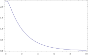
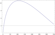
Figure 1: Graph of perturbation $h(t)$ in function of time analyzed in the cases for $a(t)\,=a_{0}e^{H_{0}t}$, $a(t)\,=a_{0}t^{1/2}$ and $a(t)\,=a_{0}t^{2/3}$ respectively, with the initial conditions $h_{0}\,=\,\frac{1}{\sqrt{2n}}$, $\dot{h}\,=\,\sqrt{\frac{n}{2}}$,$\ddot{h}\,=\,\frac{n^{3/2}}{\sqrt{2}}$, $\stackrel{{\scriptstyle...}}{{h}}\,=\,\frac{n^{5/2}}{\sqrt{2}}$, where we adopt $a_{1}\,<\,0$. Stable behavior.

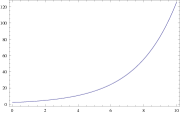
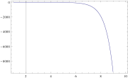
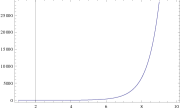
Figure 2: Graph of perturbation $h(t)$ in function of time analyzed in the cases for $a(t)\,=a_{0}e^{H_{0}t}$, $a(t)\,=a_{0}t^{1/2}$ and $a(t)\,=a_{0}t^{2/3}$ respectively, with the initial conditions $h_{0}\,=\,\frac{1}{\sqrt{2n}}$, $\dot{h}\,=\,\sqrt{\frac{n}{2}}$,$\ddot{h}\,=\,\frac{n^{3/2}}{\sqrt{2}}$, $\stackrel{{\scriptstyle...}}{{h}}\,=\,\frac{n^{5/2}}{\sqrt{2}}$, where we adopt $a_{1}\,>\,0$. Unstable behavior.

5 The spectrum of gravitational waves

Before starting to work with the differential equation (33), let us remember some standard notions concerning the spectrum of gravitational waves. For the sake of simplicity we start from the inflationary background case.

Consider the case of gravitational wave on the background of inflationary solution in the theory without quantum corrections. We have

$$\ddot{h}-\frac{\dot{a}\dot{h}}{a}+\Big{\{}\frac{n^{2}}{a^{2}}-\frac{2\,\ddot{a}}{a}\Big{\}}h\,=\,0\,,$$ (52)

where we assume  $a(t)\,=\,a_{0}e^{H_{0}t}$  and also set  $a_{0}\,=\,1$. The vacuum state is well known for this theory (see, e.g., [2]), being

$$h(x,\eta)\,=\,h(\eta)\,e^{\pm i{{\bf n}}\cdot{\bf x}}\,,\qquad h(\eta)\,=\,\frac{e^{\pm i{{\bf n}}\cdot{\bf x}}}{\sqrt{2n}}\,,$$ (53)

where ${{\bf n}}$ is called the wave number vector. In order to study the dynamics of $h(t,{\bf x})$, it is necessary to make a Fourier transform,

$$h_{{{\bf n}}}(t)\,=\,\frac{1}{(2\pi)^{3/2}}\,\int h(t,{\bf x})\,e^{i{{\bf n}}\cdot{\bf x}}\,d^{3}x.$$ (54)

We will need the total square of the amplitude, namely

$$h^{2}(t)\,=\,\int h_{{{\bf n}}}^{2}(t)\,d^{3}n\,.$$ (55)

The above equation can be rewritten in the form

$$h^{2}(t)\,=\,4\pi\int h_{{{\bf n}}}^{2}(t)\,n^{2}\,d\,n\,=\,4\pi\int h^{2}_{{{\bf n}}}(t)\,n^{3}\,d\,\,\mbox{ln}\,\,n\,=\,4\pi\,\int P^{2}_{n}(t)\,d\,\,\mbox{ln}\,\,n\,,$$ (56)

where

$$P^{2}_{n}(t)\,=\,h_{{{\bf n}}}^{2}(t)\,n^{3}\,.$$ (57)

The last quantity is called the “square of the power spectrum”. It shows us how the amplitude of gravitational waves vary in a range of $\,\,\mbox{ln}\,\,n\,$ to $\,\,\mbox{ln}\,(n+dn)$.

Starting from this point one can find the power spectrum for theory with Eq. (52) for the gravitational wave and then apply in our model with Eq. (33). For this end one has to square the value of the gravitational perturbation at a given time and for a given wave number $\,n$. We will vary this $\,n\,$ for a fixed $t$ and simultaneously solve our fourth-order differential equation numerically. After this, we linearize the graph by plotting the relation

$$\,\mbox{ln}\,\,n^{3}\,h_{{{\bf n}}}^{2}(t)\,\times\,\mbox{ln}\,\,n\,.$$ (58)

As a result we obtain the linear proportionality coefficient, which will be denoted as $\,k$ and called spectral index. Then we have, $P^{2}_{n}(t)\,\propto\,n^{k}$ , i.e., it is proportional to the spectral index. It is the power spectrum that will tell us how the amplitude of the perturbations depends on the wavelength.

Let us adopt the initial conditions of quantum origin,

$$h_{0}\,\propto\,\frac{1}{\sqrt{2n}}\,,\qquad\dot{h}\,\propto\,\sqrt{\frac{n}{2}}\,,\qquad\ddot{h}\,\propto\,\frac{n^{3/2}}{\sqrt{2}}\,,\qquad\stackrel{{\scriptstyle...}}{{h}}\,\propto\,\frac{n^{5/2}}{\sqrt{2}}\,.$$ (59)

Then, performing the above procedure for the case of inflation, represented by the equation (52), we found,

$$k\,\approx\,0.01\,\,.$$ (60)

Now, applying the same procedure for our model of equation (33), we find, in the case of exponential expansion without quantum corrections (this means $a_{1}\,=\,a_{2}\,=\,0$),

$$k\,=\,0.00894167\,\approx\,0.01$$ (61)

where we use the units with the Planck mass equal to $1$ in the equation (33) and the Eqs. (28), for perform the numerical analysis. This value is very close to the one which can be found for inflation when we calculate analytically, it should be $\,k\approx 0$, as we can see on (60). Thus the model we are considering returns to the well known inflation case when we take $a_{1}\,=\,a_{2}\,=\,0$. The flat or almost flat spectrum which is found occurs because the stable version of the anomaly-induced inflation develops de Sitter phase with $\,H=const$.

Now we are able to analyze the general quantum case with $a_{1}\,\neq\,0$. Remember that the action for the vacuum is given by (4), where $\,a_{1}$ is most important for the evolution of tensor perturbations. Below we consider three separate cases and present the results of numerical analysis.

5.1 Inflation, or exponential expansion

The variation of the power spectrum with respect to the change of $a_{1}$ (positive and negative) is presented in Table 1.

$a_{1}$	0.0	0.1	0.2	0.3	0.4	0.5	0.6	0.7	0.8	0.9	1.0
$k$	0.01	0.04	0.8	0.12	0.17	0.22	0.29	0.37	0.48	0.61	0.79

Table 1: Getting $k$ through the variation of $a_{1}\,>\,0$ in case of $a(t)\,=\,a_{0}\,e^{H_{0}t}$.

$a_{1}$	0.0	-0.1	-0.2	-0.3	-0.4	-0.5	-0.6	-0.7	-0.8	-0.9	-1.0
$k$	0.01	-0.05	-0.4	-0.06	-0.06	-0.08	-0.09	-0.11	-0.12	-0.13	-0.14

Table 2: Getting $k$ through the variation of $a_{1}\,<\,0$ in case of $a(t)\,=\,a_{0}\,e^{H_{0}t}$.

These two tables show that when the value of $\,a_{1}\,$ is negative and is decreasing, the values of $\,k\,$ also decrease while being negative. That is, as we increase $\,a_{1}$, the amplitude of gravitational waves decrease. In the case of positive $\,a_{1}\,$ an opposite situation happens, namely when we increase its value, the value of $\,k$ is also increasing. This happens because $\,a_{1}\,>\,0\,$ does not represent a stable solution of (33).

These results may be compared with the computation of the spectral index for gravitational waves in the context of the pre-big bang scenario, based on the string effective action at tree level [34]. In this case, the spectral index is positive with the increasing spectrum, while the de Sitter inflation predicts a flat spectrum and power law inflation a negative spectral index, that means the decreasing spectrum.

Now, using the data obtained in [35], [36], [37] and using the software CMBEASY [38] [39] and [40] we can obtain the graph of the spectrum of anisotropy of the cosmic microwave background (CMB) due to gravitational waves for the cases specified above. In these graphs there are two essential quantities, namely the spectral index $\,k\,$ and the content of matter in the universe. The plots for the exponential expansion are shown in Figure 3. In all graphs we use $a_{2}\,=\,0$. However, $k$ value is the same for any $a_{2}$ value.

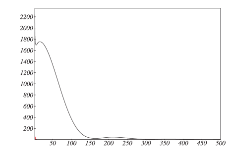
Figure 3: Behavior of the anisotropy spectrum for the three cases with $k\,=\,0.01$. These three solutions have the same $\,k\,$ to $\,a_{1}=0$. That is, they are degenerate.

5.2 Radiation

By performing the same procedure of solving numerically the differential equation (33) and the same linearization as used before, we can test other cases, like radiation where we have $a(t)\,=\,a_{0}\,t^{1/2}$ and matter, where $a(t)\,=\,a_{0}\,t^{2/3}$.

For radiation, we have the results presented in Table 3.

$a_{1}$	0.0	0.1	0.2	0.3	0.4	0.5	0.6	0.7	0.8	0.9	1.0
$k$	0.01	0.05	0.08	0.11	0.13	0.16	0.18	0.21	0.23	0.26	0.29

Table 3: Getting $k$ through the variation of $a_{1}\,>\,0$ in case of $a(t)\,=\,a_{0}\,t^{1/2}$.

$a_{1}$	0.0	-0.1	-0.2	-0.3	-0.4	-0.5	-0.6	-0.7	-0.8	-0.9	-1.0
$k$	0.01	-0.26	-0.27	-0.28	-0.33	-0.30	-0.33	-0.38	-0.38	-0.36	-0.34

Table 4: Getting $k$ through the variation of $a_{1}\,<\,0$ in case of $a(t)\,=\,a_{0}\,t^{1/2}$.

With these values we obtain the graphs shown in Figures 3 and 4, for the anisotropy spectrum, where we take the value  $a_{1}=0$  (Figure 3) and the extreme value  $a_{1}=1$  (Figure 4) from the tables presented above.

5.3 Matter

Finally, we analyze the case for matter-dominated epoch, with $\,a(t)=a_{0}\,t^{2/3}\,$, where we get the values presented in Tables 5 and 6.

$a_{1}$	0.0	0.1	0.2	0.3	0.4	0.5	0.6	0.7	0.8	0.9	1.0
$k$	0.01	0.06	0.09	0.12	0.14	0.17	0.20	0.22	0.25	0.28	0.29

Table 5: Getting $\,k\,$ through the variation of $\,a_{1}>0\,$ in case of $\,a(t)=a_{0}\,t^{2/3}$.

$a_{1}$	0.0	-0.1	-0.2	-0.3	-0.4	-0.5	-0.6	-0.7	-0.8	-0.9	-1.0
$k$	0.01	-0.23	-0.24	-0.24	-0.28	-0.25	-0.28	-0.32	-0.31	-0.29	-0.28

Table 6: Getting $\,k\,$ through the variation of $\,a_{1}<0\,$ in case of $\,a(t)=a_{0}\,t^{2/3}$.

With these values we obtain the graphs for the anisotropy spectrum presented in Figures 3 ($a_{1}=0$) and 4 ($a_{1}=1$).

We can observe that the graphs of the spectrum of CMB anisotropy are nearly identical in the case of radiation and matter (Figure 3), but both are different from the case of inflation. The cases of matter and radiation in Figure 4 are degenerate.

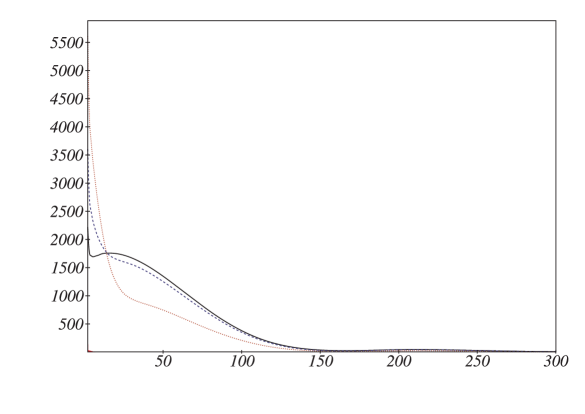
Figure 4: Behavior of the anisotropy spectrum for gravitational waves in de Sitter (black line with $k\,=\,0$), inflation (red line with $k\,=\,0.79$) and Radiation/Matter (blue line with $k\,=\,0.3$ for both). All this is for $a_{1}\,=\,1$.

6 Quantum effects of massive fields and tempered inflation

It was shown in [23, 24] that taking the quantum effects of massive fields into account leads to the tempered form of inflationary solution $\,H_{S}\,$ in (20). The solution which emerges after we derive the corresponding effective equations can be very well approximated by the formula

$$a(t)=e^{\sigma(t)}\,,\qquad\sigma(t)\,=\,H_{0}t-\frac{H_{0}^{2}}{4}\,\tilde{f}\,t^{2}\,,\qquad H(t)\,=\,H_{0}-\frac{H_{0}^{2}}{2}\,\tilde{f}\,t\,,$$ (62)

where $\tilde{f}$ is a small dimensionless parameter, which is at least as small as $10^{-5}$. The plot of this parabolic $\sigma(t)$ this given in Figure 5. This stable phase of inflation is supposed to last until $\,H(t)\,$ becomes comparable to the energy scale of supersymmetry breaking and the transition to the unstable phase of inflation occurs.

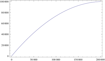
Figure 5: Evolution of $\sigma(t)$.

We can use the solution (62) in our differential equation (33) for the tensor perturbation. Solving this equation numerically and doing linearization as it was explained above, we arrive at the Tables 7 and 8 for the variation of $\,k\,$ with respect to $\,a_{1}\,$ in the case of Modified Starobinsky model of inflation.

$a_{1}$	0.0	0.1	0.2	0.3	0.4	0.5	0.6	0.7	0.8	0.9	1.0
$k$	0.01	0.04	0.08	0.12	0.17	0.22	0.29	0.37	0.48	0.61	0.79

Table 7: Getting $k$ through the variation of $a_{1}\,>\,0$ in case of Eq. (62).

$a_{1}$	0.0	-0.1	-0.2	-0.3	-0.4	-0.5	-0.6	-0.7	-0.8	-0.9	-1.0
$k$	-0.01	-0.02	-0.03	-0.04	-0.05	-0.07	-0.09	-0.11	-0.12	-0.13	-0.14

Table 8: Getting $k$ through the variation of $a_{1}\,<\,0$ in case of Eq. (62).

We can see that the table is almost identical to the one for the case of usual inflation, described in Table 1. This is because the parameter $\tilde{f}$ is small $\,10^{-5}\,$ and the desacceleration of inflation happens slower compared to the typical scale of tensor perturbations. If we consider this parameter being increased, the two results begin to diverge from each other. The values of $\,k\,$ increase as the value of $\,\tilde{f}\,$ increase too.

7 Conclusions

The classical action of gravity which is necessary to guarantee the renormalizable theory of matter fields on classical metric background goes beyond the conventional Einstein-Hilbert term, for it includes also the cosmological constant term and higher derivative terms. The presence of higher derivatives is usually associated to the problem of higher derivative unphysical ghosts, but this issue does not represent a real problem for the theory when gravity is only an external background and there is no unitarity condition for the gravitational $S$-matrix. In the case of external gravity the necessary consistency conditions should be the existence of physically acceptable solutions and their robustness. The last criteria means that these solutions must be stable, at least, with respect to the small perturbations of the metric variables. In case of gravity the higher derivative terms can be especially dangerous for the stability of classical cosmological solutions, such as matter and radiation - dominated Universes and the Universe dominated by the cosmological constant term. The results found here shows that the detection of the gravitational wave contribution to the spectrum of anisotropy of the cosmic microwave background radiation (which may be possible with the Planck satellite) could lead to important bounds on the possible quantum effects analysed in this paper.

On the top of the classical vacuum terms there are also quantum corrections to it. One of the best available forms of such corrections is the anomaly-induced effective action of vacuum, which is especially efficient as an approximation to the present-day Universe, when all quantum fields except the photon have already decoupled from gravity and the quantum contribution of photon fits perfectly to the anomaly-induced approach.

We have used the anomaly-induced action of gravity to explore the behavior of tensor perturbations and especially to verify the stability of classical cosmological solutions with respect to such perturbations. The consideration was based on explicit derivation of gravitational wave equations in the theory with anomaly-induced quantum corrections and on the use of both analytical and numerical methods to perform the detailed analysis of these equations. The main conclusion of our work is that the stability conditions are essentially related to the sign of the Weyl-squared term in the classical action of vacuum and do not manifest any essential dependence on the quantum contributions. The qualitative explanation of this result is that the anomaly-induced action has a structure which prevents it to give essential contributions to the linear equation for tensor perturbations. Let us note that the situation may be very different for the density perturbations, where the sign of the $R^{2}$-term may be most relevant and for the non-linear perturbations, where the mentioned qualitative arguments simply do not hold.

Appendix A Roots of the quartic polynomial equation

Here we present the analysis of the fourth-order polynomial which was used in Section 4. Consider the polynomial,

$$\lambda^{4}+d_{3}\lambda^{3}+d_{2}\lambda^{2}+d_{1}\lambda^{1}+d_{0}\,=\,0\,.$$ (63)

Let us follow the classical Cardano method. To eliminate the cubic term make the substitution $\lambda\,=\,x-\frac{d_{3}}{4}$. We get

$$x^{4}+px^{2}+qx+r\,=\,0\,,$$ (64)

where

$$p\, = \,\frac{d_{3}^{2}}{8}-\frac{d_{3}^{2}}{2}+d_{2}\,,$$ (65)

$$q\, = \,\frac{d_{3}^{2}}{8}-\frac{d_{3}d_{2}}{2}+d_{1}\,,$$ (66)

$$r\, = \,-\frac{3d_{3}^{4}}{256}+\frac{d_{2}d_{3}^{2}}{16}-\frac{d_{2}d_{1}}{4}+d_{0}\,.$$ (67)

Now we rewrite (64) as

$$x^{4}+px^{2}\,=\,-qx-r$$

by completing the square and adding the $y$ term. We obtain

$$y^{3}+\alpha y^{2}+\beta y+\gamma\,=\,0\,,$$ (68)

where

$$\alpha\, = \,\frac{20}{8}\,p\,,$$ (69)

$$\beta\, = \,2p^{2}-r\,,$$ (70)

$$\gamma\, = \,\frac{1}{8}(q^{2}-4p^{3}+4pr)\,.$$ (71)

In order to eliminate the second degree term in (68), make one more substitution $y\,=\,z+m$, where $m\,=\,-\alpha/2$.

$$z^{3}+\xi_{1}z+\xi_{2}\,=\,0\,,$$ (72)

where

$$\xi_{1}\, = \,-\frac{\alpha}{3}+\beta\,,$$ (73)

$$\xi_{2}\, = \,\frac{2\alpha^{3}}{27}+\frac{3\gamma-\beta\gamma}{3}\,.$$ (74)

For the equation (72) one can already apply the Cardano formula and find

$$\Delta\,=\,\xi_{1}+\,\frac{4}{27}\,\xi^{3}\,=\,4\Biggl{[}\Bigl{(}\frac{\xi_{1}}{2}\Bigl{)}^{2}+\Bigl{(}\frac{\xi_{2}}{3}\Bigl{)}^{3}\Biggl{]}\,.$$ (75)

The solution is

$$z\,=\,\sqrt[3]{-\frac{\xi_{1}}{2}+\sqrt{\Bigl{(}\frac{\xi_{1}}{2}\Bigl{)}^{2}+\Bigl{(}\frac{\xi_{2}}{3}\Bigl{)}^{3}}}+\sqrt[3]{-\frac{\xi_{1}}{2}-\sqrt{\Bigl{(}\frac{\xi_{1}}{2}\Bigl{)}^{2}+\Bigl{(}\frac{\xi_{2}}{3}\Bigl{)}^{3}}}\,,$$ (76)

or

$$z\,=\,\sqrt[3]{-\frac{\xi_{1}}{2}+\frac{1}{2}\sqrt{\Delta}}+\sqrt[3]{-\frac{\xi_{1}}{2}-\frac{1}{2}\sqrt{\Delta}}\,.$$ (77)

As far as we know the values of $z$, $m$, $\alpha$ and $p$, it is possible to find the roots $\lambda$.

References

- [1] R. Utiyama, B.S. DeWitt, J. Math. Phys. 3(1962) 608.
- [2] N.D. Birell and P.C.W. Davies, Quantum Fields in Curved Space (Cambridge University Press, Cambridge, 1982).
- [3] I.L. Buchbinder, S.D. Odintsov and I.L. Shapiro, Effective Action in Quantum Gravity (IOP Publishing, Bristol, 1992).
- [4] I. L. Shapiro, Class. Quant. Grav. 25, 103001 (2008) [arXiv:0801.0216 [gr-qc]].
- [5] K. S. Stelle, Gen. Rel. Grav. 9, 353 (1978).
- [6] M.J. Duff, Nucl. Phys. B125 (1977) 334; S. Deser, M.J. Duff and C. Isham, Nucl. Phys. B111 (1976) 45.
- [7] A.A. Starobinski, Phys.Lett. 91B (1980) 99; Nonsingular Model of the Universe with the Quantum-Gravitational De Sitter Stage and its Observational Consequences, Proceedings of the second seminar ”Quantum Gravity”, pp. 58-72 (Moscow, 1982); JETP Lett. 30 (1979) 719; 34 (1981) 460; Let.Astr.Journ. (in Russian), 9 (1983) 579.
- [8] S.M. Christensen and S.A. Fulling, Phys. Rev. D15 (1977) 2088.
- [9] R. Balbinot, A. Fabbri and I.L. Shapiro, Phys. Rev. Lett. 83 (1999) 1494; Nucl. Phys. B559 (1999) 301.
- [10] P.R. Anderson, E. Mottola, R. Vaulin, Stress Tensor from the Trace Anomaly in Reissner-Nordstrom Spacetimes. Phys.Rev. D76 (2007) 124028; gr-qc/0707.3751.
- [11] A.A. Starobinski, Let.Astr.Journ. (in Russian), 9 (1983) 579.
- [12] S.W. Hawking, T. Hertog and H.S. Real, Phys.Rev. D63 (2001) 083504.
- [13] J. C. Fabris, A. M. Pelinson and I. L. Shapiro, Nucl. Phys. B 597, 539 (2001) [Erratum-ibid. B 602, 644 (2001)] [arXiv:hep-th/0009197].
- [14] E.V. Gorbar, I.L. Shapiro, JHEP 02 (2003) 021; JHEP 06 (2003) 004; JHEP 02 (2004) 060.
- [15] T.W.B. Kibble and S. Randjbar-Daemi, J. Phys. A: Math. Gen. 13 ( 1980) 141; S. Randjbar-Daemi, J. Phys.A A14 (1981) L229.
- [16] B. Biran, R. Brout and E. Gunzig, On The Stability And Instability Of Minkowski Space In The Presence Of Quantized Matter Fields. Phys.Lett. B125 (1983) 399.
- [17] D. Gross, M. Perry and L. Yaffe, Phys. Rev. D25 (1982) 330.
- [18] Paul R. Anderson, Carmen Molina-Paris, Emil Mottola, Phys. Rev. D67 (2003) 024026 e-Print: gr-qc/0209075
- [19] G. Perez-Nadal, A. Roura and E. Verdaguer, Phys. Rev. D77 (2008) 124033, arXiv:0712.2282 [gr-qc]; Class. Quantum Grav. 25 (2008) 154013; B.L. Hu, A. Roura and E. Verdaguer, Int. J. Theor. Phys. 43 (2004) 749; A. Roura and E. Verdaguer, Phys.Rev. D78 (2008) 064010, arXiv:0709.1940 [gr-qc].
- [20] C.P. Burgess, R. Holman, L. Leblond and S. Shandera, JCAP 1010 (2010) 017; e-Print: arXiv:1005.3551 [hep-th].
- [21] M. V. Fischetti, J. B. Hartle and B. L. Hu, Phys. Rev. D 20, 1757 (1979).
- [22] V.F. Mukhanov and G.V. Chibisov, JETP Lett. 33 (1981) 532; JETP (1982) 258.
- [23] I.L. Shapiro, J. Solà, Phys. Lett. B530 (2002) 10; I.L. Shapiro, Int. Journ. Mod. Phys. 11D (2002) 1159.
- [24] A. M. Pelinson, I. L. Shapiro and F. I. Takakura, Nucl. Phys. B 648 (2003) 417.
- [25] R.J. Riegert, Phys.Lett. 134B (1984) 56.
- [26] E.S. Fradkin and A.A. Tseytlin, Phys.Lett. 134B (1984) 187.
- [27] S. G. Mamaev and V. M. Mostepanenko, Sov. Phys. JETP 51 (1980) 9 [Zh. Eksp. Teor. Fiz. 78 (1980) 20].
- [28] A. Vilenkin, Phys. Rev. D32 (1985) 2511.
- [29] I.L. Shapiro and A.G. Jacksenaev, Phys. Lett. 324B (1994) 284.
-
[30]
P. O. Mazur and E. Mottola,
Phys. Rev. D 64, 104022 (2001);
E.Mottola and R. Vaulin, Phys. Rev. D74 (2006) 064004; e-Print: gr-qc/0604051. - [31] A.M. Pelinson and I.L. Shapiro, Phys. Lett. B694 (2011) 467, arXiv:1005.1313; Int. J. Mod. Phys. A26 (2011) 3759.
- [32] M. Gasperini, Phys. Rev. D 56, 4815 (1997)
-
[33]
S. Wolfram, The MATHEMATICA Book, Version 6;
www.wolfram.com/mathematica/. - [34] M. Gasperini and G. Veneziano, Phys. Rept. 373 (2003) 1.
- [35] D. Larson et al., Astrophys. J. Suppl. 192 (2011) 16 [arXiv:1001.4635 [astro-ph.CO]].
- [36] E. Komatsu et al. [WMAP Collaboration], Astrophys. J. Suppl. 192 (2011) 18 [arXiv:1001.4538 [astro-ph.CO]].
- [37] J. Dunkley et al. [WMAP Collaboration], Astrophys. J. Suppl. 180 (2009) 306 [arXiv:0803.0586 [astro-ph]].
- [38] http://www.thphys.uni-heidelberg.de/robbers/cmbeasy/.
- [39] M. Doran, JCAP 0510 (2005) 011 [arXiv:astro-ph/0302138].
- [40] M. Doran and C. M. Mueller, JCAP 0409 (2004) 003 [arXiv:astro-ph/0311311].