Explicit Integration of Extremely-Stiff Reaction Networks: Partial Equilibrium Methods

Abstract

In two preceding papers [1, 2] we have shown that, when reaction networks are well-removed from equilibrium, explicit asymptotic and quasi-steady-state approximations can give algebraically-stabilized integration schemes that rival standard implicit methods in accuracy and speed for extremely stiff systems. However, we also showed that these explicit methods remain accurate but are no longer competitive in speed as the network approaches equilibrium. In this paper we analyze this failure and show that it is associated with the presence of fast equilibration timescales that neither asymptotic nor quasi-steady-state approximations are able to remove efficiently from the numerical integration. Based on this understanding, we develop a partial equilibrium method to deal effectively with the approach to equilibrium and show that explicit asymptotic methods, combined with the new partial equilibrium methods, give an integration scheme that plausibly can deal with the stiffest networks, even in the approach to equilibrium, with accuracy and speed competitive with that of implicit methods. Thus we demonstrate that such explicit methods may offer alternatives to implicit integration of even extremely stiff systems, and that these methods may permit integration of much larger networks than have been possible before in a number of fields.

Keywords: ordinary differential equations, reaction networks, stiffness, reactive flows, nucleosynthesis, combustion

1 Introduction

Problems from many fields of science and technology require the solution of large coupled reaction networks describing the flow of population between various sources and sinks. Some important examples include reaction networks in combustion chemistry [3], geochemical cycling of elements [4], and thermonuclear reaction networks in astrophysics [5, 6]. The systems of differential equations that are commonly used to model these reaction networks usually exhibit stiffness, which we may think of loosely as arising from multiple timescales in the problem that differ by many orders of magnitude [3, 7, 8, 9]. The most straightforward way to solve such a system might appear to be an explicit numerical integration scheme (for an explicit method, advancing a timestep requires only information known from previous timesteps). However, the textbooks routinely state [3, 8, 9] that such systems cannot be integrated efficiently using explicit forward finite-difference methods because of stability issues: for an explicit algorithm, the maximum stable timestep in a stiff system is typically set by the fastest timescales, even if those timescales are not of central interest. The traditional solution of the stiffness problem is to replace explicit integration with implicit integration (integration methods that require the values for derivatives at timesteps not yet evaluated).

The astrophysical CNO cycle for conversion of hydrogen to helium (Fig. 1) is an instructive example of the stiffness issue. In the CNO cycle the fastest rates typically are $\beta$-decays with half-lives of order 100 seconds, but tracking main-sequence hydrogen burning may require integration of the hydrogen-burning network for as long as billions of years ($\sim 10^{16}$ seconds). With explicit forward differencing the largest stable integration timestep is set by the fastest rates and will be of order $10^{2}$ seconds, so $\sim 10^{14}$ explicit integration steps could be required, even for the idealized case of constant temperature and density. Conversely, this same numerical integration requires at most a few hundred steps using implicit methods. For this reason, it is generally thought that explicit methods are not viable for extremely stiff networks. To quote Numerical Recipes [9], “For stiff problems we must use an implicit method if we want to avoid having tiny stepsizes.”

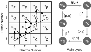
Figure 1: The CNO cycle. On the left side the main branch of the cycle is illustrated with solid arrows and a side branch is illustrated with dashed arrows. On the right side, the main branch of the CNO cycle is illustrated in more detail ($p$ stands for ¹H and $\alpha$ for ⁴He).

Although implicit methods typically are stable for stiff systems, they require substantial additional computational overhead relative to explicit methods. For large coupled sets of equations, this normally takes the form of iterative solutions that require the inversion of large matrices at each step. The required matrix inversions dictate that, except where simplifications based on matrix structure can be exploited (for example, sparse-matrix methods), implicit algorithms may scale as poorly as quadratically or cubically with the size of the network. Thus, implicit methods can be expensive to implement for large networks, particularly those that are coupled in real time to a broader problem such as hydrodynamical evolution.

Despite the generally negative view of explicit methods for stiff systems sketched in the preceding paragraphs, they would be attractive options for complex networks if they could take larger timesteps because of their overall simplicity and highly-favorable linear scaling with network size relative to implicit methods. To increase the integration step size for explicit methods obviously requires overcoming formidable numerical stability problems that are associated with the stiffness. In principle, this might be accomplished by using approximate analytical solutions to reduce the stiffness of the equation set to be solved, thereby improving the overall stability of the network. In the first two papers of this series [1, 2], we have shown in a variety of examples that this can be accomplished for systems that are not near equilibrium by using asymptotic and quasi-steady-state approximations to stabilize the numerical integration. However, as we shall now discuss, the nature of stiffness is different for networks that are near equilibrium. This implies that the modifications required to stabilize standard explicit methods when stiffness is encountered far from equilibrium must be altered when that same network approaches equilibrium.

2 Varieties of Stiffness

For the large and very stiff networks that are our primary interest here there are several fundamentally different sources of stiffness instability. Most textbook discussions of stiffness concentrate on an instability associated with small quantities that strictly should be non-negative being driven negative by an overly-ambitious numerical integration step. However, there are other guises that stiffness can take, as we now discuss. The equations that we must integrate take the general form

$$\frac{dy_{i}}{dt} = F^{+}_{i}-F^{-}_{i}$$ (1)

$$= (f^{+}_{1}+f^{+}_{2}+\ldots)_{i}-(f^{-}_{1}+f^{-}_{2}+\ldots)_{i}$$

$$= (f^{+}_{1}-f^{-}_{1})_{i}+(f^{+}_{2}-f^{-}_{2})_{i}+\ldots=\sum_{j}(f^{+}_{j}-f^{-}_{j})_{i},$$

where the $y_{i}(i=1\dots N)$ describe the dependent variables (abundance in our examples), $t$ is the independent variable (time in our examples), the fluxes between species $i$ and $j$ are denoted by $(f^{\pm}_{j})_{i}$, and the sum for each variable $i$ is over all variables $j$ coupled to $i$ by a non-zero flux $(f^{\pm}_{j})_{i}$. For an $N$-species network there will be $N$ such equations in the populations $y_{i}$, generally coupled to each other because of the dependence of the fluxes on the different $y_{j}$.

Because our discussion is intended to be quite general, we shall most often formulate the equations (1) in terms of generic population variables $y_{i}$ that are assumed to be proportional to the number density of species $i$. Where we give specific results for astrophysical networks, we shall use population variables most common for that field, such as the mass fraction $X_{i}$ and the (molar) abundance $Y_{i}$, with

$$X_{i}=\frac{n_{i}A_{i}}{\rho N_{\mbox{\scriptsize A}}}\qquad Y_{i}\equiv\frac{X_{i}}{A_{i}}=\frac{n_{i}}{\rho N_{\mbox{\scriptsize A}}}$$ (2)

where $N_{\mbox{\scriptsize A}}$ is Avogadro’s number, $\rho$ is the total mass density, $A_{i}$ is the atomic mass number and $n_{i}$ the number density for the species $i$, and by definition the mass fractions sum to unity if nucleon number is conserved: $\sum X_{i}=1$.

In Eq. (1) the total flux has been decomposed into a component $F^{+}_{i}$ that increases the population $y_{i}$ and a component $F^{-}_{i}$ that depletes the population $y_{i}$, and in the third line this has been decomposed further into individual groups of terms $f^{+}_{j}-f^{-}_{j}$. In the approach to equilibrium a species population entails a delicate balance between a total flux $F^{+}_{i}$ populating the species and a total flux $F^{-}_{i}$ depleting it. Near equilibrium the difference $F_{i}=F^{+}_{i}-F^{-}_{i}$ can be orders of magnitude smaller than $F^{+}_{i}$ or $F^{-}_{i}$ and small numerical errors in $F^{+}_{i}$ or $F^{-}_{i}$ can produce large errors in the difference $F_{i}$. Because of the population coupling in complex networks, this error propagates and compromises the accuracy of the network unless the timestep is short enough that the difference $F_{i}$ is computed accurately for each population in the network. But this restriction means that the maximum timestep is set by the largest fluxes (that is, the largest stable timestep is determined by the inverses of the highest rates); this lands us back in the explicit integration conundrum that the maximum stable timestep is set by the fastest transitions, even if the primary interest is in quantities varying on a much longer timescale.

Thus, in the approach to equilibrium the problem with explicit integration is not negative populations directly, but an unacceptable loss of accuracy that may occur even before any populations become negative. This is still a stiffness issue because it involves stability in systems with disparate timescales. In this case the contrasting timescales are the very rapid reactions driving the system to equilibrium relative to the very slow timescale associated with equilibrium itself. Thus any system nearing equilibrium can be expected to exhibit this form of stiffness instability. As we now address, this distinction among sources of stiffness is critical because these stiffness instabilities have fundamentally different causes and thus fundamentally different solutions. Furthermore, we shall find that the second class of instabilities can be divided into two subclasses requiring different stabilizing approximations. The approximations that we shall introduce in all these cases take care naturally of the first class of stiffness instabilities because they will prevent the occurrence of negative probabilities.

3 Curing Stiffness in the Approach to Equilibrium

We shall take equilibration to mean a situation where populations in the network are being strongly influenced by canceling terms on the right sides of the differential equations (1). In terms of the coupled set of differential equations describing the network, we may distinguish two qualitatively different conditions:

1. An equilibration acting at the level of individual differential equations that we shall call macroscopic equilibration.

2. An equilibration acting at the level of subsets of terms within a given differential equation that we shall term microscopic equilibration.

Let us consider each of these cases in turn.

3.1 Macroscopic Equilibration

The differential equations that we must solve take the general form given in Eq. (1), $dy_{i}/dt=F^{+}_{i}-F^{-}_{i}$. One class of approximate solutions depends upon assuming that $F^{+}_{i}-F^{-}_{i}\rightarrow 0$ (asymptotic approximations) or $F^{+}_{i}-F^{-}_{i}\rightarrow$ constant (quasi-steady-state approximations). We shall term this macroscopic equilibration, since these conditions involve the entire right side of a differential equation in Eq. (1) tending to zero or a finite constant. In the first two papers of this series [1, 2] we employed asymptotic and quasi-steady-state approximations that removed entire differential equations from the numerical integration for a network timestep by replacing them with algebraic approximate solutions for that timestep. These approximations integrate the full original set of differential equations, but they reduce the number of equations integrated numerically. This removal of equations from the numerical integration reduces the stiffness because it generally decreases the range of timescales in the numerical integration.

3.2 Microscopic Equilibration

In Eq. (1), $F^{+}_{i}$ and $F^{-}_{i}$ for a given species $i$ each consist of a number of terms depending on the various populations in the network,

$$\frac{dy_{i}}{dt} = F^{+}_{i}-F^{-}_{i}=\sum_{j}(f^{+}_{j}-f^{-}_{j})_{i}.$$ (3)

At the more microscopic level, groups of individual terms on the right side of Eq. (1) in the sum over $j$ may come approximately into equilibrium (so that the sum of their fluxes is approximately zero), even if the macroscopic conditions for equilibration are not satisfied and asymptotic or quasi-steady-state approximations are not well justified for the species $i$. The simplest possibility is that forward–reverse reaction pairs such as $A+B\rightleftharpoons C$, which will contribute flux terms with opposite signs on the right sides of differential equations in which they participate, come approximately into equilibrium. As we shall demonstrate, this introduces new (often fast) timescales into the problem that are at best only partially removed by asymptotic and quasi-steady-state (QSS) approximations. The new sources of stiffness associated with these microscopic equilibration effects explain why asymptotic and QSS approximations remain accurate but their timestepping becomes very inefficient in the approach to equilibrium.

As we elaborate in the remainder of this paper, this new source of stiffness associated with close approach to microscopic equilibration requires a new algebraic approximation that removes groups of such terms from the numerical integration by replacing their sum of fluxes with zero. Such an approximation will not generally reduce the number of equations to be integrated numerically in a network timestep, but can (dramatically, as we shall see) reduce the stiffness of those equations by systematically removing terms with fast rates from the equations. This reduces the disparity between the fastest and slowest timescales in the system. Thus shall we convert the approach to equilibrium in an explicit integration from a liability into an asset. As part of this elaboration we shall also reach two important general conclusions: (1) Approximations based on microscopic equilibration are much more efficient at removing stiffness than those based on macroscopic equilibration, because they more precisely target the sources of stiffness in the network. (2) Macroscopic and microscopic approximations can complement each other in removing stiffness from the equations to be integrated numerically and thus the two together are more powerful than either used alone.

4 Methods for Partial Equilibrium

Let us begin to develop some methods to deal effectively with explicit integration in the approach to equilibrium. In doing so we draw substantially on the work of David Mott [10], but we will extend these methods and obtain much more favorable results for extremely stiff networks than those obtained in the original work of Mott and collaborators.

The basic idea of partial equilibrium (PE) methods is to inspect the source terms $f^{+}_{i}$ and $f^{-}_{i}$ associated with individual reaction pairs in the network for approach to equilibrium (instead of the composite flux terms $F^{+}_{i}$ and $F^{-}_{i}$ that are the basis for asymptotic and quasi-steady-state approximations). Once a fast reaction pair nears equilibrium, its source terms are removed from the direct numerical integration in the ordinary differential equations and its effect is incorporated through an algebraic constraint implied by the equilibrium condition. Those reactions not in equilibrium still contribute to the net fluxes for the numerical integrator, but once the fast reactions associated with an equilibrating reaction pair are decoupled from the numerical integration the remaining system typically becomes much less stiff. To illustrate, consider a representative 2-body reaction,

$$a+b\rightleftharpoons c+d.$$ (4)

The source term for this reaction pair can be expressed in the general form

$$f_{{ab}{\rightleftharpoons}{cd}}=\pm(f_{a+b\rightarrow c+d}-f_{c+d\rightarrow a+b})=\pm(k_{\mbox{\scriptsize f}}y_{a}y_{b}-k_{\mbox{\scriptsize r}}y_{c}y_{d}),$$ (5)

where the $y_{i}$ denote population variables for the species $i$ and the $k$s are rate parameters. This source term will contribute to the right side of the differential equations describing the change in population for all four species $a,b,c,d$:

$$\frac{dy_{a}}{dt}\hskip 0.0pt = \hskip 0.0ptf_{{ab}{\rightleftharpoons}{cd}}+{\rm other\ terms\ changing\ }y_{a}$$ (6)

$$\frac{dy_{b}}{dt}\hskip 0.0pt = \hskip 0.0ptf_{{ab}{\rightleftharpoons}{cd}}+{\rm other\ terms\ changing\ }y_{b}$$ (7)

$$\frac{dy_{c}}{dt}\hskip 0.0pt = \hskip 0.0pt-f_{{ab}{\rightleftharpoons}{cd}}+{\rm other\ terms\ changing\ }y_{c}$$ (8)

$$\frac{dy_{d}}{dt}\hskip 0.0pt = \hskip 0.0pt-f_{{ab}{\rightleftharpoons}{cd}}+{\rm other\ terms\ changing\ }y_{d}$$ (9)

Thus removing or reducing the stiffness associated with this single reaction pair influences a whole set of populations and associated reactions, and so can reduce the overall stiffness of the system. Strictly, the reaction pair of Eq. (4) is in equilibrium if $f_{{ab}{\rightleftharpoons}{cd}}=0$. Of greater interest will be partially-equilibrated systems, where some reactions maintain $f\sim 0$ as the system evolves but others have $f\neq 0$ (and the members of these two sets may change over time). Our goal will be to develop methods to integrate such systems using asymptotic or quasi-steady-state algorithms, but for modified equations of reduced stiffness in which the flux sums for the $f\sim 0$ reactions have been replaced by equilibrium constraints.

From Eqs. (4)–(9) the single reaction pair $a+b\rightleftharpoons c+d$ appears to have four characteristic timescales associated with the rate of change for the four populations $y_{a}$, $y_{b}$, $y_{c}$, and $y_{d}$, respectively. For $a+b\rightleftharpoons c+d$ considered in isolation, the differential equation governing the abundance of species $a$ is

$$\frac{dy_{a}}{dt}=F^{+}_{a}-F^{-}_{a}=k_{\mbox{\scriptsize r}}y_{c}y_{d}-k_{\mbox{\scriptsize f}}y_{a}y_{b}=F^{+}_{a}-\frac{y_{a}}{\tau_{a}},$$

where $\tau_{a}\equiv 1/(k_{\mbox{\scriptsize f}}y_{b})$. If we assume the abundances of $c$ and $d$ and the rate parameters to remain approximately constant in a timestep, the timescale $\tau_{a}$ characterizes the rate of change of the species $a$. Likewise, for the other three components of the reaction pair we may write similar differential equations and define similar timescales,

$$\tau_{a}=\frac{1}{k_{\mbox{\scriptsize f}}y_{b}}\quad\tau_{b}=\frac{1}{k_{\mbox{\scriptsize f}}y_{a}}\quad\tau_{c}=\frac{1}{k_{\mbox{\scriptsize r}}y_{d}}\quad\tau_{d}=\frac{1}{k_{\mbox{\scriptsize r}}y_{c}}.$$

Our first task is to construct a single timescale that characterizes equilibration of a reaction pair such as $a+b\rightleftharpoons c+d$, considered in isolation. To do so we introduce the idea of conserved scalars [10].

4.1 Conserved Scalars and Progress Variables

As a simple initial illustration, consider the reaction pair $a\rightleftharpoons 2b$, which has a source term

$$f_{{a}{\rightleftharpoons}{2b}}=k_{\mbox{\scriptsize f}}y_{a}-k_{\mbox{\scriptsize r}}y_{b}^{2}.$$ (10)

If no other reactions altered the populations $y_{a}$ and $y_{b}$,

$$\frac{dy_{a}}{dt}=-f_{{a}{\rightleftharpoons}{2b}}\qquad\frac{dy_{b}}{dt}=2f_{{a}{\rightleftharpoons}{2b}}.$$ (11)

Thus $2dy_{a}/dt+dy_{b}/dt=0$ and $2y_{a}+y_{b}={\rm constant}$. The quantity $2y_{a}+y_{b}$ is an example of a conserved scalar. It is conserved by virtue of the structure of $a\rightleftharpoons 2b$, not by any particular dynamical assumptions; thus conservation of this quantity is independent of whether the reaction is near equilibrium or not. It is convenient to introduce new variables that are the difference between the initial values of $y_{i}$ and their current values

$$\delta y_{a}\equiv y_{a}-y_{a}^{0}\qquad\delta y_{b}=y_{b}-y_{b}^{0}.$$

The initial values $y_{a}^{0}$ and $y_{b}^{0}$ are constants so the differential equations (11) can then be written as

$$\frac{d\delta y_{a}}{dt}=-f_{{a}{\rightleftharpoons}{2b}}\qquad\frac{d\delta y_{b}}{dt}=2f_{{a}{\rightleftharpoons}{2b}}.$$ (12)

This suggests defining a progress variable $\lambda$ for the reaction characterized by $f_{{a}{\rightleftharpoons}{2b}}$ which satisfies

$$\frac{d\lambda}{dt}=f_{{a}{\rightleftharpoons}{2b}}\qquad\lambda_{0}\equiv\lambda(t=0)=0.$$ (13)

By comparing Eq. (13) with Eq. (12) we have $\lambda=-\delta y_{a}=\mbox{$\small\frac{1}{2}$}\delta y_{b}$, so that

$$y_{a}=\delta y_{a}+y_{a}^{0}=-\lambda+y_{a}^{0}\qquad y_{b}=\delta y_{b}+y_{b}^{0}=2\lambda+y_{b}^{0}.$$ (14)

Thus Eqs. (10) and (11) may be rewritten in terms of the single variable $\lambda$ and the solution of two differential equations for two unknowns is reduced to the solution of Eq. (13) for a single unknown $\lambda$ [which may then be used to compute $y_{a}$ and $y_{b}$ through Eq. (14)].

Let’s now apply these ideas to the general 2-body reaction $a+b\rightleftharpoons c+d$ of Eq. (4). Assuming conservation of particle number, it is clear that the following constraints apply to this reaction

$$y_{a}-y_{b}=c_{1}\qquad y_{a}+y_{c}=c_{2}\qquad y_{a}+y_{d}=c_{3},$$ (15)

where the $c_{i}$ are constants. Losing one $a$ by this reaction requires the simultaneous loss of one $b$, so their difference must be constant, and every loss of one $a$ produces one $c$ and one $d$, which explains the second and third equations. These constraints follow entirely from the structure of the reaction and are independent of dynamics. The constants can be evaluated by substituting the initial abundances into Eq. (15),

$$c_{1}=y_{a}^{0}-y_{b}^{0}\qquad c_{2}=y_{a}^{0}+y_{c}^{0}\qquad c_{3}=y_{a}^{0}+y_{d}^{0}.$$

The differential equation for $y_{a}$ is

$$\frac{dy_{a}}{dt}=-k_{\mbox{\scriptsize f}}y_{a}y_{b}+k_{\mbox{\scriptsize r}}y_{c}y_{d},$$ (16)

which can be rewritten using Eq. (15) as

$$\frac{dy_{a}}{dt}=ay_{a}^{2}+by_{a}+c,$$ (17)

where

$$a=k_{\mbox{\scriptsize r}}-k_{\mbox{\scriptsize f}}\qquad b=-k_{\mbox{\scriptsize r}}(c_{2}+c_{3})+k_{\mbox{\scriptsize f}}c_{1}\qquad c=k_{\mbox{\scriptsize r}}c_{2}c_{3}.$$

As we demonstrate below, the approach to equilibrium for any 2-body reaction pair can be described by a differential equation of this form, and the approach to equilibrium for any 3-body reaction pair can be approximated by a differential equation of this form. If $a=0$ the solution of this differential equation gives the quasi-steady-state (QSS) solution, which we have already examined in the second paper of this series [2]. For the general case $a\neq 0$, let us define a quantity

$$q\equiv 4ac-b^{2}\leq 0.$$ (18)

The case $q=0$ is the trivial solution where all abundances are zero, so we are interested in solving Eq. (17) for negative values of $q$. The general solution for $a\neq 0$ and $q<0$ is [10, 11]

$$y_{a}(t)=-\frac{1}{2a}\left(b+\sqrt{-q}\,\frac{1+\phi\exp(-\sqrt{-q}\,t)}{1-\phi\exp(-\sqrt{-q}\,t)},\right)$$ (19)

where

$$\phi=\frac{2ay_{0}+b+\sqrt{-q}}{2ay_{0}+b-\sqrt{-q}}.$$ (20)

The equilibrium solution corresponds to the limit $t\rightarrow\infty$ of Eq. (19):

$$\bar{y}_{a}\equiv y^{{\rm\scriptstyle eq}}_{a}=-\frac{1}{2a}(b+\sqrt{-q}).$$ (21)

By analogy with the earlier discussion we define a progress variable

$$\lambda(t)=-y_{a}(t)+y_{a}^{0}.$$ (22)

Once $y_{a}$ has been determined the constraints (15) may be used to determine the other abundances:

$$y_{b}(t)=y_{a}(t)-c_{1}\quad y_{c}(t)=c_{2}-y_{a}(t)\quad y_{d}(t)=c_{3}-y_{a}(t).$$

The approach of the reaction $a+b\rightleftharpoons c+d$ to equilibrium is thus governed by a single differential equation (17), which may be expressed in terms of either a single one of the abundances $y_{i}$, or the progress variable $\lambda$ defined in Eq. (22). The general solution of this differential equation is given by Eq. (19), from which the rate at which the reaction $a+b\rightleftharpoons c+d$ evolves toward the equilibrium solution (21) is determined by a single timescale

$$\tau=\frac{1}{\sqrt{-q}}.$$ (23)

These equilibrium timescales are illustrated in Fig. 2.

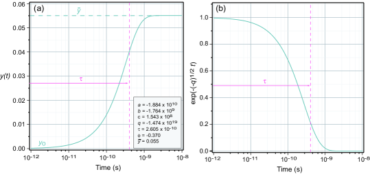
Figure 2: (a) Time evolution of the solution (19) assuming $a$, $b$, and $c$ to remain constant. The characteristic timescale for approach to equilibrium defined by Eq. (23) is labeled $\tau$ and the equilibrium value of $y(t)$ defined by Eq. (21) is denoted by $\bar{y}$. To illustrate we have assumed the initial value $y_{0}=0$. For times considerably larger than $\tau$ the general solution (19) saturates at the equilibrium solution (21). (b) Behavior of the exponential factor in Eq. (19).

We may then estimate whether a reaction is near equilibrium at time $t$ by requiring

$$\frac{|y_{i}(t)-\bar{y}_{i}|}{\bar{y}_{i}}<\epsilon_{i}$$ (24)

for each species $i$ involved in the reaction, where $y_{i}(t)$ is the actual abundance, $\bar{y}_{i}$ is the equilibrium abundance computed from Eq. (21), and the user-specified tolerance $\epsilon_{i}$ can depend on $i$ but will be taken to be the same for all species in the simplest implementation. Alternatively, the equilibrium timescale (23) in comparison with the current numerical timestep may be used as a measure of whether a reaction is near equilibrium. If $\tau$ is much less than the timestep, it is likely that equilibrium can be established and maintained in successive timesteps, even if it is being continually disturbed by other non-equilibrated processes.

4.2 Reaction Vectors

In a large reaction network there could be thousands of reactions to be examined for their equilibrium status at each timestep, so implementation of a partial equilibrium approximation requires a substantial amount of bookkeeping. Our task will be facilitated by systematic ways to catalog and examine the equilibrium status of reactions. We employ a formalism, adapted from the thesis work of David Mott [10], that exploits the analogy of a reaction network to a linear vector space. This will have two large advantages for us: (1) It will place at our disposal well-established mathematical tools. (2) Treating the reaction network as a linear vector space will permit formulation of a partial equilibrium algorithm that is not tied closely to the details of a particular problem, thus aiding portability across disciplines.

It is useful to view the concentration variables for the $n$ species $A_{i}$ in a network as components of a composition vector

$$\bm{y}=(y_{1},y_{2},y_{3},\ldots y_{n}),$$ (25)

which lies in an $n$-dimensional vector space $\Phi$. The components $y_{i}$ can be any parameters proportional to number densities for the species labeled by $A_{i}$, and a specific vector in this space defines a particular composition. Any reaction in the network can then be written in the form

$$\sum_{i=1}^{n}a_{i}A_{i}\rightleftharpoons\sum_{i=1}^{n}b_{i}A_{i}$$ (26)

for some sets of coefficients $\{a_{i}\}$ and $\{b_{i}\}$. For example, consider the CNO cycle of Fig. 1 and choose an ordering

$$\bm{y}=(p\equiv\mbox{${}^{1}$H},\alpha\equiv\mbox{${}^{4}$He},\mbox{${}^{12}$C},\mbox{${}^{13}$N},\mbox{${}^{13}$C},\mbox{${}^{14}$N},\mbox{${}^{15}$O},\mbox{${}^{15}$N}).$$ (27)

(Note that usually the positrons $\beta^{+}$ and the gamma rays $\gamma$ emitted in Fig. 1 are not tracked explicitly in the network.) Letting the composition variables $y_{i}$ correspond to the mass fraction $X_{i}$ for a species, the $\mbox{${}^{12}$C}(p,\gamma)\mbox{${}^{13}$N}$ reaction (that is, $\mbox{${}^{1}$H}+\mbox{${}^{12}$C}\rightarrow\mbox{${}^{13}$N}$) corresponds to Eq. (26) with $a=\{1,0,1,0,0,0,0,0\}$ and $b=\{0,0,0,1,0,0,0,0\}.$ The coefficients on the two sides of a reaction may be used to define a vector $\bm{r}\in\Phi$ that has the form

$$\bm{r}=(b_{1}-a_{1},b_{2}-a_{2},\ldots,b_{n}-a_{n}),$$

and defines a composition displacement vector in $\Phi$ associated with the reaction. For example, for the reaction $\mbox{${}^{1}$H}+\mbox{${}^{12}$C}\rightarrow\mbox{${}^{13}$N}$ the components of $\bm{r}$ are $(-1,0,-1,1,0,0,0,0).$

4.3 Conservation Laws

Given an initial composition $\bm{y}_{0}=(y^{0}_{1},y^{0}_{2},y^{0}_{3},\ldots y^{0}_{n})$, the composition that can be produced by a single pair of reactions labeled by $i$ is of the form $\bm{y}=\bm{y}_{0}+\alpha_{i}\bm{r}_{i}$, where $\alpha_{i}$ is some scalar quantity and for a set of $k$ reactions the final composition must be of the form

$$\bm{y}=\bm{y}_{0}+\sum_{i=1}^{k}\alpha_{i}\bm{r}_{i}$$ (28)

Define a time-independent vector $\bm{c}=(c_{1},c_{2},c_{3},\ldots c_{n})\in\Phi$ that is orthogonal to each of the $k$ vectors $\bm{r}_{i}$ in Eq. (28). From Eq. (28)

$$\bm{c}\cdot(\bm{y}-\bm{y}_{0})=\bm{c}\cdot\sum_{i=1}^{k}\alpha_{i}\bm{r}_{i}=0,$$

which implies that $\bm{c}\cdot\bm{y}=\bm{c}\cdot\bm{y}_{0}$ and therefore that

$$\sum_{i=1}^{n}c_{i}y_{i}=\sum_{i=1}^{n}c_{i}y_{0}^{i}=\mbox{\ constant}.$$ (29)

Thus any vector $\bm{c}$ orthogonal to the reaction vectors $\bm{r}_{1}$, $\bm{r}_{2}$, …$\bm{r}_{k}$ gives a linear combination of species abundances that is invariant under the reactions defined by the vectors $\bm{r}_{i}$. Equation (29) defines a conservation law following only from the structure of the network, independent of any dynamical considerations, and thus must be valid irrespective of dynamical conditions in the network. The conserved quantities may be determined by forming a matrix $\bm{r}$ having rows corresponding to the reaction vectors $\bm{r}_{i}$, and solving the matrix equation $\bm{r}\cdot\bm{c}=0$ for the vector $\bm{c}$.

4.4 Example: CNO Cycle

Let us illustrate some of the preceding ideas by applying the classification scheme to the network describing evolution of the main part of the CNO cycle with time. From Fig. 1, the reactions of the closed cycle are

$$1:\ p+\mbox{${}^{12}$C}\ \rightarrow\ \mbox{${}^{13}$N}+\gamma \qquad 2:\ \mbox{${}^{13}$N}\ \rightarrow\ \mbox{${}^{13}$C}+\beta^{+}+\nu_{e}$$

$$3:\ p+\mbox{${}^{13}$C}\ \rightarrow\ \mbox{${}^{14}$N}+\gamma \qquad 4:\ p+\mbox{${}^{14}$N}\ \rightarrow\ \mbox{${}^{15}$O}+\gamma$$ (30)

$$5:\ \mbox{${}^{15}$O}\ \rightarrow\ \mbox{${}^{15}$N}+\beta^{+}+\nu_{e} \qquad 6:\ p+\mbox{${}^{15}$N}\ \rightarrow\ \alpha+\mbox{${}^{12}$C}$$

which we shall assume to not be reversible under the temperature and density conditions characteristic of the CNO cycle. (Since the reactions are assumed to not be reversible, we shall not apply the partial equilibrium approximation to this set of reactions. But that is irrelevant for the classification scheme, which is independent of dynamical conditions in the network.) Utilizing the vector (27), the source terms for the reactions (30) are

$$1:\ F_{13}=k_{13}y^{1}y^{3} \qquad 2:\ F_{4}=k_{4}y^{4} \qquad 3:\ F_{15}=k_{15}y^{1}y^{5}$$

$$4:\ F_{16}=k_{16}y^{1}y^{6} \qquad 5:\ F_{7}=k_{7}y^{7} \qquad 6:\ F_{18}=k_{18}y^{1}y^{8}.$$

where the indices refer to the positions in the vector (27) and the $k$s are rate parameters that in the general case depend on temperature and density. With the ordering (27) the reaction vectors corresponding to Eq. (30) are

$$\bm{r}_{1}=(-1,0,-1,1,0,0,0,0) \bm{r}_{2}=(0,0,0,-1,1,0,0,0)$$

$$\bm{r}_{3}=(-1,0,0,0,-1,1,0,0) \bm{r}_{4}=(-1,0,0,0,0,-1,1,0)$$ (31)

$$\bm{r}_{5}=(0,0,0,0,0,0,-1,1) \bm{r}_{6}=(-1,1,1,0,0,0,0,-1)$$

By forming a matrix $\bm{r}$ having rows given by the reaction vectors $\bm{r}_{i}$ and solving the matrix equation $\bm{r}\cdot\bm{c}=0$ for the vector $\bm{c}$ by gaussian elimination, we find two useful conservation laws, specified by the vectors $\bm{c}_{1}$ and $\bm{c}_{2}$. The first corresponds to conserving the total number of neutrons plus protons (conservation of nucleon number). The second corresponds to conservation of the sum of number densities for all the carbon, nitrogen, and oxygen (CNO) isotopes in the network, which represents an elegant derivation of the well-known property that the CNO isotopes catalyze the CNO cycle, but are not consumed by it.

4.5 Reaction Group Classes

It will prove useful to associate inverse reaction pairs in reaction group classes (reaction groups, or RG for short). We employ the individual reaction classifications used in the REACLIB library [12] that are illustrated in Table 1. In this classification reactions are assigned to eight categories, depending on the number of nuclear species on the left and right side of the reaction equation. From this classification it is clear that there are five independent ways that the reactions of Table 1 can be combined to give reversible reaction pairs. This forms the basis for the reaction group classification illustrated in Table 2. For example, reaction group class B consists of reactions from REACLIB reaction class 2 (a $\rightarrow$ b + c) paired with inverse reactions (b + c $\rightarrow$ a), which corresponds to REACLIB reaction class 4.

Table 1: Reaction classes in the REACLIB [12] library

• Class	Reaction	Description or example
  1	a $\rightarrow$ b	$\beta$-decay or e- capture
  2	a $\rightarrow$ b + c	Photodisintegration + $\alpha$
  3	a $\rightarrow$ b + c + d	12C $\rightarrow$ 3$\alpha$
  4	a + b $\rightarrow$ c	Capture reactions
  5	a + b $\rightarrow$ c + d	Exchange reactions
  6	a + b $\rightarrow$ c + d + e	2H + 7Be $\rightarrow$ 1H + 24He
  7	a + b $\rightarrow$ c + d + e + f	3He + 7Be $\rightarrow$ 21H + 24He
  8	a + b + c $\rightarrow$ d   (+ e)	Effective 3-body reactions

Table 2: Reaction group classes

• Class	Reaction pair	REACLIB class pairing
  A	a $\rightleftharpoons$ b	1 with 1
  B	a + b $\rightleftharpoons$ c	2 with 4
  C	a +b + c $\rightleftharpoons$ d	3 with part of 8
  D	a + b $\rightleftharpoons$ c + d	5 with 5
  E	a + b $\rightleftharpoons$ c + d + e	6 with part of 8

Reaction group class A corresponds mostly to $\beta$-decays and their inverses, so it is important in partial equilibrium calculations only if neutrino reactions are included. There are only a few reaction pairs of broad importance in classes C and E other than triple-$\alpha$ ($3\alpha\rightleftharpoons\mbox{${}^{12}$C}$), so in many practical applications the most important reaction groups lie predominantly in reaction group classes B and D. The reason that REACLIB class 8 appears in both reaction group classes C and E is the ambiguity in its definition in Table 1, since it contains reactions that can have either one or two nuclear products on the right side. Notice that reaction group class D is composed of REACLIB class 5 paired with itself, and that there are no reaction group classes that involve REACLIB reaction class 7 because it has four nuclear species on the right side and REACLIB contains no reactions with four bodies on the left side of the reaction equation to pair with it.

Rare exceptions to these observations can occur if a reaction involves a catalyst (same species appearing on both sides of the equation with the same coefficients). For example, consider the reactions $n+2\mbox{${}^{4}$He}\rightleftharpoons\mbox{${}^{9}$Be}$ and $p+\mbox{${}^{9}$Be}\rightarrow n+p+2\mbox{${}^{4}$He}.$ The first reaction pair is classified as reaction group class C since it pairs a REACLIB class 8 reaction with a REACLIB class 3 reaction. The components of this reaction pair have reaction vectors that differ from each other by a sign. The $p+\mbox{${}^{9}$Be}$ reaction is REACLIB class 7, which normally does not have a REACLIB class to pair with in equilibrium. However, the net effect of this reaction on populations is the same as $\mbox{${}^{9}$Be}\rightarrow n+2\mbox{${}^{4}$He}$ since the proton appearing on both sides of the equation is catalytic and cancels in the population changes. Thus $p+\mbox{${}^{9}$Be}\rightarrow n+p+2\mbox{${}^{4}$He}$ has the same reaction vector as $\mbox{${}^{9}$Be}\rightarrow n+2\mbox{${}^{4}$He}$ and is effectively also the inverse of $n+2\mbox{${}^{4}$He}$. The only other such anomalous example contained in REACLIB [12] is afforded by the reactions $n+p\rightleftharpoons d$ and $p+d\rightarrow n+p+p,$ where $d$ denotes the deuteron ²H.

For each reaction group class the differential equation governing the reaction pair takes the form given by Eq. (17), $dy/dt=ay^{2}+by+c$, where $y$ is either a variable proportional to a number density for one of the reaction species, or a progress variable that measures the change in initial abundances associated with the reaction pair, and the coefficients $a$, $b$, and $c$ will be assumed constant within a single network timestep. An exception occurs for reaction group classes C and E, which contain 3-body reactions so that the general form of the differential equation involves cubic terms $dy/dt=\alpha y^{3}+\beta y^{2}+\gamma y+\epsilon.$ One could take a similar approach as before, solving this cubic equation for the partial equilibrium properties for the reaction group. However, these “3-body” reactions in astrophysics are typically actually sequential 2-body reactions and we employ an approximation that in any timestep $y(t)^{3}\simeq y^{(0)}y(t)^{2}$, where the constant $y^{(0)}$ is the value of $y(t)$ at the beginning of the timestep. This reduces the cubic equation to an effective quadratic equation of the form (17), with $a=\alpha y^{(0)}+\beta$, $b=\gamma$, and $c=\epsilon$. For the case $a\neq 0$ we have already described the corresponding general solution, associated timescale, equilibrium abundances, and test for approach to equilibrium of the reaction in Eqs. (17)–(24). Our tests suggest that this is a very good approximation in typical astrophysical environments and we shall treat all 3-body reactions as effective 2-body reactions.

4.6 Equilibrium Constraints

If a reaction pair from a specific reaction group class of the form (26) is near equilibrium, there will be a corresponding equilibrium constraint [18]

$$\prod_{i=1}^{n}y_{i}^{(b_{i}-a_{i})}=K,$$ (32)

where $K$ is some ratio of rate parameters. For example, consider the reaction group class E pair $a+b\rightleftharpoons c+d+e$, with differential equations for the populations $y_{i}$

$$\dot{y}_{\mbox{\scriptsize a}}=\dot{y}_{\mbox{\scriptsize b}}=-\dot{y}_{\mbox{\scriptsize c}}=-\dot{y}_{\mbox{\scriptsize d}}=-\dot{y}_{\mbox{\scriptsize e}}=-k_{\mbox{\scriptsize f}}y_{a}y_{b}+k_{\mbox{\scriptsize r}}y_{c}y_{d}y_{e}.$$

At equilibrium, the requirement that the forward flux $-k_{\mbox{\scriptsize f}}y_{a}y_{b}$ and backward flux $k_{\mbox{\scriptsize r}}y_{\mbox{\scriptsize c}}y_{\mbox{\scriptsize d}}y_{\mbox{\scriptsize e}}$ in the reaction pair sum to zero implies the constraint

$$\frac{y_{a}y_{b}}{y_{c}y_{d}y_{e}}=\frac{k_{\mbox{\scriptsize r}}}{k_{\mbox{\scriptsize f}}}\equiv K,$$

which is of the form (32).

4.7 Reaction Group Classification

Applying the principles discussed in the preceding paragraphs to the reaction group classes in Table 2 gives the results summarized for reaction group classes A–E in A. This gives us a complete classification scheme as a basis for applying a partial equilibrium approximation to arbitrary astrophysical thermonuclear networks. However, the methodology is of broader significance. First, since any reaction compilation in astrophysics could be reparameterized in the REACLIB format, this classification scheme provides a partial equilibrium bookkeeping for any problem in astrophysics. Second, for any large reaction network in any field, the classification techniques illustrated here can be applied to group all reactions into reaction group classes, and to deduce for each reaction group class the quantities necessary for applying a partial equilibrium approximation. All that is required is to formulate the network as a linear algebra problem by choosing a set of basis vectors corresponding to the species of the network, and then to define the corresponding reaction vectors within this space. (Mathematically the choice of the vector space is arbitrary as long as it provides a faithful mapping of possible species and reactions, but physical interpretation may be aided by judicious choices in specific fields.) In principle this need only be done once for the networks of importance in any particular discipline.

5 Example Illustrating the Basic Idea

Let us work through a simple example illustrating why partial equilibrium, and partial equilibrium in conjunction with the explicit asymptotic method, could greatly reduce the stiffness associated with numerical integration of a set of coupled differential equations.

5.1 Network and Reactions

For this example we consider the simple network $a\rightleftharpoons b\rightleftharpoons c\rightleftharpoons d,$ including the reaction groups

$$a+b\rightleftharpoons c\qquad 3a\rightleftharpoons b\qquad a+c\rightleftharpoons d.$$ (33)

Our general conclusions will not be specific to astrophysics, but in fact these equations have the form of the first part of an astrophysical thermonuclear alpha-particle network

$$\alpha\rightleftharpoons\mbox{${}^{12}$C}\rightleftharpoons\mbox{${}^{16}$O}\rightleftharpoons\mbox{${}^{20}$Ne},$$

with $\alpha$-capture ( $\alpha+b\rightarrow c$), photodisintegration ($c\rightarrow\alpha+b$), and the triple-$\alpha$ reaction ($3\alpha\rightleftharpoons\mbox{${}^{12}$C}$) included. From the reaction group classification in A, these reaction groups belong to classes B and C, and the associated equilibrium constraints are given in Table 3,

Table 3: Reaction groups and constraints

• Group	Reactions	Class	Constraint
  1	$a+b\rightleftharpoons c$	B	$y_{a}y_{b}=\frac{k^{(1)}_{\rm\scriptstyle r}}{k^{(1)}_{\rm\scriptstyle f}}\,y_{c}$
  2	$3a\rightleftharpoons b$	C	$y_{a}^{3}=\frac{k^{(2)}_{\rm\scriptstyle r}}{k^{(2)}_{\rm\scriptstyle f}}\,y_{b}$
  3	$a+c\rightleftharpoons d$	B	$y_{a}y_{d}=\frac{k^{(3)}_{\rm\scriptstyle r}}{k^{(3)}_{\rm\scriptstyle f}}\,y_{d}$

where the $k$ are the rate parameters (generally time-dependent), with the superscripts denoting the reaction group and the subscripts indicating forward (f) and reverse (r) directions in Eq. (33). Thus $k_{\rm\scriptstyle r}^{(1)}$ is the rate for $c\rightarrow a+b$. The coupled set of ordinary differential equations to be solved is

$$\frac{dy_{a}}{dt}\hskip 0.0pt = \hskip 0.0pt-k^{(2)}_{\rm\scriptstyle f}y_{a}^{3}+k^{(2)}_{\rm\scriptstyle r}y_{b}-k^{(1)}_{\rm\scriptstyle f}y_{a}y_{b}+k^{(1)}_{\rm\scriptstyle r}y_{c}-k^{(3)}_{\rm\scriptstyle f}y_{a}y_{c}+k^{(3)}_{\rm\scriptstyle r}y_{d}$$ (34)

$$\frac{dy_{b}}{dt}\hskip 0.0pt = \hskip 0.0ptk^{(2)}_{\rm\scriptstyle f}y_{a}^{3}-k^{(2)}_{\rm\scriptstyle r}y_{b}+k^{(1)}_{\rm\scriptstyle r}y_{c}-k^{(1)}_{\rm\scriptstyle f}y_{a}y_{b}$$ (35)

$$\frac{dy_{c}}{dt}\hskip 0.0pt = \hskip 0.0ptk^{(1)}_{\rm\scriptstyle f}y_{a}y_{b}-k^{(1)}_{\rm\scriptstyle r}y_{c}-k^{(3)}_{\rm\scriptstyle f}y_{a}y_{c}+k^{(3)}_{\rm\scriptstyle r}y_{d}$$ (36)

$$\frac{dy_{d}}{dt}\hskip 0.0pt = \hskip 0.0ptk^{(3)}_{\rm\scriptstyle f}y_{a}y_{c}-k^{(3)}_{\rm\scriptstyle r}y_{d}.$$ (37)

From Table 3 there are potentially three constraints available if the system comes into full equilibrium, and one or two constraints if it is in partial equilibrium. In addition to the equilibrium constraints, we may wish to impose constraints associated with conservation laws for the system, such as preservation of particle number. In actual applications this will be very important, but in this example we ignore conservation laws and concentrate on understanding the role of equilibrium constraints. There are two general approaches that we might take to using equilibrium constraints to simplify the solution of the differential equations in Eqs. (34)–(37):

1. Use the constraints to reduce the number of equations that we have to solve in a given timestep.

2. Use the constraints to reduce the stiffness of the equations that we have to solve in a given timestep.

The first approach reduces the number of equations to solve, but in most cases does not change the stiffness much for the equations that are solved until substantial numbers of equations have been removed from the numerical integration. In the second approach, we still solve the same number of equations, but the equations that we solve are less stiff than the original ones because we have modified the structure on the right side of the equalities in Eqs. (34)–(37). We shall see that the second approach tends to naturally remove the fastest timescales that remain in the system when it is applied, so it can have a dramatic effect on the stiffness of the system. Thus in this paper we shall only outline using constraints to reduce the number of equations, and then concentrate on how constraints can be used to reduce stiffness.

5.2 Using Equilibrium Constraints to Reduce the Number of Equations

Consider the constraint from $a+b\rightleftharpoons c$ written in the form $y_{a}y_{b}-Ky_{c}=0,$ where $K_{1}\equiv k^{(1)}_{\rm\scriptstyle r}/k^{(1)}_{\rm\scriptstyle f}$. Taking the derivative with respect to time of this expression gives

$$y_{a}\frac{dy_{b}}{dt}+y_{b}\frac{dy_{a}}{dt}-K_{1}\frac{dy_{c}}{dt}-y_{c}\frac{dK_{1}}{dt}=0,$$

which is a constraint that could be used to eliminate one of Eqs. (34)–(37) from the numerical integration, say Eq. (35). Notice that removing Eq. (35) leaves all of the rate parameters of the original problem present in the remaining equations, so it presumably has had only a small impact on the stiffness. In a similar manner, as other reaction pairs come into equilibrium the associated constraints can be used to remove additional equations from the numerical integration. We shall not use this approach in the present context, but we note in passing that this represents a systematic way to introduce a partial equilibrium approximation into an implicit-method calculation. In that case, reducing the number of equations to be integrated can be significant because it reduces the sizes of the matrices that must be inverted at each integration step.

5.3 Using Equilibrium Constraints to Reduce Stiffness

Instead of using the equilibrium constraints to reduce the number of equations, let us now outline how to use them to reduce the stiffness of the original set of equations by applying the constraint directly to the abundances rather than their derivatives. Suppose that the reaction $a+b\rightleftharpoons c$ comes into equilibrium, implying the constraint $y_{a}y_{b}=k^{(1)}_{\rm\scriptstyle r}y_{c}/k^{(1)}_{\rm\scriptstyle f}.$ Substituting this for $y_{a}y_{b}$ in Eqs. (34)–(37), various terms cancel and we obtain the modified equations

$$\frac{dy_{a}}{dt}\hskip 0.0pt = \hskip 0.0pt-k^{(2)}_{\rm\scriptstyle f}y_{a}^{3}+k^{(2)}_{\rm\scriptstyle r}y_{b}-k^{(3)}_{\rm\scriptstyle f}y_{a}y_{c}+k^{(3)}_{\rm\scriptstyle r}y_{d}$$ (38)

$$\frac{dy_{b}}{dt}\hskip 0.0pt = \hskip 0.0ptk^{(2)}_{\rm\scriptstyle f}y_{a}^{3}-k^{(2)}_{\rm\scriptstyle r}y_{b}$$ (39)

$$\frac{dy_{c}}{dt}\hskip 0.0pt = \hskip 0.0pt-k^{(3)}_{\rm\scriptstyle f}y_{a}y_{c}+k^{(3)}_{\rm\scriptstyle r}y_{d}$$ (40)

$$\frac{dy_{d}}{dt}\hskip 0.0pt = \hskip 0.0ptk^{(3)}_{\rm\scriptstyle f}y_{a}y_{c}-k^{(3)}_{\rm\scriptstyle r}y_{d}.$$ (41)

This is the same number of equations as in (34)–(37), but now $k^{(1)}_{\rm\scriptstyle f}$ and $k^{(1)}_{\rm\scriptstyle r}$ no longer appear on the right sides of the differential equations. Furthermore, we may expect that the rate parameters that have been removed were fast ones, because they were responsible for bringing the first reaction group into equilibrium in the network. Therefore, on general grounds we may expect that the differential equations Eqs. (38)–(41) are less stiff than the original equations (34)–(37), because there will be less disparity between the fastest and slowest rates in the network.

Let us suppose further that when the fluxes on the right side of Eqs. (38)–(41) are computed we find that two of the differential equations—let’s say (38) and (39)—satisfy the asymptotic condition. Then these two entire equations would be solved for the timestep by the algebraic asymptotic formulas, which eliminates another whole set of terms involving different rate parameters from the the numerical integration. Thus we can see conceptually how simultaneous use of partial equilibrium and asymptotic approximations could reduce considerably the effective stiffness of a complex set of equations. Continuing our example, suppose that the reactions $a+b\rightleftharpoons c$ remain in equilibrium (if a reaction group in equilibrium drops out of equilibrium at a later time, the corresponding flux terms must be restored to the differential equations) and at a later time the reaction $3a\rightleftharpoons b$ also comes into equilibrium. Now there are two constraints to be applied to Eqs. (34)–(37), or one new one to be applied to Eqs. (38)–(41). Applying the new equilibrium constraint $y_{a}^{3}=k^{(2)}_{\rm\scriptstyle r}y_{b}/k^{(2)}_{\rm\scriptstyle f}$ to Eqs. (38)–(41), we obtain

$$\frac{dy_{a}}{dt}\hskip 0.0pt = \hskip 0.0pt-k^{(3)}_{\rm\scriptstyle f}y_{a}y_{c}+k^{(3)}_{\rm\scriptstyle r}y_{d}$$ (42)

$$\frac{dy_{b}}{dt}\hskip 0.0pt = \hskip 0.0pt0$$ (43)

$$\frac{dy_{c}}{dt}\hskip 0.0pt = \hskip 0.0pt-k^{(3)}_{\rm\scriptstyle f}y_{a}y_{c}+k^{(3)}_{\rm\scriptstyle r}y_{d}$$ (44)

$$\frac{dy_{d}}{dt}\hskip 0.0pt = \hskip 0.0ptk^{(3)}_{\rm\scriptstyle f}y_{a}y_{c}-k^{(3)}_{\rm\scriptstyle r}y_{d}.$$ (45)

Again we have the same number of equations to integrate numerically as originally (although Eq. (43) has become trivial), but additional fast terms have been removed from the right side of the differential equations, reducing their stiffness even further. As before, if any equations in the preceding set satisfy the asymptotic condition, these equations may be removed from the numerical integration in favor of an algebraic solution, potentially further reducing the stiffness of the numerical system.

Finally, suppose that $a+b\rightleftharpoons c$ and $3a\rightleftharpoons b$ remain in equilibrium, and at some later time $a+c\rightleftharpoons d$ comes into equilibrium too, implying a new constraint $y_{a}y_{c}=k^{(3)}_{\rm\scriptstyle r}y_{d}/k^{(3)}_{\rm\scriptstyle f}$. Inserting this expression for $y_{a}y_{b}$ into Eqs. (42)–(45), we obtain the system characteristic of complete equilibrium,

$$\frac{dy_{a}}{dt}=\frac{dy_{b}}{dt}=\frac{dy_{c}}{dt}=\frac{dy_{d}}{dt}=0.$$ (46)

Of course this set of equations can be integrated trivially, but that is the point! The systematic application of partial equilibrium techniques to an intrinsically highly-stiff system has produced an approximately equivalent system in which all numerical stiffness has been removed (since no timescales remain in the equations). Thus there is no stability restriction on the timestep, should we choose to integrate Eq. (46) numerically.

In realistic large and stiff networks we will generally be integrating numerically in regimes where at least some reactions are not fully in equilibrium, so the trivial limit of Eq. (46) will seldom be reached except for systems very near overall equilibrium. Nevertheless, the preceding example illustrates that large reductions in stiffness may still be realized through systematic application of the constraints for those reactions that do come into equilibrium. In realistic networks we may expect that in the approach to equilibrium, situations where the numerical system being integrating is only somewhat removed from a trivial one of the form given by Eq. (46) can occur frequently. In those cases, we may expect large increases in the maximum explicit integration timestep from systematic application of the constraints implied by reactions that come into equilibrium, coupled with asymptotic or QSS approximations employed when conditions warrant it, to the resulting simplified equations.

6 General Methods for Partial Equilibrium Calculations

We now have a set of tools to implement partial equilibrium approximations, but there are a number of practical issues that require resolution before we can make realistic calculations. To that end, let us now outline a specific approach to applying partial equilibrium methods.

6.1 Overview of Approach

The partial equilibrium method will be used in conjunction with the asymptotic approximation in the following examples. (Although we shall not address it in this paper, a similar algorithm could be employed that replaced the asymptotic approximation with the quasi-steady-state approximation described in Ref. [2].) That is, we shall remove fluxes from the numerical integration corresponding to reaction pairs that are in equilibrium, but the integration is still performed formally over the full reaction network, subject to an asymptotic approximation. Once the reactions of the network are classified into reaction groups, the algorithm has three basic steps:

1. During a numerical integration step one begins with the full network of differential equations, but in computing the net fluxes all terms involving reaction groups that are judged to be equilibrated (based on criteria determined by isotopic populations at the end of the previous timestep) are assumed to sum identically to zero net flux and are omitted from the flux summations.

2. A timestep $\Delta t$ is then chosen (using a variant of the timestepping algorithm described in Refs. [1, 2]), and this is used in conjunction with the fluxes to determine how many isotopes in the network satisfy the asymptotic condition according to the criteria of Ref. [1]. For those isotopes that are not asymptotic, the change in abundance for the timestep is then computed by ordinary forward (explicit) finite difference, but for those isotopes judged to be asymptotic the abundance changes for the timestep are instead computed using the analytical asymptotic approximation of Ref. [1].

3. Finally, for all isotopes in reaction groups taken to be in equilibrium at the beginning of the current timestep, it is assumed that reactions not in equilibrium will have driven these populations slightly away from their equilibrium values during the numerical timestep. These populations are then adjusted, subject to a condition that the sum of the mass fractions remain equal to one, to restore their equilibrium values at the end of the timestep.

Hence the partial equilibrium approximation does not reduce the number of equations to be integrated but instead removes the stiffest parts of their fluxes in each timestep. In contrast, the asymptotic approximation reduces the number of differential equations integrated numerically within a timestep by replacing the numerical forward difference with an analytically-computed abundance for those isotopes satisfying the asymptotic condition.

6.1.1 Reducing Stiffness

Both of these approximations reduce stiffness in the integration by replacing numerical finite difference with algebraic conditions, but by different and potentially complementary means. The partial equilibrium method operates microscopically to remove individual components of reaction fluxes that become stiff in the approach to equilibrium; the asymptotic approximation operates macroscopically to remove the entire net flux altering the abundance of individual isotopes from the numerical integration. The partial equilibrium and asymptotic approaches are potentially complementary because partial equilibrium can make the right side of the differential equation for a given isotope less stiff, even if the isotope does not satisfy the asymptotic condition, while conversely the asymptotic condition (by removing the entire flux of selected differential equations from the numerical update) can effectively remove stiff reaction components even if they do not satisfy partial equilibrium conditions. For compactness we shall often refer simply to the partial equilibrium (PE) approximation in what follows, but it should be understood that this means partial equilibrium approximation plus asymptotic approximation as described above.

6.1.2 Operator-Split Restoration of Equilibrium

The third step (restoration of equilibrium) in the above algorithm may be viewed as an operator-split separation of physical timescales within a single numerical network timestep (with evolution of the network itself already being treated on a different level as operator-split from the evolution of the hydrodynamics). The idea is illustrated schematically in Fig. 3.

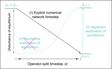
Figure 3: Illustration of the “operator-split” restoration of equilibrium abundance for an isotope. At the beginning of a network timestep that advances from $t_{n}$ to $t_{n+1}$ the abundance $y_{n}$ is assumed to take its equilibrium value $\bar{y}_{n}$. An explicit numerical timestep $\Delta t=t_{n+1}-t_{n}$ is then taken for all abundances, but with the contribution of equilibrated reaction groups removed from the fluxes. The isotope in question starts the timestep with its equilibrium abundance, but the numerical timestep will generally leave the abundance at a value $y_{n+1}$ that is not equal to the new equilibrium value $\bar{y}_{n+1}$ calculated from Eq. (21) because of its coupling to non-equilibrium reactions (the effect of the diagonal arrow). If the equilibrium approximation is to be maintained for the next timestep, the equilibrium value $\bar{y}_{n+1}$ must be restored before that timestep is taken. We could in principle restore the equilibrium by integrating numerically in a second step (the dashed blue line). However, we already know the result of that integration: it is given by Eq. (21), because by hypothesis $\Delta t$ is larger than the characteristic equilibration time for all reactions assumed to be in equilibrium. Thus we accomplish the second operator-split step algebraically rather than numerically by replacing the numerically-computed $y_{n+1}$ with $\bar{y}_{n+1}$ specified through Eq. (21) (the vertical arrow on the right side).

Establishment of equilibrium for individual reaction groups assumed to be in equilibrium within a single numerical timestep is fast compared with the timescale for reactions causing net changes in the abundances within a timestep. Thus, if we were to do the integration exactly, equilibrium for those reaction groups would be maintained during the timestep; but then we would have a highly-stiff numerical system combining fast and slow components. Our approximation replaces this actual evolution by a two-step process:

1. Evolve all network abundances by explicit forward differencing and asymptotic approximations, with the equilibrium reactions assumed to maintain their equilibrium (net zero) fluxes over the timestep. (This is what justifies removing the fluxes that are assumed equilibrated from the flux summation.)

2. Then, at the end of this first step, evolve all abundances assumed to be participating in equilibrium (which will have been disturbed by non-equilibrium processes in the first step) from their values computed at the end of the first step back to equilibrium values using Eq. (21), while holding non-equilibrium abundances constant.

Unlike the case for the usual operator-splitting between evolution of the hydrodynamics and evolution of the reaction network, this second step is not computed numerically by finite difference but is instead implemented through algebraic constraints. This is possible because the equilibrium assumption for a given reaction group means that it should evolve to the equilibrium solution before the end of the timestep. Therefore, since we know how the story ends, rather than integrating it explicitly we may simply replace the population at the end of the numerical timestep by its equilibrium value, calculated from Eq. (21). We gain from this separation of timescales and solution of the fast timescale by algebraic constraint rather than a finite-difference approximation a potentially large reduction of stiffness for the remaining part of the system that is integrated numerically. We shall demonstrate below that this can increase by orders of magnitude the maximum stable and accurate timestep for the overall integration in near-equilibrium conditions.

6.1.3 Complications in Realistic Networks

The complication for this basic idea in a realistic network with more than one reaction group in equilibrium is that there may be more than one computed equilibrium value for a given species that is assumed to be in equilibrium. This is because the equilibrium abundance Eq. (21) must be computed separately for each reaction group, and an isotope will generally be found in more than one reaction group. For example, assume an $\alpha$ network in which both reaction group I, defined by $\alpha+\mbox{${}^{28}$Si}\rightleftharpoons\mbox{${}^{32}$S}$, and reaction group II, defined by $\alpha+\mbox{${}^{40}$Ca}\rightleftharpoons\mbox{${}^{44}$Ti}$, are assumed to be in equilibrium. Then by our algorithm $Y_{\alpha}$ should assume its equilibrium value at the end of each timestep, but for each timestep there will be two values for the equilibrium abundance $\bar{Y}_{\alpha}$, corresponding to Eq. (21) solved for reaction group I and reaction group II, respectively. In the general case these values could be different, since the rates entering into Eq. (21) are different for the two reaction groups, and equilibrium within each reaction group is specified only to the tolerance implied by $\epsilon_{i}$ in Eq. (24). More realistically in larger networks a given isotope may be found in many reaction groups, some in equilibrium and some not, and for each group in equilibrium there will be a separate computed equilibrium value for the isotope.

However, by hypothesis the equilibrium abundances of a given isotope computed for each of its equilibrated reaction groups cannot be too different, since this would violate the equilibrium assumption. For example, consider the $\alpha$-network example from above. There is only one actual abundance $Y_{\alpha}$ in the network at a given time, and its value must be such that it satisfies simultaneously the equilibrium conditions for reaction group I and reaction group II, within the tolerances of Eq. (24); otherwise the equilibrium assumption would be invalidated. Therefore, restoration of equilibrium for a given isotope will correspond to setting its abundance to a compromise choice among each of the (similar) predicted equilibrium values for all equilibrated reaction groups in which it participates. This is a self-consistent approximation as long as the spread in possible equilibrium abundances remains consistent with the tolerances used to impose equilibrium in Eq. (24), for if this were not true it would suggest that the equilibrium assumption itself is suspect.

It is important conceptually that the use of “equilibrium assumption” as convenient shorthand in this discussion not be misinterpreted. The decision that a reaction group is in equilibrium is not an arbitrary choice but rather is made by the full network itself in each timestep. A reaction group is in equilibrium if it satisfies Eq. (24) for every species in the group, so the only arbitrary choices are the tolerances $\epsilon_{i}$. If the condition (24) is satisfied in a timestep for some reaction group, it is a statement by the network that in its current state the equilibration timescale for the reaction group has been found to be fast enough to maintain approximate equilibrium over the timestep.

6.2 Specific Methods for Restoring Equilibrium

As noted above, in realistic networks we must have a systematic way to restore equilibrium at the end of numerical timesteps since those reaction in equilibrium at the beginning of the timestep will generally be disturbed slightly away from equilibrium during the timestep by those reactions that are not in equilibrium. This effect is tiny for one reaction timestep, but will accumulate to unacceptable error over many timesteps if we do not correct for it in each timestep. In this section we outline three potential approaches to this problem. Although these approaches are general, it probably is easiest to understand them in the context of a specific application so we shall illustrate with a 4-isotope alpha network having species $\alpha$, ¹²C, ¹⁶O, and ²⁰Ne, that we already illustrated schematically in §5.1. Using explicit notation for the alpha network we include the reactions

$$\begin{array}[]{ll}0:&\ 3\alpha\rightleftharpoons\mbox{${}^{12}$C}\qquad 1:\ \alpha+\mbox{${}^{12}$C}\rightleftharpoons\mbox{${}^{16}$O}\\[2.0pt] 2:&\ \mbox{${}^{12}$C}+\mbox{${}^{12}$C}\rightleftharpoons\alpha+\mbox{${}^{20}$Ne}\qquad 3:\ \alpha+\mbox{${}^{16}$O}\rightleftharpoons\mbox{${}^{20}$Ne},\end{array}$$ (47)

which we shall reference below in terms of the number on the left side for each reaction, and the differential equations (34)–(37) governing the abundances then become

$$\dot{Y}_{\alpha}\hskip 0.0pt = \hskip 0.0pt-k^{(0)}_{\rm\scriptstyle f}Y_{\alpha}^{3}+k^{(0)}_{\rm\scriptstyle r}Y_{12}-k^{(1)}_{\rm\scriptstyle f}Y_{\alpha}Y_{12}+k^{(1)}_{\rm\scriptstyle r}Y_{16}$$ (48)

$$+k^{(2)}_{\rm\scriptstyle f}Y_{12}^{2}-k^{(2)}_{\rm\scriptstyle r}Y_{\alpha}Y_{20}-k^{(3)}_{\rm\scriptstyle f}Y_{\alpha}Y_{16}+k^{(3)}_{\rm\scriptstyle r}Y_{20}$$

$$\dot{Y}_{12}\hskip 0.0pt = \hskip 0.0ptk^{(0)}_{\rm\scriptstyle f}Y_{\alpha}^{3}-k^{(0)}_{\rm\scriptstyle r}Y_{12}-k^{(1)}_{\rm\scriptstyle f}Y_{\alpha}Y_{12}+k^{(1)}_{\rm\scriptstyle r}Y_{16}-k^{(2)}_{\rm\scriptstyle f}Y_{12}^{2}+k^{(2)}_{\rm\scriptstyle r}Y_{\alpha}Y_{20}$$ (49)

$$\dot{Y}_{16}\hskip 0.0pt = \hskip 0.0ptk^{(1)}_{\rm\scriptstyle r}Y_{\alpha}Y_{12}-k^{(1)}_{\rm\scriptstyle r}Y_{16}-k^{(3)}_{\rm\scriptstyle f}Y_{\alpha}Y_{16}+k^{(3)}_{\rm\scriptstyle r}Y_{20}$$ (50)

$$\dot{Y}_{20}\hskip 0.0pt = \hskip 0.0ptk^{(2)}_{\rm\scriptstyle f}Y_{12}^{2}-k^{(2)}_{\rm\scriptstyle r}Y_{\alpha}Y_{20}+k^{(3)}_{\rm\scriptstyle r}Y_{\alpha}Y_{16}-k^{(3)}_{\rm\scriptstyle r}Y_{20},$$ (51)

where we use a notation $Y(\mbox{${}^{12}$C})\equiv Y_{12}$ and so on, for the abundances (defined in Eq. (2)), and the rate parameters $k^{(n)}_{\rm\scriptstyle f}$ and $k^{(n)}_{\rm\scriptstyle r}$ refer to forward and reverse rates, respectively, for the reactions pairs labeled by the numbers on the left sides in Eq. (47). Thus $k^{(0)}_{\rm\scriptstyle f}$ is the rate parameter for $3\alpha\rightarrow\mbox{${}^{12}$C}$ and $k^{(3)}_{\rm\scriptstyle r}$ is the rate parameter for $\mbox{${}^{20}$Ne}\rightarrow\alpha+\mbox{${}^{16}$O}$.

6.2.1 Using Iteration to Reimpose Equilibrium Abundance Ratios

If we now impose equilibrium on the reaction $\alpha+\mbox{${}^{16}$O}\rightleftharpoons\mbox{${}^{20}$Ne}$ we obtain the constraint

$$Y_{\alpha}Y_{16}=\frac{k^{(3)}_{\rm\scriptstyle r}}{k^{(3)}_{\rm\scriptstyle f}}Y_{20}\equiv KY_{20}.$$ (52)

Inserting this constraint into Eqs. (48)–(51) eliminates the last two terms in each of Eqs. (48), (50), and (51), giving the reduced equations

$$\dot{Y}_{\alpha}\hskip 0.0pt = \hskip 0.0pt-k^{(0)}_{\rm\scriptstyle f}Y_{\alpha}^{3}+k^{(0)}_{\rm\scriptstyle r}Y_{12}-k^{(1)}_{\rm\scriptstyle f}Y_{\alpha}Y_{12}+k^{(1)}_{\rm\scriptstyle r}Y_{16}+k^{(2)}_{\rm\scriptstyle f}Y_{12}^{2}-k^{(2)}_{\rm\scriptstyle r}Y_{\alpha}Y_{20}$$ (53)

$$\dot{Y}_{12}\hskip 0.0pt = \hskip 0.0ptk^{(0)}_{\rm\scriptstyle f}Y_{\alpha}^{3}-k^{(0)}_{\rm\scriptstyle r}Y_{12}-k^{(1)}_{\rm\scriptstyle f}Y_{\alpha}Y_{12}+k^{(1)}_{\rm\scriptstyle r}Y_{16}-k^{(2)}_{\rm\scriptstyle f}Y_{12}^{2}+k^{(2)}_{\rm\scriptstyle r}Y_{\alpha}Y_{20}$$ (54)

$$\dot{Y}_{16}\hskip 0.0pt = \hskip 0.0ptk^{(1)}_{\rm\scriptstyle r}Y_{\alpha}Y_{12}-k^{(1)}_{\rm\scriptstyle r}Y_{16}$$ (55)

$$\dot{Y}_{20}\hskip 0.0pt = \hskip 0.0ptk^{(2)}_{\rm\scriptstyle f}Y_{12}^{2}-k^{(2)}_{\rm\scriptstyle r}Y_{\alpha}Y_{20}$$ (56)

This is the same number of equations as before, but these equations should now be less stiff than the original Eqs. (48)–(51) because the terms eliminated by substituting the equilibrium condition (52) are associated with the reaction pair that was first to come into equilibrium, precisely because it involves fast reactions. However, if we impose the equilibrium condition (52) at the beginning of a timestep, it generally will no longer be satisfied at the end of the timestep because the other reactions are not in equilibrium and will change the abundances of $\alpha$, ¹⁶O, and ²⁰Ne through non-equilibrium transitions. Thus, we must adjust the populations at the end of the timestep to reimpose the condition (52), assuming the equilibrium condition to still be satisfied for that reaction pair. In addition to the algebraic constraint (52), we have the condition

$$\Sigma_{X}\equiv\sum_{i}X_{i}=4Y_{\alpha}+12Y_{12}+16Y_{16}+20Y_{20}=1,$$ (57)

imposed by the requirement that the sum of the mass fractions be unity (conservation of nucleon number; see Eq. (2)). In contrast to the constraint (52), which is valid only if partial equilibrium conditions for the reaction $\alpha+\mbox{${}^{16}$O}\rightleftharpoons\mbox{${}^{20}$Ne}$ are satisfied, the constraint (57) is a conservation law that must always be satisfied. Thus, to reimpose equilibrium we have available two conditions, Eqs. (52) and (57).

We assume equilibrium at the beginning of the timestep in the $\alpha+\mbox{${}^{16}$O}\rightleftharpoons\mbox{${}^{20}$Ne}$ reaction (only); thus we advance the solution through a timestep $\Delta t$ by solving the reduced equations (53)–(56) using the explicit asymptotic algorithm [1]. Let us denote the (numerically computed) abundances at the end of this timestep by $\tilde{Y}_{i}=(\tilde{Y}_{\alpha},\tilde{Y}_{12},\tilde{Y}_{16},\tilde{Y}_{20})$. At the beginning of the timestep the condition (52) is satisfied, by hypothesis, but at the end of the timestep in general $\tilde{Y}_{\alpha}\tilde{Y}_{16}\neq K\tilde{Y}_{20}.$ But the assumption that $\alpha+\mbox{${}^{16}$O}\rightleftharpoons\mbox{${}^{20}$Ne}$ is in partial equilibrium implies (loosely) that the characteristic timescale $\tau$ for this reaction group must be less than the integration timestep. Thus, we may assume that if we had taken short enough timesteps the reaction pair $\alpha+\mbox{${}^{16}$O}\rightleftharpoons\mbox{${}^{20}$Ne}$ would have brought the populations for $Y_{\alpha}$, $Y_{16}$, and $Y_{20}$ back into equilibrium by the end of the actual timestep taken, and we use the algebraic conditions given by Eqs. (52) and (57) to reimpose $\alpha+\mbox{${}^{16}$O}\rightleftharpoons\mbox{${}^{20}$Ne}$ equilibrium at the end of the timestep. Eqs. (52) and (57) allow us to write

$$\begin{array}[]{l}F_{0}\equiv Y_{\alpha}-\frac{K}{Y_{16}}Y_{20}=0\qquad F_{1}\equiv Y_{16}-\frac{K}{Y_{\alpha}}Y_{20}=0\\ F_{2}\equiv Y_{\alpha}+3\tilde{Y}_{12}+4Y_{16}+5Y_{20}-\mbox{$\small\frac{1}{4}$}=0\end{array}$$ (58)

This may be written as the vector equation ${\bm{F}}=0$, which we can solve by Newton–Raphson iteration for the unknowns $Y_{\alpha}$, $Y_{16}$, and $Y_{20}$, starting the iteration from computed values $\tilde{Y}_{\alpha}$, $\tilde{Y}_{16}$, and $\tilde{Y}_{20}$, and taking $\tilde{Y}_{12}$ to be fixed at the computed value. In terms of the Jacobian matrix $\bm{J}$ defined by

$$\bm{J}\equiv\frac{\partial{\bm{F}}}{\partial{\bm{Y}}}\qquad{\bm{F}}=\left(\begin{array}[]{c}F_{0}\\ F_{1}\\ F_{2}\end{array}\right)\qquad{\bm{Y}}=\left(\begin{array}[]{c}Y_{\alpha}\\ Y_{16}\\ Y_{20}\end{array}\right)$$ (59)

a Newton–Raphson iteration step then corresponds to choosing an initial vector $\bm{Y}$, computing the corresponding values of $\bm{F}$ and $\bm{J}$, solving the matrix equation

$$\bm{J}\,\delta{\bm{Y}}=-\bm{F}$$ (60)

for the increment $\delta{\bm{Y}}$, and adding this increment to the original $\bm{Y}$ to get a corrected $\bm{Y}\rightarrow\bm{Y}+\delta{\bm{Y}}$. The corrected $\bm{Y}$ can then be used as the starting point for a second iteration, and so on until a convergence criterion is satisfied.

Because it involves a matrix solution, this method has the potential to spoil the linear scaling with network size that is attractive about explicit methods unless the matrix equations can be solved by means other than brute force. Because the matrices for large networks are expected to be sparse and well-conditioned, it is likely that solution methods giving scaling not too different from linear are possible, but this needs to be demonstrated for this method. For our tests we shall solve these matrix equations using standard matrix packages.

6.2.2 Use Iteration to Reimpose Equilibrium Abundances

As an alternative to restoring abundance ratios, we may seek to reimpose equilibrium by requiring that the individual abundances of all isotopes participating in equilibrium be set to their equilibrium values (21) at the end of their numerical timestep. Suppose that at some integration timestep there are $n$ reaction groups in equilibrium. There will be some number of isotopes $N$ participating in these reaction groups, with some isotopes participating in more than one equilibrated reaction group. Define a vector $\bm{Y}$ of the $N$ distinct isotopes that are participating in at least one equilibrated reaction group. If we assume that both $\alpha+\mbox{${}^{12}$C}\rightleftharpoons\mbox{${}^{16}$O}$ and $\alpha+\mbox{${}^{16}$O}\rightleftharpoons\mbox{${}^{20}$Ne}$ are in equilibrium for the network (47), $N=4$ and $n=2$, and the components of $\bm{Y}$ are

$$Y_{i}=\{Y_{\alpha},Y_{12},Y_{16},Y_{20}\}$$ (61)

where $Y_{12}=Y(\mbox{${}^{12}$C})$ and so on. Now define a vector $\bm{F}$ of normalized differences between the value of $Y_{i}$ at the end of the numerical timestep and its equilibrium value calculated from (21) at the end of the numerical timestep, and an entry imposing conservation of particle number, and require that it vanish. For the above example, we obtain the vector equation $\bm{F}=0$, with the components of $\bm{F}$ given by

$$F_{i}=\left\{\mbox{$\small\frac{Y_{\alpha}-\bar{Y}_{\alpha}^{(1)}}{\bar{Y}_{\alpha}^{(1)}}$},\mbox{$\small\frac{Y_{12}-\bar{Y}_{12}^{(1)}}{\bar{Y}_{12}^{(1)}}$},\mbox{$\small\frac{Y_{16}-\bar{Y}_{16}^{(1)}}{\bar{Y}_{16}^{(1)}}$},\mbox{$\small\frac{Y_{\alpha}-\bar{Y}_{\alpha}^{(3)}}{\bar{Y}_{\alpha}^{(3)}}$},\mbox{$\small\frac{Y_{16}-\bar{Y}_{16}^{(3)}}{\bar{Y}_{16}^{(3)}}$},\mbox{$\small\frac{Y_{20}-\bar{Y}_{20}^{(3)}}{\bar{Y}_{20}^{(3)}}$},\Sigma_{X}-1\right\},$$ (62)

where $Y_{i}$ denotes the actual abundance of species $i$ at the end of the numerical timestep and the computed equilibrium value of species $i$ at the end of the timestep is $\bar{Y}_{i}^{(j)}$, with the index $i$ labeling the position in the vector (61) and the index $j$ labeling the reaction group for which Eq. (21) is solved. The first three entries in the vector (62) are associated with restoring equilibrium in reaction group 1 and the next three entries are associated with restoring equilibrium in reaction group 3. Notice that the abundances $Y_{\alpha}$ and $Y_{16}$ appear more than once (twice each, for this example) in the vector $\bm{F}$. This is because these isotopes appear in reaction group 1 and in reaction group 3, both of which are assumed to be in equilibrium. For the last entry $\sum_{X}-1$ is defined by Eq. (57), and is a requirement that total nucleon number be conserved in the equilibrium restoration step.

Thus restoration of equilibrium at the end of the timestep, subject to conservation of particle number, corresponds to solving $\bm{F}(\bm{Y})=0$ for the vector $\bm{Y}$ (note that this vector contains only those isotopes that are part of reaction groups in equilibrium, not all of the isotopes in the network). As outlined in the previous section, the equation $\bm{F}(\bm{Y})=0$ can be solved iteratively for $\bm{Y}$ by choosing an initial guess for $\bm{Y}$, computing $\bm{F}(\bm{Y})$, solving the matrix equation (60) for the increment $\delta\bm{Y}$, computing the improved $\bm{Y}\rightarrow\bm{Y}+\delta\bm{Y}$, and then repeating until a convergence tolerance is satisfied. Since the equilibrium abundances for the isotopes are likely to change very slowly in successive timesteps, this Jacobian matrix may be expected to be almost constant between two successive timesteps, and it will not change in successive Newton–Raphson iterations since the equilibrium abundances are constant within a given timestep.

As for the method described in the previous section, a Newton–Raphson iteration on matrix equations is employed, so it will be highly desirable to solve these equations by means that retain the nearly linear scaling of the explicit method. From the discussion we see that for large networks with many reaction groups in equilibrium the matrices will be extremely sparse and only slightly changed in successive timesteps (and unchanged in successive Newton–Raphson iteration steps within a given timestep). We may expect that this structure lends itself to solutions with favorable scaling behavior in large networks, but that has not been investigated yet.

6.2.3 Reimpose Equilibrium Abundances by Averaging

The methods described in the previous two sections for restoring equilibrium at the end of numerical timesteps suffer from a certain level of redundancy because we have seen that in partial equilibrium the isotopic abundances in a reaction group are not independent but evolve according to a single timescale given by Eq. (23) (see the general discussion in §4.1). Thus, within a single reaction group specification of the equilibrium abundance of any one isotope, or of the progress variable associated with the reaction group, specifies the equilibrium abundance of all species in the group. Furthermore, within a single reaction group the evolution of the species in the group to equilibrium naturally conserves particle number, by virtue of constraints such as those of Eq. (15) that are listed for all five reaction group classes in Appendix A.

Let us exploit this by working with the progress variable $\lambda_{i}$ from each reaction group. If all the reaction groups were independent, then we could restore equilibrium for the progress variables for $n$ reaction groups in equilibrium simply by requiring

$$\bm{F}=\left(\begin{array}[]{c}\lambda_{1}-\bar{\lambda}_{1}\\ \lambda_{2}-\bar{\lambda}_{2}\\ \vdots\\ \lambda_{n}-\bar{\lambda}_{n}\end{array}\right)=0$$ (63)

where $\bar{\lambda}_{i}$ denotes the equilibrium value of $\lambda_{i}$ computed from Eq. (21) and relations like Eq. (22). Once the equilibrium value of $\lambda_{i}$ (or the abundance of any one of the isotopes in the reaction group) is computed, the equilibrium values for all other isotopes in the group than follow from constraints like Eq. (22) that are tabulated for all reaction group classes in Appendix A. No probability conservation constraint is included in Eq. (63) because each reaction group considered in isolation conserves particle number automatically in the evolution to equilibrium. The solution of Eq. (63) is then trivial, consisting of setting $\lambda_{i}=\bar{\lambda}_{i}$ for all $i$.

The simple considerations of the preceding paragraph cannot be used in the form presented: the reaction groups are generally not independent, because isotopes of the network appear typically in more than one reaction group, as we have discussed in §6.1.3. The equilibrium condition implies that the equilibrium abundances of a specific isotope computed for each of the reaction groups in which it is a member must be similar, but exact equality generally will not hold because of the finite tolerance $\epsilon_{i}$ used to test for equilibrium in Eq. (24). Thus, we restore equilibrium for each isotope participating in partial equilibrium at the end of a timestep by replacing its computed abundance with its equilibrium value averaged over all equilibrated reaction groups in which it participates. If the species $i$ is a member of $M$ equilibrated reaction groups, its restored equilibrium value at the end of the timestep is

$$\bar{Y}_{i}=\frac{1}{M}\sum_{j}^{M}\bar{Y}_{i}^{(j)}.$$ (64)

where the equilibrium abundances $\bar{Y}_{i}^{(j)}$ are computed for each of the reaction groups from Eq. (21).

There is one further issue: although the evolution to equilibrium for individual reaction groups conserves particle number, the averaging procedure of Eq. (64) over multiple reaction groups will introduce a fluctuation in the particle number since the chosen value of $\bar{Y}_{i}$ computed from the average will generally differ from the individual $\bar{Y}_{i}^{(j)}$ that were computed conserving particle number. This difference will be very small in any one timestep, but can accumulate to unacceptable failure of particle number conservation for a long integration. Thus, for each timestep, after equilibrium has been restored through Eq. (64) we recompute the total particle number in the network (now summing over all isotopes, whether participating in equilibrium or not), compare it with the total particle number at the beginning of the timestep, and rescale all $Y_{i}$ in the network by a multiplicative factor that restores the particle number to its initial value.

We have shown in a variety of comparisons that this procedure for restoring equilibrium works very well, giving results (isotopic abundances and timestepping profile) that are essentially identical to those of the iterative matrix algorithms discussed in the previous two sections. The advantage of the present approach is simplicity and automatically-favorable scaling with network size. The restoration of equilibrium involves only a summation over reaction groups to compute averages, followed by a multiplicative renormalization by a scalar. Thus there are no matrix inversions and no Newton–Raphson iterations, so this algorithm for restoring equilibrium is very simple to implement and should scale linearly with the size of the network, straight out of the box. All of the following examples were computed using this averaging algorithm.

7 A Simple Adaptive Timestepper

For testing the algorithms described here an adaptive timestepper has been employed that is described in more detail in Refs. [1, 2, 13]. This timestepper is far from optimized but it leads to stable and accurate results for the varied astrophysical networks that have been tested. Thus it is adequate for our primary task here, which is to establish whether explicit partial equilibrium methods can even compete with implicit methods for stiff networks.

8 Toy Models for Partial Equilibrium

As a first illustration of using the partial equilibrium methods developed in the preceding sections, we take a very simple thermonuclear network including only three isotopes, ⁴He ($\alpha$-particles), ¹²C, and ¹⁶O, connected by the reactions $3\alpha\rightleftharpoons\mbox{${}^{12}$C}$ and $\alpha+\mbox{${}^{12}$C}\rightleftharpoons\mbox{${}^{16}$O}.$ Thus we have a total of four reactions in two reaction groups, with $3\alpha\rightleftharpoons\mbox{${}^{12}$C}$ belonging to reaction group class C and $\alpha+\mbox{${}^{12}$C}\rightleftharpoons\mbox{${}^{16}$O}$ belonging to reaction group class B. The partial equilibrium formulas for both cases have been summarized in A. This is an extremely simple network but we shall see that it demonstrates in a rather transparent way most of the essential features of a partial equilibrium calculation.

Figure 4

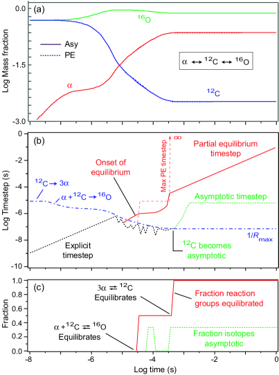
Figure 4: The effect of imposing partial equilibrium on integration timesteps for the network $\alpha\rightleftharpoons\mbox{${}^{12}$C}\rightleftharpoons\mbox{${}^{16}$O}$ at a constant temperature of $5\times 10^{9}$ K and constant density $1\times 10^{8}\mbox{\ g\,cm}^{-3}$, assuming initial mass fractions of $0.50$ for ¹²C and ¹⁶O. Reaction rates were taken from standard compilations [12]. (a) Mass fractions as a function of time. The results are almost indistinguishable between the purely asymptotic calculation (Asy) and the asymptotic plus partial equilibrium calculation (PE). (b) The purely-explicit integration timestep (black dotted), the asymptotic timestep (green dotted), the partial equilibrium timestep (solid red), the approximate maximum explicit timestep for the asymptotic calculation (dash-dotted blue), and the maximum stable timestep for the partial equilibrium calculation (dashed red). (c) The fraction of isotopes that are asymptotic and the fraction of reaction groups that are equilibrated as a function of time. The dotted green curves in the middle and bottom figures refer to the results one obtains with the explicit asymptotic method if partial equilibrium is not imposed.

illustrates a simulation with this network at a constant temperature of $5\times 10^{9}$ K and constant density $1\times 10^{8}\mbox{\ g\,cm}^{-3}$. This calculation employs the explicit asymptotic method [1], but tries to impose partial equilibrium if the abundances of all reactions in a reaction group are within $0.01$ of their equilibrium abundances. The dash-dotted blue curve labeled $1/R_{\mbox{\scriptsize max}}$ estimates the maximum stable fully-explicit timestep as the inverse of the current fastest rate in the network. This curve is set by the $\mbox{${}^{12}$C}\rightarrow 3\alpha$ reaction initially, but by the $\alpha+\mbox{${}^{12}$C}\rightarrow\mbox{${}^{16}$O}$ reaction after $\log t\sim-7.5$.

First consider a purely asymptotic approximation. At the beginning the maximum accurate timestep is smaller than the maximum stable explicit timestep, so the algorithm takes explicit timesteps with a size set by accuracy and not stability considerations (which we arbitrarily cap for this example at $dt\sim 0.1t$ to ensure accuracy). Near $\log t=-5.2$ the explicit timestep becomes equal to the maximum stable explicit timestep (intersection of dash-dotted blue and dotted black curves), which is decreasing with time at this point because the rate for $\alpha+\mbox{${}^{12}$C}\rightarrow\mbox{${}^{16}$O}$ is increasing with time. No isotopes are yet asymptotic, so the explicit timestep begins to decrease in order to remain below the dash-dotted blue curve and thus maintain stability, with the fluctuations in the timestep curve representing the attempts by the timestepping algorithm to increase the timestep being thwarted by the stiffness instability. But around $\log t=-3.5$ one of the isotopes (¹²C) becomes asymptotic and the timestep begins to increase rapidly over the explicit stability limit. However, the explicit asymptotic algorithm is unable to take large enough timesteps to make more isotopes asymptotic and the asymptotic timestep saturates at late times near $dt\sim 1\times 10^{-5}$ s (dotted green curve).

On the other hand, for the asymptotic plus PE calculation we proceed as for the purely asymptotic calculation until at $\log t\sim-4.4$ the $\alpha+\mbox{${}^{12}$C}\rightleftharpoons\mbox{${}^{16}$O}$ reaction is determined by the network to satisfy the partial equilibrium condition and the net flux from this pair of reactions is removed from the numerical integration by the PE algorithm. Because of the removal of these fast components, the maximum stable timestep for the PE calculation (dashed red curve in Fig. 4(b), corresponding to the inverse of the fastest timescale remaining in the numerical integration) begins to increase relative to that for the asymptotic calculation (dash-dotted blue curve). In response, the PE integration step size (solid red curve in Fig. 4(b)) also begins to increase until at $\log t\sim-3.4$ it is about 100 times larger than the purely asymptotic timestep. At this point, the network determines that the $3\alpha\rightleftharpoons\mbox{${}^{12}$C}$ reaction group also satisfies the partial equilibrium condition and removes this pair of reactions from the numerical integration too. Now, since there are only two equilibrium reaction groups in our simple network and they have both been removed by the PE algorithm, the numerical integrator is effectively solving the set of equations $d\bm{Y}=0$. Since all timescales have now been removed from the numerical integration by the PE algorithm, there is no stiffness instability at all and the maximum stable timestep (dashed red curve) goes to infinity.

Provided that the two reaction groups remain in equilibrium, we are now free to take timesteps limited only by accuracy. Accordingly the PE timestep increases rapidly and once again becomes equal to an upper limit of $dt\sim 0.1t$ imposed by our arbitrary overall accuracy constraint (solid red curve). Thus, after a network evolution time of one second the partial equilibrium timestep is approximately four orders of magnitude larger than that for the explicit asymptotic algorithm, with the calculated isotopic abundances as a function of time being indistinguishable in the two cases. This translates into a total integration time that is 400 times faster for the asymptotic plus partial equilibrium calculation versus the purely asymptotic calculation in the example of Fig. 4.

A deeper understanding of the factors that determine the timesteps in Fig. 4 may be obtained by consulting Fig. 5,

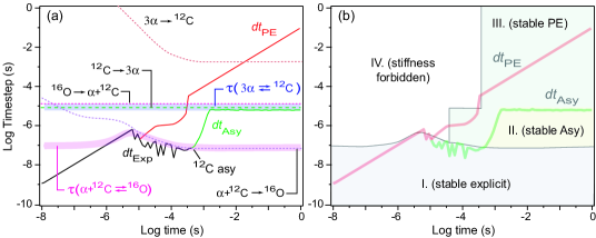
Figure 5: (a) Equilibration and reaction timescales for Fig. 4. (b) Stiffness stability domains implied by the equilibration timescales in part (a).

which displays all timescales relevant for the problem as a function of time. Figure 5(a) shows the timescales defined by the inverse of the reaction rates for all reactions in the network (dotted and dashed curves), the timescales $\tau$ of Eq. (23) for establishing equilibrium for the two reaction groups in this calculation (magenta and blue bands), and the integration timestepping for various methods (solid curves). The differential equations to be solved are those of Eqs. (48)–(51) with terms involving ²⁰Ne removed:

$$\dot{Y}_{\alpha}\hskip 0.0pt = \hskip 0.0pt-k^{(0)}_{\rm\scriptstyle f}Y_{\alpha}^{3}+k^{(0)}_{\rm\scriptstyle r}Y_{12}-k^{(1)}_{\rm\scriptstyle f}Y_{\alpha}Y_{12}+k^{(1)}_{\rm\scriptstyle r}Y_{16}$$ (65)

$$\dot{Y}_{12}\hskip 0.0pt = \hskip 0.0ptk^{(0)}_{\rm\scriptstyle f}Y_{\alpha}^{3}-k^{(0)}_{\rm\scriptstyle r}Y_{12}-k^{(1)}_{\rm\scriptstyle f}Y_{\alpha}Y_{12}+k^{(1)}_{\rm\scriptstyle r}Y_{16}$$ (66)

$$\dot{Y}_{16}\hskip 0.0pt = \hskip 0.0ptk^{(1)}_{\rm\scriptstyle r}Y_{\alpha}Y_{12}-k^{(1)}_{\rm\scriptstyle r}Y_{16}-k^{(3)}_{\rm\scriptstyle f}Y_{\alpha}Y_{16}$$ (67)

In the explicit asymptotic calculation (where we ignore the role of the equilibrium timescales denoted by the magenta and blue bands) we see that the timestep is rigidly limited by the inverse rate for $\alpha+\mbox{${}^{12}$C}\rightarrow\mbox{${}^{16}$O}$ (dashed purple curve) until ¹²C becomes asymptotic (labeled ¹²C asy). This partially lifts the timestepping restriction because Eq. (65) and its source terms for $\alpha+\mbox{${}^{12}$C}\rightleftharpoons\mbox{${}^{16}$O}$ are then removed from the numerical integration. However, since no other isotopes become asymptotic, the numerical integration is unable to get past the ceiling imposed by the timescales associated with $\mbox{${}^{12}$C}\rightarrow 3\alpha$ and $\mbox{${}^{16}$O}\rightarrow\alpha+\mbox{${}^{12}$C}$ that remain in Eqs. (66)–(67) and the asymptotic timestep saturates around $10^{-5}$ s at late times.

In contrast, the partial equilibrium method is able to remove all timescales in all three equations associated with the reaction group $\alpha+\mbox{${}^{12}$C}\rightleftharpoons\mbox{${}^{16}$O}$ when the timestep $dt$ is comparable to the magenta band denoting $\tau(\alpha+\mbox{${}^{12}$C}\rightleftharpoons\mbox{${}^{16}$O})$. This complete removal of a set of fast timescales replaces the original problem with one that is less stiff. That permits the PE method to increase its timestep sufficiently that $dt$ quickly reaches the equilibrium timescale associated with $3\alpha\rightleftharpoons\mbox{${}^{12}$C}$ (blue band) and removes completely all timescales associated with this reaction group too, leaving an integration problem having no stiffness limitation on the explicit timestep.

An even simpler picture of the relationship between asymptotic and partial equilibrium approximations emerges if we consider the evolution of a single reaction group. In Fig. 6(a),

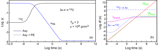
Figure 6: Equilibration of the single reaction group $3\alpha\rightleftharpoons\mbox{${}^{12}$C}$. (a) Mass fractions in asymptotic and asymptotic plus partial equilibrium approximation. (b) Timescales and integration timesteps. The dashed curves are the timescales set by the inverses of the reaction rates; the dotted red curve is the equilibration timescale (23) for the reaction group. The solid green curve is the integration timestepping for an asymptotic approximation and the solid red curve is the timestepping for an asymptotic plus partial equilibrium approximation.

by evolving a single reaction group consisting of the triple-alpha reaction and its inverse, we see clearly the role of the individual reaction timescales and the timescale for approach to equilibrium of $3\alpha\rightleftharpoons\mbox{${}^{12}$C}$ in setting the timestepping for asymptotic integration. For accuracy in this example, we have arbitrarily limited the integration timestep to $dt\leq 0.1t$. As illustrated in Fig. 6(b), initially, the largest stable fully-explicit timestep is governed by the inverse of the rate for the $3\alpha\rightarrow\mbox{${}^{12}$C}$ reaction. Until $\log t\sim 4$, the largest accurate timestep lies below this timescale, so there is no stiffness limitation on the explicit integration. At around $\log t\sim 4$ the ⁴He ($\alpha$ particle) becomes asymptotic and the asymptotic timestep begins to exceed the limit set by the $3\alpha\rightarrow\mbox{${}^{12}$C}$ reaction by a small amount. However, the other isotope in the network, ¹²C, never satisfies the asymptotic condition over the entire range of integration. Thus, the asymptotic method is never able to remove completely the stiffness timescales set by the $3\alpha\rightleftharpoons\mbox{${}^{12}$C}$ reactions (since they will remain at all times in the differential equation for ¹²C, which must be integrated numerically). Thus the asymptotic-method integration timestep saturates at late times near the timescale set by the inverse of the rate for $3\alpha\rightarrow\mbox{${}^{12}$C}$.

On the other hand, in the asymptotic plus PE calculation the reaction group $3\alpha\rightleftharpoons\mbox{${}^{12}$C}$ becomes equilibrated according to the criteria of Eq. (24) at about the time the equilibrium timescale for the reaction group (shown as the magenta band) crosses the $dt$ curve near $\log t\sim 3$. Since the reaction group is now assumed to be in equilibrium, all flux terms associated with both $3\alpha\rightarrow\mbox{${}^{12}$C}$ and $\mbox{${}^{12}$C}\rightarrow 3\alpha$ are removed from the numerical integration and the numerical integrator must solve the system $dY_{\alpha}/dt=dY_{12}/dt=0$. Since all timescales have been removed from the network, the corresponding integration timestep is set only by accuracy criteria. As a result, the partial equilibrium integration in Fig. 6 is more than 300,000 times faster than the asymptotic integration of the same system, with essentially identical results.

Similar considerations apply in more complex networks and it is useful to view the timescales of Fig. 5(a) or Fig. 6(b) as establishing stiffness stability domains in the $dt$ versus $t$ plane that are illustrated in Fig. 5(b). Thus, a fully-explicit integration is restricted by stability considerations to the lower domain marked I, an asymptotic (or QSS) calculation is restricted to domains I and II, an asymptotic or QSS plus partial equilibrium calculation is restricted to domains I, II, and III, and all of these methods would be unstable in domain IV. However, as illustrated in Fig. 5(b), if we are sufficiently clever we can push domain IV far enough into the upper left corner of the $dt-t$ plane that it plays little practical role because the instability domain corresponds to timesteps that would be undesirable from an accuracy point of view.

The examples displayed in Figs. 5 and 6 are not very complex and it should be not at all surprising that the description of the system becomes simple and the stable timesteps large at later times, since the mass fraction curves become almost constant in this region. But that is the whole point of the partial equilibrium approach: near equilibrium the system is complicated when viewed in terms of competing independent reactions, but becomes simple when viewed in terms of groups of reactions coming into equilibrium and thus bringing the whole system into equilibrium. These examples illustrate for some very simple networks, but the same principles will apply to the more complex networks to which we now turn.

9 Tests on Some Thermonuclear Alpha Networks

We have tested the partial equilibrium algorithm described in earlier sections in a variety of thermonuclear alpha networks. In this section we give some representative examples of those calculations. Because they are extremely challenging reaction network problems to solve, we shall concentrate on examples representative of conditions expected in Type Ia supernova simulations (temperatures in the range $10^{7}$–$10^{10}$ K, densities in the range $10^{7}$–$10^{9}$ g cm^-3, and initial equal mass fractions of ¹²C and ¹⁶O). Such conditions lead quickly to high degrees of equilibration in the approach to QSE (quasi-statistical equilibrium) and NSE (nuclear statistical equilibrium), and are a stringent test of partial equilibration methods. Our long-term goal is application of these methods to larger networks, but an alpha network provides a highly-stiff test system that is small enough to allow significant insight into how the algorithm functions. We also note as a practical matter that the most ambitious published calculations for thermonuclear networks coupled to hydrodynamical simulations have employed alpha networks.

The reactions and corresponding reaction groups used in the calculations are displayed in Table 4.

Table 4: Reactions of the alpha network for partial equilibrium calculations. The reverse reactions such as $\mbox{${}^{20}$Ne}\rightarrow\alpha+\mbox{${}^{16}$O}$ are photodisintegration reactions, $\gamma+\mbox{${}^{20}$Ne}\rightarrow\alpha+\mbox{${}^{16}$O}$, with the photon $\gamma$ suppressed in the notation.

• Group	Class	Reactions	Members
  1	C	$3\alpha\rightleftharpoons\mbox{${}^{12}$C}$	4
  2	B	$\alpha+\mbox{${}^{12}$C}\rightleftharpoons\mbox{${}^{16}$O}$	4
  3	D	$\mbox{${}^{12}$C}+\mbox{${}^{12}$C}\rightleftharpoons\alpha+\mbox{${}^{20}$Ne}$	2
  4	B	$\alpha+\mbox{${}^{16}$O}\rightleftharpoons\mbox{${}^{20}$Ne}$	4
  5	D	$\mbox{${}^{12}$C}+\mbox{${}^{16}$O}\rightleftharpoons\alpha+\mbox{${}^{24}$Mg}$	2
  6	D	$\mbox{${}^{16}$O}+\mbox{${}^{16}$O}\rightleftharpoons\alpha+\mbox{${}^{28}$Si}$	2
  7	B	$\alpha+\mbox{${}^{20}$Ne}\rightleftharpoons\mbox{${}^{24}$Mg}$	4
  8	D	$\mbox{${}^{12}$C}+\mbox{${}^{20}$Ne}\rightleftharpoons\alpha+\mbox{${}^{28}$Si}$	2
  9	B	$\alpha+\mbox{${}^{24}$Mg}\rightleftharpoons\mbox{${}^{28}$Si}$	4
  10	B	$\alpha+\mbox{${}^{28}$Si}\rightleftharpoons\mbox{${}^{32}$S}$	2
  11	B	$\alpha+\mbox{${}^{32}$S}\rightleftharpoons\mbox{${}^{36}$Ar}$	2
  12	B	$\alpha+\mbox{${}^{36}$Ar}\rightleftharpoons\mbox{${}^{40}$Ca}$	2
  13	B	$\alpha+\mbox{${}^{40}$Ca}\rightleftharpoons\mbox{${}^{44}$Ti}$	2
  14	B	$\alpha+\mbox{${}^{44}$Ti}\rightleftharpoons\mbox{${}^{48}$Cr}$	2
  15	B	$\alpha+\mbox{${}^{48}$Cr}\rightleftharpoons\mbox{${}^{52}$Fe}$	2
  16	B	$\alpha+\mbox{${}^{52}$Fe}\rightleftharpoons\mbox{${}^{56}$Ni}$	2
  17	B	$\alpha+\mbox{${}^{56}$Ni}\rightleftharpoons\mbox{${}^{60}$Zn}$	2
  18	B	$\alpha+\mbox{${}^{60}$Zn}\rightleftharpoons\mbox{${}^{64}$Ge}$	2
  19	B	$\alpha+\mbox{${}^{64}$Ge}\rightleftharpoons\mbox{${}^{68}$Se}$	2

We use the standard REACLIB library [12] for all rates except for three of the heavy-ion reactions (corresponding to reaction groups 3, 5, and 6 in the table) which have inverse reactions that are absent from the REACLIB compilation and were taken from Ref. [14]. For typical Type Ia supernova conditions the rates for the capture and photodisintegration reactions in Table 4 become comparable and as large as $\sim 10^{10}-10^{12}\mbox{\ s}^{-1}$. The corresponding maximum stable fully-explicit integration timestep will be of order the inverse of the maximum rate in the network, so timesteps as short as $\sim 10^{-12}\mbox{\ s}$ may be required for stability of a fully-explicit integration. On the other hand, the characteristic physical timescale for the primary Type Ia explosion mechanism is of order one second. Thus integration of the alpha network coupled to a hydrodynamics simulation of a Type Ia explosion could require $10^{12}$ or more explicit network integration timesteps, which is obviously not practical and indicates graphically that this is an extremely stiff system.

9.1 Comparisons of Explicit and Implicit Integration Speeds

We shall be comparing explicit and implicit methods using codes that are at very different stages of development and optimization. Thus, they cannot simply be compared directly with each other. We assume that for codes at similar levels of optimization the primary difference between explicit and implicit methods would be in the extra time spent in implicit-method matrix operations. Hence, if the fraction of time spent on linear algebra is $f$ for an implicit code, we assume that an explicit code at a similar level of optimization could compute a timestep faster by a factor of $F=1/(1-f)$. Factors $F$ have been tabulated in Ref. [1] for several networks. Then we may compare roughly the speed of explicit versus implicit codes (possibly at different levels of optimization) by multiplying $F$ by the ratio of implicit to explicit integration steps required for a given problem. This procedure has obvious uncertainties, and likely underestimates the speed of an optimized explicit versus optimized implicit code, but will give a useful lower limit on how fast the explicit calculation can be relative to implicit methods.

9.2 Constant Intermediate-Temperature, Low-Density Example

A calculation for constant $T_{9}=5$ and density of $1\times 10^{7}\mbox{\ g\,cm}^{-3}$ in an alpha network is shown in Fig. 7.

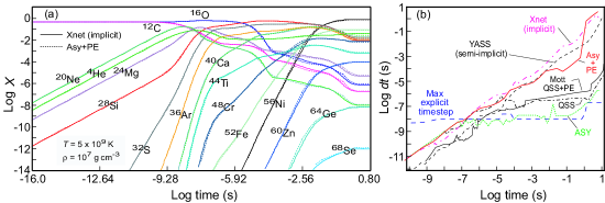
Figure 7: Partial equilibrium calculation for constant $T_{9}=5$ and $\rho=1\times 10^{7}\mbox{\ g\,cm}^{-3}$ alpha network. (a) Mass fractions. Solid lines are implicit calculations (Xnet) and dashed lines are asymptotic + PE calculations. (b) Integration timesteps for several different integration methods. Magenta dash-dot is the implicit code Xnet [15], black dashed is the semi-implicit code YASS [16] (reproduced from from Ref. [10]), solid red is the current asymptotic plus partial equilibrium result, solid black is the QSS plus partial equilibrium calculation reproduced from Ref. [10], black dash-dot is a QSS calculation using the formalism of Ref. [2], dotted green is an asymptotic calculation using the formalism in Ref. [1], and dashed blue is the estimated maximum stable fully-explicit timestep.

This network has 16 isotopes with 48 reactions connecting them, and a total of 19 reaction groups that can separately come into equilibrium. For this and all other calculations equilibrium conditions were imposed using Eq. (24), with a constant value $\epsilon_{i}=0.01$ for the tolerance parameter. The calculated asymptotic plus partial equilibrium (Asy + PE) mass fractions are compared with those of a standard implicit code in Fig. 7(a). There are small discrepancies in localized regions, especially for some of the weaker populations, but for the most part the agreement is rather good. Although we shall generally display mass fractions down to $10^{-14}$ in our examples for reference purposes, it is important to note that for reaction networks coupled to hydrodynamics only larger mass fractions (those larger than say $\sim 10^{-2}-10^{-3}$) are likely to have significant influence on the hydrodynamics. Thus, the largest discrepancies between mass fractions calculated by PE and implicit methods in Fig. 7(a) mostly imply uncertainties in the total mass being evolved by the network of less than one part in a million, which would be completely irrelevant in a coupled hydrodynamical simulation.

Timestepping for various integration methods is illustrated in Fig. 7(b), where there are several interesting features to discuss.

1. The PE timestepping is seen to compare rather favorably with standard fully-implicit and semi-implicit codes. The PE calculation required 3941 integration steps while the implicit code Xnet required only 600 steps, but this factor of 6.5 timestepping advantage is offset substantially by the expectation that for a 16-isotope network an explicit calculation should be $\sim 3$ times faster than the implicit calculation for each timestep [1]. Thus we conclude that for fully-optimized codes the implicit calculation would be perhaps several times faster for this example. The semi-implicit timestepping curve was reproduced from another reference but a comparison of the curves in Fig. 7(b) suggests that an optimized partial equilibrium code is likely to be at least as fast as the semi-implicit YASS code for this example.

2. The Asy + PE and implicit timestepping are seen to be many orders of magnitude better at late times than the results of our purely asymptotic (Asy) and purely quasi-steady-state (QSS) calculations, which are based on the formalisms discussed in Refs. [1, 2]. The reason is apparent from Fig. 8. For times later than about $\log t=-6$, significant numbers of reaction groups come into partial equilibrium, which asymptotic and QSS methods are not designed to handle.

3. The earlier application by Mott et al [10] of a QSS plus partial equilibrium calculation for this system lags orders of magnitude behind the current implementation of asymptotic plus partial equilibrium in timestepping at late times. In fact, the timestepping from Ref. [10] is only a little better than that of the pure QSS results from the present paper.

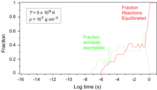
Figure 8: Fraction of reactions that are treated as being in equilibrium as a function of integration time for the calculation of Fig. 7 (solid red curve). Also shown is the fraction of isotopes that become asymptotic in the PE calculation (dotted green curve).

In Fig. 9

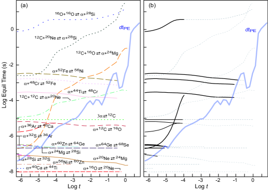
Figure 9: Timestepping and partial equilibrium timescales associated with the calculation in Fig. 7. (a) The equilibrium timescales, with the reactions removed for times after they become equilibrated in the PE calculation. (b) As for part (a), but with labels suppressed and with time ranges for which equilibrium reactions have been partially removed by the asymptotic approximation indicated by dashed curves. The heavy, dark curves indicate times for which the corresponding equilibrium timescale has been removed neither by asymptotic nor PE approximations and therefore is fully operative in producing stiffness. These curves clearly have a large influence on the maximum timestep $dt_{\mbox{\scriptsize PE}}$ that the PE calculation is able to take.

we display the partial equilibrium timescales of Eq. (23) that are associated with the calculation of Fig. 7, with the reactions that are removed by partial equilibrium or asymptotic considerations indicated (compare with the simpler earlier example in Fig. 5). In Fig. 9(a) each reaction has been removed from the graph when it reaches equilibration. In Fig. 9(b) we also indicate in dashed gray those reactions that have been at least partially removed from the numerical integration by isotopes becoming asymptotic, or ranges of times for reactions in which reactants have very small concentration and therefore make only small contribution. The complete removal of reactions by partial equilibration and the partial removal of reactions by asymptotic conditions clearly play a significant role in determining the envelope of the maximum stable and accurate partial equilibrium timestep, as seen in Fig. 9(b).

9.3 Constant Higher-Temperature, Intermediate-Density Example

A calculation for constant $T_{9}=7$ and density of $1\times 10^{8}\mbox{\ g\,cm}^{-3}$ in an alpha network is shown in Fig. 10.

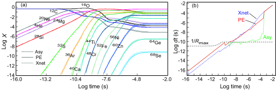
Figure 10: Partial equilibrium calculation for constant $T_{9}=7$ and $\rho=1\times 10^{8}\mbox{\ g\,cm}^{-3}$ alpha network. (a) Mass fractions. Solid curves are asymptotic + PE, dashed curves are asymptotic, and dotted curves are implicit (Xnet). (b) Integration timesteps for the present asymptotic plus partial equilibrium calculation (solid red), the implicit code Xnet [15] (dotted blue), and the asymptotic method of Ref. [1] (dashed green).

Again we see extremely good agreement among the mass fractions calculated by an implicit method, the asymptotic method, and the asymptotic plus partial equilibrium method. The timesteps for the partial equilibrium and implicit methods are quite similar, with the implicit method requiring 510 integration steps and the partial equilibrium method 506 integrations steps. An optimized explicit code can probably evaluate a timestep $\sim 3$ times faster than an implicit code for a 16-isotope network [1] and we conclude that for similarly-optimized codes the partial equilibrium calculation would be slightly faster. In contrast, the asymptotic method lags far behind at late times, because the equilibration becomes significant after $10^{-8}$ s, with the fraction of reactions that are equilibrated reaching 100% for times later than $10^{-4}$ s. As a consequence, the integration of Fig. 10 required more than two million purely-asymptotic integration steps.

9.4 Example with a Hydrodynamical Profile

The preceding two examples employed alpha networks at extreme but constant temperature and density. A partial equilibrium calculation using a hydrodynamical profile with the dramatic temperature rise characterizing a thermonuclear runaway in a Type Ia supernova simulation is illustrated in Fig. 11.

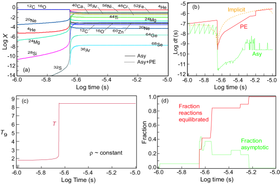
Figure 11: Asymptotic, PE, and implicit calculations with an alpha network for Type Ia supernova conditions. (a) Mass fractions. (b) Integration timesteps. (c) Hydrodynamic profile [17]. (d) Fraction of isotopes asymptotic and partially-equilibrated reactions.

The thermonuclear runaway in degenerate white-dwarf matter subjects the reaction network to extreme conditions in this example: the difference between the fastest and slowest reaction timescales is more than 11 orders of magnitude and during the thermonuclear flash the temperature increases by 6.6 billion K in only $1.5\times 10^{-7}$ s (a rate of temperature change corresponding to $4.4\times 10^{16}\mbox{\ K/s}$). The asymptotic plus PE method required 712 steps to integrate this problem, compared with 524 steps for the implicit calculation, suggesting that an optimized explicit code would be about twice as fast as the implicit code because it can compute a timestep about three times faster. In contrast, the purely asymptotic calculation gave accurate results but required almost 190,000 integration steps for the time range shown.

As may be seen from Fig. 11(d), the partial equilibrium calculation becomes completely equilibrated after $\log t\sim-5.2$ and after that time the PE timesteps are limited only by accuracy. Choosing to restrict the subsequent timesteps to $dt=0.3t$, continuation of the PE (or implicit) integration of Fig. 11 until the characteristic timescale for the supernova explosion of $\sim 1$ s requires only a few tens of additional integration steps. In contrast, if the asymptotic integrator continued to take the timesteps it is taking at the end of the calculation in Fig. 11, it would require more than a billion additional integration steps to reach the full physical timescale for the supernova.

9.5 Synopsis

The three examples shown above are representative of a number of problems that we have investigated with the new asymptotic plus partial equilibrium methods. Our general conclusion is that for alpha networks under the extreme conditions corresponding to a Type Ia supernova explosion the asymptotic plus partial equilibrium algorithm is capable of giving timestepping that is orders of magnitude better than asymptotic or QSS approximations alone when the system approaches equilibrium, that these timesteps are often competitive with current implicit and semi-implicit codes, and that they are orders of magnitude faster than previous attempts to apply such explicit methods to extremely stiff thermonuclear networks.

10 Improving the Speed of Explicit Codes

The preceding discussion, and that of Refs. [1, 2], have assumed that we can compare (approximately) the relative speed of explicit and implicit methods that are presently implemented with different levels of optimization by comparing the number of integration timesteps required to do a particular problem with each method. The assumption of this comparison is that once the matrix overhead associated with implicit methods is factored out, the rest of the work required in a timestep (computing rates and fluxes, and so on) is similar for explicit and implicit methods. While this is useful for a first estimation, it should not be viewed yet as a quantitative comparison of the speed of implicit and explicit methods for two basic reasons. (1) The current timestep routines for implicit methods and the explicit methods presented here are at very different levels of algorithmic optimization. (2) Because the timestep routines are not yet equivalently optimized, we have not made a systematic study of optimal timestepping parameters for either the implicit or explicit methods. Thus, the results presented here should be interpreted as indicating that for the problems investigated explicit methods can take stable and accurate timesteps that are comparable to those of implicit methods. Further work will be required to determine whether implicit or explicit methods are faster and by how much for specific problems.

There are at least three reasons why the integration speed for explicit methods may potentially be even faster than that estimated by such a procedure in this paper and in Refs. [1, 2].

First, in this paper we have emphasized partial equilibrium methods in league with asymptotic approximations. But in Ref. [2] we presented evidence that quasi-steady-state (QSS) methods give results comparable to asymptotic methods, but often with timesteps that can be as much as an order of magnitude larger. Thus, we may expect that a QSS plus partial equilibrium approximation could give even better timestepping than the examples shown here. We have not yet investigated this possibility systematically.

Second, we have seen that the timestepping algorithm employed in this paper and in Refs. [1, 2] is not very optimized. On the one hand, results such as those exhibited in Fig. 9(b) suggest that our timestepper is tracing qualitatively the explicit-integration stability boundary. But that same figure suggests that in many regions explicit timesteps as much as an order of magnitude larger could still be stable. Thus, it is possible that we have over-estimated the number of integration steps required by our explicit methods in the examples discussed in this paper because of an adequate but not optimized timestepper. This possibility also remains to be investigated.

Third, and potentially of most importance, our demonstration that algebraically-stabilized explicit methods may in fact be viable for large, extremely-stiff networks implies new considerations with respect optimization. For standard implicit methods, the most effective optimizations involve improving the numerical linear algebra, since in large networks more than 90% of the computing time for implicit methods can be consumed by matrix inversions. But with algebraically-stabilized explicit methods the bulk of the computing time for large networks is spent in computing the rates. Thus, the most effective optimization for our explicit methods lies in increasing the speed with which reaction rates are computed. For example, can effective schemes to compute rates that exploit modern multi-core architectures with GPU accelerators be developed for realistic simulations of reaction networks coupled to hydrodynamics? Such optimizations could be used for implicit integrations too, but they will be less effective in increasing their speeds because in large networks determining reaction rates is only a small part of the computing budget of an implicit method. In contrast, we would expect our explicit integration methods to gain speed substantially with faster methods to compute reaction rates.

11 Extension to Larger Thermonuclear Networks

As we have shown elsewhere, well away from equilibrium asymptotic and quasi-steady-state approximations can compete with or even out-perform current implicit codes in a variety of extremely stiff networks [1, 2]. There are various important problems, such as the nova and tidal supernova examples discussed in Refs. [1, 2], where the system does not equilibrate strongly. Even in problems where equilibrium is important overall, there will be many hydrodynamical zones and timesteps for which equilibrium is not very important. For these cases, the asymptotic and QSS approximations alone may be viable. However, to compete across the board with implicit solvers, the present paper makes clear that asymptotic and QSS approximations must be supplemented by partial equilibrium methods to remain viable in those zones where non-trivial equilibrium processes are present.

The examples of the previous section have shown that asymptotic plus partial equilibrium methods can solve stiff thermonuclear alpha networks with timestepping in the same ballpark as implicit or semi-implicit codes, and accuracy sufficient for coupling to fluid dynamics codes. Although alpha networks represent the current state of the art in coupling reaction networks to hydrodynamics in such problems, our primary goal is to use these methods to extend network sizes to physically more reasonable values (hundreds or thousands of isotopes). Because the explicit methods that we are developing can compute a timestep faster, and scale approximately linearly and therefore more favorable with network size than implicit methods, their relative advantage grows with the size of the network. Thus, for explicit methods to realize their full potential we must extend the previous partial equilibrium examples to include very stiff networks containing hundreds of reacting species. That work is underway and will be reported in future publications, but in this section we make some general remarks and report some preliminary results concerning these efforts.

11.1 Relative Stiffness of Alpha and Realistic Thermonuclear Networks

The primary difference (other than size) between an alpha network and a more realistic thermonuclear network is that a more realistic network will typically contain protons and neutrons. The rates for reactions with protons and neutrons are often many orders of magnitude higher than those induced by alpha particles; as a result, realistic networks tend to contain much broader ranges of characteristic timescales than alpha networks, and thus are often much stiffer, as illustrated in Fig. 12.

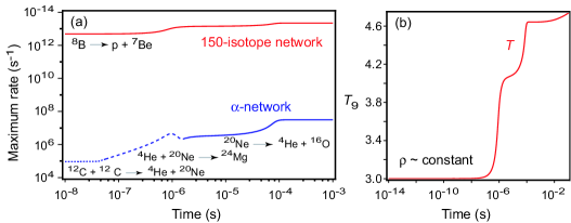
Figure 12: (a) Maximum rates as a function of time in an alpha network and a 150-isotope network for constant density and a hydrodynamic temperature profile given in part (b). Rates were computed using the compilation in Ref. [12]. (b) Hydrodynamical temperature profile corresponding to the calculation shown in part (a); the density is approximately constant over this time range. This profile is characteristic of evolution under Type Ia supernova conditions in a single zone of a carbon–oxygen white dwarf with an initial $T_{9}=3$ and $\rho=1\times 10^{7}\mbox{\ g\,cm}^{-3}$.

The fastest rates in the realistic network are seen to be 6–8 orders of magnitude larger than those in the alpha network for this example. These very fast reactions will tend to bring reaction groups into equilibrium rapidly. Thus, we find that realistic networks are much stiffer than alpha networks, but the most important effect for an explicit integration is not the increased magnitude of the stiffness itself (which the asymptotic and QSS approximations can handle in a manner competitive with implicit methods, as documented in Refs. [1, 2]), but rather that these fast reactions quickly manifest themselves in fast equilibration timescales, which asymptotic and QSS algorithms cannot deal effectively with unless supplemented by a partial equilibrium approximation.

In Fig. 13

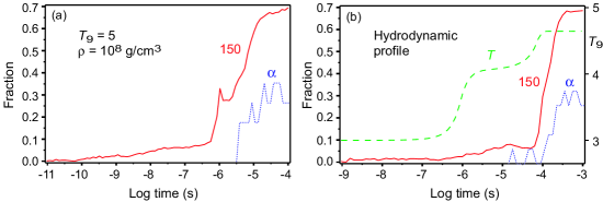
Figure 13: Fraction of equilibrated reactions as a function of time for an alpha network (dotted blue, labeled $\alpha$) and a 150-isotope network (solid red, labeled 150). (a) Constant temperature $T_{9}=5$ and constant density $\rho=10^{8}\mbox{\ g\,cm}^{-3}$ case. (b) Case with hydrodynamic profile having density essentially constant and the temperature variation given by the dashed green line, with $T_{9}$ indicated on the right axis. In both cases we see that the 150-isotope network equilibrates much faster and much more extensively than the alpha network. In these examples we have assumed a reaction group to be in equilibrium if all isotopes participating in the reactions of the group have abundances $Y_{i}$ within 1% of their equilibrium values.

we compare how quickly reactions come into equilibrium (a) for an alpha network and for a 150-isotope network under constant temperature and density conditions typical of some zones in a Type Ia supernova explosion, and (b) using a hydrodynamical profile derived from one zone of a Type Ia supernova simulation. In this calculation we have not yet implemented the partial equilibrium approximation, but have integrated using the asymptotic approximation and tracked the number of reactions that would satisfy the partial equilibrium condition as a function of time in that case. We see that the effect is quite pronounced, with the large, realistic network having a much greater fraction of its reactions satisfying the partial equilibrium condition from very early times when compared with the alpha network. For example, by the time the alpha network begins to show any substantial equilibration the 150-isotope network is 30–40% equilibrated in both cases. This suggests that the partial equilibrium approximation may have an even more dramatic effect on the speed with which large networks can be integrated than we have found for alpha networks.

11.2 A Toy Model: Protons Plus Alpha-Particles

Let us illustrate the ideas of the previous section with a toy model that is simple to understand, but that contains many of the essential features expected for a realistic network. In Fig. 14

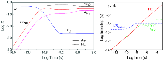
Figure 14: 4-isotope alpha network for constant temperature $T_{9}=5$ and density $\rho=1\times 10^{8}\mbox{\ g\,cm}^{-3}$. Reactions rates were taken from Ref. [12] and initially there were equal mass fractions of ¹²C and ¹⁶O. (a) Mass fractions (asymptotic solid; asymptotic plus partial equilibrium dotted). (b) Timestepping (solid red for asymptotic plus partial equilibrium and dotted green for asymptotic). The maximum stable purely-explicit timestep is estimated by $1/R_{\mbox{\scriptsize max}}$ and shown as the dashed blue curve.

we display a calculation with a 4-isotope alpha network containing the isotopes ⁴He, ¹²C, ¹⁶O, and ²⁰Ne, including all reactions among these species from the REACLIB [12] library. We see that the partial equilibrium abundances are essentially identical to those calculated using only the explicit asymptotic algorithm, and that at the end of the calculation the partial equilibrium calculation is taking timesteps that are about 3 orders of magnitude larger than those for the explicit asymptotic method alone, and about 4 orders of magnitude larger than the maximum timestep that would be stable for a standard explicit method.

In Fig. 15

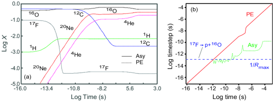
Figure 15: 4-isotope alpha network plus protons and ¹⁷F, for constant temperature $T_{9}=5$ and density $\rho=1\times 10^{8}\mbox{\ g\,cm}^{-3}$. Reactions rates were taken from Ref. [12] and the initial mass fractions were $X_{0}(\mbox{${}^{12}$C},\mbox{${}^{16}$O},\mbox{${}^{1}$H},\mbox{${}^{17}$F})=(0.500,\,0.400,\,0.001,0.122)$. (a) Mass fractions (asymptotic solid; asymptotic plus partial equilibrium dotted). (b) Timestepping (solid red for asymptotic plus partial equilibrium and dotted green for asymptotic). The maximum stable purely-explicit timestep is estimated by $1/R_{\mbox{\scriptsize max}}$ and shown as the dashed blue line. It is determined by the rate for $\mbox{${}^{17}$F}\rightarrow p+\mbox{${}^{16}$O}$ across the entire time range shown. This photodisintegration rate is constant because the temperature is constant.

we repeat the calculation of Fig. 14, except that we add to the 4-isotope alpha network two new isotopes: protons and ¹⁷F. Now the network contains new reactions involving protons that are much faster than the alpha reactions and hence is much stiffer. Again we find that the mass fractions calculated using the asymptotic plus partial equilibrium method and the asymptotic method alone are almost identical, but the disparity in the corresponding integration speeds is now much larger. At the end of the calculation illustrated in Fig. 15, we see that the PE integrator is taking timesteps that are about $10^{6}$ times larger than those for the explicit asymptotic integrator, and almost $10^{9}$ times larger than would be stable with a normal explicit method without the partial equilibrium approximation.

This simple example illustrates succinctly the arguments of the previous section. Comparing Fig. 15 with Fig. 14, we see that the addition of a single set of proton reactions has an enormous influence on the stiffness of the network. In the pure $\alpha$-particle case of Fig. 14, the maximum stable fully-explicit timestep in the approach to equilibrium is of order $10^{-8}\mbox{\ s}$ and is set by $\alpha$-particle reactions. In this case a sufficient number of isotopes become asymptotic to permit an asymptotic timestep of near $10^{-7}$ seconds in the approach to equilibrium. This is not a competitive timestep, since we see from Fig. 14 that the PE method is able to take timesteps about three orders of magnitude larger, but it is far better than the situation in Fig. 15. There we see that the maximum stable fully-explicit timestep over the entire range of integration is of order only $10^{-13}\mbox{\ s}$, because it is set by proton reactions that are much faster than any $\alpha$-particle reaction, as we have already illustrated in Fig. 12. (Under these conditions the fastest of these is the photodisintegration $\gamma+\mbox{${}^{17}$F}\rightarrow p+\mbox{${}^{16}$O}$.)

In Fig. 15 the PE method is taking timesteps in the approach to equilibrium that are six orders of magnitude larger than those of the pure asymptotic method. The reason for this increased disparity between the PE plus asymptotic and pure asymptotic methods is not primarily a better timestep for the PE method (it is taking timesteps in both calculations that are near the limit imposed by accuracy constraints), but rather the large depression of the maximum stable asymptotic timestep produced by adding the much faster proton reactions to the network. However, we see that when the fast proton reactions are removed from the numerical integration by the PE approximation, the timestep of Fig. 15 becomes comparable to that for the much less stiff pure alpha network of Fig. 14.

Hence, our toy model supports rather well the speculations of the previous section. Realistic large networks are much stiffer than $\alpha$-networks, but this increased stiffness is associated largely with fast neutron and proton reactions that may be more susceptible to improvement by partial equilibrium approximations than simple alpha networks. The results of this section suggest that in large realistic networks the systematic removal of the fastest timescales by the PE approximation may permit timestepping by these explicit methods that is comparable to that of implicit methods, even when equilibrium is important. As we have seen, timestepping comparable to that of implicit methods in large networks implies that an explicit partial equilibrium code should be considerably faster than the implicit code, because it can compute each timestep faster.

12 Summary and Conclusions

Numerical integration for extremely stiff reaction networks has typically been viewed as requiring implicit schemes, because normally explicit timesteps of efficient size would be unstable. An alternative to implicit integration modifies the equations using approximate solutions to reduce the stiffness, and then integrates the resulting equations explicitly. For example, asymptotic and quasi-steady-state methods found a measure of success integrating moderately stiff chemical-kinetics systems explicitly [3, 18, 10], but have generally failed for extremely stiff systems, giving inaccurate results with non-competitive integration timesteps. In this paper, and the two preceding it [1, 2], we have presented evidence suggesting that algebraically-stabilized explicit integration can give correct results and timesteps competitive with that of implicit methods for even the stiffest of networks.

Central to this new view of the efficacy of explicit integration for stiff systems is the understanding that in reaction networks there are at least three different sources of stiffness:

1. Negative populations, which can occur for an initially small positive population if an explicit timestep is too large; this anomalous negative population leads to exponentially growing terms that destabilize the network.

2. Macroscopic equilibration, where the right sides of the differential equations $dY=F=F^{+}-F^{-}$ approach a constant derived from the difference of two large numbers (the total flux in $F^{+}$ and total flux out $F^{-}$), and numerical errors in taking this difference destabilize the network if the timestep is too large.

3. Microscopic equilibration, where on the right sides of Eq. (1) the net flux in specific forward-reverse reaction pairs $(f^{+}_{i}-f^{-}_{i})$ tends to zero as the system approaches equilibrium; this leads to large errors if the timestep is too large because the net flux is derived from the difference of two large numbers and the timescale equilibrating the populations is short compared with the desired numerical timestep.

The algebra required to stabilize the explicit solution depends on which of these forms of stiffness is operative. In Refs. [1, 2] we have shown that asymptotic and quasi-steady-state approximations give correct results, with timestepping highly competitive with implicit methods even for the stiffest of thermonuclear networks, as long as the system exhibits only the first two types of stiffness listed above. However, in those papers we have also shown that asymptotic and quasi-steady-state methods give correct results, but with timesteps that are much larger than for purely explicit methods but still far from competitive with implicit methods, if there is any significant microscopic equilibration in the system.

In this paper we have addressed in depth the role of microscopic equilibration in stiffness and presented a partial equilibrium scheme that can be used to augment asymptotic and quasi-steady-state methods when equilibrium becomes important in a network. We have presented strong evidence that this partial equilibrium scheme can remove the timestepping deficiencies encountered by asymptotic and quasi-steady-state methods in the approach to equilibrium, making these methods competitive with implicit methods even near equilibrium. The methods that we have presented build on earlier work [3, 18, 10], but we find that our versions of asymptotic and quasi-steady-state methods are far more accurate, and our versions of partial equilibrium are faster by multiple orders of magnitude, than found in previous work when applied to extremely stiff astrophysical thermonuclear networks.

The present paper, in conjunction with the previous ones on asymptotic methods [1] and quasi-steady-state methods [2], suggests that algebraically-stabilized explicit integration methods are capable of stable timesteps competitive with those of implicit methods even for extremely-stiff reaction networks. Explicit methods can compute timesteps faster than implicit methods in large networks, implying that algebraically-stabilized explicit algorithms may compete favorably with implicit integration, even in complex, extremely-stiff applications. Because explicit methods scale linearly with network size, these findings could permit the coupling of physically more realistic reaction networks to fluid dynamics simulations in a variety of fields.

Appendix A Appendix: Reaction Group Classification

Applying the principles discussed §4.5 to the reaction group classes in Table 2 gives the following systematic partial equilibrium properties of reaction group classes for astrophysical thermonuclear networks.

Reaction Group Class A (a $\rightleftharpoons$ b)

Source term: $\frac{dy_{a}}{dt}=-k_{\mbox{\scriptsize f}}y_{a}+k_{\mbox{\scriptsize r}}y_{b}\quad$ Constraints: $y_{a}+y_{b}\equiv c_{1}=y_{a}^{0}+y_{b}^{0}$

Equation: $\frac{dy_{a}}{dt}=by_{a}+c\quad b=-k_{\mbox{\scriptsize f}}\quad c=k_{\mbox{\scriptsize r}}\quad$ Solution: $y_{a}(t)=y_{a}^{0}e^{bt}-\frac{c}{b}\left(1-e^{bt}\right)$

Equil. solution: $\bar{y}_{a}=-\frac{c}{b}=\frac{k_{\mbox{\scriptsize r}}}{k_{\mbox{\scriptsize f}}}\quad$ Equil. timescale: $\tau=\frac{1}{b}=\frac{1}{k_{\mbox{\scriptsize f}}}$

Equil. tests: $\frac{|y_{i}-\bar{y}_{i}|}{\bar{y}_{i}}<\epsilon_{i}\ \ (i=a,b)\quad$ Equil. constraint: $\frac{y_{a}}{y_{b}}=\frac{k_{\mbox{\scriptsize r}}}{k_{\mbox{\scriptsize f}}}$

Other variables: $y_{b}=c_{1}-y_{a}$

Progress variable: $\lambda\equiv y_{a}^{0}-y_{a}\quad y_{a}=y_{a}^{0}-\lambda\quad y_{b}=y_{b}^{0}+\lambda$

Reaction Group Class B (a + b $\rightleftharpoons$ c)

Source term: $\frac{dy_{a}}{dt}=-k_{\mbox{\scriptsize f}}y_{a}y_{b}+k_{\mbox{\scriptsize r}}y_{c}$

Constraints: $y_{b}-y_{a}\equiv c_{1}=y_{b}^{0}-y_{a}^{0}\quad$ $y_{b}+y_{c}\equiv c_{2}=y_{b}^{0}+y_{c}^{0}$

Equation: $\frac{dy_{a}}{dt}=ay_{a}^{2}+by_{a}+c\quad$ $a=-k_{\mbox{\scriptsize f}}\quad b=-(c_{1}k_{\mbox{\scriptsize f}}+k_{b})\quad c=k_{\mbox{\scriptsize r}}(c_{2}-c_{1})$

Solution: Eq. (19)     Equil. solution: Eq. (21)     Equil. timescale: Eq. (23)

Equil. tests: $\frac{|y_{i}-\bar{y}_{i}|}{\bar{y}_{i}}<\epsilon_{i}\ \ (i=a,b,c)\quad$ Equil. constraint: $\frac{y_{a}y_{b}}{y_{c}}=\frac{k_{\mbox{\scriptsize r}}}{k_{\mbox{\scriptsize f}}}$

Other variables: $y_{b}=c_{1}+y_{a}\quad y_{c}=c_{2}-y_{b}$

Progress variable: $\lambda\equiv y_{a}^{0}-y_{a}\quad y_{a}=y_{a}^{0}-\lambda\quad y_{b}=y_{b}^{0}-\lambda\quad$ $y_{c}=y_{c}^{0}+\lambda$

Reaction Group Class C (a + b + c $\rightleftharpoons$ d)

Source term: $\frac{dy_{a}}{dt}=-k_{\mbox{\scriptsize f}}y_{a}y_{b}y_{c}+k_{\mbox{\scriptsize r}}y_{d}\quad$ Constraints: $y_{a}-y_{b}\equiv c_{1}=y_{a}^{0}-y_{b}^{0}$

$\mbox{$\small\frac{1}{3}$}(y_{a}+y_{b}+y_{c})+y_{d}\equiv c_{3}=\mbox{$\small\frac{1}{3}$}(y_{a}^{0}+y_{b}^{0}+y_{c}^{0})+y_{d}^{0}\quad$ $y_{a}-y_{c}\equiv c_{2}=y_{a}^{0}-y_{c}^{0}$

Equation: $\frac{dy_{a}}{dt}=ay_{a}^{2}+by_{a}+c$

$a=-k_{\mbox{\scriptsize f}}y_{a}^{0}+k_{\mbox{\scriptsize f}}(c_{1}+c_{2})\quad b=-(k_{\mbox{\scriptsize f}}c_{1}c_{2}+k_{\mbox{\scriptsize r}})\quad$ $c=(c_{3}+\mbox{$\small\frac{1}{3}$}c_{1}+\mbox{$\small\frac{1}{3}$}c_{2})k_{\mbox{\scriptsize r}}$

Solution: Eq. (19)     Equil. solution: Eq. (21)     Equil. timescale: Eq. (23)

Equil. tests: $\frac{|y_{i}-\bar{y}_{i}|}{\bar{y}_{i}}<\epsilon_{i}\ \ (i=a,b,c,d)$     Equil. constraint: $\frac{y_{a}y_{b}y_{c}}{y_{d}}=\frac{k_{\mbox{\scriptsize r}}}{k_{\mbox{\scriptsize f}}}$

Other variables: $y_{b}=y_{a}-c_{1}\quad y_{c}=y_{a}-c_{2}$     $y_{d}=c_{3}-y_{a}+\mbox{$\small\frac{1}{3}$}(c_{1}+c_{2})$

Progress variable: $\lambda\equiv y_{a}^{0}-y_{a}\quad y_{a}=y_{a}^{0}-\lambda$     $y_{b}=y_{b}^{0}-\lambda$     $y_{c}=y_{c}^{0}-\lambda$

$y_{d}=\lambda+y_{d}^{0}$

Reaction Group Class D (a + b $\rightleftharpoons$ c + d)

Source term: $\frac{dy_{a}}{dt}=-k_{\mbox{\scriptsize f}}y_{a}y_{b}+k_{\mbox{\scriptsize r}}y_{c}y_{d}\quad$ Constraints: $y_{a}-y_{b}\equiv c_{1}=y_{a}^{0}-y_{b}^{0}$

$y_{a}+y_{c}\equiv c_{2}=y_{a}^{0}+y_{c}^{0}$     $y_{a}+y_{d}\equiv c_{3}=y_{a}^{0}+y_{d}^{0}$

Equation: $\frac{dy_{a}}{dt}=ay_{a}^{2}+by_{a}+c$     $a=k_{\mbox{\scriptsize r}}-k_{\mbox{\scriptsize f}}\quad b=-k_{\mbox{\scriptsize r}}(c_{2}+c_{3})+k_{\mbox{\scriptsize f}}c_{1}\quad c=k_{\mbox{\scriptsize r}}c_{2}c_{3}$

Solution: Eq. (19)     Equil. solution: Eq. (21)     Equil. timescale: Eq. (23)

Equil. tests: $\frac{|y_{i}-\bar{y}_{i}|}{\bar{y}_{i}}<\epsilon_{i}\ \ (i=a,b,c,d)$     Equil. constraint: $\frac{y_{a}y_{b}}{y_{c}y_{d}}=\frac{k_{\mbox{\scriptsize r}}}{k_{\mbox{\scriptsize f}}}$

Other variables: $y_{b}=y_{a}-c_{1}\quad y_{c}=c_{2}-y_{a}\quad y_{d}=c_{3}-y_{a}$

Progress variable: $\lambda\equiv y_{a}^{0}-y_{a}\quad y_{a}=y_{a}^{0}-\lambda\quad y_{b}=y_{b}^{0}-\lambda$ $y_{c}=y_{c}^{0}+\lambda$

$y_{d}=y_{d}^{0}+\lambda$

Reaction Group Class E (a + b $\rightleftharpoons$ c + d + e)

Source term: $\frac{dy_{a}}{dt}=-k_{\mbox{\scriptsize f}}y_{a}y_{b}+k_{\mbox{\scriptsize r}}y_{c}y_{d}y_{e}$

Constraints: $y_{a}+\mbox{$\small\frac{1}{3}$}(y_{c}+y_{d}+y_{e})\equiv c_{1}=y_{a}^{0}+\mbox{$\small\frac{1}{3}$}(y_{c}^{0}+y_{d}^{0}+y_{e}^{0})$

$y_{a}-y_{b}\equiv c_{2}=y_{a}^{0}-y_{b}^{0}\quad y_{c}-y_{d}\equiv c_{3}=y_{c}^{0}-y_{d}^{0}$     $y_{c}-y_{e}\equiv c_{4}=y_{c}^{0}-y_{e}^{0}$

Equation: $\frac{dy_{a}}{dt}=ay_{a}^{2}+by_{a}+c$

$a=(3c_{1}-y_{a}^{0})k_{\mbox{\scriptsize r}}-k_{\mbox{\scriptsize f}}\quad b=c_{2}k_{\mbox{\scriptsize f}}-(\alpha\beta+\alpha\gamma+\beta\gamma)k_{\mbox{\scriptsize r}}$     $c=k_{\mbox{\scriptsize r}}\alpha\beta\gamma$

$\alpha\equiv c_{1}+\mbox{$\small\frac{1}{3}$}(c_{3}+c_{4})\quad\beta\equiv c_{1}-\mbox{$\small\frac{2}{3}$}c_{3}+\mbox{$\small\frac{1}{3}$}c_{4}$     $\gamma\equiv c_{1}+\mbox{$\small\frac{1}{3}$}c_{3}-\mbox{$\small\frac{2}{3}$}c_{4}$

Solution: Eq. (19)     Equil. solution: Eq. (21)     Equil. timescale: Eq. (23)

Equil. tests: $\frac{|y_{i}-\bar{y}_{i}|}{\bar{y}_{i}}<\epsilon_{i}\ \ (i=a,b,c,d,e)$     Equil. constraint: $\frac{y_{a}y_{b}}{y_{c}y_{d}y_{e}}=\frac{k_{\mbox{\scriptsize r}}}{k_{\mbox{\scriptsize f}}}$

Other variables: $y_{b}=y_{a}-c_{2}\quad y_{c}=\alpha-y_{a}\quad y_{d}=\beta-y_{a}$     $y_{e}=\gamma-y_{a}$

Progress variable: $\lambda\equiv y_{a}^{0}-y_{a}\quad y_{a}=y_{a}^{0}-\lambda\quad y_{b}=y_{b}^{0}-\lambda\quad$ $y_{c}=y_{c}^{0}+\lambda$

$y_{d}=y_{d}^{0}+\lambda\quad y_{e}=y_{e}^{0}+\lambda$

In the equilibrium tests we have allowed the possibility of a different $\epsilon_{i}$ for each species $i$, but in practice one would often choose the same small value $\epsilon$ for all $i$. The results presented in this paper typically have used $\epsilon_{i}=0.01$ for all species.

References

- [1] Guidry M W, Budiardja R, Feger E, Billings J J, Hix W R, Messer O E B, Roche K J, McMahon E and He M 2011 Explicit Integration of Extremely-Stiff Reaction Networks: Asymptotic Methods (arXiv:1112.4716)
- [2] Guidry M W and Harris J A 2011 Explicit Integration of Extremely-Stiff Reaction Networks: Quasi-Steady-State Methods (arXiv:1112.4750)
- [3] Oran E S and Boris J P 2005 Numerical Simulation of Reactive Flow (Cambridge: Cambridge University Press)
- [4] Arvidson R S, Mackenzie F T and Guidry M 2006 MAGic: A Phanerozoic Model for the Geochemical Cycling of Major Rock-Forming Components American Journal of Science 306 135-90
- [5] Hix W R and Meyer B S 2006 Thermonuclear kinetics in astrophysics Nuc. Phys. A 777 188-207
- [6] Timmes F X 1999 Integration of Nuclear Reaction Networks for Stellar Hydrodynamics Astrophys. J. Suppl. 124 241-63
- [7] Gear C W 1971 Numerical Initial Value Problems in Ordinary Differential Equations (Englewood Cliffs, NJ: Prentice Hall)
- [8] Lambert J D 1991 Numerical Methods for Ordinary Differential Equations (New York: Wiley)
- [9] Press W H, Teukolsky S A, Vettering W T and Flannery B P 1992 Numerical Recipes in Fortran (Cambridge: Cambridge University Press)
- [10] Mott D R 1999 New Quasi-Steady-State and Partial-Equilibrium Methods for Integrating Chemically Reacting Systems PhD thesis University of Michigan at Ann Arbor
- [11] Feger E 2011 Evaluating Explicit Methods for Solving Astrophysical Nuclear Reaction Networks PhD thesis University of Tennessee at Knoxville
- [12] Rauscher T and Thielemann F-K 2000 Astrophysical Reaction Rates From Statistical Model Calculations At. Data Nuclear Data Tables 75 1-351
- [13] Guidry M W 2011 Algebraic Stabilization of Explicit Numerical Integration for Extremely Stiff Reaction Networks (arXiv:1112.4778)
- [14] Cyburt R H et al 2010 The JINA REACLIB Database: Its Recent Updates and Impact on Type-I X-ray Bursts Astrophys. J. Suppl. 189 240-52 http://groups.nscl.msu.edu/jina/reaclib/db/
- [15] Hix W R and Thielemann F-K 1999 Computational methods for nucleosynthesis and nuclear energy generation J. Comp. Appl. Mathematics 109 321-51
- [16] Khokhlov A YASS - yet another stiff solver that works NRL Technical Memorandum Report
- [17] Bronson Messer, private communication; Timmes F X, Hoffman R D, and Woosley S E 2000 An inexpensive nuclear energy generation network for stellar hydrodynamics ApJS 129 377-398
- [18] Mott D R, Oran E S and van Leer B 2000 Differential Equations of Reaction Kinetics J. Comp. Phys. 164 407-28