Impact of supernova dynamics on the $\nu p$-process

Abstract

We study the impact of the late time dynamical evolution of ejecta from core-collapse supernovae on $\nu p$-process nucleosynthesis. Our results are based on hydrodynamical simulations of neutrino wind ejecta. Motivated by recent two-dimensional wind simulations, we vary the dynamical evolution during the $\nu p$-process and show that final abundances strongly depend on the temperature evolution. When the expansion is very fast, there is not enough time for antineutrino absorption on protons to produce enough neutrons to overcome the $\beta^{+}$-decay waiting points and no heavy elements beyond $A=64$ are produced. The wind termination shock or reverse shock dramatically reduces the expansion speed of the ejecta. This extends the period during which matter remains at relatively high temperatures and is exposed to high neutrino fluxes, thus allowing for further $(p,\gamma)$ and $(n,p)$ reactions to occur and to synthesize elements beyond iron. We find that the $\nu p$-process starts to efficiently produce heavy elements only when the temperature drops below $\sim 3$ GK. At higher temperatures, due to the low alpha separation energy of ⁶⁰Zn ($S_{\alpha}=2.7$ MeV) the reaction ⁵⁹Cu$(p,\alpha)$⁵⁶Ni is faster than the reaction ⁵⁹Cu$(p,\gamma)$⁶⁰Zn. This results in the closed NiCu cycle that we identify and discuss here for the first time. We also investigate the late phase of the $\nu p$-process when the temperatures become too low to maintain proton captures. Depending on the late neutron density, the evolution to stability is dominated by $\beta^{+}$ decays or by $(n,\gamma)$ reactions. In the latter case, the matter flow can even reach the neutron-rich side of stability and the isotopic composition of a given element is then dominated by neutron-rich isotopes.

1 Introduction

Neutrino-driven winds from core-collapse supernova explosions contribute to the synthesis of elements beyond iron. After the explosion, the hot proto-neutron star cools emitting neutrinos. These neutrinos interact with the stellar matter and deposit energy in the outer layers of the proto-neutron star leading to a supersonic outflow known as neutrino-driven wind Duncan et al. (1986). Although neutrino-driven winds were considered the site where heavy elements are produced by the r-process Woosley et al. (1994), recent simulations Arcones et al. (2007); Hüdepohl et al. (2010); Fischer et al. (2010); Roberts et al. (2010) cannot reproduce the extreme conditions required for producing heavy r-process elements (see e.g., Hoffman et al., 1997; Otsuki et al., 2000; Thompson et al., 2001). The wind entropy is too low (less than $100\,k_{\mathrm{B}}/\mathrm{nuc}$) and, even more significant, the ejecta is proton rich (the electron fraction $Y_{e}$ remains above 0.5 during seconds, see Hüdepohl et al. (2010); Fischer et al. (2010)). Even if the r-process does not take place in every neutrino-driven wind, lighter heavy elements (e.g., Sr, Y, Zr) can be synthesized in this environment as suggested by Qian & Wasserburg (2001). In proton-rich conditions Fröhlich et al. (2006) showed that elements beyond ⁶⁴Ge can be synthesized. Wanajo et al. (2011b) found Sr, Y, Zr in small pockets of neutron rich material ejected after the explosion of low mass progenitors. Recently, Arcones & Montes (2011) performed a systematic nucleosynthesis study that strongly supports the production of lighter heavy elements in proton- and neutron-rich neutrino-driven winds.

In proton-rich winds, charged particle reactions (alpha and proton captures) build nuclei up to ⁵⁶Ni and even up to ⁶⁴Ge once the temperature drops below 3 GK. Due to their long beta-decay lifetimes and low thresholds for proton capture, the nuclei ⁵⁶Ni and ⁶⁴Ge act as bottlenecks that inhibit the production of heavier elements. In the $\nu p$-process, their decay is sped up by $(n,p)$ reactions, with the neutrons produced by antineutrino absorption on the abundant free protons. This allows for the production of elements beyond iron and may explain the origin of light p-nuclei Fröhlich et al. (2006); Pruet et al. (2006); Wanajo (2006); Wanajo et al. (2011a). The synthesis of elements by the $\nu p$-process depends thus on neutrino spectra and luminosities but also on the dynamical evolution as matter expands through the slow, early supernova ejecta. This produces a wind termination shock or reverse shock where kinetic energy is transformed into internal energy Arcones et al. (2007). The reverse shock has a big impact on the nucleosynthesis because temperature and density increase and the expansion is strongly decelerated. This hydrodynamical feature has been extensively studied for r-process nucleosynthesis Qian & Woosley (1996); Sumiyoshi et al. (2000); Wanajo (2007); Panov & Janka (2009); Arcones & Martínez-Pinedo (2011). Recently, Wanajo et al. (2011a) have also explored the relevance of the reverse shock on the $\nu p$-process. Motivated by their work and by new 2D hydrodynamical simulations of the neutrino-driven wind Arcones & Janka (2011), we investigate here the wind termination shock to gain further insights on the dynamical evolution relevant for the $\nu p$-process.

Here we use a trajectory from hydrodynamical simulations (Sect. 2) combined with a complete nucleosynthesis network (Sect. 3). In Sect. 4 we present our results where we analyze the impact of the wind termination temperature (Sect. 4.1), the temperature jump at the reverse shock (Sect. 4.2), and the influence of late temperature evolution and the decay to stability (Sect 4.3). Our conclusions are summarized in Sect. 5.

2 Long-time dynamical evolution

Our study is based on one trajectory obtained from hydrodynamical simulations by Arcones et al. (2007). These simulations follow the supernova explosion and the subsequent neutrino-driven wind.

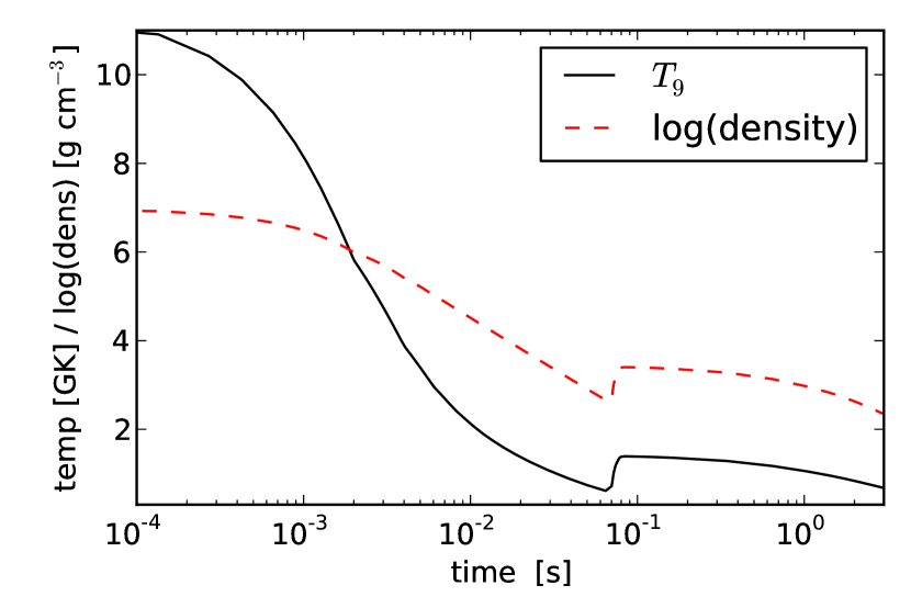
Figure 1: Evolution of density and temperature along a trajectory ejected at 2s after bounce of model M15l1r1 in Arcones et al. (2007). The reverse shock is at $T_{\mathrm{wt}}\approx 0.6$ GK and produces a jump in density and temperature and a sudden decrease of the expansion velocity.

Figure 1 presents the evolution of density and temperature for the chosen trajectory. In the following, we always use the same initial evolution and modify it at temperatures below 3 GK. We assume the wind terminates at a temperature $T_{\mathrm{wt}}$ and the evolution thereafter is varied using the prescription introduced by Arcones & Martínez-Pinedo (2011) and motivated by 1D and 2D hydrodynamical simulations Arcones et al. (2007); Arcones & Janka (2011). The thermodynamical conditions at the termination of the wind depend on both the intrinsic properties of the wind, like its velocity and mass outflow rate, and on the pressure of the slow moving ejecta. The wind properties are determined by the neutrino energies and luminosities and by the neutron star mass and radius (see e.g., Qian & Woosley, 1996). These conditions depend mainly on the nuclear equation of state and are similar for different progenitors Arcones et al. (2007); Fischer et al. (2010). The properties of the slow supernova ejecta are related to the progenitor and become very anisotropic during the evolution Arcones & Janka (2011).

In our calculations, we use a simple model that reproduces the main features seen in hydrodynamical simulations. Once the wind reaches the early supernova ejecta we use the Rankine-Hugoniot conditions to determine the behavior of temperature, density, and velocity. When the wind moves supersonically these quantities jump at the reverse shock. The evolution after such discontinuity is determined assuming constant density and temperature during a time $\Delta t$. As the mass outflow is constant ($\dot{M}=4\pi r^{2}v\rho$) the velocity drops as $v\propto r^{-2}$. At later times, the velocity stays constant and the density decreases as $\rho\propto r^{-2}$ (see Arcones & Martínez-Pinedo (2011) for more details). To account for the differences found in the late evolution in two-dimensional simulations, we will use different values of $\Delta t$ and explore the impact on the nucleosynthesis.

3 Nucleosynthesis network

The evolution of the composition is calculated using a full reaction network Fröhlich et al. (2006). All calculations start when the temperature drops below 10 GK and are followed until the temperature reaches 0.01 GK. We assume the initial composition to be determined from nuclear statistical equilibrium for a fixed electron fraction $Y_{e}=0.52$. The reaction network includes 1869 nuclei from free nucleons to dysprosium ($Z=66$). Neutral and charged particle reactions are taken from the REACLIB compilation, containing theoretical statistical-model rates by Rauscher & Thielemann (2000) (NON-SMOKER) and experimental rates by Angulo et al. (1999). The theoretical weak interactions rates are taken from Langanke & Martínez-Pinedo (2001) and Fuller et al. (1982). Where available, experimental beta-decay rates are used from NuDat2 supplemented by theoretical beta-decay rates Möller et al. (2003). Neutrino absorption on nucleons and nuclei is also taken into account. We assume a constant neutrino luminosity for neutrinos and anti-neutrinos ($L_{\nu_{e}}=L_{\bar{\nu}_{e}}=5\times 10^{51}$ erg), and Fermi-Dirac spectra with a temperature consistent with the hydrodynamical simulations.

In order to understand the nucleosynthesis evolution, it is useful to look at the time variations of the mean lifetimes for $\beta^{+}$-decays, $(n,\gamma)$, $(p,\gamma)$, $(n,p)$, $(\gamma,n)$, and $(\gamma,p)$ reactions. These mean lifetimes (or average timescales) are defined as

$$\tau_{\beta^{+}}\equiv\left[\frac{1}{Y_{h}}\sum_{Z>2,A}\lambda_{\beta^{+}}(Z,A)Y(Z,A)\right]^{-1},$$ (1)

$$\tau_{n\gamma}\equiv\left[\frac{\rho Y_{n}}{Y_{h}}N_{A}\sum_{Z>2,A}\langle\sigma v\rangle_{(n,\gamma)}(Z,A)Y(Z,A)\right]^{-1},$$ (2)

$$\tau_{p\gamma}\equiv\left[\frac{\rho Y_{p}}{Y_{h}}N_{A}\sum_{Z>2,A}\langle\sigma v\rangle_{(p,\gamma)}(Z,A)Y(Z,A)\right]^{-1},$$ (3)

$$\tau_{np}\equiv\left[\frac{\rho Y_{n}}{Y_{h}}N_{A}\sum_{Z>2,A}\langle\sigma v\rangle_{(n,p)}(Z,A)Y(Z,A)\right]^{-1},$$ (4)

$$\tau_{\gamma n}\equiv\left[\frac{1}{Y_{h}}\sum_{Z>2,A}\lambda_{\gamma n}(Z,A)Y(Z,A)\right]^{-1},$$ (5)

and

$$\tau_{\gamma p}\equiv\left[\frac{1}{Y_{h}}\sum_{Z>2,A}\lambda_{\gamma p}(Z,A)Y(Z,A)\right]^{-1},$$ (6)

where $\lambda_{\beta^{+}}(Z,A)$ denotes the decay rate of nucleus $(Z,A)$, $\langle\sigma v\rangle_{x}(Z,A)$ the reaction rate for process $x$ on nucleus $(Z,A)$, and $\lambda_{\gamma n}(Z,A)$, and $\lambda_{\gamma p}(Z,A)$ the photo-dissociation reaction rates with emission of neutron and proton, respectively. In these equations, $N_{A}$ is Avogadro number. The average is taken over the heavy nuclei ($Z>2$):

$$Y_{h}=\sum_{Z>2,A}Y(Z,A).$$ (7)

Another useful quantity to understand the nucleosynthesis evolution is the reaction flow between two nuclei $i$ and $j$ defined as

$$F_{ij}\equiv\dot{Y}(i\rightarrow j)-\dot{Y}(j\rightarrow i)\,.$$ (8)

The quantity $\dot{Y}(i\rightarrow j)$ denotes the change in abundance of nucleus $i$ due to all reactions connecting nucleus $i$ with nucleus $j$. The largest reaction flows at each time step indicate the key reactions and thus the nucleosynthesis path.

4 Results

4.1 Constant temperature

We study here the impact of the wind termination varying the temperature at which it occurs. We assume that the velocity is subsonic and hence there is no jump in temperature, density, and velocity. The different temperature evolutions and their nucleosynthesis are shown in Fig. 2. The original trajectory (solid black line) is also included for completeness and comparison purposes. In the modified trajectories the wind termination is at $T_{\mathrm{wt}}=$ 1, 1.5, 2, 2.5, and 3 GK. The resulting abundances change significantly with temperature $T_{\mathrm{wt}}$. There is an optimal $T_{\mathrm{wt}}$ around $2$ GK for producing heavier elements Wanajo et al. (2011a). Moreover, the nucleosynthesis evolution is very different for temperatures higher and lower than this optimal temperature. This can be seen in Fig. 3 where the relevant averaged timescales (see Sect. 3) are shown for the trajectories with $T_{\mathrm{wt}}=$ 1, 2, 3 GK. Initially, there is $(p,\gamma)-(\gamma,p)$ equilibrium in all cases. The timescales for the $(p,\gamma)$ and $(\gamma,p)$ reactions are much shorter when the wind termination occurs at higher temperatures (see bottom panel of Figure 3).

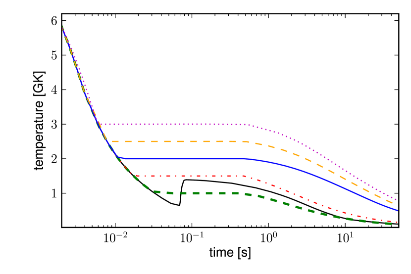
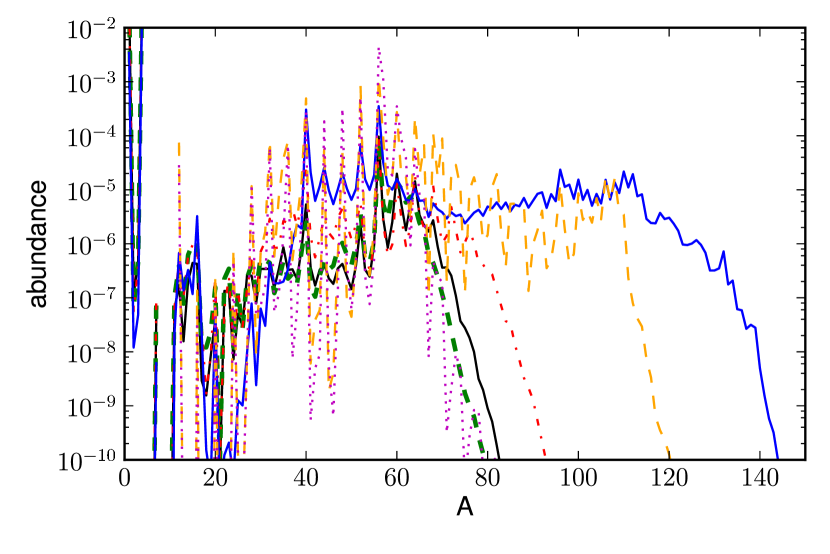
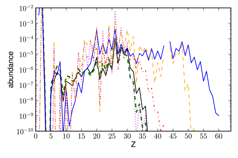
Figure 2: Different temperature evolutions are shown in the upper panel. The solid black line corresponds to the original trajectory. The abundances for these evolutions are presented (with same colors and line styles) in the middle and bottom panels versus mass and proton numbers, respectively.

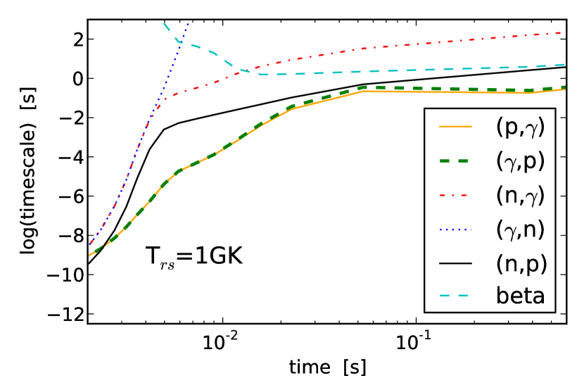
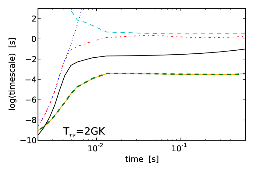
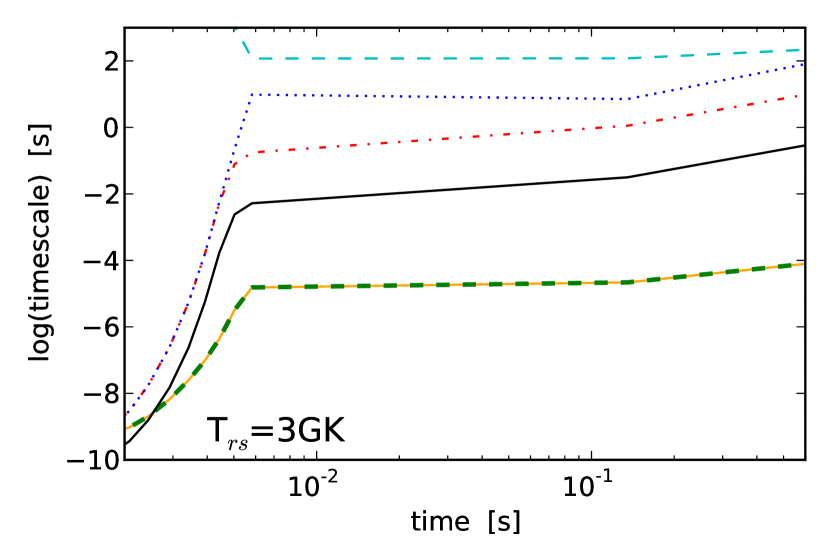
Figure 3: Averaged time scales of the most relevant reactions indicated in the labels. The three panels correspond to the wind termination at 1, 2, and 3 GK from the top to the bottom.

For the wind termination at low temperatures, $T_{\mathrm{wt}}=$ 1, 1.5 GK, only elements up to Germanium are produced in substantial amounts. In these evolutions matter expands very fast. Therefore, it only stays for a short time in the temperature rage of $1.5-3$ GK where charged-particle reactions can effectively synthesize heavier nuclei. In addition, matter rapidly reaches large radii where the antineutrino flux is rather low. Similar conditions are found in explosions of low mass progenitors where the expansion of the supernova ejecta is very fast Hoffman et al. (2008); Wanajo et al. (2009); Roberts et al. (2010); Wanajo et al. (2011a). Notice that the wind termination at a slightly higher temperature, 1.5 GK instead of 1 GK, allows to reach somewhat higher mass number.

For the wind termination at high temperatures, one would expect that photo-dissociation stops the synthesis of heavier elements. In this case, the abundance would continuously shift towards lower mass number as temperature increases. However, in our calculations we see an abrupt change in the abundances when the wind termination temperature exceeds certain value. This points to a key reaction acting as a bottleneck at high temperatures. We have identified such a reaction using the reaction flows introduced in Sect. 3. Figure 4 shows these flows at two different temperatures for the evolution with $T_{\mathrm{wt}}=$ 2 GK. The upper panel corresponds to $T\approx 3.3$ GK, and the bottom one to $T\approx 2.2$ GK, both represent conditions before the constant temperature phase. Notice that the reactions that determine the nucleosynthesis flow are different at high and low temperatures. At high temperatures, the reaction ⁵⁹Cu$(p,\alpha)$⁵⁶Ni dominates over ⁵⁹Cu$(p,\gamma)$⁶⁰Zn while at low temperatures the contrary is true (see Fig. 5). When the ⁵⁹Cu$(p,\alpha)$ reaction dominates, the nucleosynthesis flow is confined into a closed NiCu cycle. A similar behavior has been found in the rp-process for the SnSbTe cycle Schatz et al. (2001).

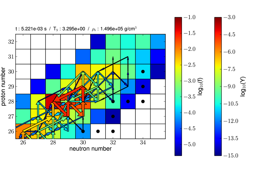
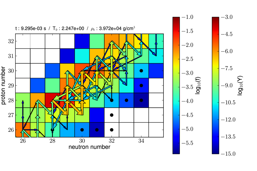
Figure 4: Arrows indicate the flow of different reactions normalized to the strongest one. The colors and sizes of the arrows are proportional to the flow. Abundances are also shown with colors and stable nuclei are indicated with a dot. The upper panel corresponds to the early evolution when the temperature is around 3.3 GK and in the bottom panel it has dropped down to $\sim$ 2.2 GK.

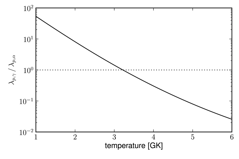
Figure 5: Ratio of proton capture rates on ⁵⁹Cu, with $\lambda_{(p,\gamma)}=\rho Y_{p}N_{A}\langle\sigma v\rangle_{(p,\gamma)}$ and $\lambda_{(p,\alpha)}=\rho Y_{p}N_{A}\langle\sigma v\rangle_{(p,\alpha)}$. At high temperatures ⁵⁹Cu$(p,\alpha)$⁵⁶Ni dominates while for lower temperature ⁵⁹Cu$(p,\gamma)$⁶⁰Zn dominates. Dotted line indicates where rates are equal.

In the calculation with $T_{\mathrm{wt}}=3$ GK, when temperatures are still above $\sim 3.2$ GK (see Fig. 5) the heaviest nucleus produced is ⁵⁶Ni due to the NiCu cycle. Once the temperature drops, the cycle opens and the path reaches ⁶⁴Ge. However, during the high constant temperature phase, the triple alpha reaction maintains a continuous production of seed nuclei from light nuclei with $A\leq 7$ Wanajo et al. (2011a). This leads to a reduction of the proton abundance and thus of the neutrons produced by antineutrino absorption. Notice that the ratio of neutrons produced per seed nucleus is a useful guide of the strength of the $\nu p$-process Pruet et al. (2006). Both effects (the NiCu cycle and the reduced neutron-to-seed ratio) result in a complete shutdown of $\nu p$-process nucleosynthesis.

When the wind termination temperature is very high ($\approx 3$ GK) or very low ($\approx 1$ GK), elements beyond Germanium are hardly synthesized. However, the final abundances are different for these two extreme cases. When the wind termination takes place at high temperatures ($\gtrsim 3$ GK) matter accumulates in iron group nuclei due to the NiCu cycle and to the continuous production of seed nuclei. While for the wind termination at low temperatures matter moves fast to large distances where the antineutrino flux is not large enough to produce a $\nu p$-process. In addition, the low temperatures inhibit the production of seed nuclei. Therefore, the final proton abundance is significantly higher in the evolution with the wind termination at temperatures $\lesssim 2$ GK.

4.2 Reverse shock

When matter moves supersonically there is a jump at the wind termination in temperature and density, also called reverse shock. Here, we analyze the impact of such a jump on the $\nu p$-process nucleosynthesis using the trajectories shown in Fig. 6. The trajectory without jump corresponds to the evolution with $T_{\mathrm{wt}}=2$ GK presented in the previous section. The trajectory with jump is chosen such that the temperature increases after the wind termination reaches $\approx 2$ GK (same temperature as in the trajectory without jump). The constant temperature phase is the same for both evolutions ($\Delta t=0.5$ s). However, the final abundances are very different as shown in Fig. 6.

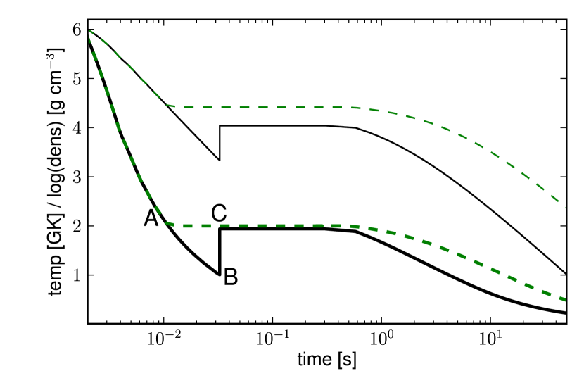
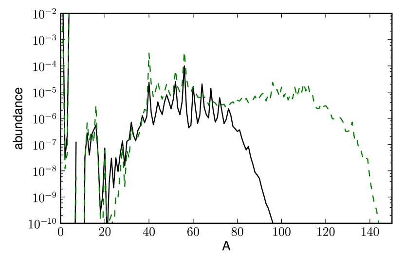
Figure 6: The upper panel shows the temperature (thick lines) and density (thin lines) evolutions with jump (solid black) and without jump (dashed green) at the wind termination. The corresponding abundances vs. mass number are presented in the lower panel.

In the evolution with jump, the expansion continues very fast between the moment the temperature reaches 2 GK (marked with an A in the temperature curve, Fig. 6) and the position of the wind termination shock (marked with B). During this phase, there is not enough time for antineutrino absorption on protons to produce the necessary amount of neutrons to reach heavier nuclei. Already in this phase, between A and B, matter starts to beta decay towards stability because temperatures become too low for proton-capture reactions. The temperature rise at the wind termination, from point B to C, increases the effectiveness of proton-capture reactions. This results in the matter flow moving again away from stability and towards heavier nuclei. Note that the temperature and matter distribution after the wind termination are very similar for both trajectories (points A and C).

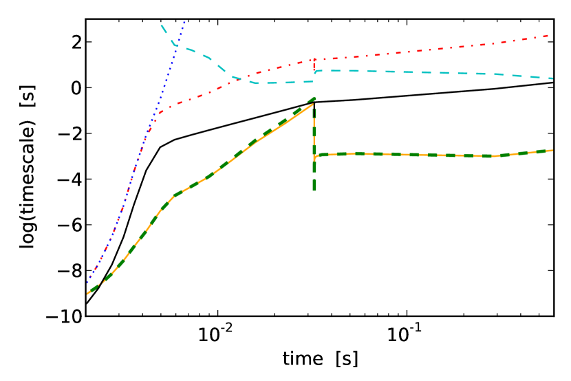
Figure 7: Same as Fig. 3 for the evolution with a jump at the reverse shock.

The relevant timescales for the trajectory with jump are presented in Fig. 7. This can be compared to the middle panel in Fig. 3 that corresponds to the trajectory without jump. After the wind termination, proton-captures are faster for the evolution without jump. More significant are the differences in $(n,\gamma)$ and $(n,p)$ timescales: both are much shorter in the evolution without jump (middle panel in Fig. 3). These differences in the relevant timescales have a big impact on the abundances.

The reactions involving neutrons, i.e., $(n,\gamma)$ and $(n,p)$, depend on the neutron density which is shown in Fig. 8 for the two evolutions. In the trajectory with jump (solid line), the neutron density remains lower than in the trajectory without jump at all times, even at the wind termination (feature at $t\approx 0.02$ s). In the $\nu p$-process there is an equilibrium between neutron capture and neutron production by antineutrino absorption on protons. This implies that

$$\frac{\mathrm{d}Y_{n}}{\mathrm{d}t}=\lambda_{\bar{\nu}_{e}}Y_{p}-\sum_{Z,A}N_{n}Y(Z,A)\langle\sigma v\rangle_{(Z,A)}=0.$$ (9)

Here $\lambda_{\bar{\nu}_{e}}$ is the electron antineutrino absorption rate and $\langle\sigma v\rangle_{(Z,A)}$ is the sum of reaction rates for $(n,\gamma)$ and $(n,p)$ reactions for nucleus (Z, A). Therefore, the neutron density in equilibrium is given by

$$N_{n}=\frac{\lambda_{\bar{\nu}_{e}}Y_{p}}{\sum_{Z,A}Y(Z,A)\langle\sigma v\rangle_{(Z,A)}}.$$ (10)

The nucleosynthesis path is very similar for both trajectories considered here (evolution with and without jump). Therefore, only small variations are expected in the denominator. Consequently, the difference in the neutron densities (see Fig. 8) is due to the neutron production by antineutrinos. The deceleration of the expansion at the wind termination occurs at a smaller radii for the trajectory without jump (see bottom panel of Fig. 8). The production of neutrons is hence less efficient in the case with jump because matter reaches larger radii where the neutrino flux is reduced due to its $r^{-2}$ dependency. The difference in the abundance pattern for nuclei above mass number $A\approx 80$ (see Fig. 6) is due to this difference in the efficiency of neutron production.

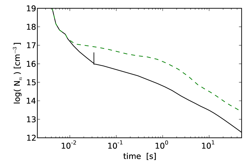
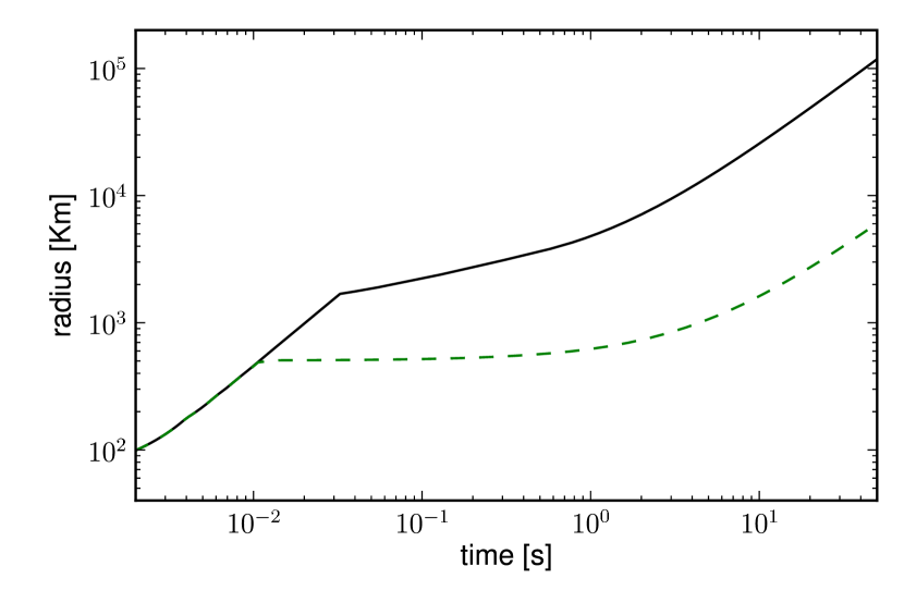
Figure 8: Evolution of neutron density (upper panel) and radius (bottom panel) for the trajectories presented in Fig. 6. The solid black line corresponds to the evolution with jump, the dashed green line to the evolution without jump.

4.3 Late-time evolution

We explore the impact of the dynamical evolution after the wind termination. In this section, we assume that the wind termination occurs at $T_{\mathrm{wt}}=2.0$ GK and we vary the parameter $\Delta t$. The quantity $\Delta t$ characterizes the timescale for the transition from an expansion with constant temperature and density (during which $v\propto r^{-2}$) to a constant velocity expansion with $\rho\propto r^{-2}$. We choose the values $\Delta t=$ 0.0, 0.5, and 1.0 s, motivated by the anisotropic evolution of the ejecta in 2D hydrodynamical simulations Arcones & Janka (2011). There is a smooth transition between the two extreme cases of $\Delta t=1.0$ s and $\Delta t=0.0$ s, which can be seen in the intermediate case of $\Delta t=0.5$ s. The latter ($\Delta t=0.5$ s) was used in previous sections.

The different temperature evolutions (top panel) and the resulting nucleosynthesis (middle and bottom panels) are shown in Fig. 9. While all three cases produce similar abundance distributions, the details depend critically on the value of $\Delta t$.

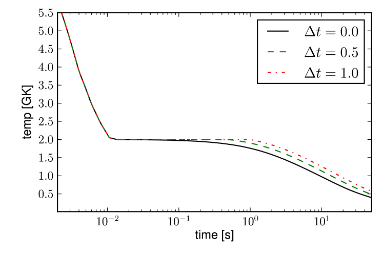
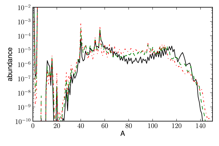
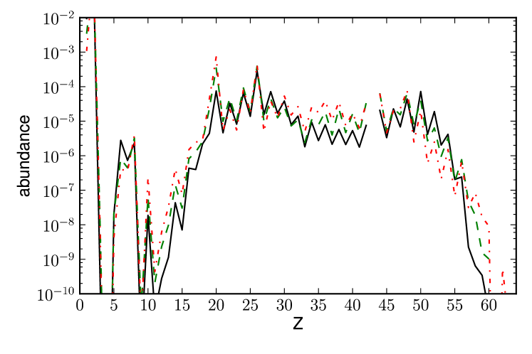
Figure 9: Different temperature evolutions after the wind termination shock which is at 2.0 GK are shown in the top panel. Values for $\Delta t$ are 0.0 s (solid black), 0.5 s (dashed green), and 1.0 s (dotted red). Abundances for these evolutions are shown versus mass number $A$ (middle panel) and versus atomic number $Z$ (bottom panel).

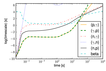
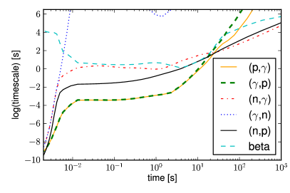
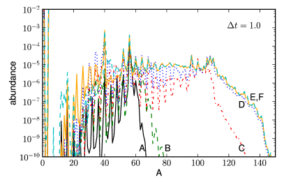
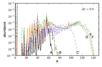
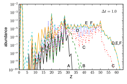
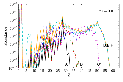
Figure 10: The left column is for the case of $\Delta t=1.0$ s, the right column is for $\Delta t=0.0$ s. The top row shows average timescales for different reaction types as function of time. Abundance distributions at selected times are shown as function of mass number (middle row) and as function of atomic number (bottom row) for both cases of $\Delta t$. For the case $\Delta t=1.0$ s, the abundances are shown at $T=$ 3.0 (A), 2.0 (B,C), 1.6 (D),1.0 GK (E) and also the final abundances (F). The abundances at the beginning (B) and at the end (C) of the constant temperature phase differ quite significantly. For the case $\Delta t=0.0$ s, the abundances are shown at $T=$ 3.0 (A), 2.0 (B), 1.9 (C’), 1.5 (D), 1.0 GK (E) and also the final abundances (F). Note that while the abundances at (C) for $\Delta t=1.0$ s and at (C’) for $\Delta t=0.0$ s are similar, the temperature is slightly lower for (C’) because there is no constant temperature phase in this case.

For a relatively long phase of constant temperature ($\Delta t=1.0$ s; left column of Fig. 10), the $(p,\gamma)-(\gamma,p)$ equilibrium lasts for quite a long time and allows for many $(n,p)$ and $(p,\gamma)$ reactions to occur. This drives the matter to higher mass number (up to $A\approx 110$), where matter accumulates in Sn ($Z=50$ closed shell). Due to the extended period of $(p,\gamma)-(\gamma,p)$ equilibrium, significant abundances of nuclei with $64\lesssim A\lesssim 110$ are synthesized (see line C in Fig. 10 left column). Also during this phase there is a continues production of seed nuclei at the expenses of alpha particle (see Fig.11). Once the temperature drops below $\approx$ 1.5 GK (line D), the production of seed stops. In addition, proton-capture reactions become hindered by the Coulomb barrier and $\beta^{+}$-decays become faster than $(n,p)$ reactions (see upper left panel in Fig 9). The nucleosynthesis ceases to efficiently proceed to higher masses. During this phase, matter starts to decay towards stability. A small number of late time neutron capture reactions smooths the abundance distribution in the mass range $80\lesssim A\lesssim 110$ (line E). Once the temperature drops below 1.0 GK (lines E and F), the abundances as function of mass number do not change anymore, as at this time $\beta^{+}$-decays dominate. The closed shell at $Z=50$ acts as barrier for the nucleosynthesis. This can be seen in the enhanced abundances at $A=110$ (originating from ^110,111,112Sn) in the final abundance distribution.

For the case $\Delta t=0.0$ s (right column in Fig. 10), the situation is very different. The initial phase of $(p,\gamma)-(\gamma,p)$ equilibrium is much shorter than in the case of $\Delta t=1.0$ s. In this case nuclei up to mass number $A\approx 110$ are synthesized (line C’) the temperature has already dropped below 2 GK. Due to the faster temperature decline, the production of seed nuclei is less efficient than in the case of $\Delta t=1.0$ s (see Fig. 11). This leads to lower abundances of nuclei such as ¹²C, ¹⁶O, ²⁰Ne, ²⁸Si, and ⁴⁰Ca for $\Delta t=0$ s (see Fig. 9). The lower abundance of seed nuclei leads to a higher neutron density (see Eq. 10) as in both cases the neutron production rate ( $\lambda_{\bar{\nu}_{e}}Y_{p}$) is similar. Therefore, in the evolution with $\Delta t=0$ s, there are more neutrons available per seed nuclei (Fig. 11). The neutron capture reactions, i.e. $(n,\gamma)$ and $(n,p)$, become faster than $(p,\gamma)$ reactions at temperatures of $T<1.5$ GK. These neutron captures move matter to the neutron-rich side of stability. This, together with the earlier less efficient production of seeds, results in a depletion of the abundances in the region of $64\lesssim A\lesssim 110$ (compare black solid and red dashed line in Fig. 9). Towards the end of the evolution, $(n,\gamma)$ reactions are the fastest ones, even faster than $\beta^{+}$-decays. During this phase, the atomic number $Z$ remains unchanged while the mass number increases (lines D, E, and F in Fig. 10). The signature of matter moving to stability via $(n,\gamma)$ reactions can be seen in the increased abundances at $A=124$, corresponding to ¹²⁴Sn, the most neutron-rich stable Sn isotope.

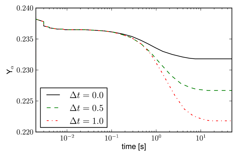
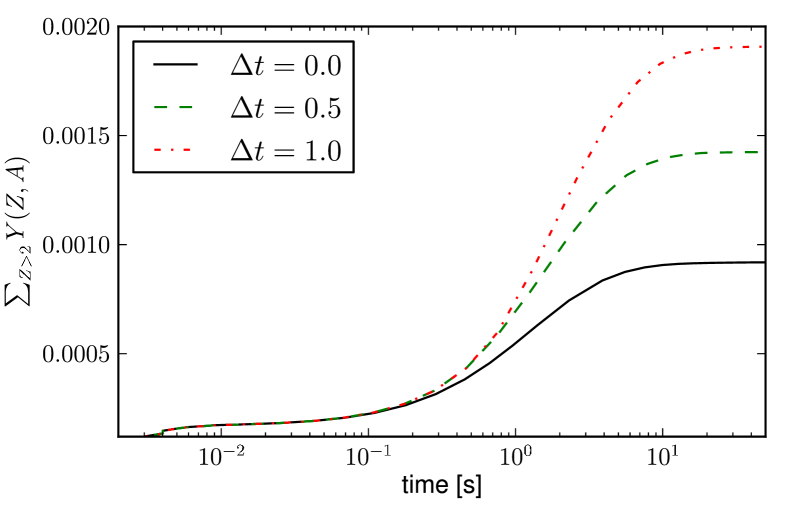
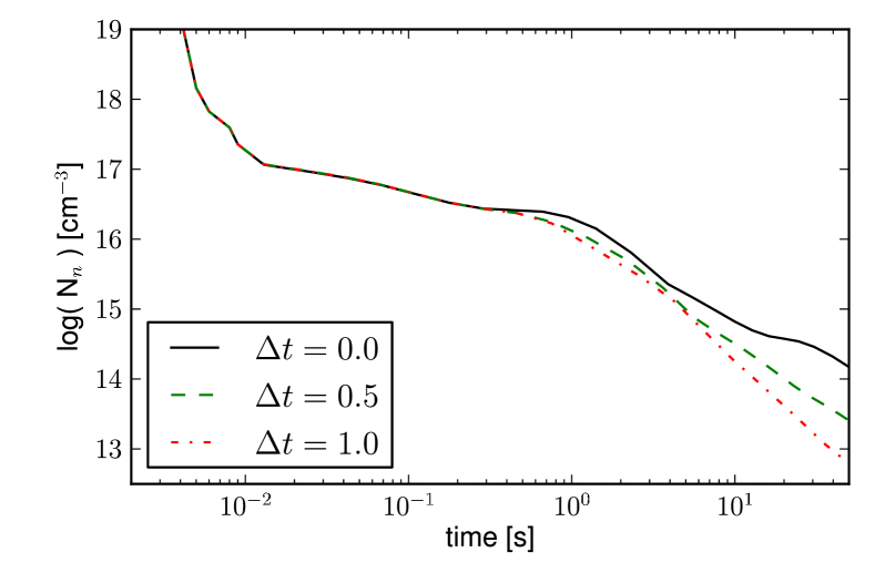
Figure 11: Abundances of $\alpha$ particles (top panel), abundances of heavy nuclei with $Z>2$ (middle panel), and neutron densities (bottom panel) for $\Delta t=0.0$ s (solid black), 0.5 s (dashed green), and 1.0 s (dotted red).

5 Conclusions

We have studied the impact of the supernova dynamical evolution on the $\nu p$-process and how the wind termination affects the synthesis of elements beyond iron. For a robust and strong production of nuclei with $64\lesssim A\lesssim 110$ there is an optimal wind termination temperature at $\approx$2 GK as it was found by Wanajo et al. (2011a). Also in agreement with their work, we have shown that if the wind termination occurs at low temperatures ($T_{\mathrm{wt}}\approx 1$ GK), matter stays too short time in the optimal temperature range for $\nu p$-process nucleosynthesis, $\sim 1-2$ GK. Moreover, the electron antineutrino flux quickly becomes too small to produce the necessary neutrons to overcome the $\beta^{+}$-decay waiting points. This hinders the $\nu p$-process and consequently the efficient synthesis of heavy nuclei. Therefore, the wind termination temperature determines the heaviest elements produced.

We have identified an end point cycle that is key at high temperatures (around 3 GK). The close NiCu cycle inhibits the production of elements heavier than 56Ni. The reactions in this closed NiCu cycle are the following:

$${}^{56}Ni(n,p)^{56}Co(p,\gamma)^{57}Ni(n,p)^{57}Co(p,\gamma)^{58}Ni$$

$$\longrightarrow\,^{58}Ni(p,\gamma)^{59}Cu(p,\alpha)^{56}Ni\,.$$

At high temperatures the reaction ⁵⁹Cu$(p,\alpha)$ ⁵⁶Ni prevents the synthesis of elements beyond the iron group. When the temperature drops below $\approx 3$ GK, ⁵⁹Cu$(p,\gamma)$ ⁶⁰Zn becomes more effective than ⁵⁹Cu$(p,\alpha)$ ⁵⁶Ni. This leads to breakout from the NiCu cycle and the flow of matter can continue towards heavier nuclei. The temperature dependence of these two reactions is critical because it sets the temperature at which the $\nu p$-process can start to synthesize elements beyond Nickel. If this cross-over temperature were slightly higher, matter would be closer to the proto-neutron star and thus under higher neutrino flux when the path starts to move towards heavier nuclei. This will significantly increase the efficiency of the $\nu p$-process. Therefore, our results clearly motivate further investigation of these two key reactions: ⁵⁹Cu$(p,\alpha)$ ⁵⁶Ni and ⁵⁹Cu$(p,\gamma)$⁶⁰Zn. Particularly relevant are the branching ratios for the decay by alpha and gamma emission of compound states in ⁶⁰Zn above the proton separation energy.

We have also explored for the first time the impact of the dynamical evolution after the wind termination on the synthesis of heavy elements by the $\nu p$-process. Hydrodynamical simulations show that after the wind termination there is a transition from an expansion with almost constant temperature and density to a phase with almost constant velocity. The duration of the constant temperature phase, $\Delta t$, strongly affects the final abundances of heavy nuclei. We have found that for $\Delta t=0.0$ s the final flow of matter to stability occurs by neutron capture reactions, i.e $(n,\gamma)$ and $(n,p)$, and not by $\beta^{+}$-decays. When the phase of constant temperature is very short ($\Delta t<0.5$ s), the abundances of nuclei with $64<A<110$ are lower. This leads to significantly higher neutron densities at later times. Depending on the neutron density the matter moves to stability either by $\beta^{+}$-decays ($\Delta t=1.0$ s) or by neutron captures. These two different ways of reaching stability leave a distinct fingerprint in the final abundances.

We have investigated in detail the impact of dynamical evolution on the $\nu p$-process nucleosynthesis using individual characteristic trajectories. In order to predict the complete $\nu p$-process yields from a supernova simulation, one will need to integrate over all proton-rich ejecta.

In summary, the supernova dynamics as well as individual reactions such as the proton capture reactions on ⁵⁹Cu determine how high in proton number the $\nu p$-process can proceed. The dynamical evolution just after the wind termination can greatly affect the nucleosynthesis evolution towards stability as it determines the late neutron density. Our results provide a link between nucleosynthesis in proton-rich winds and the dynamical evolution of the ejected matter and motivate further theoretical and experimental effort on understanding key reactions.

References

- Angulo et al. (1999) Angulo, C., Arnould, M., Rayet, M., Descouvemont, P., Baye, D., Leclercq-Willain, C., Coc, A., Barhoumi, S., Aguer, P., Rolfs, C., et al., 1999, Nucl. Phys. A, 656, 3
- Arcones & Janka (2011) Arcones, A., & Janka, H.-T., 2011, A&A, 526, A160, 1008.0882
- Arcones et al. (2007) Arcones, A., Janka, H.-T., & Scheck, L., 2007, A&A, 467, 1227
- Arcones & Martínez-Pinedo (2011) Arcones, A., & Martínez-Pinedo, G., 2011, Phys. Rev. C, 83, 045809, 1008.3890
- Arcones & Montes (2011) Arcones, A., & Montes, F., 2011, ApJ, 731, 5, 1007.1275
- Duncan et al. (1986) Duncan, R. C., Shapiro, S. L., & Wasserman, I., 1986, ApJ, 309, 141
- Fischer et al. (2010) Fischer, T., Whitehouse, S. C., Mezzacappa, A., Thielemann, F., & Liebendörfer, M., 2010, A&A, 517, A80
- Fröhlich et al. (2006) Fröhlich, C., Martínez-Pinedo, G., Liebendörfer, M., Thielemann, F.-K., Bravo, E., Hix, W. R., Langanke, K., & Zinner, N. T., 2006, Physical Review Letters, 96, 142502
- Fuller et al. (1982) Fuller, G. M., Fowler, W. A., & Newman, M. J., 1982, ApJS, 48, 279
- Hoffman et al. (2008) Hoffman, R. D., Müller, B., & Janka, H.-T., 2008, ApJ, 676, L127, arXiv:0712.4257
- Hoffman et al. (1997) Hoffman, R. D., Woosley, S. E., & Qian, Y.-Z., 1997, ApJ, 482, 951
- Hüdepohl et al. (2010) Hüdepohl, L., Müller, B., Janka, H., Marek, A., & Raffelt, G. G., 2010, Phys. Rev. Lett., 104, 251101
- Langanke & Martínez-Pinedo (2001) Langanke, K., & Martínez-Pinedo, G., 2001, At. Data. Nucl. Data Tables, 79, 1
- Möller et al. (2003) Möller, P., Pfeiffer, B., & Kratz, K.-L., 2003, Phys. Rev. C, 67, 055802
- Otsuki et al. (2000) Otsuki, K., Tagoshi, H., Kajino, T., & Wanajo, S., 2000, ApJ, 533, 424
- Panov & Janka (2009) Panov, I. V., & Janka, H.-T., 2009, A&A, 494, 829, 0805.1848
- Pruet et al. (2006) Pruet, J., Hoffman, R. D., Woosley, S. E., Janka, H.-T., & Buras, R., 2006, ApJ, 644, 1028
- Qian & Wasserburg (2001) Qian, Y.-Z., & Wasserburg, G. J., 2001, ApJ, 559, 925
- Qian & Woosley (1996) Qian, Y.-Z., & Woosley, S. E., 1996, ApJ, 471, 331
- Rauscher & Thielemann (2000) Rauscher, T., & Thielemann, F.-K., 2000, At. Data Nucl. Data Tables, 75, 1
- Roberts et al. (2010) Roberts, L. F., Woosley, S. E., & Hoffman, R. D., 2010, ApJ, 722, 954, 1004.4916
- Schatz et al. (2001) Schatz, H., Aprahamian, A., Barnard, V., Bildsten, L., Cumming, A., Ouellette, M., Rauscher, T., Thielemann, F.-K., & Wiescher, M., 2001, Physical Review Letters, 86, 3471
- Sumiyoshi et al. (2000) Sumiyoshi, K., Suzuki, H., Otsuki, K., Terasawa, M., & Yamada, S., 2000, PASJ, 52, 601
- Thompson et al. (2001) Thompson, T. A., Burrows, A., & Meyer, B. S., 2001, ApJ, 562, 887
- Wanajo (2006) Wanajo, S., 2006, ApJ, 647, 1323
- Wanajo (2007) Wanajo, S., 2007, ApJ, 666, L77, arXiv:0706.4360
- Wanajo et al. (2011a) Wanajo, S., Janka, H.-T., & Kubono, S., 2011a, ApJ, 729, 46, 1004.4487
- Wanajo et al. (2011b) Wanajo, S., Janka, H.-T., & Müller, B., 2011b, ApJ, 726, L15, 1009.1000
- Wanajo et al. (2009) Wanajo, S., Nomoto, K., Janka, H., Kitaura, F. S., & Müller, B., 2009, ApJ, 695, 208, 0810.3999
- Woosley et al. (1994) Woosley, S. E., Wilson, J. R., Mathews, G. J., Hoffman, R. D., & Meyer, B. S., 1994, ApJ, 433, 229