Dynamical r-process studies within the neutrino-driven wind scenario and its sensitivity to the nuclear physics input

Abstract

We use results from long-time core-collapse supernovae simulations to investigate the impact of the late time evolution of the ejecta and of the nuclear physics input on the calculated r-process abundances. Based on the latest hydrodynamical simulations, heavy r-process elements cannot be synthesized in the neutrino-driven winds that follow the supernova explosion. However, by artificially increasing the wind entropy, elements up to $A=195$ can be made. In this way one can reproduce the typical behavior of high-entropy ejecta where the r-process is expected to occur. We identify which nuclear physics input is more important depending on the dynamical evolution of the ejecta. When the evolution proceeds at high temperatures (hot r-process), an $(n,\gamma)\rightleftarrows(\gamma,n)$ equilibrium is reached. While at low temperature (cold r-process) there is a competition between neutron captures and beta decays. In the first phase of the r-process, while enough neutrons are available, the most relevant nuclear physics input are the nuclear masses for the hot r-process and the neutron capture and beta-decay rates for the cold r-process. At the end of this phase, the abundances follow a steady beta flow for the hot r-process and a steady flow of neutron captures and beta decays for the cold r-process. After neutrons are almost exhausted, matter decays to stability and our results show that in both cases neutron captures are key for determining the final abundances, the position of the r-process peaks, and the formation of the rare-earth peak. In all the cases studied, we find that the freeze out occurs in a timescale of several seconds.

I Introduction

The synthesis of heavy elements by the rapid neutron capture process (r-process) is a fascinating, long-standing problem which involves challenges in nuclear physics (experiment and theory), astrophysical simulations of explosive environments, and observations of metal-poor stellar atmospheres. The astrophysical site where the r-process produces half of the heavy elements has not yet been identified (see Ref. Arnould et al. (2007) for a recent review). However, even if the astrophysical scenario were discovered, one still has to deal with nuclei far from stability for which no experimental data are available and theoretical predictions are quite uncertain Grawe et al. (2007).

Galactic chemical evolution models Wanajo and Ishimaru (2006); Qian and Wasserburg (2007) indicate that heavy elements are most likely produced in core-collapse supernova outflows. After a core-collapse supernova explosion, a proto-neutron star forms and a baryonic neutrino-driven wind develops Duncan et al. (1986). The matter expands at high velocity, which can become supersonic, and eventually collides with the slow, early supernova ejecta resulting in a wind termination shock or reverse shock Burrows et al. (1995); Janka and Müller (1996); Buras et al. (2006); Arcones et al. (2007); Fischer, T. et al. (2010). There are several nucleosynthesis process that occur or might occur in this environment: $\alpha$-process Woosley and Hoffman (1992); Witti et al. (1994), $\nu$p-process Fröhlich et al. (2006a); Pruet et al. (2006); Wanajo (2006), and r-process Woosley et al. (1994); Takahashi et al. (1994). The production of heavy r-process elements ($A>130$), requires a high neutron-to-seed ratio. This can be achieved by the following conditions Qian and Woosley (1996); Hoffman et al. (1997); Otsuki et al. (2000); Thompson et al. (2001): high entropy, fast expansions, or low electron fraction. However, these conditions are not yet realized in hydrodynamical simulations that follow the outflow evolution during the first seconds of the wind phase after the explosion Arcones et al. (2007); Hüdepohl et al. (2010); Fischer, T. et al. (2010).

This manuscript aims to explore the sensitivity of the calculated r-process abundances to the combined effects of the long-time dynamical evolution and nuclear physics input providing a link between the behavior of nuclear masses far from stability and features in the final abundances. The impact of the nuclear physics input on the production of heavy elements has been explored in classical r-process calculations in Ref. Kratz et al. (1993, 1998) and with more dynamical but still parametric calculations (e.g., Howard et al. (1993); Freiburghaus et al. (1999); Meyer and Brown (1997)). However, most of the r-process studies Arnould et al. (2007) aimed to find the astrophysical conditions (density, temperature, electron fraction) that reproduce the solar abundances for a given nuclear physics input. There have been only few works exploring the impact of different mass models (e.g., Wanajo et al. (2004); Farouqi et al. (2010)), the effect of neutron captures when matter decays to stability Surman et al. (1997); Surman and Engel (2001); Surman et al. (2009); Beun et al. (2009a), and the importance of beta decays Borzov et al. (2008); Dillmann et al. (2003). Our results contribute to improve the present understanding of how nuclear masses and neutron-capture cross sections determine the r-process abundances. The influence of the beta-decay rates will be studied in future work, here we only explore the effect of beta-delayed neutron emission.

In this paper we use hydrodynamical trajectories from the neutrino-driven wind simulations of Ref. Arcones et al. (2007). As the conditions found in these trajectories do not allow for the synthesis of heavy r-process elements Arcones and Montes (2010), we artificially increase the entropy by a factor two in order to produce the third r-process peak. This allows us to study the nucleosynthesis of heavy elements in a typical high-entropy neutrino-driven wind in a more consistent way than with fully parametric expansions Freiburghaus et al. (1999); Farouqi et al. (2010) or with steady-state wind models (e.g. Otsuki et al. (2000); Thompson et al. (2001)), which cannot consistently explore the interaction of the wind with the slow supernova ejecta. The possible influence of the wind termination shock on the nucleosynthesis was already suggested in Refs. Janka and Müller (1996); Qian and Woosley (1996) and analyzed in different works Terasawa et al. (2002); Wanajo et al. (2002); Wanajo (2007); Kuroda et al. (2008); Panov and Janka (2009). For the first time, we use here trajectories obtained in hydrodynamical simulations to perform a detailed investigation of the effect on the r-process of the long-time dynamical evolution. We choose two different astrophysical evolutions, that cover the broad range of conditions found in the hydrodynamical simulations. Four different mass models are used to study the impact of the nuclear physics input on the calculated abundances.

Our astrophysical and nuclear physics inputs are introduced in Sect. II. We study the impact on the final abundances of the reverse shock and long-time dynamical evolution (Sect. III.1). The sensitivity of the abundances and of the r-process evolution to the mass model is explored in Sect. III.2. In Sect. III.3, we discuss the evolution of the abundances after the r-process freeze-out, that we define as the moment when the neutron-to-seed ratio drops below one. Our conclusions are summarized in Sect. IV.

II Methods

II.1 Neutrino-driven wind and termination shock

Our nucleosynthesis studies are based on a trajectory ejected at 8 s after bounce in an explosion of a 15 $M_{\odot}$ progenitor (model M15-l2-r1 in Arcones et al. (2007)). This trajectory represents a typical neutrino-driven wind, whose wind phase can be described by steady-state models Qian and Woosley (1996); Otsuki et al. (2000); Thompson et al. (2001); Wanajo et al. (2001). However, hydrodynamical simulations are required to study the long-time evolution when the supersonic wind collides with the slow-moving supernova ejecta resulting in a wind termination shock.

Detailed description of the hydrodynamical simulations can be found in Refs. Arcones et al. (2007); Scheck et al. (2006). In these simulations, Newtonian hydrodynamics Scheck et al. (2006); Kifonidis et al. (2006) with general relativistic corrections for the gravitational potential Marek et al. (2006) is combined with a simplified neutrino transport approximation assuming Fermi-Dirac neutrino spectra Scheck et al. (2006). This is computationally very efficient and reproduces the results of Boltzmann transport simulations qualitatively. The equation of state used in the simulations includes neutrons, protons, alpha particles, and a representative nucleus (${}^{54}\text{Mn}$) treated as non-relativistic Boltzmann gases in nuclear statistical equilibrium Janka and Müller (1996). The central part ($\rho\gtrsim 10^{13}\,\text{g}/\text{cm}^{3}$) of the proto-neutron star is removed from the computational domain and a Lagrangian inner boundary (placed below the neutrinosphere) describes the neutron star evolution. The neutrino cooling (i.e., neutrino energies and luminosities) and contraction of the proto-neutron star are parametrized at the inner boundary to account for possible uncertainties in the high density equation of state.

The neutron-to-seed ratio found in the simulations of Ref. Arcones et al. (2007) after freeze-out of charged-particle reactions is too low ($Y_{n}/Y_{\rm{seed}}\approx 10^{-2}$) to permit the formation of heavy r-process nuclei. Only elements with $Z<48$ are produced, i.e. light element primary process (LEPP) elements Arcones and Montes (2010). However, we can still use this trajectory for r-process studies, if the neutron-to-seed ratio is artificially increased by assuming a smaller initial electron fraction or by rising the entropy. The electron fraction is determined by electron neutrino and antineutrino energies and luminosities (see e.g., Ref. Qian and Woosley (1996)) and we keep it as given by the simulations ($Y_{e}\approx 0.47$). Hereafter, all calculations are performed on the same trajectory with the density decreased by a factor of two  overall to get also a factor two higher entropies ($S\propto T^{3}/\rho\approx 200\ k_{B}/\mathrm{nuc}$) and thus high neutron-to-seed ratio ($Y_{n}/Y_{\mathrm{seed}}\approx 70$). This is enough to produce nuclei around the $A=195$ peak and mimics the hydrodynamical conditions of a neutrino-driven wind where the r-process does occur and of other astrophysical environments that involve ejection of high entropy matter. Therefore, it can be used as basis to study the combined influence on the abundances of the long-time dynamical evolution and of the nuclear physics input.

Variations in the late evolution of the ejecta are expected as shown in multidimensional simulations Arcones and Janka (2010). Although the neutrino-driven wind stays spherically symmetric in absence of rotation, the interaction of the wind with the slow, early supernova ejecta and thus the resulting reverse shock depends on the progenitor structure Arcones et al. (2007) and on the anisotropic pressure distribution of the supernova ejecta, where the wind propagates through Arcones and Janka (2010). Since our trajectory corresponds to a spherically symmetric simulation, we have modified it to account for the possible variation of the reverse shock radius and of the long-time evolution. The changes are done only after charged-particle reactions freeze out to assure same initial conditions for the r-process.

As we will show, the reverse shock has a non-negligible influence on nucleosynthesis. When the wind collides with the slow-moving ejecta, the expansion velocity drops as kinetic energy is transformed into internal energy, with the consequent increase in temperature and density. The density ($\rho_{\text{rs}}$), temperature ($T_{\text{rs}}$), and velocity ($u_{\text{rs}}$) of the shocked matter can be calculated with the Rankine-Hugoniot conditions, corresponding to mass, momentum, and energy conservation:

$$\rho_{\text{w}}u_{\text{w}} =\rho_{\text{rs}}u_{\text{rs}}\,,$$ (1a)

$$P_{\text{w}}+\rho_{\text{w}}u_{\text{w}}^{2} =P_{\text{rs}}+\rho_{\text{rs}}u_{\text{rs}}^{2}\,,$$ (1b)

$$\frac{1}{2}u_{\text{w}}^{2}+\epsilon_{\text{w}}+\frac{P_{\text{w}}}{\rho_{\text{w}}} =\frac{1}{2}u_{\text{rs}}^{2}+\epsilon_{\text{rs}}+\frac{P_{\text{rs}}}{\rho_{\text{rs}}}\,,$$ (1c)

here $\rho$, $u$, $P$, and $\epsilon$ are the density, velocity, pressure, and specific internal energy, respectively. Quantities in the wind have the subscript “w” and in the shocked material, above the reverse shock, the subscript “rs”. In addition to these equations, one needs an equation of state that relates pressure and energy. In the last equation we take $\epsilon\approx 3P/\rho$ which is a good approximations because the environment is radiation-dominated. The lhs of these equations is known from the wind, therefore we combine them to obtain two possible solutions for the matter velocity after the shock: 1) $u_{\text{rs}}=u_{\text{w}}$, no shock; 2) $u_{\text{rs}}=u_{\text{w}}/7+8/7\,P_{\text{w}}/(\rho_{\text{w}}u_{\text{w}})$. Once the velocity is known, the density and pressure of the shocked matter are calculated with Eqs. (1a), (1b). Any other thermodynamical variable, including temperature and entropy, can be obtained from an equation of state (EoS). Here, we use the Timmes EoS Timmes and Arnett (1999).

Once the conditions of the shocked matter are known, we need to describe their evolution. The density and velocity evolutions have to fulfill the condition of constant mass outflow ($\dot{M}=4\pi r^{2}v\rho$). Two extreme expansions can be identified: 1) the velocity is constant, and the density thus decreases as $r^{-2}$; 2) the density is constant and then it is the velocity that decreases as $r^{-2}$. The latter expansion was used in Ref. Kuroda et al. (2008) but it implies a decrease of the velocity down to a few m s^-1 in about a second, while in full hydrodynamical simulations Arcones et al. (2007); Fischer, T. et al. (2010), the velocities stay around $10^{3}$–$10^{4}$ km s^-1. Following these simulations, we prescribe an extrapolation for the evolution of matter which is between these two extreme cases. The density of the shocked matter stays constant and the velocity decreases as $r^{-2}$ during one second. Afterwards, we keep the velocity constant and the density decreases as $r^{-2}$. A similar extrapolation is obtained with the prescription used in Ref. Wanajo et al. (2010).

II.2 Nucleosynthesis network and nuclear physics input

We start our nucleosynthesis calculations at a temperature $T=10$ GK where the composition is given by nuclear statistical equilibrium and is dominated by free neutrons and protons. The evolution of the composition is followed with two reactions networks. During the seed formation we use an extended network that includes all possible charged-particle reactions. While for the r-process we take advantage of a faster network that only considers neutron capture, beta decay, photodissociation, alpha decay, and fission. However, fission reactions play a negligible role in the present calculations and will not be further discussed.

The extended nuclear reaction network consists of 3347 nuclei from neutron and protons to Europium. Neutral and charged-particle reactions are the same as in the REACLIB compilation used by (Fröhlich et al., 2006b). For the weak-interaction rates (electron/positron captures and $\beta$-decays) we use the rates of Refs. Fuller et al. (1982a, b) for nuclei with $A\leq 45$ and those of Refs. Langanke and Martínez-Pinedo (2000, 2001) for $45<A\leq 65$. Neutrino interactions are important during the seed formation since they control the amount of free neutrons and are taken from Ref. Zinner (2007). When the temperature drops below $T\sim 3$ GK charged-particle reactions freeze out, i.e end of the $\alpha$-process Woosley and Hoffman (1992); Witti et al. (1994), and the r-process phase, characterized by a domination of neutron capture, begins. The subsequent evolution is followed by a r-process network of 5300 nuclei between $Z=14$ and $Z=110$. Since we are interested in the detailed evolution of matter when decays to stability, we had to improve the original network of D. Mocelj PhD Mocelj (2007). This network was based on the algorithm suggested by Ref. Cowan et al. (1983) which is also used in Refs. Freiburghaus et al. (1999); Farouqi et al. (2010). Such algorithm assumes that the neutron abundance ($Y_{n}$) stays constant during a time step (see Appendix). This is very efficient during the early r-process phase, but it becomes numerically unstable when the neutron-to-seed ratio drops below one and $Y_{n}$ decreases very fast. This problem can be cured using smaller time steps, which increases however the computational time without completely removing the numerical instabilities. In our updated network, the equation for the neutron abundance evolution (see Eq. 9) is included and the resulting system of equations is solved using a fully implicit scheme based on the Newton-Raphson method Hix and Thielemann (1999); Hix and Meyer (2006) and the sparse matrix solver package PARDISO Schenk and Gärtner (2004).

Our nucleosynthesis calculations are based on four different mass models and their consistently calculated neutron capture rates: the Finite Range Droplet Model (FRDM) (Möller et al., 1995), the quenched version of the Extended Thomas-Fermi with Strutinsky Integral (ETFSI-Q) (Pearson et al., 1996), the version 17 of the Hartree-Fock-Bogoliubov masses (HFB-17) (Goriely et al., 2009), and the Duflo-Zuker mass formula (Duflo and Zuker, 1995). For the FRDM and ETFSI-Q mass models the neutron-capture rates are taken from Ref. Rauscher and Thielemann (2000) that uses the statistical model code NON-SMOKER Rauscher and Thielemann (1998). The HFB-17 neutron capture rates are taken from the Bruslib database  and were computed with the statistical model code TALYS (Goriely et al., 2008). For the Duflo-Zuker mass formula, we have evaluated the neutron-capture rates using the analytic approximation suggested in Ref. Michaud and Fowler (1970) that reproduces the results of more sophisticated statistical model calculations (Woosley et al., 1975; Mathews et al., 1983) (see also Sect. III.3). For the range of temperatures we are considering, the temperature dependence of the $(n,\gamma)$ rates can be neglected and we use thus values that correspond to a temperature of 30 keV. The inverse $(\gamma,n)$ rates are obtained from detailed balance (see Eq. 8).

We use theoretical beta-decay rates from Ref. Möller et al. (2003) supplemented by experimental data whenever available (NuDat 2 database (NuDat2, 2009)). We realize that the beta decays should be calculated consistently with the mass model, however such calculations have not been performed so far. We plan to explore the sensitivity of r-process calculations to different beta-decay rates in future work.

III Results

III.1 Wind termination shock and long-time evolution

Here we analyze the impact of the reverse shock on the r-process abundances and dynamics. All calculations presented in this section are based on the ETFSI-Q mass model.

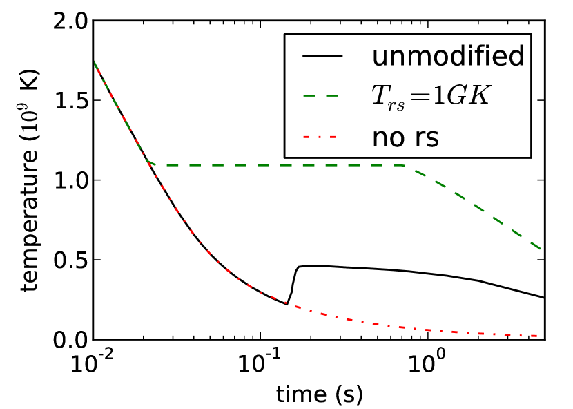
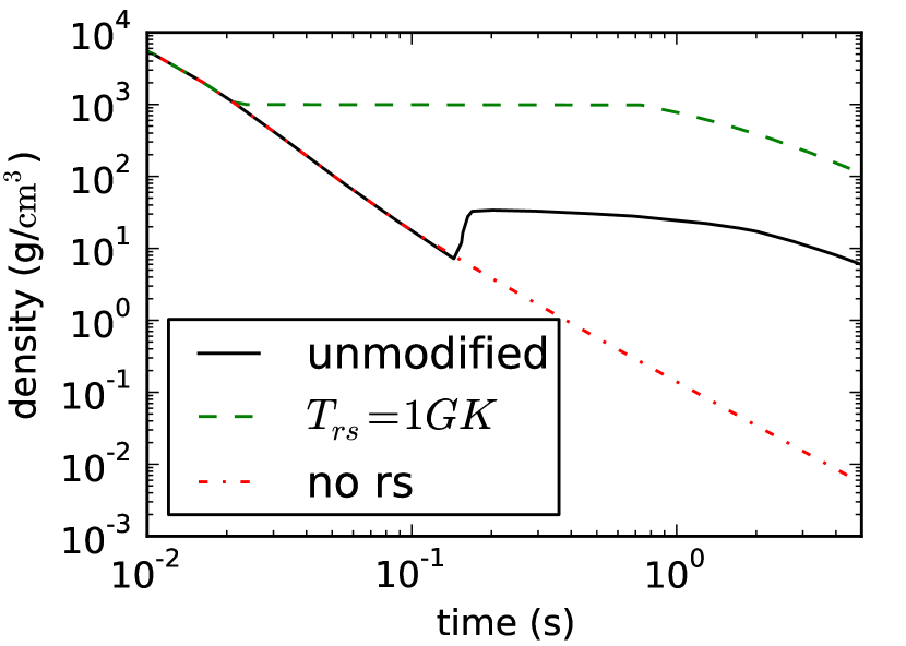
Figure 1: (Color online) Temperature and density evolution of a mass element ejected at 8 s after bounce of the supernova explosion based on model M15-l2-r1 of Ref. Arcones et al. (2007), see discussion in Sect. II. The solid black line corresponds to the original trajectory from the supernova simulation labeled as “unmodified”. Notice, that density have been divided by a factor 2 to get higher neutron-to-seed ratio. The green dashed line represents a evolution with the reverse shock at temperature of 1 GK. For the evolution shown by the red dashed-dotted line the reverse shock was removed.

Our nucleosynthesis study correspond to the trajectories shown in Fig. 1. The solid black line, labeled as “unmodified”, represents the trajectory from Ref. Arcones et al. (2007) introduced in Sect. II.1. The position of the reverse shock and the evolution after it are not modified, but the density is overall reduced by a factor of two. In the dashed green line the reverse shock is assumed to be at temperature of 1 GK and the subsequent evolution is calculated as described in Sect. II.1. The dashed-dotted red line, labeled as “no rs”, reproduces a case without reverse shock, where matter expands without colliding with the slow, early supernova ejecta. In this case, we assume an adiabatic (constant entropy) expansion with constant velocity starting at the position of the reverse shock in the simulation. As the mass outflow is constant, the density decreases with radius as $\rho\propto r^{-2}$.

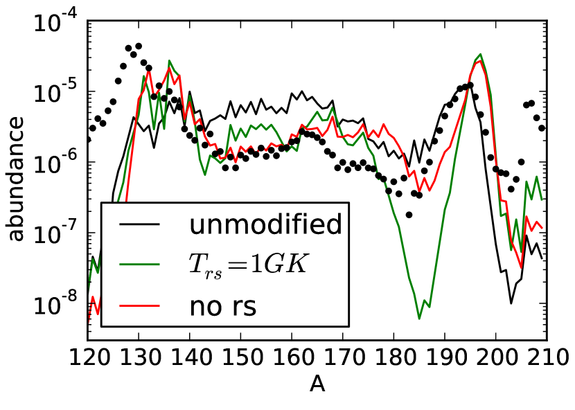
Figure 2: (Color online) Final abundances for the different evolutions of Fig. 1 compared to solar r-process abundances shown by dots.

Figure 2 shows the final r-process abundances for the different trajectories together with solar r-process abundances (dots) Sneden et al. (2008). None of the calculations reproduce the solar abundances around the second peak ($A\sim 130$), since we have chosen the conditions which produce mainly the third r-process peak ($A\sim 195$). A pattern similar to solar is expected from a superposition of different trajectories Freiburghaus et al. (1999); Wanajo et al. (2001). Some of the deficiencies seen in Fig. 2 are due to the mass model and will be discussed in the next section. However, there are features that depend on the dynamical evolution. In order to understand the abundances under different late time evolutions (Fig. 1), we look at the characteristic timescales for the r-process: neutron capture, photodissociation, and beta decay that are defined, respectively, as:

$$\frac{1}{\tau_{(n,\gamma)}} = \frac{\sum_{Z,A}N_{n}\langle\sigma v\rangle_{(Z,A)}Y(Z,A)}{\sum_{Z,A}Y(Z,A)},$$ (2a)

$$\frac{1}{\tau_{(\gamma,n)}} = \frac{\sum_{Z,A}\lambda_{\gamma}(Z,A)Y(Z,A)}{\sum_{Z,A}Y(Z,A)},$$ (2b)

$$\frac{1}{\tau_{\beta}} = \frac{\sum_{Z,A}\lambda_{\beta}(Z,A)Y(Z,A)}{\sum_{Z,A}Y(Z,A)},$$ (2c)

where $N_{n}$ is the neutron number density, $\langle\sigma v\rangle_{(Z,A)}$ the neutron capture or $(n,\gamma)$ rate, $\lambda_{\gamma}(Z,A)$ the photodissociations or $(\gamma,n)$ rate, and $\lambda_{\beta}(Z,A)$ the beta-decay rate. The evolution of these timescales is shown in Fig. 3 for the trajectories labeled as “$T_{rs}=1$ GK” (left panel) and “unmodified” (right panel). The trajectory labeled “no rs” follows a behavior very similar to the unmodified one.

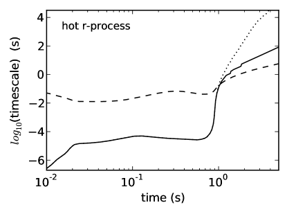
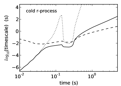
Figure 3: Evolution of relevant timescales for the trajectories shown in Fig. 1 and labeled as “$T_{\mathrm{rs}}=1$ GK” (left panel) and “unmodified” (right panel). Solid, dashed, and dotted lines represent the neutron capture, beta decay, and photodissociation timescales, respectively.

For the trajectory with the reverse shock at $T=1$ GK (Fig. 3, left panel), there is a competition between neutron captures and photodissociation that last until neutrons are exhausted at around 1 s. During this evolution under $(n,\gamma)\rightleftarrows(\gamma,n)$ equilibrium, the beta-decay timescale is longer than the other two, i.e. $\tau_{(n,\gamma)}=\tau_{(\gamma,n)}\ll\tau_{\beta}$. In the following, this kind of evolution is called hot r-process. When the reverse shock is at lower temperatures (Fig. 3, right panel), the photodissociation timescale becomes longer than the other two timescales once the temperature drops below $\sim 0.5$ GK. The subsequent evolution proceeds by a competition between beta decay and neutron capture, i.e. $\tau_{(n,\gamma)}\approx\tau_{\beta}\ll\tau_{(\gamma,n)}$. This evolution was already studied in Ref. Blake and Schramm (1976) and has been recently named as cold r-process Wanajo (2007) and rn-process Panov and Janka (2009). We call this evolution cold r-process.

The relevant nuclear physics input depends on the dynamical evolution. The hot r-process proceeds initially in $(n,\gamma)\rightleftarrows(\gamma,n)$ equilibrium, therefore the neutron separation energy is the key quantity that determines the location of the r-process path, see Eq. (10). For the cold r-process the evolution proceeds by a competition between neutron captures and beta decays. Therefore, the most relevant nuclear physics inputs are beta-decay and neutron-capture rates. Nuclear masses are also important because they enter in the calculation of both. The evolution after freeze out is dominated by beta decays and neutron captures for both cold and hot r-process.

The final abundances shown in Fig. 2 indicate that cold r-process calculations lead to broader peaks because the r-process proceeds farther away from stability. The hot r-process, which evolves in $(n,\gamma)\rightleftarrows(\gamma,n)$ equilibrium, results in a huge trough in the abundances before the third r-process peak (green line in Fig. 2). This is due to the behavior of the neutron separation energy just before the $N=126$ shell closure (see Fig. 6) and will be discussed in the next section.

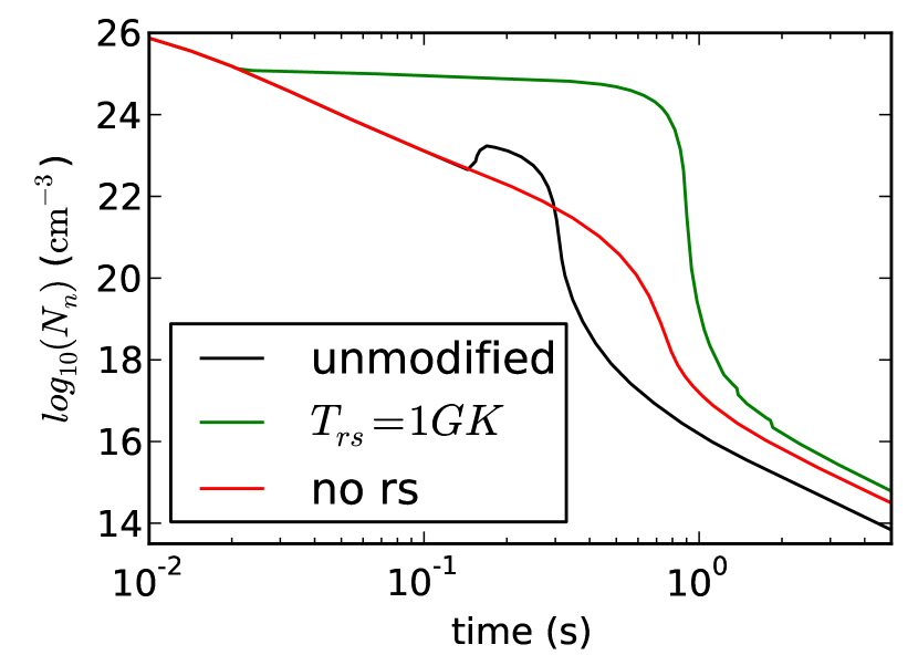
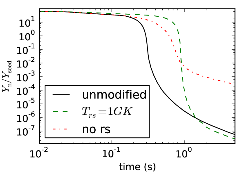
Figure 4: (Color online) Neutron density, neutron-to-seed ratio, and average neutron separation energy evolution (Eq. (3)) for the same trajectories shown in Fig. 1.

After we have introduced the two possibilities for the r-process: hot and cold, the evolution of relevant quantities (neutron density, neutron-to-seed ratio, and average neutron separation energy) will be explained. The average neutron separation energy (shown in the bottom panel of Fig. 4) is defined as:

$$\langle S_{n}\rangle=\frac{\sum_{Z,A}S_{n}(Z,A)Y(Z,A)}{\sum_{Z,A}Y(Z,A)},$$ (3)

where $S_{n}(Z,A)$ is the neutron separation energy of a nucleus with mass number $A$ and charge number $Z$, and $Y(Z,A)$ is its abundance. The neutron separation energy is smaller for nuclei far from stability, since their neutrons become less bound. Therefore, we can use this quantity to study the evolution of the r-process.

We consider first the hot r-process which is labeled as “$T_{\mathrm{rs}}=1$ GK” in Figs. 1, 2, and 4. The average neutron separation energy (Fig. 4, bottom panel) decreases very fast initially, as matter moves away from stability after charged-particle reactions freeze out. $\langle S_{n}\rangle$ comes to a minimum after 30 ms, because the matter flow has reached $N=82$ shell closure. Here the abrupt drop of individual neutron separation energies and the high photodissociation rates prevent matter to move farther away from stability. Therefore, the r-process path moves to higher Z by beta decays and successive neutron captures, while the neutron number stays constant at $N=82$. This is shown in Fig. 6 by the dots that mark the r-process path. Once the neutron separation energy for nuclei beyond $N=82$ becomes large enough, the flow of matter can continue moving towards heavier nuclei. The r-process path reaches the $N=126$ shell closure at around 500 ms as indicated by the second minimum in $\langle S_{n}\rangle$. When matter starts to pass through the $N=126$ shell closure, neutrons are exhausted in our calculations and the matter decays to stability.

The evolution of the average neutron separation energy for the other two trajectories (cold r-process) is very different because photodissociation becomes negligible once the temperature is $\lesssim 0.5$ GK. The evolution proceeds by a competition of neutron captures and beta decays and this allows matter to move farther from stability compared to the hot r-process. Therefore, the average beta-decay lifetime becomes shorter which speeds up the flow of matter towards heavier nuclei and broadens the minimum in $\langle S_{n}\rangle$. The faster evolution leads to a more rapid decrease of the neutron-to-seed ratio (Fig. 4, middle panel) and therefore the r-process ends earlier than in the hot r-process.

The case without reverse shock (red line in Fig. 1) is extreme because the neutron density decreases initially very fast (Fig. 4, upper panel). This leads to a drop of the neutron captures, which explains the high values of the neutron density and neutron-to-seed ratio that are maintained at later times. Having a large neutron-to-seed ratio at late times allows a continuation of neutron captures, even after several seconds. Therefore, the peak at $A=195$ is shifted towards higher mass numbers as shown in Fig. 2 (see also discussion in Ref. Surman and Engel (2001)). In the hot r-process, neutron captures after freeze-out also lead to the shift of the third peak, even when the r-process path at freeze-out is located at a neutron separation energy of $S_{n}=2.8$ MeV, similar to the one used in the classical r-process calculations of Ref. Kratz et al. (1993), where the peak in the final abundances is obtained at the right position.

III.2 Influence of the mass model

Nuclear masses are a key nuclear physics input for r-process calculations as they determine the energy thresholds for all relevant reactions: neutron capture, photodissociation, and beta decay. In this section we present results based on the four mass models introduced in Sect. II.2 and link features in the abundances with the behaviour of the two neutron separation energy ($S_{2n}$). In the r-process evolution, two phases can be distinguished depending on whether the neutron-to-seed ratio is larger or smaller than one, i.e. before and after freeze-out. The abundances at freeze-out (shown in Fig. 5 by black lines) contain the information of the pre-freeze-out phase when there are enough neutrons to be captured by each individual nucleus. After freeze-out, there are two important facts to be considered: 1) nuclei compete for capturing the few neutrons available, 2) the neutron-capture and beta-decay rates are comparable. These two facts are common to the hot and cold r-process and are important for determining the final abundances shown in Fig. 5 by the green lines. Here we focus on the difference among mass models and general features will be described in the next section.

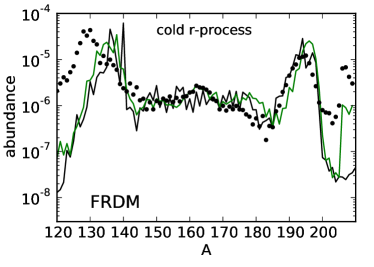
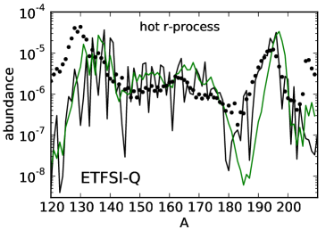
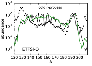
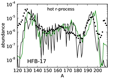
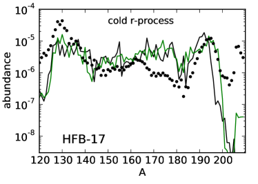
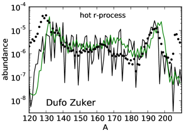
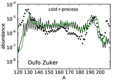
Figure 5: (Color online) Freeze-out (black lines) and final (green lines) abundances for the hot (left column) and cold (right column) r-process. The calculations are based on the mass model that is indicated in the label.

Figure 5 shows the abundances obtained using the four mass models for the hot (left column) and cold (right column) r-process. The freeze-out abundances (black lines) are characterized, especially in the hot r-process, by the presence of strong fluctuations that have almost disappeared in the final abundances (green lines), as expected from solar r-process abundances. These fluctuations are due to the fact that $(n,\gamma)$ and $(\gamma,n)$ reactions favor nuclei with an even neutron number. Consequently, as Z increases in moving from one isotopic chain to the next, N increases by at least two units (except at the magic numbers where it stays constant). Therefore, some mass numbers are not present in the r-process path as shown by the dots in Fig. 6.

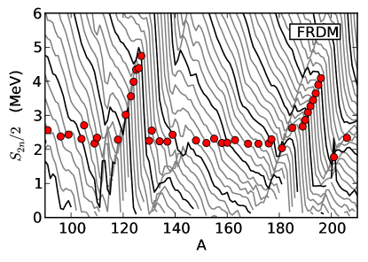
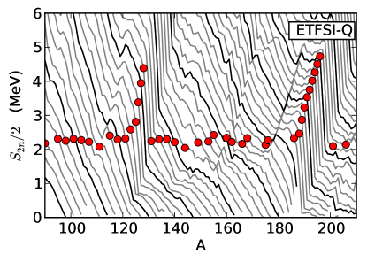
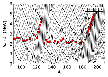
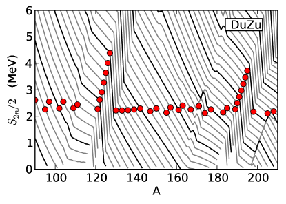
Figure 6: (Color online) Two neutron separation energy for constant proton number as a function of mass number. Black lines correspond to proton numbers starting at Z = 30 on the left and increasing in steps of 5 and grey lines are shown in steps of 1. The hot r-process path is shown at freeze-out ($Y_{n}/Y_{\mathrm{seed}}=1$) by dots.

The freeze-out abundances can be understood looking at the two neutron separation energy in Fig. 6. Two kind of features in $S_{2n}$ leave a fingerprint on the abundances: 1) The abrupt drop in $S_{2n}$ at the magic numbers $N=82$ and $N=126$, leads to accumulation of matter at these neutron numbers and to the formation of peaks in the abundance distribution. 2) In regions where $S_{2n}$ is constant or presents a saddle point behaviour, an equilibrium can not be achieved between neutron captures and photodissociation. In the hot r-process, this leads to troughs in the abundances around $A\sim 110,140$ for the FRDM mass model and around $A\sim 185$ for FRDM, ETFSI-Q, and HFB-17 mass models. These features of the two-neutron separation energies have less impact for the cold r-process because photodissociation reactions are suppressed due to the low temperatures.

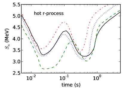
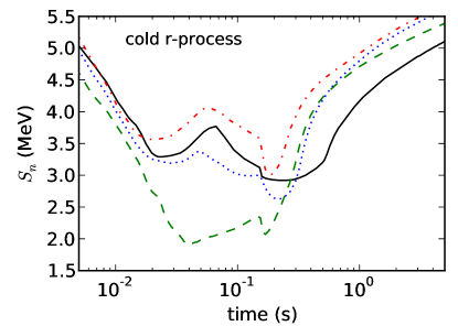
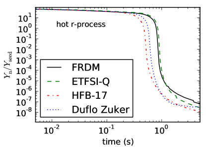
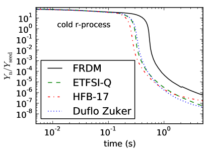
Figure 7: (Color online) Evolution of the average neutron separation energy and neutron-to-seed ratio for the hot (left column) and cold (right column) r-process and based on the four mass models discussed in the text.

We use the average neutron separation energy and the neutron-to-seed ratio (see Fig. 7) to discuss the evolution of matter during the r-process for different mass models in the hot r-process. The average neutron separation energy, $\langle S_{n}\rangle$, shows two minima and one maximum for all mass models. However, $\langle S_{n}\rangle$ significantly differs during the early evolution in the calculation based on ETFSI-Q nuclear masses. For $t\approx 30$ ms, when matter flow approaches $N=82$ shell closure, $\langle S_{n}\rangle$ is smaller and the minimum is broader. Due to the quenching of the $N=82$ shell gap introduced in the ETFSI-Q mass model Pearson et al. (1996), the abrupt drop in $S_{2n}$ at $N=82$ dissapears for $Z<43$ (see Fig. 6). Consequently, with this mass model the r-process proceeds through nuclei with smaller neutron separation energy before reaching the $N=82$ shell closure. This occurs at $Z=43$ for ETFSI-Q, while for the other mass models it is reached already for $Z=40$. The width of the first minimum is related to the sum of half-lives of the nuclei on the r-process path with $N<82$. This is substantially larger in the calculations with ETFSI-Q mass model. There is thus a delay in the time required to overcome the $N=82$ shell closure and a slow down of the speed at which neutrons are captured. Therefore, the r-process freeze-out occurs at later times for ETFSI-Q than for HFB-17 and Duflo-Zuker. The situation is different for FRDM. Here the neutron separation energy drops abruptly just before $N=90$ and even becomes negative for nuclei like ¹³³Pd, ¹³⁴Ag, and ¹³⁷Cd. This region is reached when the r-process breaks out of the $N=82$ shell closure. As the beta-decay half-lives of these nuclei are relatively long (around 100 ms for the rates used in the present calculation Möller et al. (2003)) matter accumulates producing peaks at ¹³⁸Sn in the hot r-process calculation and at ¹³⁴Cd and ¹⁴⁰Sn in the cold r-process (see upper panels of Fig. 5). These nuclei represent a barrier to the flow of neutron captures to more neutron-rich isotopes and consequently the matter has to wait for their beta-decay before heavier nuclei can be reached. This effect results in a broader second minima for the FRDM average neutron separation energy in Fig. 7 and in a longer duration for the r-process.

In the phase after freeze-out, the few available neutrons are not equally captured in all regions. This leads to different position of troughs and peaks depending on the mass model used. The most visible feature in the final abundances is the trough in the ETFSI-Q abundances before the third peak. This is also present in the freeze-out abundances based on FRDM and HFB-17, but not on Duflo-Zuker. During the decay to stability the trough is filled when using the FRDM and HFB-17 mass models while for the ETFSI-Q becomes even larger. The two neutron separation energies in Fig. 6 show that for FRDM there is a drop of $S_{2n}$ for $N=122$ followed by a rise before the $N=126$ magic shell. This leads to the formation of the trough at $A\sim 184$. For ETFSI-Q the two neutron separation energies are almost constant for nuclei in the region $A=180$–190 and $Z\sim 60$. This produces two troughs in the freeze-out abundances at $A=180$ and $A=187$. The situation is more complicated for HFB-17 (as the neutron separation energies show larger fluctuations) with the net result of troughs at $A=180$ and $A=184$ in the freeze-out abundances.  During the decay to stability, in the calculations based on FRDM, HFB-17, and Duflo-Zuker neutron captures move matter from the region before the trough to higher mass numbers and the trough is partially filled. In contrast, ETFSI-Q presents higher $S_{2n}$ (and thus higher $(n,\gamma)$ rates) in the region just before $N=126$. This leads to a shift of matter from the trough towards the peak that produces an enhancement of the first one.

Notice that Duflo-Zuker abundances present stronger odd-even effects than the abundances calculated with the other models as shown in bottom panels of Fig. 5. However, this effect is not due to the mass model itself but to the computed neutron-capture rates, which here are based on the simple approximation suggested in Ref. Michaud and Fowler (1970). The importance of neutron-capture rates on the final abundance will be discussed in detail in Sects. III.3 and III.3.1.

III.3 Decay to stability

As we have shown in the previous section, there are still reactions occurring after freeze out that contribute to the redistribution of matter and to the production of the final abundances. Classical r-process studies (see for example Ref. Kratz et al. (1993), but still amply used for r-process chronometers studies Schatz et al. (2002); Roederer et al. (2009)) neglect the neutron captures after freeze out and consider that beta-delayed neutron emission is the only mechanism to redistribute and smooth the abundances after freeze-out. Dynamical r-process calculations Freiburghaus et al. (1999) have shown that neutron captures during freeze-out can reduce odd-even effects but also shift the peaks Surman and Engel (2001) and produce the small rare-earth peak around $A\approx 160$ Surman et al. (1997). However, in some of these studies (e.g., Freiburghaus et al. (1999); Farouqi et al. (2010)) neutron captures were suppressed once the $Y_{n}/Y_{\text{seed}}$ ratio was small and only beta-decays were considered. Here, we show that even when $Y_{n}/Y_{\text{seed}}\approx 10^{-5}$, neutron captures are still key for determining the final abundances. For these conditions the neutron density is around $10^{18}$ cm^-3, leading to a typical time between neutron captures of 100 ms, that is comparable with the beta-decay half-lives.

The processes producing the smoothing of the r-process abundances act mainly between freeze out ($Y_{n}/Y_{\mathrm{seed}}=1$) and the moment when $\tau_{(n,\gamma)}=\tau_{\beta}$. The upper panels in Fig. 8 show the abundances at freeze-out (black lines) and when the average neutron capture (Eq. (2a)) and beta-decay (Eq. (2c)) timescales are identical (green lines) for hot (left column) and cold (right column) r-process. The abundances at freeze-out present large fluctuations (particularly in the hot r-process) which have almost completely disappeared at the later time as indicated by the green line. There is still some redistribution of matter at even later times that leads to the final abundances shown in Fig. 5 and to the formation of the rare-earth peak around $A\approx 160$.

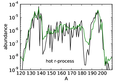
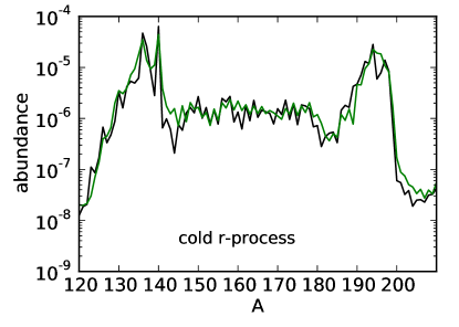
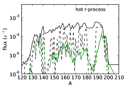
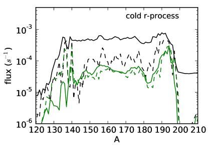
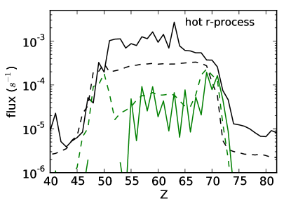
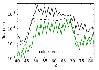
Figure 8: (Color online) Abundances and fluxes (Eqs. 4–5) vs. A and Z are shown for the hot (left column) and cold (right column) r-process. The black lines correspond to freeze out ($Y_{n}/Y_{\mathrm{seed}}=1$) and the green lines to the time when $\tau_{\beta}=\tau_{(n,\gamma)}$. The beta decay flux is represent by dashed lines and the net neutron capture flux by solid lines.

The competition between beta decay (with delayed-neutron emission) and neutron capture when matter decays to stability is important to understand the differences in the final abundances between the hot and cold r-process. Let us consider a nucleus with charge $Z$ and mass number $A$. Its abundance can change by beta-decay, neutron capture, and photodissociation. The competition among these processes can be quantified by the beta decay flux:

$$F_{\beta}(Z,A)=\lambda_{\beta}(Z,A)Y(Z,A)\,,$$ (4)

and by the net neutron capture flux:

$$F_{n}(Z,A)=Y(Z,A)N_{n}\langle\sigma v\rangle_{Z,A}-\lambda_{\gamma}(Z,A+1)Y(Z,A+1).$$ (5)

In order to visualize these quantities, it is convenient to define the fluxes for an isotopic chain, $F_{\beta}(Z)=\sum_{A}F_{\beta}(Z,A)$ and $F_{n}(Z)=\sum_{A}F_{n}(Z,A)$, and the fluxes for an isobaric chain, $F_{\beta}(A)=\sum_{Z}F_{\beta}(Z,A)$ and $F_{n}(A)=\sum_{Z}F_{n}(Z,A)$. As discussed in the Appendix, we expect that for the hot r-process a beta-flow equilibrium is achieved Kratz et al. (1993). This implies that the $F_{\beta}(Z)$ reaches a constant value independent of $Z$. In the cold r-process one expects that both $F_{\beta}(Z)$ and $F_{n}(A)$ become constant. This is confirmed in Fig. 8 that shows the net neutron capture and beta-decay fluxes versus mass number (middle panels) and versus proton number (bottom panels). Notice, that in the s-process Käppeler (1999) $F_{n}(A)$ is also constant and there are strong odd-even effects in the abundances. This is due to the large odd-even effects present in the neutron capture rates and the fact that beta-decay can be assumed instantaneous compared to s-process timescales. In contrast, in our case these strong odd-even effects are not present because beta-decay rates become similar to neutron-capture rates as matter decays to stability.

The fluxes $F_{n}(A)$ and $F_{\beta}(A)$ present several features when $\tau_{\beta}=\tau_{(n,\gamma)}$ that can explain how matter is redistributed. In the regions where beta-decay dominates over neutron captures, nuclei will beta decay without substantially changing the mass number, e.g., see Fig. 8 for $A>195$. On the other hand, nuclei in regions where neutron capture dominates over beta-decay will predominantly capture neutrons and consequently the abundances will shift to higher mass numbers, as shown in Fig. 8 for $A=182$–195. The formation of the rare-earth peak (not yet present in the abundances shown in upper panels of Fig. 8) is also due to neutron capture as matter decays to stability. In the region $A=162$–168 the beta-decay and neutron-capture fluxes are very similar, while in the region $A<162$ the latter dominates (Fig. 8). This produces a net movement of matter from nuclei with $A<162$ to nuclei with $A\approx 162$ that will result in the formation of the rare-earth peak. The formation of this peak has to wait until the moment when the beta decay fluxes become larger than the neutron capture fluxes in that region. The reason why the neutron capture fluxes can become locally smaller for these nuclei (when compared with slightly heavier or lighter nuclei) is the presence of a deformed sub-shell closure around $A\approx 162$ (see Fig. 6) that results in a sudden drop of neutron-capture rates.

In the hot r-process, the fluxes (Fig. 8, right column) present more fluctuations due to photodissociation reactions. These reactions can result in negative net neutron capture fluxes in regions where the photodissociation is still important. This leads to an extra supply of neutrons that can be important at later times. Negative net neutron capture fluxes appear in the hot r-process for $A\lesssim 145$ and $Z\lesssim 53$ once $\tau_{\beta}=\tau_{(n,\gamma)}$. They are not shown in Fig. 8 as we use a logarithmic scale.

III.3.1 The role of neutron capture

In order to explore the impact of neutron capture we compare two different sets of rates based both on the FRDM mass model. The first set corresponds to statistical model calculations of Ref. Rauscher and Thielemann (2000) and it was used in previous sections. The second set is computed with the analytic approximation suggested in Ref. Michaud and Fowler (1970). These two sets of neutron-capture rates are compared in Fig. 9 for three different isotopic chains in regions relevant for the r-process. The Ru isotopes are populated in the region $N\lesssim 82$, Xe isotopes for $N\sim 100$, and Er isotopes for $N\lesssim 126$. The largest differences between both sets of neutron-capture rates occur for nuclei just before neutron shell closures. For these nuclei the level density around neutron separation energy becomes rather low and consequently the rates are very sensitive to the treatment of parity Loens et al. (2008) and to the dipole strength distribution Litvinova et al. (2009). In addition, the statistical model may not be applicable for some of these nuclei at r-process temperatures (see Fig. 7 of Ref. Rauscher et al. (1997)) and direct capture should be included Mathews et al. (1983); Goriely (1997).

Figure 9: (Color online) Neutron-capture rates as computed in Ref. Rauscher and Thielemann (2000) (solid lines and filled symbols) compared to rates based on the analytical approximation of Ref. Michaud and Fowler (1970) (dashed lines and empty symbols). The rates are shown for 3 different isotopic chains in the region of relevance for r-process nucleosynthesis.

The abundances based on the two sets of neutron-capture rates are shown in Fig. 10 for the hot and cold r-process. At freeze-out both sets of neutron-capture rates leads to very similar abundances. In the hot r-process, the abundances are independent of the neutron-capture rates since the evolution proceeds under $(n,\gamma)\rightleftarrows(\gamma,n)$ equilibrium (see Appendix). The cold r-process is characterized by the competition between neutron capture and beta decay, however only small changes are present in the freeze-out abundances when the neutron-capture rates are varied. Notice that the position and the height of the peaks are the same. In contrast, the final abundances exhibit significant differences: The third r-process peak is more shifted towards higher mass number and the abundances between peaks are less smooth for the calculations based on the approximate neutron-capture rates.

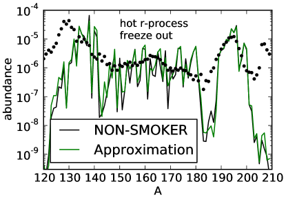
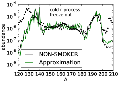
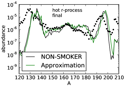
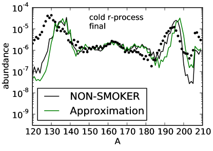
Figure 10: (Color online) Abundances at freeze-out (upper panels) and after decay to stability (bottom panels) for the hot (left panels) and cold (right panels) r-process. The abundances are obtained using two different sets of neutron-capture rates both based in the same nuclear mass model (FRDM Möller et al. (1995)). The first set of neutron-capture rates, labeled NON-SMOKER (black lines), corresponds to the calculations of Ref. Rauscher and Thielemann (2000). The second set, labeled as “Approximation” (green lines), has been obtained using the analytical approximation derived in Ref. Michaud and Fowler (1970).

The competition of the nuclei to capture the few neutrons available can be quantified by the net probability of a nucleus for neutron capture, that we define as

$$P_{n,\gamma}(Z,A)=\frac{F_{n}(Z,A)}{\sum_{Z,A}F_{n}(Z,A)}\,,$$ (6)

using net neutron capture flux, $F_{n}(Z,A)$, introduced in Eq. (5). The denominator in this expression represents the change of neutron abundance due to neutron captures and photodissociations and it is always positive since the neutron abundance continuously decreases during an r-process calculation. The numerator is positive for the majority of nuclei, although can become negative for some of them. The change in abundances after freeze-out is thus more pronounced in regions with larger $P_{n,\gamma}(Z,A)$.

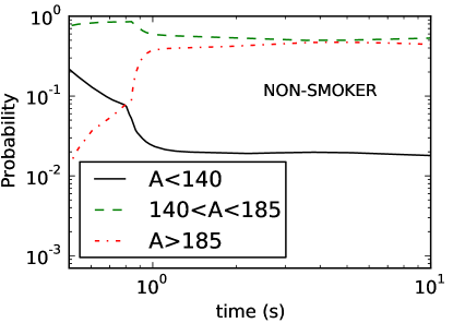
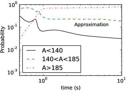
Figure 11: (Color online) Probability of neutron capture (Eq. (6)) vs. time for different mass number intervals based on NON-SMOKER rates (left panel) and on the approximated rates (right panel).

Figure 11 shows the neutron-capture probability for different regions: around the second r-process peak ($A<140$), between peaks ($140\leq A<185$), and around the third peak ($A\geq 185$) for the hot r-process. The results are qualitatively the same for the cold r-process. As expected from the agreement between the freeze-out abundances, the initial evolution of the probabilities is rather similar and follows the build up of increasingly heavier nuclei during the r-process. At early times most of the captures takes place in the region around and below the second r-process peak. Later as nuclei in the region between peaks are produced, the neutrons are mainly captured in this region. Just before freeze-out ($t\approx 1$ s), there is an increase in the capture probability around the third peak. The evolution after freeze-out strongly depends on the neutron captures. In the calculation with NON-SMOKER rates (Fig. 11, left panel), the neutron-capture probability is similar for the regions around the third peak and between peaks, with the latter dominating slightly. This is in contrast to the neutron-capture probability based on the approximate rates (Fig. 11, right panel) which is clearly higher in the region of the third peak than in the region between peaks. Therefore, neutrons are mainly captured around the third peak. This leads to the shift of the peak towards even higher $A$ than with the NON-SMOKER rates and leaves pronounced odd-even features between peaks. Consequently, when the approximate rates are used, beta-delayed neutron emission is the only mechanism to smooth the abundances between $A=130$ and $A=195$ after freeze out. While using the NON-SMOKER rates, both (neutron capture and beta-delayed neutron emission) contribute to produce a smother r-process distribution.

Our results demonstrate that neutron-capture rates are key for the determination of the final r-process abundances, specially around the third peak and between peaks where a robust pattern is found in old metal-poor halo stars and solar system (see e.g., Ref. Sneden et al. (2008)). Similar conclusions were reached in Ref. Rauscher (2005) where individual neutron-capture rates were changed by an arbitrary factor. However, our results illustrate more clearly the non-local character of the competition for the few available neutrons which can produce global changes in the r-process abundances. In addition to the variation of the third-peak position, we find also substantial changes in the abundances around $A\sim 150$, even if both regions are not directly connected by any reaction. Similar global changes were obtained in Refs. Surman et al. (2009); Beun et al. (2009b); Farouqi et al. (2010) where the sensitivity of the r-process abundances to changes of the neutron-capture rates around $A=130$ was studied.

III.3.2 Beta-delayed neutron emission

After we have shown the importance of beta decay when matter decays to stability, it is worth to analyze the effect of beta-delayed neutron emission. In the classical r-process, where no neutron captures are considered after freeze out, beta-delayed neutron emission is the only way to redistribute matter and get smooth final abundances. In Fig. 12 we explore the effect of beta-delayed neutron emission in the hot (left column) and cold (right column) r-process. The black lines correspond to the standard network calculations with beta-delayed neutron emission included and the green lines to calculations where beta-decay takes place without emitting neutrons, i.e. $A$ is conserved. The effect of beta-delayed neutron emission and its subsequent capture was also investigated for different long-time dynamical evolutions in Wanajo et al. (2002); Farouqi et al. (2010).

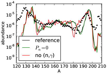
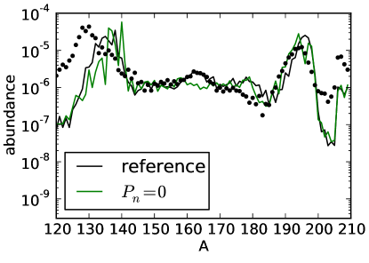
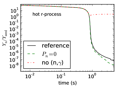
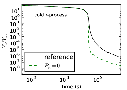
Figure 12: (Color online) Effect of the beta-delayed neutron emission in the hot (left column) and cold (right column) r-process, using neutron captures and beta decays based on the FRDM mass model. The black lines are for the reference case calculated with the standard nuclear input: neutrons are emitted with given probability ($P_{n}$) after beta decay. The green lines are for the case $P_{n}=0$, i.e. A is conserved during beta decay. For the red dash-dotted line the neutron captures and the photodissociation reactions are suppressed after freeze-out.

After freeze-out, more neutrons are present when beta-delayed neutron emission is considered and thus the neutron-to-seed ratio is higher as shown in the bottom panels of Fig. 12. However, in our hot r-process such differences are too small to have an impact on the final abundances. In this case, photodissociation produces also neutrons in addition to beta decay. Our results seem to contradict classical r-process calculations, where the redistribution of matter is due only to beta-delayed neutron emission. One should notice that our freeze-out path is in agreement with classical r-process calculations (see e.g. Kratz et al. (1993)). Moreover, if we neglect all neutron captures after freeze-out (as it is done in the classical r-process) and only consider beta-delayed neutron emission, we obtain the abundances shown by the red line in Fig. 12. This calculation reproduces the position and width of the third peak but present larger oscillations in the final abundances. Similar results were also found in the classical r-process calculations of Ref. Kratz et al. (1993) demonstrating that beta-delayed neutron emission cannot completely remove the fluctuations in the freeze-out abundances. Once neutron captures are considered the abundance distribution becomes smoother like in the solar system and the rare-earth peak forms (black line in the upper panels of Fig. 12). However, the third peak becomes narrower and shifts to mass number values larger than $A\sim 195$.

In our cold r-process, the beta-delayed neutron emission has more impact on the final abundances (Fig. 12). Since photodissociation is negligible, the r-process path can move farther away from stability reaching nuclei with higher probability of emitting neutrons after beta-decay. This leads to significant differences in the neutron-to-seed ratio shown in the bottom panel of Fig. 12. The freeze-out is more instantaneous without beta-delayed neutron emission and this has two main effects: the third peak is less shifted and the rare earth peak is not produced. Therefore, we can conclude that beta-delayed neutron emission is very important to supply the neutrons that through several captures will determine the final abundances. Moreover, the freeze-out cannot be totally instantaneous because neutron capture are required to form the rare earth peak at late times.

III.3.3 Non-instantaneous freeze-out

Finally, we want to discuss a general feature present in the evolution of the neutron-to-seed ratio. After an initial slow decrease, the neutron-to-seed reaches a phase of fast decline once its value becomes around one. However, this fast decline, that will correspond to an instantaneous freeze-out as assumed in classical r-process calculations, is always interrupted and the neutron-to-seed ratio follows a more moderate decrease afterward. This is a generic feature found in all dynamical calculations (see e.g. Refs. Meyer et al. (1992); Howard et al. (1993); Woosley et al. (1994)) and indicates that the freeze-out effects discussed here will always be important. We found that the sudden change in the evolution of the neutron-to-seed ratio, mathematically corresponding to the appearance of an inflexion point, occurs when the average neutron-capture rate (Eq. (2a)) and the average beta-decay rate (Eq. (2c)) are identical, i.e. $\tau_{(n,\gamma)}=\tau_{\beta}$. Interestingly, this happens even in the calculations where beta-delayed neutron emission is artificially switched off, see Fig. 12. This phase of moderate decline of the neutron-to-seed ratio is the so-called s-process phase of the r-process Meyer (1993) in which beta-decay dominates over neutron-capture. During this phase, the rare-earth peak is formed in our calculations based on the FRDM mass model. However, in these calculations the third r-process peak is shifted to mass number values larger than $A\sim 195$.

IV Summary and conclusions

We have studied the impact of the long-time dynamical evolution and nuclear physics input on the r-process abundances. Our calculations are based on hydrodynamical trajectories from core-collapse supernova simulations of Ref. Arcones et al. (2007) with the entropy increased by a factor two (i.e., density decreased by a factor two) in order to produce the third r-process peak. We have chosen two different evolutions to cover the two possible physical conditions at which the r-process occurs in high entropy ejecta. These evolutions are identical during the seed formation phase and differ only after the temperature becomes $\lesssim 3$ GK and the nucleosynthesis flow is dominated by neutron captures, i.e. the r-process phase. This guarantees that changes in the resulting abundances are due to the modification of the long-term evolution and/or the nuclear physics input and not to changes in the initial conditions. The long-time evolution is varied assuming that the reverse shock is at different temperatures, which is justified based on two-dimensional simulations Arcones and Janka (2010). The two typical long-time evolutions are:

• hot r-process that occurs when the reverse shock is at high enough temperatures ($T\gtrsim 0.5$ GK) to reach an $(n,\gamma)\rightleftarrows(\gamma,n)$ equilibrium that lasts until neutrons are exhausted.

• cold r-process (with the reverse shock at low temperatures) that takes place under a competition between neutron capture and beta decay.

The main difference between these evolutions is that in the cold r-process the photodissociation is negligible Wanajo (2007). Therefore, the r-process path can move farther away from stability reaching nuclei with shorter beta-decay half-lives and leading to a faster evolution and an earlier freeze out than in the hot r-process.

We can distinguish two phases during the r-process that are characterized by different nuclear physics processes. Before freeze-out, $Y_{n}/Y_{\text{seed}}>1$, the most relevant nuclear physics input depends on the type of r-process taking place, hot or cold r-process:

• In the hot r-process the most relevant input are the nuclear masses as they determine the r-process path via the neutron separation energy. A very good approximation to the freeze-out abundances of the hot r-process is obtained assuming that matter achieves steady beta-flow, i.e. $\lambda_{\beta}(Z)Y(Z)=\text{constant}$ (see Eq. (13)). It is well known Burbidge et al. (1957); Cameron (1957) that in this case the peaks in the r-process abundance distribution at $A=130$ and $A=195$ are associated with long beta-decay half-lives at the magic neutron numbers $N=82$ and $N=126$ where the r-process path is closer to the stability.

  The abundances at freeze-out in the hot r-process are characterized by the presence of large troughs that occur in regions where the two neutron separation energy is almost constant or presents a saddle point. This typically occurs before (after) a magic neutron number where a transition from deformed (spherical) to spherical (deformed) shapes takes place. As experimental data for two neutron separation energies do not show this behavior Audi et al. (2003), this may indicate a drawback in some of the mass models used. However, the solar abundances suggest a small trough in the region before the third peak, $A=180$–190, that could be related with a transition from deformed to spherical nuclei.

• In the cold r-process the most relevant inputs are beta-decay and neutron-capture rates. The nuclei at the r-process path are those with similar neutron-capture and beta-decay rates for a given neutron density. Our results are the first to show that the abundances at freeze-out achieve steady flow for both beta decays and neutron captures, i.e. $\lambda_{\beta}(Z)Y(Z)$ and $\langle\sigma v\rangle_{A}Y(A)$ are constant (see Eq. (14)). This suggests that the cold r-process is more robust than the hot r-process, as the abundances fulfil additional constraints.

The sensitivity of the mass model has been investigated by consistently using neutron separation energies and neutron capture rates based on the mass models: FRDM, ETFSI-Q, HFB-17, and Duflo-Zuker. Our results show peculiarities coming from each mass model. In ETFSI-Q the quenching of the $N=82$ shell closure leads to a slow down of the evolution and to a later freeze-out. Moreover, the large values of $S_{2n}$ before $N=126$ in this mass model make the trough in the freeze-out abundances for $A\approx 185$ bigger due to neutron captures when matter decays to stability. Results based on FRDM are clearly affected by the anomalous behaviour of $S_{2n}$ before $N=90$, which produces the accumulation of matter and thus the formation of peaks around $A\approx 135$ even in the cold r-process.

In order to study the evolution after freeze-out we have used the fluxes for neutron captures and beta decays. They help us to explain the final features in the abundances, such as the exact position of the r-process peaks and the formation of the rare earth peak. These are our most significance outcomes:

• The abundances at freeze-out can be approximated assuming a steady beta-flow (hot r-process) or a steady flow of beta decays and neutron captures (cold r-process) for a given neutron density and temperature. However, the final abundances are determined by the evolution after freeze-out. In all cases considered, the final abundances are substantially different and smother than the freeze-out abundances. Most of the smoothing takes place just after freeze-out when the timescale for neutron captures is still shorter than the one for beta-decays, $\tau_{(n,\gamma)}<\tau_{\beta}$, see Eq. (2). Hence, neutron captures play a dominant role in producing a smooth distribution. Nevertheless, the evolution once $\tau_{(n,\gamma)}>\tau_{\beta}$ is also important. During this phase the decrease of the neutron-to-seed ratio is rather moderate and determined by the timescale at which matter beta decays to stability, even in calculations where beta-delayed neutron emission is artificially suppressed.

• The impact of the neutron capture rates has been investigated by comparing results based on the same mass model (FRDM) but different sets of neutron-capture rates: A set is based in statistical model calculations with the code NON-SMOKER Rauscher and Thielemann (2000) and the other in the analytical approximation derived in Ref. Michaud and Fowler (1970). We find that the abundances at freeze-out for hot and cold r-process are rather similar for both sets of neutron capture rates. However, after freeze-out we find that most of the neutrons are captured in the region between r-process peaks when using the NON-SMOKER rates. In contrast, with the approximated rates neutrons are captured more probably in the region around the third peak. The end result is a larger shift of the third peak and a less smooth abundance distribution between peaks with the approximated rates than with the NON-SMOKER rates. This emphasizes the important role of neutron captures after freeze-out.

• The small rare-earth peak, observed around $A\sim 160$ in the solar r-process distribution, must necessarily be formed after the freeze-out, since it is not present in any of the freeze-out abundances. Furthermore, it is also not present in the abundances when $\tau_{(n,\gamma)}\approx\tau_{\beta}$. We find, see also Refs. Surman et al. (1997); Surman and Engel (2001), that the rare-earth peak forms by neutron captures when matter decays to stability.

• The main role of beta-delayed neutron emission is the supply of neutrons. In the hot r-process we find no difference in the abundances calculated with and without beta-delayed neutron emission. Since temperature is high, photodissociation prevents the path from reaching regions far from stability where the probability of emitting neutrons after beta decay is large. Furthermore, photodissociation reactions are also a source of neutrons. In contrast, in the cold r-process the neutron-to-seed ratio reaches significantly smaller values when beta-delayed neutron emission is suppressed. This leads to a reduction in the shift of the third peak after freeze out but also inhibits the formation of the rare earth peak. This confirms the argument given above that the peak forms by neutron captures.

Our results clearly rise the importance of future experiments to measure nuclear masses, neutron capture rates and beta-decay half-lives for nuclei far from stability. This will provide not only direct input for network calculations, but also important constraints for the theoretical nuclear models. We have shown that the r-process abundances are very sensitive to the set of neutron capture rates as they determine the regions in which neutrons are capture predominantly. More experimental effort is necessary for an improved determination of neutron capture cross sections. Since these experiments are difficult, sensitivity studies to determine the most relevant neutron capture rates will be necessary. Our results show a strong interplay between the late-time evolution of the ejected matter and the nuclear physics input. This could constrain the astrophysical conditions once future radioactive experimental facilities deliver high quality experimental data for r-process nuclei.

*

Appendix A Formalism

During the r-process, and assuming that charged particle reactions, fission and alpha decays can be neglected, the evolution of the abundances is mainly determined by neutron capture, photodissociation, and beta-decays. This results in the following differential equation that determines the change of the abundance of a nucleus with charge $Z$ and mass number $A$:

$$\frac{dY(Z,A)}{dt} = \rho N_{A}\langle\sigma v\rangle_{Z,A-1}Y_{n}Y(Z,A-1)+\lambda_{\gamma}(Z,A+1)Y(Z,A+1)$$ (7)

$$+\sum_{j=0}^{J}\lambda_{\beta jn}(Z-1,A+j)Y(Z-1,A+j)$$

$$-\left(\rho N_{A}\langle\sigma v\rangle_{Z,A}Y_{n}+\lambda_{\gamma}(Z,A)+\sum_{j=0}^{J}\lambda_{\beta jn}(Z,A)\right)Y(Z,A)$$

where $Y_{n}$ is the neutron abundance, $\langle\sigma v(Z,A)\rangle$ is the thermal averaged neutron-capture rate, and $\lambda_{\gamma}(Z,A)$ the photodissociation rate for a nucleus ${}^{A}Z$, while $\lambda_{\beta jn}(Z,A)$ is the $\beta^{-}$ decay rate of ${}^{A}Z$ with emission of $j$ delayed neutrons (up to a maximum of $J$). The photodissociation rate is related to the neutron capture rate by detailed balance:

$$\lambda_{\gamma}(Z,A+1)=\langle\sigma v\rangle_{Z,A}\left(\frac{m_{u}kT}{2\pi\hbar^{2}}\right)^{3/2}\frac{2G(Z,A)}{G(Z,A+1)}\left(\frac{A}{A+1}\right)^{3/2}\exp\left[-\frac{S_{n}(Z,A+1)}{kT}\right],$$ (8)

where $G$ is the particition function and $S_{n}=m_{n}+M(Z,A-1)-M(Z,A)$ is the neutron separation energy with $m_{n}$ the neutron mass and $M(Z,A)$ the mass of the nucleus.

If the assumption is made that the neutron abundance varies slowly enough, it can be assumed that the neutron density, $N_{n}=Y_{n}\rho N_{A}$, is constant over a timestep. In this case the network can be divided into separate pieces for each isotopic chain and solve then sequentially, beginning with the lowest $Z$ Cowan et al. (1983). However, this approximation becomes numerically unstable when the neutron abundance becomes small, $Y_{n}\lesssim 10^{-5}$. Consequently, it is better to include in the set of differential equations the one determining the change of the neutron abundance:

$$\frac{dY_{n}}{dt}= - \sum_{Z,A}\rho N_{A}\langle\sigma v\rangle_{Z,A}Y_{n}Y(Z,A)$$ (9)

$$+ \sum_{Z,A}\lambda_{\gamma}(Z,A)Y(Z,A)$$

$$+ \sum_{Z,A}\left(\sum_{j=1}^{J}j\lambda_{\beta jn}(Z,A)\right)Y(Z,A)$$

The system of differential equations defined by Eq. (7) and (9) allows for several approximations that are valid in different physical regimes. A commonly used assumption in classical r-process calculations is the $(n,\gamma)\rightleftarrows(\gamma,n)$ equilibrium. This approximation is valid whenever the neutron density ($N_{n}\gtrsim 10^{20}$ cm^-3) and temperature ($T\gtrsim 1$ GK) Cameron et al. (1983) are large enough to warrant that both the rate of neutron capture ($N_{n}\langle\sigma v\rangle$ and the photodissociation rate ($\lambda_{\gamma}$) are much larger than the beta decay rate ($\lambda_{\beta}$) for all the nuclei participating in the network. Under this conditions the evolution of the system is mainly determined by the beta decay rates as the abundances along an isotopic chain are inmediatly adjusted to an equilibrium between neutron captures and photodissociations, i.e. $N_{n}Y(Z,A)\langle\sigma v\rangle_{Z,A}=\lambda_{\gamma}(Z,A+1)Y(Z,A+1)$. Combining these result with Eq. (8) one obtains that the abundances in an isotopic chain are given by the simple relation:

$$\frac{Y(Z,A+1)}{Y(Z,A)}=N_{n}\left(\frac{2\pi\hbar^{2}}{m_{u}kT}\right)^{3/2}\left(\frac{A+1}{A}\right)^{3/2}\frac{G(Z,A+1)}{2G(Z,A)}\exp\left[\frac{S_{n}(Z,A+1)}{kT}\right].$$ (10)

For each isotopic chain, the above equation defines a nucleus that has the maximum abundance and which is normally known as waiting point nucleus as the flow of neutron captures “waits” for this nucleus to beta-decay. The set of waiting point nuclei constitutes the r-process path. The maximum of the abundance distribution can be determined setting the left-hand side of Eq. (10) to 1, which results in a value of $S_{n}$ that is the same for all isotopic chains for a given neutron density and temperature:

$$S^{0}_{n}(\text{MeV})=\frac{T_{9}}{5.04}\left(34.075-\log N_{n}+\frac{3}{2}\log T_{9}\right),$$ (11)

where $T_{9}$ is the temperature in units of $10^{9}$ K and $N_{n}$ is the neutron density in cm^-3. Equation (11) implies that the r-process proceeds along lines of constant neutron separation energies towards heavy nuclei. For typical r-process conditions this corresponds to $S^{0}_{n}\sim 2$–3 MeV. Due to pairing, the most abundance isotopes have always an even neutron number. For this reason, it may be more appropriate to characterize the most abundance isotope in an isotopic chain as having a two-neutron separation energy $S_{2n}=2S^{0}_{n}$ Goriely and Arnould (1996). The two-neutron separation energy is not a continuous function of neutron number but shows large jumps particularly close to magic neutron numbers. For this reason r-process nuclei near to magic numbers have neutron separation energies much larger than the typical 2–3 MeV and the r-process path moves closer to the stability (see figure 6).

If $(n,\gamma)\rightleftarrows(\gamma,n)$ equilibrium is valid it is sufficient to consider the time evolution of the total abundance of an isotopic chain $Y(Z)=\sum_{A}Y(Z,A)$ as the abundances of different isotopes are fully determined by Eq. (10). From Eq. (7) we can determine the time evolution of $Y(Z)$ obtaining:

$$\frac{dY(Z)}{dt}=\lambda_{\beta}(Z-1)Y(Z-1)-\lambda_{\beta}(Z)Y(Z)$$ (12)

where $\lambda_{\beta}(Z)=\sum_{A}\lambda_{\beta}(Z,A)Y(Z,A)/Y(Z)$. In this case the r-process evolution is independent of the neutron-capture rates, only beta-decays are necessary for Eq. (12) and masses via $S_{n}$ in Eq. (10). If the r-process proceeds in $(n,\gamma)\rightleftarrows(\gamma,n)$ equilibrium and its duration is larger than the beta decay lifetimes of the nuclei present, Eq. (12) tries to reach an equilibrium denoted as steady $\beta$-flow Kratz et al. (1993) that satisfies for each $Z$ value:

$$\lambda_{\beta}(Z-1)Y(Z-1)=\lambda_{\beta}(Z)Y(Z)$$ (13)

In this case the peaks at $A=130$ and 195 in the solar r-process distribution can be attributed to the long $\beta$-decay lifetimes of the waiting point nuclei with $N=82$ and 126, where the r-process path gets closer to the stability (see figure 6). This is the case for the equilibrium calculations discussed in the text before freeze-out of neutron captures.

The r-process can also operate under such a low temperatures that the photodissociation rates in Eq. (7) can be neglected. Under this conditions the r-process operates under a competition of neutron captures and beta decays. If one neglects beta-delayed neutron emission, Eq. (7) can be reduced to two independent equations that govern the evolution of the total abundance along an isotopic chain, $Y(Z)$ and along an isobaric chain, $Y(A)=\sum_{Z}Y(Z,A)$:

$$\frac{dY(Z)}{dt}=\lambda_{\beta}(Z-1)Y(Z-1)-\lambda_{\beta}(Z)Y(Z)$$ (14a)

$$\frac{dY(A)}{dt}=N_{n}\langle\sigma v\rangle_{A-1}Y(A-1)-N_{n}\langle\sigma v\rangle_{A}Y(A)$$ (14b)

were $\langle\sigma v\rangle_{A}=\sum_{Z}\langle\sigma v\rangle_{Z,A}Y(Z,A)/Y(A)$. If the r-process duration is longer than the beta-decay and neutron capture lifetimes, Eq. (14) reaches an equilibrium that we will denote as steady flow that satisfies for each $Z$ and $A$:

$$\lambda_{\beta}(Z-1)Y(Z-1)=\lambda_{\beta}(Z)Y(Z)$$ (15a)

$$\langle\sigma v\rangle_{A-1}Y(A-1)=\langle\sigma v\rangle_{A}Y(A)$$ (15b)

In addition, as the r-process occurs under a competition of beta-decays and neutron captures one obtains that $N_{n}\langle\sigma v\rangle_{A}Y(A)\approx\lambda_{\beta}(Z)Y(Z)$. As the abundances along an isotopic and isobaric chain are dominated by a single nucleus this condition determines also the nuclei that participate in the r-process, i.e. the r-process path. Similarly to what happens in the equilibrium case, the peaks in the abundance distribution correspond to long beta decay lifetimes. However, in this case the peaks are in addition associated with long neutron capture lifetimes.