Gamma-ray variability and correlation properties of blazars observed with Fermi LAT

Abstract

The Fermi Large Area Telescope (Fermi LAT) provides long term systematic monitoring observations of the gamma-ray emission from blazars. The variability properties and the correlation with other wavelength bands are important clues for the evaluation of blazar models. We present results from timing and multiwavelength correlation analysis and discuss differences between blazar classes.

1 Introduction

More than 60 AGNs, almost all blazars, were detected by EGRET on Compton GRO, which established these sources as a powerful class of gamma-ray emitters [1]. In its first year of operation Fermi LAT has increased the number of known gamma-ray blazars by a factor of 10. Even more importantly the instrument is mapping the full sky every three hours, which allow regular monitoring of these sources on time scales from hours to years. These monitoring observations now form an important part of many ongoing efforts to study the variability and multiwavelength properties of blazars. Such observations contains information about the relative origin of different spectral components and about dynamical and radiation processes in blazar jets.

2 The Fermi Large Area Telescope

Fermi (the Fermi Gamma-ray Space Telescope) was launched in June 2008 from Cape Canaveral in Florida. The main instrument onboard Fermi is the LAT (Large Area Telescope) which is sensitive to gamma-rays in the energy range 30 MeV to 300 GeV [2]. With a much larger field of view and with a much improved energy resolution compared to its predecessors, Fermi is now providing unprecedented data for studies of active galactic nuclei and other gamma-ray sources. Fermi is operated primarily in a sky survey mode where the full sky is mapped every three hours. Since LAT has a very wide field of view (about 20% of the sky) the exposure on any particular sky position is large. Pointed observations are executed only to follow up GRBs or during other exceptional outbursts. The sky surveying and wide field of view of the instrument also mean that the potential for new, serendipitous discoveries is very large. The angular resolution, which increases with photon energy, is about 1 degree at 1 GeV, while source localizations are typically 0.1 degrees.

3 LBAS, 1LAC and 2LAC

Based on the first 3 months of observations a LAT bright-AGN Source list (LBAS) was produced by the Fermi LAT collaboration [3]. This list contains 106 high confidence associations (58 FSRQs, 42 BL Lacs, 2 radio galaxies and 4 of unknown type). These were sources with detection test statistic, TS $>$ 100, corresponding approximately to $10\sigma$ detections. By comparison, the First LAT AGN catalog, 1LAC [4] based on 11 months of data included already 663 high confidence associations (sources with TS $>$ 25, or approximately $5\sigma$ ). In the recently released second AGN catalog, 2LAC, this number of sources was increased by 50$\%$[5].

4 Blazar variability

Blazar light curves are often dominated by strong flares. The origin of these flares can e.g. be the bulk injection of new particles into the jet or strong internal shocks. If the variability is made up of shot pulses of different lengths and amplitudes produced by such events, the Power Density Spectrum (PDS) is determined by the shapes and amplitudes of the pulses and by correlations of their relative distribution in time. While pulse shapes might be associated with, e.g., cooling or light travel time scales, pulse correlations will contain information on the processes that are responsible for creating the pulses, which could be episodes of strong activity near the central black hole. By calculating the PDS, the Structure Function (SF), and other statistical mesures, we can test alternative mechanisms to produce the observed variability, keeping in mind that the same PDS or SF can be produced by more than one stochastic process.

The Fermi LAT data can be used to study variability on time scales of hours to years, to measure spectral variations and to catch flaring sources with high efficiency. An example of the capability to study flux and spectral variations on subday time scales is given by the analysis of the recent outburst of 3C454.3 [6].

For timing analysis the regular sampling provided by Fermi LAT is a great advantage. The initial aim of our study of Fermi blazars is a characterization the gamma-ray variability. The tools that have been used for this are,

• $\chi^{2}$ and excess variance to quantify the presence of variability and its significance.

• Duty cycle analysis

• Auto correlation function (ACF)

• Structure function (SF)

• Power Density Spectra (PDS)

• Flare shape analysis

Even though the ACF, SF and PDS contain the same information, this information is expressed differently, which makes it useful to compute all three. The direct fitting of flare shapes is based on the assumption that individual flare pulses can be identified. The advantage with this approach is the possibility to extract light curve phase information, which is lost in the calculations of ACF/SF/PDS. This includes e.g. time asymmetry.

First results of our work, using 11 months of data and light curves with 3 to 7 days binning for the LBAS sources was recently published [7] and is partly summarized here.

4.1 Power Density Spectra

Power Density Spectra (PDS) of blazars have previously been studied primarily for optical and radio data and have then in general been described by a power law $P(\nu)\propto\nu^{-\alpha}$ with $\alpha$ typically in the range 1 to 2.

For the PDS analysis of Fermi blazars, light curves with 3 day binning was used for the 15 brightest LBAS sources (9 FSRQs and 6 BL Lacs). For a further 13 FSRQs with slightly lower flux, the binning was increased to 4 days. A standard Fourier transform was used to compute power density spectra (PDS) and the white noise level corresponding to the estimated measurement errors was subtracted.

The power spectral density is normalized to fractional variance per frequency unit ( rms² I^-2 Day^-1, where $~{}I$ is the mean flux) and the PDS points are averaged in logarithmic frequency bins. An example PDS for 3C273 is shown in Figure 1 and the 1-week-binned light curve for the same source is presented in Figure 2.

Figure 1: PDS of the 11 month Fermi light curve for 3C273. A 3 day binned light curve was used. The PDS is normalized to variance divided with the square of the mean flux and per frequency unit (from [7]).

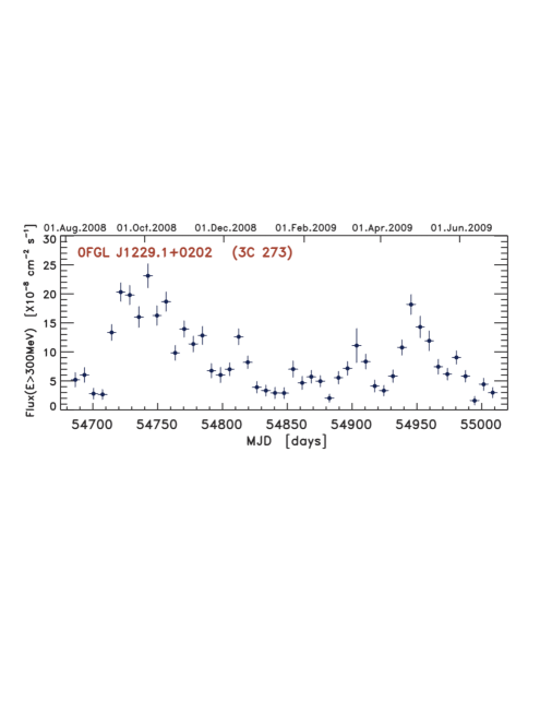
Figure 2: Fermi 11 month light curve (1 week binning) for 3C273 (from [7]).

There are a number of effects that can distort the shape of the computed PDS and cause it to differ from the ’true’ intrinsic PDS describing the variability of the source. These effects are,

• Stochastic variability in a time limited observation.

• Effects of the observational data and the analysis (e.g. aliasing).

• Systematic errors

• Statistical (measurement) errors.

For the analysis presented here the last effect dominates at high frequencies and the first effect at the lower frequencies where source variance is much larger than the measurement noise. The white noise level used in the analysis has a significant effect on the slope deduced from the PDS fit. This means that the result is dependent of a reliable estimate of the measurement errors. These errors were therefore also checked by comparing some light curves with the corresponding ones obtained by direct aperture photometry, for which Poisson statistics is valid. This showed that the uncertainty in error estimates is not a significant problem for the brightest sources. For the less bright ones, including all the BL Lacs, this effect may however, introduce a systematic bias in the PDS slope. The effect was estimated by repeating the analysis for a range of possible white noise levels and also by analysis of light curves extracted with different time bins (from 1 to 7 days). To limit the effect of the white noise on the determination of the PDS slope, the fits only used frequencies up to 0.02  day^-1.

Observational and instrument systematics were investigated by analyzing pulsar light curves extracted from the 11 month data with the same procedure as for the blazars. The most prominent effect is a periodic modulation that is identified with the 54 day precession period of the Fermi satellite orbit. In the PDS for individual blazars this peak is often hidden by the stochastic variability but does show up when averaging the PDS of a number of sources. The frequency bin at this period was not used when PDS slopes were estimated.

With the available data the uncertainty in PDS shape for individual sources is still dominated by stochastic variability. To reduce this and the statistical fluctuations we can average the PDS for a group of sources under the assumption that the differences in PDS shape is small compared to the random fluctuations expected due to the action of the (presumed) underlying stochastic process. For the 9 brightest FSRQs this averaged PDS is shown in Figure 3. For frequencies below 0.017 we obtain a best fit slope of 1.4 $\pm$0.1. The same PDS is also shown in Figure 4 together with the corresponding averaged PDS for the 9 BL Lacs and the 13 moderately bright FSRQs. The differences in power-law slope are not statistically significant (errors are estimated from the scatter within each group of sources).

Figure 3: Average Power Density spectrum, PDS, for the 9 brightest FSRQs. White noise level based on light curve error estimates has been subtracted. The error bars are asymmetric 1 sigma errors of the mean. Our best fit estimate is a PDS slope of 1.4 $\pm$0.1 (from [7]).

Figure 4: Comparison of the averaged PDS for three sets of sources, the 9 bright FSRQs from the upper plot (solid line), the 6 brightest BL Lac’s (dotted line) and 13 additional FSRQs with TS $>$ 1000 (dashed line). Best fit slope for the BL Lac and fainter FSRQs is 1.7 $\pm$0.3 and 1.5 $\pm$0.2 respectively (from [7]).

Since the number of sources is small and the length of observations relatively short it is too early to draw firm conclusions from these results. It is nonetheless interesting to note a difference between the low and the high synchrotron peaked BL Lacs (LSP and HSP resp). While the average slope for the BL Lacs is at least as steep as that of the FSRQs, the two HSPs, Mkr 421 and PKS2155-305, both have PDS slopes flatter than 1.0 (Figure 5). Mkr 421 is the brightest soft X-ray blazar and a PDS for long time scales at those energies can be computed from the ASM light curve. The PDS is well fitted by a power law with index close to -1, as shown in Figure 6.

Figure 5: Gamma-ray PDS for the 11 month Fermi light curve of the HSP BL Lac Mkr 421 (from [7]).

Figure 6: PDS of the soft X-ray ASM light curve for Mkr 421 (12 years of data). The PDS power law slope = -1.04 $\pm$0.04.

When sources are in a high state it is possible to use light curves with smaller time bins and to compute a significant PDS to higher frequencies. In Figure 7 we have combined a PDS for the time around the December 2009 outburst of 3C454.3 with its 11 month LBAS PDS [8]. The fact that the two PDS join each other smoothly at the overlapping frequencies implies that the fractional variability during the bright outburst is similar to that of the longer time scale. The same conclusion was drawn when an intense flaring episode for 3C273 was compared to its 11 month LBAS PDS [9].

Figure 7: PDS for the FSRQ 3C454.3 combining the PDS for the 11 month LBAS data and that of the December 2009 outburst (from [8]).

Figure 8: Structure function for the 1-week-binned LBAS 11 month light curve of 3C454.3 (from [7]).

4.2 Structure function analysis

The structure function is related to both the ACF and PDS. The slope of the structure function is related to $\alpha$, the power law index of the PDS as, $S\propto(\Delta t)^{\alpha-1}$. Using 1-week-binned light curves, the structure function was computed for 56 LBAS sources and the corresponding $\alpha$ was estimated for each source. This is shown in Figure 8 for 3C454.3. For the whole sample the $\alpha$ values showed a wide distribution with a peak at about 1.3.

4.3 Summary of variability properties

The Fermi LAT data has allowed us to perform a systematic study of gamma-ray variability of blazars.

The main results are:

1. 2/3 of the studied sources are variable. (This fraction is increasing with time.)

2. The time spent in high states are $<$ 1/4 of the total observing time.

3. The relative variance is larger for FSRQs than for BL Lacs.

4. ACF time scales are $\approx$ 4 to $>$10 weeks.

5. Typical PDS slopes are $\approx$ 1.3 to 1.5

6. No evidence for persistent characteristic time scale(s).

7. Flare profiles are on average symmetric

8. The fractional variability during outburst was found to be similar to its longer term mean in the two objects where this was studied.

5 Multiwavelength correlation

The relation between variability at different wavelengths can be investigated in a number of different ways. Ultimately one would like to describe and interpret the detailed time evolution of the full Spectral Energy Distribution (SED). In practice one is limited by statistics and by a limited coverage in wavelength and time. One of the most common tools to extract information is the Cross Correlation Function (CCF), which averages correlation information from a whole time series. The CCF and its discrete version, the Discrete Cross Correlation Function (DCCF), give the correlation between two light curves for different relative time shifts or lags. In the most simple case where one light curve is just a delayed version of the other, the correlation function will show a peak at the time lag corresponding to the time shift between the two bands. In reality the relation between the two bands may be more complex, including e.g. different time responses and time changes in the correlation properties.

In correlation analysis one should also keep in mind that a detrending will affect the variability timescales to which the analysis is sensitive. Without detrending the correlation is often dominated by large amplitude variations on longer time scales. With a detrending, e.g. by fitting and subtracting a low order polynomial, these variations are removed and variability on shorter time scales will dominate the CCF. An example of strong correlation between optical and gamma-ray variations on both long and short time scale is PKS 0537-441 as can be seen directly in the light curves of Figure 9. The DCCF for the same data is shown in Figure 10. By comparison the correlation amplitude for the detrended light curves is reduced from 0.9 to 0.6.

A more complex correlation behavior was seen in PKS 1510-089 [10]. Four flares of about one month each were observed in 2008 to 2009 and three of these had good coverage in both optical and gamma-rays. The total DCCF (Figure 11) has a number of correlation peaks. These are mostly caused by random correlations. Two correlation features however, appear to be persistent for all the flares. One is a correlation on short time scales, within 1 - 2 days of lag zero, The second is a strong peak at a lag of about 2 weeks (gamma-rays leading optical). A detailed comparison of the light curves show that the envelope (start and end) of each flare is about the same in the two bands but the shape of the flare is different. The ratio of gamma-ray to optical flux is higher in the beginning of the flare than towards the end. On top of this the flares exhibit strong variability on shorter time scales which is partly correlated and responsible for the correlation peak near zero lag.

Figure 9: Comparison between $\gamma$-ray and R-band light curves for PKS 0537-441. The LAT (red dots) and R (blue triangles; ATOM and REM) light curves are normalized for comparison (in preparation).

Figure 10: DCCF between the Gamma-ray and R band light curves in Figure 9.

Figure 11: DCCF between gamma-rays and the R band for a period with three major flares in PKS1510-089 (from [10]). In a short light curve with just a few flares, there will also occur correlations at lags corresponding to the time between the flares. This is the cause of the peak at lag -50 days in this case.

6 Status and future prospects

The effort to characterize the time variability of gamma-ray emission from blazars is presently limited mainly by the length of available observations. Variability properties on short time scales can appear to be quite different from the longer term mean due to the stochastic nature of the variability. Likewise, the multiwavelength properties of flares are not constant. This is true not just when comparing different objects but also for different flares in the same object.

To reveal the nature of the stochastic process or processes driving the observed variability it is essential to collect long sequences of observations. Multiwavelength observations are just as important in order to identify physical processes and their connection to each other and to the central engine at the heart of the blazar and its jet. Fermi is playing a key role, not just by the unique data it is providing but also as a catalyst and reference for all other observations of blazars. The present decade has all the prerequisites to become a golden age of blazar research.

7 Acknowledgments

The $Fermi$ LAT Collaboration acknowledges support from a number of agencies and institutes for both development and the operation of the LAT as well as scientific data analysis. These include NASA and DOE in the United States, CEA/Irfu and IN2P3/CNRS in France, ASI and INFN in Italy, MEXT, KEK, and JAXA in Japan, and the K. A. Wallenberg Foundation, the Swedish Research Council and the National Space Board in Sweden. Additional support from INAF in Italy and CNES in France for science analysis during the operations phase is also gratefully acknowledged. Larsson is grateful to the Swedish National Space Board for funding his work in the Fermi project.

8 References

References

- [1] Hartmann, R.C., et al. 2001 Astrophys. J. 553, 683
- [2] Atwood, W. B., et al. 2009 Astrophys. J. 697 1071
- [3] Abdo, A, A., et al. 2009 Astrophys. J. 700 597
- [4] Abdo, A, A., et al. 2010 Astrophys. J. 715 429
- [5] Ackermann, M., et al. 2011, submitted to Astrophys. J., ArXiv:1108.1420
- [6] Abdo, A, A., et al. 2011 Astrophys. J. 733 L26
- [7] Abdo, A, A., et al. 2010 Astrophys. J. 722 520
- [8] Abdo, A, A., et al. 2010 Astrophys. J. 721 1383
- [9] Abdo, A, A., et al. 2010 Astrophys. J. 714 L73
- [10] Abdo, A, A., et al. 2010 Astrophys. J. 721 1425