Abstract

We discuss a mechanism that induces a time-dependent vacuum energy on cosmological scales. It is based on the instability induced renormalization triggered by the low energy quantum fluctuations in a Universe with a positive cosmological constant. We employ the dynamical systems approach to study the qualitative behavior of Friedmann-Robertson-Walker cosmologies where the cosmological constant is dynamically evolving according with this nonperturbative scaling at low energies. It will be shown that it is possible to realize a “two regimes” dark energy phases, where an unstable early phase of power-law evolution of the scale factor is followed by an accelerated expansion era at late times.

 

1 Introduction

The idea that Quantum Gravity effects can be important at astrophysical and cosmological distances has recently attracted much attention. In particular the framework of Exact Renormalization Group (ERG) approach for quantum gravity [1] has opened the possibility of investigating both the ultraviolet (UV) and the infrared (IR) sector of gravity in a systematic manner.

The essential ingredient of this tool is the Effective Average Action $\Gamma_{k}[g_{\mu\nu}]$, a Wilsonian coarse grained free energy dependent on an infrared momentum scale $k$ which defines an effective field theory appropriate for the scale $k$. By construction, when evaluated at ${\it tree}$ level, $\Gamma_{k}$ correctly describes all gravitational phenomena, including all loop effects, if the typical momentum involved are of the order of $k$. When applied to the Einstein-Hilbert action the ERG yields renormalization group flow equations [2] which have made possible detailed investigations of the scaling behavior of Newton s constant at high energies [3, 4, 5, 6, 7, 8, 9, 10, 11, 12, 13, 14, 15]. The scenario emerging from these studies, first demonstrated by Weinberg [16] in $d=2+\epsilon$ dimensions, suggests that the theory could be consistently defined in $d=4$ at a nontrivial UV fixed point where the dimensionless Newton constant, $g(k)=G(k)k^{2}$, does not vanish in the $k\rightarrow\infty$ limit, i.e. $g(k\rightarrow\infty)=g^{\ast}$. As a consequence the dimensionful Newton constant $G(k)$ is antiscreened at high energies, very much as one would expect based on the intuitive picture that the larger is the cloud of virtual particles, the greater is the effective mass seen by a distant observer [17].

Recent works have included matter fields [18] and have also considered a growing number of purely gravitational operators in the action. In particular, truncations involving quadratic terms in the curvature have been considered in [11, 19, 20, 21], while higher powers of the Ricci scalar have been studied in [22, 23]. In all the investigations the UV critical surface has turned out to be finite dimensional ($d_{\rm UV}=3$), implying that the theory is nonperturbatively renormalizable. At the UV fixed point the theory has a behaviour very similar to QCD, being weakly coupled at high energies but the running of the dimensionful Newton constant $G(k)=g(k)/k^{2}$ in the deep ultraviolet region is a power-law, at variance with the logarithmic scaling of QCD.

A weakly coupled gravity at high energies is expected to generate important consequences in several astrophysical and cosmological contexts [24], and in fact the RG flow of the effective average action, obtained by different truncations of theory space, has been the basis of various investigations of “RG improved” black hole spacetimes, [25, 26, 27] and Early Universe models [28, 29, 30, 31, 32, 33].

However, the behavior of the theory is more complicated at low energies, corresponding at cosmological scales, because the $\boldsymbol{\beta}$–functions of any local operator of the type $\sqrt{g}R$, $\sqrt{g}R^{2}$, …, $\sqrt{g}R^{n}$ are singular in the IR due to the presence of a pole at $\Lambda(k)/k^{2}=1/2$ being $\Lambda$ the cosmological constant. The presence of this pole is signaling that the Einstein-Hilbert truncation is no longer a consistent approximation to the full flow equation, and most probably a new set of IR-relevant operators is emerging in the $k\rightarrow 0$ limit. This singular behavior in fact appears in the ERG for nearly all cutoff threshold functions in the Einstein-Hilbert truncation, and it is caused by the presence of negative eigenvalues in the spectrum of the fluctuations determinant of the gravitational degrees of freedom. As discussed in [34] the dynamical origin of these strong IR effect is due to the “instability driven renormalization”, a phenomenon well known from many other physical systems [35, 36, 37]. We shall see that the low energy domain of the theory is regulated by an IR fixed point which drives the cosmological constant to zero at very late times $\Lambda(t\rightarrow\infty)=0$. This new-type of “decaying $\Lambda$ cosmologies” is therefore quite different from previous models where the time-dependent cosmological constant encodes the effect of the matter creation process [38].

Astrophysical consequences of the possible presence of an IR fixed point for quantum gravity appeared in [39, 40, 41, 32, 42] where it was shown that a solution of the “cosmic coincidence problem” arises naturally without the introduction of a “dark energy field”. In particular in the fixed point regime the vacuum energy density $\rho_{\Lambda}\equiv\Lambda/8\pi G$ is automatically adjusted so as to equal the matter energy density, i.e. $\Omega_{\Lambda}=\Omega_{\rm M}=1/2$, and the deceleration parameter approaches $q=-1/4$. Moreover, an analysis of the high-redshift SNe Ia data leads to the conclusion that this infrared fixed point cosmology is in good agreement with the observations [41]. Recent works have also considered the possibility that the “basin of attraction” of the IR fixed point can act already at galactic scale, thus providing an explanation for the galaxy rotation curve without dark matter [34, 43, 44, 45], although a detailed analysis based on available experimental data is still missing. Cosmologies discussing the complete evolution from the early Universe to the present time have been considered in [46] and in [47]. In particular in [47] it has been shown that the “RG improved” Einstein equations admit (power-law or exponential) inflationary solutions and that the running of the cosmological constant can account for the entire entropy of the present universe in the massless sector (see also [48] for a review).

The main purpose of this paper is to explore the idea that quantum effects could dynamically drive the cosmological constant to zero at late times so that $\Lambda(t\rightarrow\infty)=0$ as a result of an explicit dynamical mapping $k\rightarrow k(t)$ of the renormalization group trajectories generated by the unstable infrared modes of the gravitational sector.

This idea will then be studied using the so-called Dynamical Systems Approach (DSA), a technique already used in cosmology by Bogoyavlensky [49] and further developed by Collins, and Ellis and Wainwright to analyze non trivial cosmologies (i.e. Bianchi models) in the context of pure General Relativity [50]. Some work has also been done in the case of (minimally coupled) scalar fields in cosmology [51, 52] and, more recently, of scalar tensor theories of gravity [53], $f(R)$ theories of gravity [54, 55, 56, 53, 57] and Hořava-Lifschits gravity [58]. Studying cosmologies using the DSA has the advantage of offering a relatively simple method to obtain particular exact solutions and to obtain a (qualitative) description of the global dynamics of these models.

In our specific context the DSA allows us to prove that the presence of a singular behavior of the RG evolution for the cosmological constant in the infrared put strong constraints on the possible RG trajectories. In particular we will show that it is possible to realize a scenario where the Universe has a transition from an early unstable phase of power-law evolution of the type $a\propto t^{\beta}$ with $\beta\in]0,1[$ to a de-Sitter phase.

The structure of the paper is the following. In Section 2 the basic mechanism of the dynamical suppression of the cosmological constant by the unstable low energy modes is discussed. In Section 3 the dynamical system analysis of the resulting cosmologies is presented. Section 4 is devoted to the conclusions.

2 Instability induced renormalization

It is interesting to review in detail the main arguments suggesting that the cosmological constant $\Lambda$ must have a nontrivial scaling at cosmological distances due to QG effects [34]. As already mentioned, the key mechanism is the so called “instability induced renormalization[35, 36, 37]. In order to illustrate this point let us look to $\mathcal{Z}_{2}$–symmetric real scalar field in a simple truncation:

$${\Gamma}_{k}[\phi]=\int\!\!{d}^{4}x~{}\Big{\{}\frac{1}{2}\,\partial_{\mu}\phi\,\partial^{\mu}\phi+\frac{1}{2}\,m^{2}(k)\,\phi^{2}+\frac{1}{12}\,\lambda(k)\,\phi^{4}\Big{\}}.$$ (1)

In a momentum representation we have

$${\Gamma}^{(2)}_{k}=\frac{\delta^{2}{\Gamma}_{k}}{\delta\phi^{2}}=p^{2}+m^{2}(k)+\lambda(k)\,\phi^{2},$$ (2)

so that ${\Gamma}^{(2)}_{k}$ is positive if $m^{2}>0$; but when $m^{2}<0$ it can become negative for $\phi^{2}$ small enough. Of course, the negative eigenvalue for $\phi=0$, for example, indicates that the fluctuations are unstable, and the non-linear evolution of this instability is a “condensation” which shifts the field from the “false vacuum” to the true one, the phenomenon that produces the instability induced renormalization. In particular, the $\boldsymbol{\beta}$–functions, obtained by $p$–integrals over (powers of) the propagator $\Bigl{[}p^{2}+m^{2}(k)+k^{2}\Bigr{]}^{-1}$ are regular in the symmetric phase ($m^{2}>0$) but there is a pole at $p^{2}=-m(k)^{2}-k^{2}$ provided $k^{2}$ is small enough in the broken phase ($m^{2}<0$). For $k^{2}\searrow|m(k)^{2}|$ the $\boldsymbol{\beta}$–functions become large and there the instability induced renormalization occurs. In a reliable truncation, a physically realistic RG trajectory in the spontaneously broken regime will not hit the singularity at $k^{2}=|m(k)^{2}|$, but rather make $m(k)$ run in such a way that $|m(k)^{2}|$ is always smaller than $k^{2}$. This requires that

$$-m(k)^{2}\propto k^{2}.$$ (3)

In order to avoid the singularity, a mass renormalization is necessary in order to evolve a double-well shaped symmetry breaking classical potential into an effective potential which is convex and has a flat bottom, as it emerges from analytical and numerical calculations [37]. However, the truncation implied in (1) is not enough to describe the broken phase, because its RG trajectories terminate at a finite scale $k_{\text{term}}$ with $k_{\text{term}}^{2}=|m(k_{\text{term}})^{2}|$ at which the $\boldsymbol{\beta}$–functions diverge. Instead, if one allows for an arbitrary running potential $U_{k}(\phi)$, containing infinitely many couplings, all trajectories can be continued to $k=0$, and for $k\rightarrow 0$ one finds indeed the quadratic mass renormalization (3) as discussed in [37].

In the case of gravity we can consider a family of “off-shell”, spherically symmetric backgrounds labeled by the radius of the sphere $\phi$, in order to disentangle the contributions from the two invariants $\int\!{d}^{4}x\sqrt{g\,}\propto\phi^{4}$ and $\int\!{d}^{4}x\sqrt{g\,}\,R\propto\phi^{2}$ to the Einstein-Hilbert flow. It is then convenient to decompose the fluctuation $h_{\mu\nu}$ on the sphere into irreducible components [4] and to expand the irreducible pieces in terms of the corresponding spherical harmonics. For $h_{\mu\nu}$ in the transverse–traceless (TT) sector, the operator $\Gamma^{(2)}_{k}$ equals, up to a positive constant,

$$-\nabla^{2}+8\,\phi^{-2}+k^{2}-2\,\Lambda(k),$$ (4)

where $\nabla^{2}\equiv g^{\mu\nu}\,\nabla_{\mu}\nabla_{\nu}$ is the covariant Laplacian acting on TT tensors. The spectrum of $-\nabla^{2}$, denoted $\{p^{2}\}$, is discrete and positive. Clearly (4) is a positive operator if the cosmological constant is negative. In this case there are only stable, bounded oscillations, leading to a mild fluctuation induced renormalization. The situation is very different for $\Lambda>0$ where, for $k^{2}$ sufficiently small, (4) has negative eigenvalues, i. e. unstable eigenmodes.

A consistent calculation including all the components of the metric fluctuation $h_{\mu\nu}$, explicitly illustrates this scenario. Following [10], the $\boldsymbol{\beta}$–functions for the dimensionless Newton constant $g(k)\equiv k^{d-2}G(k)$ and the dimensionless cosmological constant $\lambda(k)\equiv k^{-2}\Lambda(k)$ can be introduced

$$\partial_{t}g=\beta_{g}(g,\lambda)\equiv[d-2+\eta_{N}]g,$$ (5)

$$\partial_{t}\lambda=\beta_{\lambda}(g,\lambda),$$ (6)

where

$$\beta_{\lambda}=-(2-\eta_{N})\lambda+4(4\pi)^{1-\frac{d}{2}}\Big{[}\frac{d(d+1)}{4}\;(1-2\lambda)^{\frac{d}{2}-n-1}-d\Big{]}g\frac{\Gamma(n+1-\frac{d}{2})}{\Gamma(n+1)},$$ (7)

being $\eta_{N}\equiv-G(k)^{-1}\partial_{t}G(k)$ the anomalous dimension. Its explicit expression reads

$$\eta_{N}=8(4\pi)^{1-\frac{d}{2}}\Big{[}\frac{d(7-5d)}{24}(1-2\lambda)^{\frac{d}{2}-n-2}-\frac{d+6}{6}\Big{]}g\frac{\Gamma(n+2-\frac{d}{2})}{\Gamma(n+1)},$$ (8)

where $n>1$ is an integer related with the regulator and $d$ is the dimension of the spacetime [10].

Clearly, the allowed part of the $g$-$\lambda$–plane ($\lambda<1/2$) in (7) and (8), corresponds to the situation $k^{2}>2\,\Lambda(k)$ where the singularity is avoided thanks to the large regulator mass. When $k^{2}$ approaches $2\,\Lambda(k)$ from above the $\boldsymbol{\beta}$–functions become large and strong renormalizations set in, driven by the modes that would go unstable at $k^{2}=2\,\Lambda$. In this respect the situation is completely analogous to the scalar theory discussed above: its symmetric phase ($m^{2}>0$) corresponds to gravity with $\Lambda<0$; in this case all fluctuation modes are stable and only small renormalization effects occur. Conversely, in the broken phase ($m^{2}<0$) and in gravity with $\Lambda>0$, there are modes, which are unstable in absence of the IR regulator. They lead to strong IR renormalization effects for $k^{2}\searrow|m(k)^{2}|$ and $k^{2}\searrow 2\,\Lambda(k)$, respectively.

We are thus led to the conclusion that the instability induced renormalization should occur also in this framework as $k\rightarrow 0$, so that to avoid the singularity the cosmological constant must run proportional to $k^{2}$,

$$\Lambda(k)=\lambda^{\rm{IR}}_{*}\,k^{2}+\mathrm{subleading\,\,terms},\;\;\,\,\,k\rightarrow 0,$$ (9)

with the constant $\lambda^{\mathrm{IR}}_{*}<1/2$ being an infrared fixed point of the $\lambda$–evolution. If the behavior (9) is actually realized, the renormalized cosmological constant observed at very large (cosmological) distances, $\Lambda(k\to 0)$, vanishes regardless of its bare value. It is important to stress that recent investigations based on a conformal reduction of Einstein-Gravity have actually found a new IR fixed point which could represent the counterpart, in the reduced theory, of the physical IR fixed point present in the full theory [59].

As in the case of the scalar field, the presence of an IR pole is signaling that the Einstein-Hilbert truncation is no longer a consistent approximation to the full flow equation near the IR singularity, and most probably, a new set of IR-relevant operators is emerging ad $k\rightarrow 0$. Although we do not have an explicit solution for the RG flow near the unstable phase in the case of gravity, near the IR fixed point we can always write

$$\frac{\Lambda(k)}{k^{2}}=\lambda^{\mathrm{IR}}_{*}+h_{2}k^{2\theta},\;\;\;\;k\rightarrow 0,$$ (10)

being $\theta$ a critical exponent and $h_{2}$ a constant related with the eigenvalue of the stability matrix around the IR fixed point. Its precise value cannot be determined within the linearized theory, but we shall see that our analysis will not depend on the actual value of $h_{2}$. For $\theta>0$ the IR fixed point is attractive, while for $\theta<0$ is repulsive. In this latter case the IR fixed point is a high-temperature fixed point where $\boldsymbol{\beta}$–functions are suppressed as $k\rightarrow 0$ and the flows stops before reaching $\lambda^{\mathrm{IR}}_{*}$.

In order to close the system we must map the RG flow onto the Universe dynamics so that $k\rightarrow k(t)$. Clearly, the Hubble scale $H(t)$ would be a natural choice for the infrared cutoff $k$ because in cosmology the Hubble length $1/H(t)$ measures the size of the “Einstein elevator” outside which curvature effects become appreciable [47, 46], and therefore $k\sim H(t)$. For actual calculations we will set

$$k(t)=\xi H(t),$$ (11)

being $\xi$ a positive number which we expect should be of the order of unity. We are thus led to the following $\Lambda(H)$ dependence:

$$\Lambda=H^{2}\,{\xi}^{2}\,{{\lambda}_{*}}+H^{\alpha}\,{\xi}^{\alpha}\,{h_{2}}\equiv A\,H^{2}+B\,H^{\alpha},\qquad\alpha=2+2\,\theta\;.$$ (12)

Here $0<\alpha<2$ correspond with a repulsive IR fixed point, while $\alpha>2$ represents an attractive IR fixed point. The parameters $A=\xi^{2}{\lambda}_{*}$ and $B={\xi}^{\alpha}\,{h_{2}}$ are introduced for notation simplicity instead of $\xi$ and $h_{2}$ in the following discussion. Remarkably, we shall see that our conclusions will be independent on the actual value of $B$, while the parameters $A$ and $\alpha$ will be the only free parameters of our theory.

3 Dynamical system analysis

3.1 Basic equations

From the previous discussion it is then clear that in this framework the cosmological constant $\Lambda$ is promoted to the status of dynamical variable by Eq.(12), so that $\Lambda=\Lambda(t)$.

Let us then specialize $g_{\mu\nu}$ to describe a generic Friedman-Robertson-Walker metric with scale factor $a(t)$, where we take ${T_{\mu}}^{\nu}={\rm diag}[\rho,-p,-p,-p]$ to be the energy momentum tensor of an ideal fluid with equation of state $p=w\rho$ being $w\geq 0$ a constant. Then the quantum gravity “improved” Einstein equations reduce to the following set of cosmological equations:

$$\frac{\kappa}{{a}^{2}}+{H}^{2}=\frac{8\,\pi\,G\,\rho}{3}+\frac{1}{3}\Lambda,$$ (13)

$$\dot{H}+H^{2}=-\frac{4}{3}\pi G\rho(3w+1)+\frac{1}{3}\Lambda,$$ (14)

$$\dot{\rho}=-3\,\left(1+w\right)\,H\,\rho-\frac{\rho\,\dot{G}}{G}-\frac{\dot{\Lambda}}{8\,\pi\,G},$$ (15)

where $H=\dot{a}/a$ and $\kappa=-1,0,1$ with the usual meaning. It is difficult to determine the running of $G$ near the IRFP since the $\beta$-functions are singular near $k\rightarrow 0$, as discussed before. However one expects that if an IRFP is also present in the running of $g$ so that $g(k\rightarrow 0)=g_{\ast}$, the dimensionful coupling constant $G(k)$ grows without bound as $k\rightarrow 0$, so that $G(t\rightarrow\infty)=\infty$ at late times.

In the following we will assume that energy momentum tensor of matter field is conserved so that we are led to the following “consistency condition”

$$\dot{G}=-\frac{\dot{\Lambda}}{8\pi\rho}\;.$$ (16)

and the dynamical evolution of $G$ is fixed by this request as a function of $\Lambda(t)$. We shall see that the late time behavior of $G$ obtained by the assumption (16) is actually consistent with the possibility that running of $g$ in the infrared is determined by an IRFP.

By using Eq.(12) in the Friedmann equation we find

$$\frac{3\,\kappa}{{a}^{2}}+\left(3-A\right){H}^{2}=BH^{\alpha}+8\,\pi\,G\,\rho,$$ (17)

which resembles the standard GR one. Assuming $H\neq 0$ and $A\neq 3$ , we define dimensionless variables

$$x=\frac{8\,\pi\,G\,\rho}{\left(3-A\right)\,{H}^{2}}\,,\;\;\;\;\;\;\;y=\frac{B{H}^{\alpha-2}}{\left(3-A\right)}\,,\;\;\;\;\;K=\frac{3\,\kappa}{\left(3-A\right)\,{H}^{2}\,{a}^{2}}\;\;\;\;\;.$$ (18)

which will be considered to be functions of the logarithmic time $\mathcal{N}=\ln(a/a_{0})$ where $a_{0}$ is the value of the scale factor at some reference time. With some algebra the cosmological equations can be written as the first order autonomous system

$$x^{\prime} = \frac{2A}{3}-\left[\frac{1}{3}(A+3)-\left(A-3\right)w\right]x-\frac{1}{3}\left(A-3\right)\,\left(1+3\,w\right)\,{x}^{2}-\frac{1}{3}\left[\alpha(A-3)+2\,A\right]\,y$$ (19)

$$+\frac{1}{3}\,\alpha\left(A-3\right)\,\,{y}^{2}+\frac{1}{6}\left(A-3\right)\,\left(4-\alpha\,\left(1+3\,w\right)\right)\,x\,y,$$

$$y^{\prime} = \left(1-\frac{A}{3}\right)\,\left(2-\alpha\right)\,\left[1+\frac{\left(1+3\,w\right)\,x}{2}-y\right]\,y,$$ (20)

$$K^{\prime} = K\,\left[\left(1-\frac{A}{3}\right)\,\left(1+3\,w\right)\,x-2\,\left(1-\frac{A}{3}\right)\,y-\frac{2}{3}A\right],$$ (21)

with the constraint

$$1+K-x-y=0.$$ (22)

In the above equations the prime stands for the derivative with respect to $\mathcal{N}$.

The (22) allows to eliminate one of the equations of the (19-21) and obtain a two-dimensional phase space. We choose here to eliminate (21) to obtain:

$$x^{\prime} = \frac{2A}{3}-\left[\frac{1}{3}(A+3)-\left(A-3\right)\,w\right]\,x-\frac{1}{3}\left(A-3\right)\,\left(1+3\,w\right)\,{x}^{2}$$ (23)

$$-\frac{1}{3}\left[\alpha(A-3)+2\,A\right]y+\frac{1}{3}\alpha\left(A-3\right){y}^{2}+\frac{1}{6}\left(A-3\right)\,\left(4-\alpha\,\left(1+3\,w\right)\right)\,x\,y,$$

$$y^{\prime} = \left(1-\frac{A}{3}\right)\,\left(2-\alpha\right)\,\left[1+\frac{\left(1+3\,w\right)\,x}{2}-y\right]\,y,$$ (24)

$$0 = 1+K-x-y.$$ (25)

Note that if $y=0$, the above system implies $y^{\prime}=0$ and the $x$ axis is an invariant submanifold for the phase space. This means that if the initial condition for the cosmological model is $y\neq 0$ a general orbit can approach $y=0$ only asymptotically. As a consequence, there is no orbit that crosses the $x$ axis and no global attractor can exist in the phase space.

3.2 Finite Analysis

Setting $x^{\prime}=0,\,y^{\prime}=0$ we obtain the three fixed points in Table 1.

Two of these points ($\mathcal{A}$, $\mathcal{C}$) do not depend on the values of the parameters, but one ($\mathcal{B}$) has the $x$ coordinate which is a function of $A$ and the barotropic factor $w$. This fact influences also the value of $K$ i.e. the sign of the spatial curvature index $\kappa$. Merging will occur between $\mathcal{A}$ and $\mathcal{B}$ for $A=\displaystyle{\frac{1+3w}{1+w}}$ and between $\mathcal{B}$ and $\mathcal{C}$ for $A=0$. The first value for $A$ represents a bifurcation for the dynamical system and we will not treat it here, the second correspond to the case in which $\Lambda$ does not contain any quadratic term as a function of $H$.

The solutions associated with the above fixed points can be obtained integrating the equation

$$\dot{H}=\left(1-\frac{A}{3}\right)\,\left(-1-\frac{1}{2}\left(1+3\,w\right)\,x+y\right){H}^{2},$$ (26)

and are listed in Table 1. We can see that $\mathcal{A}$ is a power law solution whose index resembles the standard Friedmann solution, but it is modified by the parameter $A$. It is easy to see that this point represents an expansion if $A<3$ and a contraction if $A>3$. The point $\mathcal{B}$ corresponds to a Milne solution and $\mathcal{C}$ corresponds to a de Sitter solution.

The behavior of the energy density and of the gravitational “constant” can be only achieved once an assumption on $G$ has been made. Using the (16) we find that the behavior of $G$ is in general given by combination of powers of $t$ which depend on $w$ and $\alpha$ as it emerges from the results depicted inTable 1. However, note in particular that for $0<A<3$ for case ${\cal A}$ and for case ${\cal B}$ the evolution of $G$ implies a strongly coupled gravity at late times, as implied by the IRFP point model [39]. Substitution in the field equations reveals that the point $\mathcal{A}$ represents a physical solution [i.e. satisfies the (13-15)] only if $\kappa=0$, and $B=0$ while $A$ can take any value.

The solution for $\mathcal{B}$ is physical only for $B=0$, the space curvature is given by

$$\kappa=a_{0}^{2}\left[\frac{A(1+w)}{(1+3w)}-1\right]\,.$$ (27)

so that this solution is not flat in general, (i.e. $\kappa\neq 0$). In the special case $\alpha=2$, $B$ is not constrained and $A\rightarrow A+B$ in (27). The solution associated to the point $\mathcal{C}$ instead is physical only if

$$\rho_{0}=0\,,\qquad B=(3-A)H_{0}^{2-\alpha}\,.$$ (28)

It is interesting to note here that, since in the fixed points $\mathcal{A}$ and $\mathcal{B}$ the parameter $B$ is zero, these points represent states for the cosmology that indistinguishable from standard general relativity (GR). This, as we will see, will be an interesting feature in the physical interpretation of the orbits.

Table 1: Coordinates of the fixed points, eigenvalues, and solutions for the system (19-21).

Point	Coordinates $(x,y)$	Eigenvalues
$\mathcal{A}$	$\left[1,0\right]$	$\displaystyle{\left\{\frac{1}{2}\left(A-3\right)\,\left(\alpha-2\right)\,\left(1+w\right),1+3\,w-A\,\left(1+w\right)\right\}}$
$\mathcal{B}$	$\left[\frac{2\,A}{\left(3-A\right)\,\left(1+3\,w\right)},0\right]$	$\{\alpha(1+3w)-2A(w+1)+\mathds{A},\alpha(1+3w)-2A(w+1)-\mathds{A},\}$
$\mathcal{C}$	[0,1]	$\left\{-2,\displaystyle{\frac{1}{2}\left(3-A\right)\,\left(\alpha-2\right)\,\left(1+w\right)}\right\}$
$\mathds{A}=\sqrt{(\alpha(1+3w)-2A(w+1))^{2}-4(3w+1)^{2}(\alpha-2)((A-3)w+A-1)}$

Point	Scale Factor	Energy Density	$G(t)$	$\Lambda(t)$
$\mathcal{A}$	$a={a_{0}}\,{\left(t-{t_{0}}\right)}^{\beta}$	$\rho=\rho_{0}\left(t-t_{0}\right)^{\frac{6}{A-3}}$	${G=\frac{\left(t-t_{0}\right){}^{\frac{2A}{3-A}}}{2(A-3)\pi\rho_{0}(1+w)^{2}}}$	$\displaystyle{\Lambda=\frac{4A(1+w)^{-2}}{(A-3)^{2}(t-t_{0})^{2}}}$
	$\beta=\frac{2}{(3-A)\,\left(1+w\right)}$
$\mathcal{B}$	$a=a_{0}(t-t_{0})$	$\rho=\rho_{0}(t-t_{0})^{-3-3w}$	$\displaystyle{G=\frac{A\left(t-t_{0}\right){}^{3w+1}}{4\pi\rho_{0}(1+3w)}}$	$\displaystyle{\Lambda=\frac{A}{(t-t_{0})^{2}}}$
$\mathcal{C}$	$a=a_{0}\exp\left[H_{0}(t-t_{0})\right]$	$\rho=0$	$G=G_{0}$	$\Lambda=3H_{0}^{2}$
	$(A-3)H_{0}^{2}+BH_{0}^{\alpha}=0$

The stability of the fixed points can be inferred with the standard techniques of the dynamical system analysis and are summarized in Table 2.

A global picture of the phase space that summarizes the results above can be found in Figures 1 and 2.

Table 2: Stability of the fixed points for the system (19-21). When the stability depends on the barotropic factor both the characters of the fixed points are shown. See the text for more details.

Point		$\alpha<2$				$\alpha>2$
	$A<\frac{1+3w}{1+w}$	$\frac{1+3w}{1+w}<A<3$	$A>3$		$A<\frac{1+3w}{1+w}$	$\frac{1+3w}{1+w}<A<3$	$A>3$
$\mathcal{A}$	repeller	saddle	attractor		saddle	attractor	saddle
$\mathcal{B}$	saddle	repeller	repeller		attractor	saddle	saddle
$\mathcal{C}$	attractor	attractor	saddle		saddle	saddle	attractor

There are also other global properties of the phase space that we can deduce from equation (26). Specifically the deceleration parameter $q$ can be written in terms of the dynamical variables as

$$q=-1-\frac{\dot{H}}{H^{2}}=-\frac{1}{6}\left[2\,A+2\,(A-3)\,y+(A-3)\,x\,\left(1+3\,w\right)\right]\;.$$ (29)

This means that the line

$$y=\frac{A}{A-3}+\frac{1+3\,w}{2}\,x,$$ (30)

divides the phase plane in two regions

$$A>3\qquad\left\{\begin{array}[]{ll}y>\frac{A}{A-3}+\frac{1+3\,w}{2}\,x,\qquad(q<0),\\ y<\frac{A}{A-3}+\frac{1+3\,w}{2}\,x,\qquad(q>0),\\ \end{array}\right.$$ (31)

$$A<3\qquad\left\{\begin{array}[]{ll}y>\frac{A}{A-3}+\frac{1+3\,w}{2}\,x,\qquad(q>0),\\ y<\frac{A}{A-3}+\frac{1+3\,w}{2}\,x,\qquad(q<0),\\ \end{array}\right.$$ (32)

in which the decelerating factor is only positive or only negative. This allows us to understand if a specific orbit includes the transition between a decelerating an accelerating phase typical of the dark energy. In addition, substituting the coordinates of the fixed points, we can check if they represent a decelerating or accelerating solution. For point $\mathcal{C}$ the deceleration factor is always negative as expected by the nature of the associated solution. Point $\mathcal{B}$ instead lies always on the line (30) and this is again expected by the associated solution. Finally, point $\mathcal{A}$ represents an accelerated expansion if $\displaystyle{\frac{1+3w}{1+w}<A<3}$, a decelerated expansion for $\displaystyle{A<\frac{1+3w}{1+w}}$ and a accelerated contraction if $A>3$.

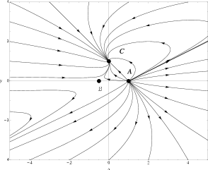
(a) Case $A<1$.

(b) Case $1<A<3$.

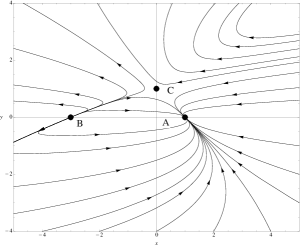
(c) Case $A>3$.

Figure 1: Phase plots of the system (19-21) for $\alpha<2$ and dust ($w=0$).

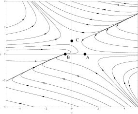
(a) Case $A<1$.

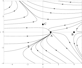
(b) Case $1<A<3$.

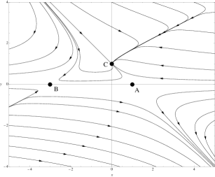
(c) Case $A>3$.

Figure 2: Phase plots of the system (19-21) for $\alpha>2$ and dust ($w=0$).

3.3 Asymptotic Analysis

Looking at (25) it appears clear that the phase plane is not compact and it is possible that the dynamical system (23-24) has a nontrivial asymptotic structure. Thus the above discussion would be incomplete without checking the existence of fixed points at infinity (i.e. when the variables $x$ or $y$ diverge) and calculating their stability. Such points represent regimes in which one or more of the terms in the Friedmann equation (17) become dominant and should not be confused with the time asymptotics i.e. $t\rightarrow\infty$.

The asymptotic analysis can be easily performed by compactifying the phase space using the so called Poincar$\acute{e}$ method [60]. The compactification can be achieved by transforming to polar coordinates $(r(\cal{N}),\theta(\cal{N}))$:

$$x\rightarrow r\cos\theta\;,\qquad\qquad y\rightarrow r\sin\theta\;,$$ (33)

and substituting $r\rightarrow\frac{{\cal R}}{1-{\cal R}}$ so that the regime $r\rightarrow\infty$ corresponds to ${\cal R}\rightarrow 1$. Using the coordinates (33) and taking the limit ${\cal R}\rightarrow 1$, the equations (23) can be written as

$$\mathcal{R}^{\prime} = \frac{1}{12}(A-3)(\alpha\sin 2\phi+\alpha\cos 2\phi-\alpha+4)(3w\cos\phi-2\sin\phi+\cos\phi),$$ (34)

$$\theta^{\prime} = -\frac{\alpha(A-3)}{4(\rho-1)}\,\left[\left(1+3\,w\right)\,\cos\theta-2\,\sin\theta\right]\,\left(-1+\cos 2\,\theta-\sin 2\,\theta\right).$$ (35)

It can be proven that the existence and the stability of the fixed points can be derived analyzing the fixed point of the equation for $\theta$ [60]. Setting $\theta^{\prime}=0$, we obtain six fixed points which are given in Table 3. The solution associated with the asymptotic fixed points can be derived in the same way of the ones for the finite case and are also shown in Table 3. For details on this derivation we refer the reader to the detailed discussion in [54]. The solutions associated to the asymptotic fixed points are of two basic types. A first one is an exponential growth i.e. a deSitter phase (points $\mathcal{A}$-$\mathcal{B}$) and a second one whose growth and decay depends on the values of $\alpha$ and $w$. In particular they can represent bounces or cosmologies in which the deceleration parameter changes sign.

Table 3: Asymptotic fixed points, $\theta$ coordinates and solutions for the system (19-21).

Point	$\theta$	Behavior
$\mathcal{A}_{\infty}$	0	$a=a_{0}\exp[\frac{1}{4}{C_{1}^{2}}\,(t-{t_{0}})]$
$\mathcal{B}_{\infty}$	$\pi$	$a=a_{0}\exp\left[\frac{1}{4}{C_{1}^{2}}\,(t-{t_{0}})\right]$
$\mathcal{C}_{\infty}$	$3\pi/4$	$a=a_{0}\exp\left[-\left(\frac{(\alpha-1)(t-t_{0})}{2-\alpha}\right)^{\frac{\alpha-2}{\alpha-1}}\right]$
$\mathcal{D}_{\infty}$	$7\pi/4$	$a=a_{0}\exp\left[-\left(\frac{(\alpha-1)(t-t_{0})}{2-\alpha}\right)^{\frac{\alpha-2}{\alpha-1}}\right]$
$\mathcal{E}_{\infty}$	$\arctan\left(\frac{1+3w}{2}\right)$	$a_{0}\exp\left[\left(t-t_{0}\right)^{r}\left(\frac{-3(2-\alpha)w(3w+2)-3\alpha+2}{3(\alpha-2)(w+1)(3w-1)}\right)^{r}\right]$
$\mathcal{F}_{\infty}$	$\arctan\left(\frac{1+3w}{2}\right)+\pi$	$a_{0}\exp\left[\left(t-t_{0}\right)^{r}\left(\frac{-3(2-\alpha)w(3w+2)-3\alpha+2}{3(\alpha-2)(w+1)(3w-1)}\right)^{r}\right]$
$r=1+\frac{4}{9(\alpha-2)w^{2}+6(\alpha-2)w-3\alpha+2}$

Table 4: Stability of the asymptotic fixed points for the system (19-21).

Point		$A<3$			$A>3$
	$\alpha<0$	$0<\alpha<2$	$\alpha>2$	$\alpha<0$	$0<\alpha<2$	$\alpha>2$
$\mathcal{A}_{\infty}$	attractor	saddle	saddle	repeller	saddle	saddle
$\mathcal{B}_{\infty}$	repeller	saddle	saddle	attractor	saddle	saddle
$\mathcal{C}_{\infty}$	saddle	repeller	saddle	saddle	attractor	saddle
$\mathcal{D}_{\infty}$	saddle	attractor	saddle	saddle	repeller	saddle

Finally, the stability of the asymptotic fixed points can be obtained with the standard methods of the dynamical system. The results for the first four fixed points ($\mathcal{A}_{\infty}$-$\mathcal{D}_{\infty}$) is given in Table 4.

The same is not true for the last two fixed points ($\mathcal{E}_{\infty}$, $\mathcal{F}_{\infty}$) whose stability do depend on $w$. The character of these points is complicated by the fact that the value of $\mathcal{R}^{\prime}$, whose sign is connected to the stability in the radial direction is zero. Fortunately this problem can be solved noting that the next to leading term in the full the equation for $\mathcal{R}^{\prime}$ is finite and different from zero and can give information on the behavior of the function $\mathcal{R}^{\prime}$ nearby $\mathcal{R}=1$. The stability thus obtained is shown in Tables 5 and 6.

Table 5: Stability of the asymptotic fixed point $\mathcal{E}_{\infty}$.

	attractor	repeller	saddle
	$\alpha\leq-10\land 3<A<\frac{3\alpha-6}{\alpha+10}$
$w=0$	$-10<\alpha<0\land A>3$	$-10<\alpha<0\land A<\frac{3\alpha-6}{\alpha+10}$	otherwise
	$\alpha>0\land\frac{3\alpha-6}{\alpha+10}<A<3$
$w=1/3$	$\alpha<0\land A>3$	$\alpha<0\land A<0$	otherwise
	$\alpha>0\land 0<A<3$
	$\alpha<0\land A>3$
$w=1$	$0<\alpha\leq 5\land\frac{3\alpha-6}{\alpha-5}<A<3$	$\begin{array}[]{c}\alpha<0\land A<\frac{3\alpha-6}{\alpha-5}\\ \alpha>5\land A>\frac{3\alpha-6}{\alpha-5}\end{array}$	otherwise
	$\alpha>5\land A<3$

Table 6: Stability of the asymptotic fixed point $\mathcal{F}_{\infty}$.

	attractor	repeller	saddle
$w=0$	$\alpha<-10\land A<3$	$\begin{array}[]{c}\alpha<-10\land A>\frac{3\alpha-6}{\alpha+10}\\ \alpha>0\land A<\frac{3\alpha-6}{\alpha+10}\\ \end{array}$	otherwise
	$-10<\alpha<0\land\frac{3\alpha-6}{\alpha+10}<A<3$
	$\alpha>0\land A>3$
$w=1/3$	$\alpha<0\land 0<A<3$	$\alpha<0\land A<0$	otherwise
	$\alpha>0\land A>3$
$w=1$	$\alpha<0\land\frac{3\alpha-6}{\alpha-5}<A<3$	$0<\alpha<5\land A<\frac{3\alpha-6}{\alpha-5}$	otherwise
	$0<\alpha\leq 5\land A>3$
	$\alpha>5\land 3<A<3\frac{3\alpha-6}{\alpha-5}$

Now that the asymptotic fixed points and their stability has been determined let us look in more detail to their physical interpretation.

As said before, these points are characterized by one or more variables to become infinite. In terms of the definitions (18), this corresponds to the fact that either the quantities in the numerators are infinite or the ones in the denominators approach zero. In the first case we are probably seeing some kind of singularity of the model. In the second we are seeing a change in sign of the expansion, which in turns corresponds to a maximum or a minimum of the scale factor. It is important to bear in mind that, because of our definition of the time variable, when an orbits “reaches” an infinite point the time coordinate changes sign and the Universe follows the orbit with a reversed orientation. In some sense one can picture this transition as the fact that the asymptotic points are the doorway to a mirror phase space in which the orbit orientation and stability of the fixed points are reversed.

In the pure GR framework, where the cosmological equation predict (almost) always a monotonic behavior of the scale factor, extrema of the scale factors can occur only at the origin of time. We usually talk then of “bounces” or “(re)collapsing universes” depending on the sing of the second derivative of the scale factor (or $\dot{H}$). In more complex cosmological models, like e.g. $f(R)$ gravity [61], the behavior is more complicated and the scale factor can have in principle a series of extrema located at a generic instant. This is the case also for the RG cosmologies. However, we will retain the traditional names to indicate such features of the scale factor.

Let us focus, for example, on the conditions to have a bounce i.e. a situation in which $\dot{a}=0$ and $\ddot{a}>0$ . In terms of the dynamical variables these can be translated in the requirement that one has an asymptotic attractor characterized by $H=0=\dot{a}$ and that this attractor lays in the part of the phase space for which $-(1+q)<0$ which is determined via (30). Using this condition it turns out, for example, that for $\alpha>0$ only $\mathcal{D}_{\infty}$ can represent a bounce. The results for the other points can be found in Table 7.

Table 7: Physical interpretation of the Asymptotic Attractors.

Point	Bounce	(Re)Collapsing	Singularity
$\mathcal{A}_{\infty}$	No	No	Yes
$\mathcal{B}_{\infty}$	No	No	Yes
$\mathcal{C}_{\infty}$	No	$0<\alpha<2$, $A>3$	Otherwise
$\mathcal{D}_{\infty}$	$0<\alpha<2$, $A>3$	No	Otherwise
$\mathcal{E}_{\infty}(w=0)$	$\alpha\leq-10\land 3<A<\frac{3\alpha-6}{\alpha+10}$	$0<\alpha<\frac{6+10A}{3-A}\land-\frac{3}{5}<A<0$	Otherwise
	$-10<\alpha<0\land A>3$	$0<A<3$, $0<\alpha<2$
$\mathcal{F}_{\infty}(w=0)$	$\alpha\leq-10\land 3<A<\frac{3\alpha-6}{\alpha+10}$	$0<\alpha<\frac{6+10A}{3-A}\land-\frac{3}{5}<A<0$	Otherwise
	$-10<\alpha<0\land A>3$	$0<A<3$, $0<\alpha<2$
$\mathcal{E}_{\infty}(w=1/3)$	$\alpha<0\land A>3$	$0<\alpha<2\land 0<A<3$	Otherwise
$\mathcal{F}_{\infty}(w=1/3)$	$\alpha<0\land A>3$	$0<\alpha<2\land 0<A<3$	Otherwise
$\mathcal{E}_{\infty}(w=1)$	$\alpha\leq-10\land 3<A<\frac{3\alpha-6}{\alpha+10}$	$0<\alpha<\frac{6+10A}{3-A}\land-\frac{3}{5}<A<0$	Otherwise
	$-10<\alpha<0\land A>3$	$0<A<3$, $0<\alpha<2$
$\mathcal{F}_{\infty}(w=1)$	$\alpha\leq-10\land 3<A<\frac{3\alpha-6}{\alpha+10}$	$0<\alpha<\frac{6+10A}{3-A}\land-\frac{3}{5}<A<0$	Otherwise
	$-10<\alpha<0\land A>3$	$0<A<3$, $0<\alpha<2$

Figure 3: Evolution of some key cosmological quantities in RG cosmologies with $w=0$ $A=1/2$, $\alpha=1$ (dashed) compared with the ones of GR$\Lambda$ (solid). We have chosen as initial condition the phase space point $(x=1.1,y=0.1)$ present in both the phase spaces. The index 0 is associated to the value of all the quantities in this point. Upper panel: Semi logarithmic plot of $H/H_{0}$ as function of $\ln(a/a_{0})$. Lower panel: Logarithmic plot of $\frac{8}{3}\pi G\rho$ as a function of $\ln(a/a_{0})$. The energy density is not plotted because its behavior is exactly matched in the two models.

Figure 4: Evolution of the term $\frac{BH^{\alpha}}{3-A}$ in RG cosmologies with $w=0$ $A=1/2$, $\alpha=1$, $B=2$ (dashed) compared with the $\Lambda$ term in GR (solid). We have chosen as initial condition the phase space point $(x=1.1,y=0.1)$ and the index 0 is associated to the value of all the quantities in this point.

4 Conclusions

In this paper we have investigated the effect on cosmological scale of a quantum gravity related decaying of the cosmological constant. This investigation was performed using the Dynamical System Approach that allows a semi-quantitative treatment of the model via the construction of a phase space directly connected to the behavior of the equations. The phase space is two dimensional and it contains a total of nine fixed point, of which three are finite and six are asymptotical. The stability of these points is found to depend on the parameters $A$ and $\alpha$, but not on $B$ which has a marginal position in the entire analysis. The determination of the fixed points and their stability allows us to infer the shape of the phase space orbits and to deduce the qualitative features of the cosmic histories possible in this models.

Among these, one is particularly relevant in terms of the problem of dark energy domination i.e. the presence of a cosmic history characterized by a first phase in which the scale factor grows as a power law with exponent included in $]0,1[$ followed by a second phase with a faster growth. In terms of the features of the phase space that such scenario can be realized if one has an unstable fixed point representing the first phase and an attractor representing the second. Looking at Tables 2 - 6 one can easily see that there is only is one set of the parameters $(A,\alpha)$ for which this can be realized: $(A<\frac{1+3w}{1+w},\;\alpha<2)$, for which $\mathcal{A}$ is a repeller. It is reassuring to notice that in this case $A$ is of the order unity and, as $A=\xi^{2}\lambda_{\ast}$, we deduce that also $\xi$ is of the order unity being $\lambda_{\ast}<1/2$.

When these conditions are satisfied there can exist, depending on initial conditions, one orbit that starts at $\mathcal{A}$ and either go directly to $\mathcal{C}$ or bounce at $\mathcal{E}_{\infty}$. The first case can be seen as a “classical” Friedmann-de Sitter transition. In the second case the cosmological evolution could be richer because the solution $\mathcal{E}_{\infty}$ can indicate, depending on the sign of $\alpha$, a growth whose rate saturates or an expansion phase comparable with a de Sitter one. One could interpret this as a ”two regimes“ dark energy phase. Note that, as we have seen, in the fixed points $\mathcal{A}$ and $\mathcal{B}$ the parameter $B$ is zero these points represent states for the cosmology that are indistinguishable from standard general relativity. This means that our model in the neighborhood of these points is indistinguishable from the standard cosmology. An example of the evolution of some key cosmological quantities compared with the standard de Sitter cosmology is given in Figure 3, and in Figure 4 we compare the additional RG term in (17) with the standard cosmological constant.

It is important to emphasize that the standard experimental value of Newton’s constant, $G_{\rm exp}$, does not coincide with the value $G(k=\xi H_{0})$ which is relevant for cosmology today. $G_{\rm exp}$ is measured (today) at $k_{\rm exp}\propto\ell^{-1}$ where the length $\ell\equiv\ell_{\rm sol}$ is a typical solar system length scale, say $10^{12}$ m. Thus, in terms of the running Newton constant, $G_{\rm exp}=G(k=\xi^{\prime}/\ell_{\rm sol})$, since $\ell_{\rm sol}\ll H_{0}$. It is only the cosmological quantity $G(k=\xi H)$ which dynamically evolves in the fixed point regime, not $G_{\rm exp}$. This remark entails that the dynamical evolution of the cosmological Newton constant in the recent past does not ruin the predictions about primordial nucleosynthesis which requires that $G(k=\xi H_{\rm nucl})$ coincides with $G_{\rm exp}$ rather precisely. In fact, at the time $t=t_{\rm nucl}$ of nucleosynthesis for which $H=H(t=t_{\rm nucl})$, the cosmological Newton constant was indeed $G(k=\xi H_{\rm nucl})\approx G_{\rm exp}$ since $ct_{\rm nucl}\approx H_{\rm nucl}^{-1}$ and $\ell_{\rm sol}$ are of the same order of magnitude.

The phase space structure also sheds light on aspects of the type of RG cosmologies not directly related to the problem of dark energy. For example, it is clear that it is possible to interpret the transition to a dark era as the beginning of a primordial inflationary phase. Our results then imply that there is only one set of values that allows a “graceful exit” i.e. the transition from inflation to a Friedmann cosmology. Specifically in the case $(A<\frac{1+3w}{1+w},\;\alpha>2)$ we can have this kind of scenario. However, since there is only one point which represents accelerating expansion one can see that the RG model can be used to represent either the inflationary era or the dark energy era, but not both.

Finally the analysis of the asymptotic fixed points gives information on the possibility of changes in the sign of expansion rates in this type of cosmologies. In general relativity such phases are normally associated either to the so-called ”bounces” and are associated to cyclic Universes (when $\dot{H}>0$) or to recollapsing universes (when $\dot{H}<0$). In modified theories of gravity changes in the sign of $H$ can occur also when the size of the Universe is large because the scale factor does not need to be monotonic [61]. In terms of the phase space this kind of behavior is associated to the presence of asymptotic attractors and the sign of the quantity $-(1+q)$ as expressed in (29) in the fixed point. In particular we have that if $-(1+q)>0$ we have a deceleration followed by an acceleration and if $-(1+q)<0$ the opposite situation. A quick analysis shows, for example, that only some of the asymptotic attractors for very specific values of the parameters can give origin to a bounce.

The previous results point towards a cosmology with interesting features that, in our opinion, deserves some more study. In particular one could try to test the transition to Dark Age we have found against the SnIa data to obtain some more constraints on the free parameters. This, and other issues, will be discussed in a following work.

References

- [1] M. Reuter. Nonperturbative evolution equation for quantum gravity. Phys. Rev. D, 57:971–985, 1998.
- [2] D. Dou and R. Percacci. The running gravitational couplings. Classical and Quantum Gravity, 15:3449–3468, November 1998.
- [3] W. Souma. Non-Trivial Ultraviolet Fixed Point in Quantum Gravity. Progress of Theoretical Physics, 102:181–195, July 1999.
- [4] O. Lauscher and M. Reuter. Ultraviolet fixed point and generalized flow equation of quantum gravity. Phys. Rev. D, 65(2):025013–+, January 2002.
- [5] O. Lauscher and M. Reuter. Flow equation of quantum Einstein gravity in a higher-derivative truncation. Phys. Rev. D, 66(2):025026–+, July 2002.
- [6] O. Lauscher and M. Reuter. Is quantum Einstein gravity nonperturbatively renormalizable? Classical and Quantum Gravity, 19:483–492, February 2002.
- [7] M. Reuter and F. Saueressig. Renormalization group flow of quantum gravity in the Einstein-Hilbert truncation. Phys. Rev. D, 65(6):065016–+, March 2002.
- [8] M. Reuter and F. Saueressig. A class of nonlocal truncations in quantum Einstein gravity and its renormalization group behavior. Phys. Rev. D, 66(12):125001–+, December 2002.
- [9] D. F. Litim. Fixed Points of Quantum Gravity. Physical Review Letters, 92(20):201301–+, May 2004.
- [10] A. Bonanno and M. Reuter. Proper time flow equation for gravity. Journal of High Energy Physics, 2:35–+, February 2005.
- [11] A. Codello and R. Percacci. Fixed Points of Higher-Derivative Gravity. Physical Review Letters, 97(22):221301–+, December 2006.
- [12] M. Reuter and H. Weyer. The role of background independence for asymptotic safety in Quantum Einstein Gravity. General Relativity and Gravitation, 41:983–1011, April 2009.
- [13] M. Reuter and H. Weyer. Background independence and asymptotic safety in conformally reduced gravity. Phys. Rev. D, 79(10):105005–+, May 2009.
- [14] P. F. Machado and R. Percacci. Conformally reduced quantum gravity revisited. Phys.Rev.D, 80:024020, April 2009.
- [15] E. Manrique and M. Reuter. Bare vs. Effective Fixed Point Action in Asymptotic Safety: The Reconstruction Problem. PoS CLAQG08, page 001, 2009.
- [16] S. Weinberg. Ultraviolet divergences in quantum theories of gravitation. In S.W. Hawking and W. Israel, editors, General Relativity, an Einstein Centenary Survey. Cambridge University Press, 1979.
- [17] A. M. Polyakov. A Few Projects in String Theory. PUPT-1394, April 1993.
- [18] R. Percacci and D. Perini. Constraints on matter from asymptotic safety. Phys. Rev. D, 67(8):081503, April 2003.
- [19] Max Niedermaier and Martin Reuter. The asymptotic safety scenario in quantum gravity. Living Reviews in Relativity, 9:5, December 2006.
- [20] D. Benedetti, P. F. Machado, and F. Saueressig. Four-derivative Interactions in Asymptotically Safe Gravity. In J. Kowalski-Glikman, R. Durka, & M. Szczachor, editor, American Institute of Physics Conference Series, volume 1196 of American Institute of Physics Conference Series, pages 44–51, December 2009.
- [21] D. Benedetti, P. F. Machado, and F. Saueressig. Taming perturbative divergences in asymptotically safe gravity. Nuclear Physics B, 824:168–191, January 2010.
- [22] A. Codello, R. Percacci, and C. Rahmede. Investigating the ultraviolet properties of gravity with a Wilsonian renormalization group equation. Annals of Physics, 324:414–469, February 2009.
- [23] A. Codello, R. Percacci, and C. Rahmede. Ultraviolet Properties of f(R)-GRAVITY. International Journal of Modern Physics A, 23:143–150, 2008.
- [24] A. Bonanno. Astrophysical implications of the Asymptotic Safety Scenario in Quantum Gravity. ArXiv e-prints, November 2009.
- [25] A. Bonanno and M. Reuter. Quantum gravity effects near the null black hole singularity. Phys. Rev. D, 60(8):084011–+, October 1999.
- [26] A. Bonanno and M. Reuter. Renormalization group improved black hole spacetimes. Phys. Rev. D, 62(4):043008–+, August 2000.
- [27] A. Bonanno and M. Reuter. Spacetime structure of an evaporating black hole in quantum gravity. Phys. Rev. D, 73(8):083005–+, April 2006.
- [28] A. Bonanno and M. Reuter. Cosmology of the Planck era from a renormalization group for quantum gravity. Phys. Rev. D, 65(4):043508–+, February 2002.
- [29] A. Bonanno, G. Esposito, and C. Rubano. A Class of Renormalization Group Invariant Scalar Field Cosmologies. General Relativity and Gravitation, 35:1899–1907, November 2003.
- [30] A. Bonanno, G. Esposito, and C. Rubano. Arnowitt Deser Misner gravity with variable G and and fixed-point cosmologies from the renormalization group. Classical and Quantum Gravity, 21:5005–5016, November 2004.
- [31] A. Bonanno, G. Esposito, and C. Rubano. Improved Action Functionals in Non-Perturbative Quantum Gravity. International Journal of Modern Physics A, 20:2358–2363, 2005.
- [32] A. Bonanno, G. Esposito, C. Rubano, and P. Scudellaro. The accelerated expansion of the universe as a crossover phenomenon. Classical and Quantum Gravity, 23:3103–3110, May 2006.
- [33] A. Bonanno and M. Reuter. A cosmology of the Planck era from the renormalization group for quantum gravity. In I. Ciufolini, E. Coccia, M. Colpi, V. Gorini, and R. Peron, editors, Recent Developments in Gravitational Physics, pages 461–+, 2006.
- [34] M. Reuter and H. Weyer. Quantum gravity at astrophysical distances? Journal of Cosmology and Astro-Particle Physics, 12:1–+, December 2004.
- [35] J. Alexandre, V. Branchina, and J. Polonyi. Instability induced renormalization. Physics Letters B, 445:351–356, January 1999.
- [36] O. Lauscher, M. Reuter, and C. Wetterich. Rotation symmetry breaking condensate in a scalar theory. Phys. Rev. D, 62(12):125021–+, December 2000.
- [37] A. Bonanno and G. Lacagnina. Spontaneous symmetry breaking and proper-time flow equations. Nuclear Physics B, 693:36–50, August 2004.
- [38] J. A. S. Lima. Thermodynamics of decaying vacuum cosmologies. Phys. Rev. D, 54:2571–2577, August 1996.
- [39] A. Bonanno and M. Reuter. Cosmology with self-adjusting vacuum energy density from a renormalization group fixed point. Physics Letters B, 527:9–17, February 2002.
- [40] A. Bonanno and M. Reuter. Cosmological Perturbations in Renormalization Group Derived Cosmologies. International Journal of Modern Physics D, 13:107–121, 2004.
- [41] E. Bentivegna, A. Bonanno, and M. Reuter. Confronting the IR fixed point cosmology with high-redshift observations. Journal of Cosmology and Astro-Particle Physics, 1:1–+, January 2004.
- [42] M. Reuter and F. Saueressig. Nonlocal quantum gravity and the size of the universe. Fortschritte der Physik, 52:650–654, June 2004.
- [43] M. Reuter and H. Weyer. Renormalization group improved gravitational actions: A Brans-Dicke approach. Phys. Rev. D, 69(10):104022–+, May 2004.
- [44] M. Reuter and H. Weyer. Running Newton constant, improved gravitational actions, and galaxy rotation curves. Phys. Rev. D, 70(12):124028–+, December 2004.
- [45] G. Esposito, C. Rubano, and P. Scudellaro. Spherically symmetric ADM gravity with variable G and . Classical and Quantum Gravity, 24:6255–6266, December 2007.
- [46] M. Reuter and F. Saueressig. From big bang to asymptotic de Sitter: complete cosmologies in a quantum gravity framework. Journal of Cosmology and Astro-Particle Physics, 9:12–+, September 2005.
- [47] A. Bonanno and M. Reuter. Entropy signature of the running cosmological constant. Journal of Cosmology and Astro-Particle Physics, 8:24–+, August 2007.
- [48] A. Bonanno and M. Reuter. Primordial entropy production and -driven inflation from Quantum Einstein Gravity. Journal of Physics Conference Series, 140(1):012008–+, November 2008.
- [49] O. I. Bogoyavlensky. Methods in the qualitative theory of dynamical systems in astrophysics and gas dynamics. Springer Series in Soviet Mathematics, Berlin: Springer, 1985, 1985.
- [50] G F R Ellis J Wainwright, editor. Dynamical Systems in Cosmology. Cambridge University Press, 1997.
- [51] Edmund J. Copeland, Shuntaro Mizuno, and Maryam Shaeri. Dynamics of a scalar field in Robertson-Walker spacetimes. Phys. Rev., D79:103515, 2009.
- [52] Edmund J. Copeland, Andrew R Liddle, and David Wands. Exponential potentials and cosmological scaling solutions. Phys. Rev., D57:4686–4690, 1998.
- [53] S. Carloni, S. Capozziello, J. A. Leach, and P. K. S. Dunsby. Cosmological dynamics of scalar-tensor gravity. Class. Quant. Grav., 25:035008, 2008.
- [54] Sante Carloni, Peter K. S. Dunsby, Salvatore Capozziello, and Antonio Troisi. Cosmological dynamics of gravity. Class. Quant. Grav., 22:4839–4868, 2005.
- [55] Jannie A. Leach, Sante Carloni, and Peter K. S. Dunsby. Shear dynamics in Bianchi I cosmologies with -gravity. Class. Quant. Grav., 23:4915–4937, 2006.
- [56] M. Abdelwahab, S Carloni, and P K. S. Dunsby. Cosmological dynamics of exponential gravity. Class. Quant. Grav., 25:135002, 2008.
- [57] S. Carloni, A. Troisi, and P. K. S. Dunsby. Some remarks on the dynamical systems approach to fourth order gravity. Gen. Rel. Grav., 41:1757–1776, 2009.
- [58] Sante Carloni, Emilio Elizalde, and Pedro J. Silva. An analysis of the phase space of Horava-Lifshitz cosmologies. Class. Quant. Grav., 27:045004, 2010.
- [59] Elisa Manrique, Martin Reuter, and Frank Saueressig. Bimetric renormalization group flows in quantum einstein gravity. eprint arXiv, 1006:99, Jun 2010. 35 pages, 3 figures.
- [60] S Lefschetz. Differential Equations: Geometric Theory. Dover (New York), 1977.
- [61] Sante Carloni, Peter K.S. Dunsby, and Deon M. Solomons. Bounce conditions in f(R) cosmologies. Class.Quant.Grav., 23:1913–1922, 2006.