Combinatorics of locally optimal RNA secondary structures

Abstract.

It is a classical result of Stein and Waterman that the asymptotic number of RNA secondary structures is $1.104366\cdot n^{-3/2}\cdot 2.618034^{n}$. Motivated by the kinetics of RNA secondary structure formation, we are interested in determining the asymptotic number of secondary structures that are locally optimal, with respect to a particular energy model. In the Nussinov energy model, where each base pair contributes $-1$ towards the energy of the structure, locally optimal structures are exactly the saturated structures, for which we have previously shown that asymptotically, there are $1.07427\cdot n^{-3/2}\cdot 2.35467^{n}$ many saturated structures for a sequence of length $n$. In this paper, we consider the base stacking energy model, a mild variant of the Nussinov model, where each stacked base pair contributes $-1$ toward the energy of the structure. Locally optimal structures with respect to the base stacking energy model are exactly those secondary structures, whose stems cannot be extended. Such structures were first considered by Evers and Giegerich, who described a dynamic programming algorithm to enumerate all locally optimal structures. In this paper, we apply methods from enumerative combinatorics to compute the asymptotic number of such structures. Additionally, we consider analogous combinatorial problems for secondary structures with annotated single-stranded, stacking nucleotides (dangles).

1. Introduction

Historically, the development of combinatorics for RNA secondary structures [35, 39] has been intimately related to the development of algorithms for RNA minimum free energy (MFE) secondary structure [45, 43, 15]. In particular, counting the number of secondary structures for sequence of length $n$ is essentially equivalent to computing the Boltzmann partition function, defined by $Z=\sum_{S}\exp(-E(S)/RT)$, where the sum is taken over all secondary structures $S$, the energy of $S$ is denoted by $E(S)$, $R\approx 1.959$ cal/mol is the universal gas constant, and $T$ absolute temperature.

Complex analysis is used to obtain the asymptotic enumeration results described in this article and related articles mentioned in the introduction. In particular, given a complex generating function $f(z)=\sum a_{n}z^{n}$, it is well-known from introductory complex analysis that $f$ converges in a circular region about the point of expansion out to the dominant, or nearest, singularity $r$, and thus the asymptotic order of magnitude of $a_{n}$ is approximately $r^{-n}$. Darboux’s theorem [29, 14] states that if $f(z)=\sum_{n=0}^{\infty}(r-z)^{\alpha}L(z)$, where $r>0$, $\alpha$ is not a positive integer, and $L$ is analytic in a disk of radius greater than $r$, then $\alpha_{n}\sim r^{\alpha-n}n^{\alpha-1}\frac{L(r)}{\Gamma(-\alpha)}$. This result was generalized by Bender [1], corrected by Meir and Moon [27], and further extended by Flajolet and Odlyzko [10] and by Drmota, Lalley and Woods (each of the latter worked independently) – see the exposition in [11] for discussion and references.

In [35], Stein and Waterman proved that the asymptotic number of secondary structures is $1.104366\cdot n^{-3/2}\cdot 2.618034^{n}$. Since that time, a number of additional results on the combinatorics of RNA structures have been obtained. In [18], Hofacker et al. derived a number of asymptotic results on the number of structures, expected number of base pairs, etc. for RNA secondary structures. Observing a correspondence with involutions, Haslinger and Stadler [13] provided an upper bound on the number of bi-secondary structures, i.e. structures having non-nested pseudoknots that can be presented as a union $S=S_{1}\cup S_{2}$ of disjoint secondary structures, and Rodland [30] studied the asymptotic number of a number of classes of pseudoknotted structures. Building on a remarkable and pioneering paper of Harer and Zagier [12], Vernizzi et al. [37] classified pseudoknotted RNA structures according to topological genus $g$, and then applied the work of Harer and Zagier to obtain recurrence relations for the number of pseudoknotted structures of genus $g$. In [31], Saule et al. provided a summary table of the asymptotic number of pseudoknotted structures structures, with respect to various allowed pseudoknots, and established the asymptotic number of pseudoknotted structures, with no restriction. In [20], Li and Reidys determined the asymptotic number of hybridizations of two interacting RNA structures. Moving away from counting the number of structures, Yoffe et al. [41] and Clote et al. [4] determined the asymptotic expected distance between the $5^{\prime}$ and $3^{\prime}$ ends of RNA sequence, where the $5^{\prime}$ to $3^{\prime}$ distance of a given structure $S$ on sequence $s_{1},\ldots,s_{n}$ is defined as the minimum number of backbone or base-pairing edges in a minimum length path from $s_{1}$ to $s_{n}$.

In [3], Clote computed the asymptotic number $1.07427\cdot n^{-3/2}\cdot 2.35467^{n}$ of saturated structures, defined by Zuker [42] as those for which no base pair can be added without violating the definition of secondary structure. In [5], Clote et al. provided another proof for the asymptotic number of saturated structures, which additionally yielded the asymptotic expected number of base pairs $0.337361\cdot n$ for saturated structures. An overview of methods for RNA enumerative combinatorics is given in Lorenz et al. [21], where additionally it is shown that the asymptotic number of shapes of secondary structures for a length $n$ sequence is $2.44251\cdot n^{-3/2}\cdot 1.32218^{n}$. In [18] Hofacker et al. showed that the asymptotic number of canonical secondary structures (those having no isolated base pair) is $2.1614\cdot n^{-3/2}\cdot 1.96798^{n}$, a result that was confirmed by a different method in Clote et al. [5], where additionally the expected number of base pairs was shown to be $0.31724\cdot n$.

A locally optimal, or kinetically trapped, secondary structure $S$ is one for which no secondary structure $T$, obtained from $S$ by the removal or addition of a single base pair, has lower energy. It follows that saturated structures are exactly the kinetically trapped structures with respect to the Nussinov energy model [28], in which each base pair receives a stabilizing energy contribution of $-1$. In this paper, we consider the base stacking energy model, in which each stacked base pair receives a stabilizing energy contribution of $-1$. Here, the base pair $(i,j)$ in secondary structure $S$ is defined to be a stacked base pair, provided that $(i-1,j+1)$ is also a base pair in $S$ – i.e. provided that there is an outer base pair that provides a stabilizing stacking energy. In [9], Evers and Giegerich describe a dynamic programming algorithm to enumerate all structures that are locally optimal with respect to the base stacking energy model; i.e. those structures in which no stem can be extended. The authors called such structures “saturated”. When a strictly positive minimal value is specified for the length of every stem, a structure is saturated in the sense of Zuker [42] if and only if it is saturated in the sense of Evers and Giegerich [9]. However, as mentioned in [3], when the lengths of stems are not constrained, there are structures that are saturated in the sense of Evers and Giegerich [9], but which are not saturated in the sense of Zuker [42]. For clarity of exposition, we will call a secondary structure G-saturated if no stem can be extended. In this paper, we give an enumerative framework based on weighted plane trees that allows us to enumerate G-saturated structures (as well as recover the enumeration of secondary structures and of saturated structures). We also consider analogous problems for structures with annotated single-stranded, stacked nucleotides (also called dangles).

Outline of paper

The plan of this paper is as follows. In Section 2, we define the notions of secondary structure and context free grammar, and provide context free grammars for various classes of secondary structures considered in the paper. In that section, we show that the asymptotic number of secondary structures with annotated dangles, as computed in the partition function of the Markham-Zuker software UNAFOLD [23], is $0.63998\cdot n^{-3/2}\cdot 3.06039^{n}$, exponentially larger than the number of all secondary structures $1.104366\cdot n^{-3/2}\cdot 2.618034^{n}$, previously established by Stein and Waterman [35]. This new result provides a partial explanation for M. Zuker’s observation (personal communication) that UNAFOLD requires substantially more computation time when dangles are included. In Section 3, we describe the computation of secondary structure melting curves with respect to the Nussinov energy model and the base stacking energy model. Figure 2 shows that folding is more cooperative in the base stacking energy model. In Section 4, we describe the correspondence between RNA secondary structures and plane trees, and then give generating functions for the number of secondary structures and locally optimal secondary structures, with respect to the Nussinov model and the base stacking energy model. In Section 5, we give asymptotic results on the number of secondary structures and locally optimal secondary structures, as well as their expected number of base pairs. In Section 6, we give similar asymptotic results when annotations for external dangles are included for each type of structure. Finally Section 7 summarizes our main contributions.

2. Definitions

Definition 1 (Secondary structure).

An RNA secondary structure for a given RNA sequence $a_{1},\ldots,a_{n}$ of length $n$ is defined to be a set $S$ of ordered pairs $(i,j)$, with $1\leq i<j\leq n$, such that the following conditions are satisfied.

1. Watson-Crick and wobble pairs: If $(i,j)\in S$, then $\{a_{i},a_{j}\}\in\{\{A,U\}\{G,C\}\{G,U\}\}$.

2. No base triples: If $(i,j)$ and $(i,k)$ belong to $S$, then $j=k$; if $(i,j)$ and $(k,j)$ belong to $S$, then $i=k$.

3. Nonexistence of pseudoknots: If $(i,j)$ and $(k,\ell)$ belong to $S$, then it is not the case that $i<k<j<\ell$.

4. Threshold requirement for hairpins: If $(i,j)$ belongs to $S$, then $j-i>\theta$, for a fixed value $\theta\geq 0$; i.e. there must be at least $\theta$ unpaired bases in a hairpin loop.

For software, such as mfold [43] and RNAfold [16], to predict RNA secondary structure, $\theta$ is taken to be $3$; i.e., for reasons related to steric constraints, every hairpin is required to contain at least three unpaired bases.

A base pair $(i,j)\in S$ is called a link. An element $i$ is said to be linked if it is involved in a link and free otherwise. A link $(i,j)$ is said to be stacked onto another link $(i^{\prime},j^{\prime})$ if $i^{\prime}=i+1$ and $j^{\prime}=j-1$. A stem is a maximal sequence $\ell_{0},\ldots,\ell_{k}$ of links such that $\ell_{i}$ is stacked onto $\ell_{i+1}$ for $0\leq i\leq k-1$; the value $k$ is called the length of the stem. In some applications a threshold condition on stems is required:

5. Threshold requirement for stems: Each stem has length at least $\tau$, for a fixed value $\tau\geq 0$.

Note that Condition (5) is of no effect for $\tau=0$.

In this paper, we are concerned with the asymptotic number of locally optimal structures. In order to employ generating functions, we will need to assume the homopolymer model (following a convention established by Stein and Waterman [35]), meaning that any position can pair with any other position (arbitrary base pairs, not only Watson-Crick and wobble pairs). We thus define a secondary structure of a homopolymer of length $n$ to be a set $S$ of base pairs $(i,j)$, where $1\leq i<j\leq n$, such that the previous conditions (2,3,4,5) are satisfied.

The following notion of context free grammar is used for two reasons: (1) to provide a clean and succinct definition for RNA secondary structure, with respect to a particular energy model, and (2) for certain enumeration results. See Lorenz et al. [21] for more on context free grammars and their application to combinatorics. In particular, we refer the reader to [21] for an explanation of the DSV method used in this article, which allows us to go directly from a context free grammar to a functional equation for generating functions.

Definition 2 (Context free grammar).

A context free grammar is given by $G=(V,\Sigma,R,S)$, where $V$ is a finite set of nonterminal symbols (also called variables), $\Sigma$ is a disjoint finite set of terminal symbols, $S\in V$ is the start nonterminal, and

$$R\subset V\times(V\cup\Sigma)^{*}$$

is a finite set of production rules. Elements of $R$ are usually denoted by $A\rightarrow w$, rather than $(A,w)$.

If $x,y\in(V\cup\Sigma)^{*}$ and $A\rightarrow w$ is a rule, then by replacing the occurrence of $A$ in $xAy$ we obtain $xwy$. Such a derivation in one step is denoted by $xAy\Rightarrow_{G}xwy$, while the reflexive, transitive closure of $\Rightarrow_{G}$ is denoted $\Rightarrow^{*}_{G}$. The language generated by context free grammar $G$ is denoted by $L(G)$, and defined by

$$L(G)=\{w\in\Sigma^{*}:S\Rightarrow^{*}_{G}w\}.$$

Now, in the following sections, we give context free grammars for RNA secondary structures, including structures with explicitly annotated dangles. Using the correspondence between grammar and recursions for dynamic programming, each grammar corresponds to an algorithm for the partition function for secondary structures with respect to a different energy model – the Nussinov model, the base stacking energy model, the Turner model, the Turner model with a rigorous treatment of dangles, the Turner model with external dangles. For notational simplicity, we take $\theta$, the minimum number of unpaired bases in a hairpin loop to be $1$ (see condition 4 of Definition 1). It is not difficult to extend the grammar for any fixed value of $\theta$.

Nussinov energy model

In [28], Nussinov and Jacobson describe a dynamic programming algorithm to compute the minimum energy structure for a simple energy model, in which each base pair constitutes an energy term of $-1$.

It is well-known [21] that the following unambiguous grammar $G_{1}$ generates all secondary structures of the homopolymer model with $\theta=1$. Here $G_{1}$ has start non-terminal symbol $S$, and terminal symbols $\bullet,\,\mbox{\bf{(}}\,,\,\mbox{\bf{)}}\,$. The non-terminal symbol $S$ generates all non-empty secondary structures by using the following grammar (or production) rules.

$$S \rightarrow \bullet|\,\mbox{\bf{(}}\,S\,\mbox{\bf{)}}\,|S\,\mbox{\bf{(}}\,S\,\mbox{\bf{)}}\,$$

Let $S(z)$ denote the complex generating function $S(z)=\sum_{n=0}^{\infty}s_{n}z^{n}$, where Taylor coefficient $[z^{n}]S(z)$ is the number $s_{n}$ of secondary structures for a homopolymer of size $n$. By the DSV methodology [5, 21], we have

$$S(z)=S=z+zS+z^{2}S+z^{2}S^{2}.$$

Introducing the auxilliary variable $u$ to count number of base pairs, we have

(1) $$S(z,u)=S=z+zS+uz^{2}S+uz^{2}S^{2}=\displaystyle\sum_{n}\sum_{k\leq n}s_{k,n}u^{k}z^{n}$$

where $s_{k,n}$ denotes the number of secondary structures on a length $n$ homopolymer, having exactly $k$ base pairs. It follows that

$$\frac{\partial S(z,u)}{\partial u} = \sum_{n}\sum_{k\leq n}ks_{k,n}u^{k-1}z^{n}$$

hence

(2) $$[z^{n}]\frac{\partial S(z,u)}{\partial u}(z,1)=\sum_{k\leq n}ks_{k,n}.$$

Since

$$[z^{n}]S(z,1)=\sum_{k\leq n}s_{k,n}$$

is the number of secondary structures on a homopolymer of length $n$, it follows that the asymptotic expected energy over all secondary structures of a homopolymer of length $n$, with respect to the Nussinov energy model, is equal to $-1$ times the asymptotic expected number of base pairs

(3) $$-\lim_{n\rightarrow\infty}\frac{[z^{n}]\frac{\partial S(z,u)}{\partial u}(z,1)}{[z^{n}]S(z,1)}.$$

Base stacking energy model

In the base stacking energy model, an energy term of $-1$ is assigned to each base pair $(i,j)$ of structure $S$, provided that $(i,j)$ has an outer stacking pair – i.e. provided that $(i+1,j-1)\in S$. The set of all secondary structures is generated by the context free grammar $G_{2}$ with non-terminals $S,T$, start symbol $S$, and terminals $\bullet,\,\mbox{\bf{(}}\,,\,\mbox{\bf{)}}\,$ with the following rules:

$$S \rightarrow \bullet|S\bullet|T|ST$$

$$T \rightarrow \,\mbox{\bf{(}}\,\bullet\,\mbox{\bf{)}}\,|\,\mbox{\bf{(}}\,S\bullet\,\mbox{\bf{)}}\,|\,\mbox{\bf{(}}\,T\,\mbox{\bf{)}}\,|\,\mbox{\bf{(}}\,ST\,\mbox{\bf{)}}\,$$

Here, the non-terminal $S$ generates all secondary structures, while the non-terminal $T$ generates all secondary structures, such that the first and last positions are base-paired together. By introducing auxilliary non-terminal $T$, we can count the number of stacked base pairs, as well as the number of base pairs. It is not difficult to show by induction that $G_{2}$ is an unambiguous grammar that generates all secondary structures, hence is equivalent to the previous grammar $G_{1}$.

By the DSV methodology [5, 21], the generating function $S(z)=\sum_{n}s_{n}z^{n}$ satifies the following equations

$$S(z)=S = z+zS+T+ST$$

$$T(z)=T = z^{2}T+z^{2}ST+z^{3}+z^{3}S.$$

Introducing the auxilliary variables $u,v$ responsible for counting the number of base pairs resp. number of stacked base pairs, we have

(4) $$S(z,u,v)=S = z+zS+T+ST$$

$$T(z,u,v)=T = uvz^{2}T+uz^{2}ST+uz^{3}+uz^{3}S.$$

Letting $s_{k,m,n}$ denote the number of secondary structures on a length $n$ homopolymer, having $k$ stacked base pairs and $m$ base pairs, we have

$$S(z,u,v) = \sum_{n}\sum_{k,m\leq n}s_{k,m,n}u^{k}v^{m}z^{n}$$

$$\frac{\partial}{\partial u}S(z,u,v) = \sum_{n}\sum_{k,m\leq n}ks_{k,m,n}u^{k-1}v^{m}z^{n}$$

hence

(5) $$[z^{n}]\frac{\partial S(z,u,v)}{\partial u}(z,1,1) = \sum_{k,m\leq n}ks_{k,m,n}.$$

Since $S(z,1,1)$ is is the number of secondary structures on a homopolymer of length $n$, it follows that the asymptotic expected energy over all secondary structures of a homopolymer of length $n$, with respect to the base stacking energy model, is equal to $-1$ times the asymptotic expected number of stacked base pairs,

(6) $$-\lim_{n\rightarrow\infty}\frac{\frac{\partial S(z,u,v)}{\partial u}(z,1,1)}{[z^{n}]S(z,1,1)}.$$

Grammar for McCaskill algorithm

All thermodynamics-based RNA secondary structure prediction algorithms use the Turner nearest neighbor energy model [25, 40], which contains free energy parameters for base stacking, single nucleotide dangles, hairpins, bulges, internal loops and multiloops. These parameters are obtained by a least squares fit of UV absorption data in optical melting experiments. For instance, at $37^{\circ}$ C the RNA-RNA stacking free energy of $\begin{array}[]{ll}\mbox{$5^{\prime}$-{\tt AC}-$3^{\prime}$}\\ \mbox{$3^{\prime}$-{\tt UG}-$5^{\prime}$}\\ \end{array}$ is $-2.24$ kcal/mol and that of $\begin{array}[]{ll}\mbox{$5^{\prime}$-{\tt CC}-$3^{\prime}$}\\ \mbox{$3^{\prime}$-{\tt GG}-$5^{\prime}$}\\ \end{array}$ is $-3.36$ kcal/mol [40]. Software such as mfold of Zuker [46] and RNAfold from Vienna RNA Package [17] use the Turner energy model, while alternative approaches, such as Pfold [19] use stochastic context free grammars.

In [26], McCaskill describes a cubic time, dynamic programming algorithm to compute the partition function $Z=\sum_{S}\exp(-E(S)/RT)$ over all secondary structures $S$ of a given RNA sequence. Here $R$ is the universal gas constant, $T$ is absolute temperature, and $E(S)$ is the energy of structure $S$ with respect to the Turner energy model [40]. By analyzing McCaskill’s recursions, we obtain the following grammar $G_{3}$, which generates the same set of secondary structures as that generated by $G_{1},G_{2}$; however, by permitting the classification of various types of loops, the grammar $G_{3}$ will permit us later to incorporate energy terms for dangles, also known as single-stranded, stacked nucleotides, into our considerations. A stacked base pair in secondary structure $S$ is given by base pair $(i,j)\in S$, such that $(i-1,j+1)\in S$. A hairpin loop in secondary structure $S$ is given by base pair $(i,j)\in S$, such that $i+1,\ldots,j-1$ are unpaired in $S$. A left bulge of $S$ is given by base pairs $(i,j),(k,\ell)\in S$, such that $i+1<k<\ell<j$ and $\ell+1=j$. A right bulge of $S$ is given by base pairs $(i,j),(k,\ell)\in S$, such that $i<k<\ell<j-1$ and $i+1=k$. An internal loop of $S$ is given by base pairs $(i,j),(k,\ell)\in S$, such that $i+1<k<\ell<j-1$; i.e. an internal loop is comprised of both a left and right bulge. A multiloop $M$ of $S$ is given by base pairs $(i,j),(k_{1},\ell_{1}),\ldots,(k_{r},\ell_{r})\in S$, such that $i<k_{1}<\ell_{1}<\cdots<k_{r}<\ell_{r}<j$, where $r\geq 2$, and positions $i+1,\ldots,k_{1}-1,\ell_{1}+1,\ldots,k_{2}-1,\ell_{2}+1,\ldots,k_{r}-1,\ell_{r}+1,\ldots,j-1$ are all unpaired in $S$. For any positions $i<x<y<j$, where we do not require $x$ or $y$ to be base-paired, we say that the multiloop restricted to $[x,y]$ has $c$ components, if exactly $c$ of the base pairs $(k_{1},\ell_{1}),\ldots,(k_{r},\ell_{r})$ are found in the interval $[x,y]$. See Figure 1 for an illustration of various loops, and see [45, 44] for more on loop classification and the Turner energy model.

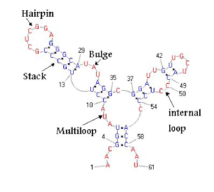
Figure 1. Secondary structure together with various loops: stacked base pair, hairpin, bulge, internal loop, multiloop.

Let grammar $G_{3}$ contain non-terminal symbols $S$ (start), $U$ (unpaired portion), $B$ (base-paired portion), $M_{1}$ (multiloop with exactly one component), $M$ (multiloop with at least one component), with the following production rules

$$S \rightarrow \bullet|B|S\bullet|SB$$

$$B \rightarrow \,\mbox{\bf{(}}\,U\,\mbox{\bf{)}}\,|\,\mbox{\bf{(}}\,B\,\mbox{\bf{)}}\,|\,\mbox{\bf{(}}\,UB\,\mbox{\bf{)}}\,|\,\mbox{\bf{(}}\,BU\,\mbox{\bf{)}}\,|\,\mbox{\bf{(}}\,UBU\,\mbox{\bf{)}}\,|\,\mbox{\bf{(}}\,MM_{1}\,\mbox{\bf{)}}\,$$

$$U \rightarrow \bullet|\bullet U$$

$$M_{1} \rightarrow B|BU$$

$$M \rightarrow M_{1}|UM_{1}|MM_{1}$$

It is not difficult to show that $G_{3}$ is an unambiguous context free grammar equivalent to $G_{1},G_{2}$, thus generates all secondary structures. The grammar $G_{3}$ is equivalent to the “tree grammar wuchty98” as defined in [33], though notation is vastly different.

Grammar for Markham-Zuker algorithm

To the best of our knowledge, the Markham-Zuker software UNAFOLD [23] is the only current thermodynamics-based algorithm that computes the partition function for RNA secondary structures in a mathematically rigorous manner, including correct treatment of energy contributions from single-stranded, stacked nucleotides – also called dangles. By enlarging the set of terminal symbols, we describe here an unambiguous context free grammar $G_{4}$, which generates all secondary structures with dangle explicitly given. M. Zuker (personal communication) has mentioned that the algorithm UNAFOLD may take approximately twice as long to run when the user chooses to include treatment of dangles. As we will later see, an explanation for this phenomenon is that the asymptotic number of secondary structures, where the dangle state is explicitly annotated, is much larger than the number of secondary structures.

The context free grammar $G_{4}$ has start symbol $S$, terminal alphabet $\{5,3,\,\mbox{$\bullet$}\,,\,\mbox{\bf{(}}\,,\,\mbox{\bf{)}}\,\}$ and non-terminal alphabet $\{S,B,M,M_{1},U,\,\mbox{$\bullet$}\,_{\geq\theta}\}$ and rule set

$$S \rightarrow \,\mbox{$\bullet$}\,|S\,\mbox{$\bullet$}\,|\{\epsilon+S\}B|\{\epsilon+S\}5B|\{\epsilon+S\}B3|\{\epsilon+S\}5B3$$

$$B \rightarrow \,\mbox{\bf{(}}\,\,\mbox{$\bullet$}\,_{\geq\theta}\,\mbox{\bf{)}}\,|\,\mbox{\bf{(}}\,B\,\mbox{\bf{)}}\,|\,\mbox{\bf{(}}\,UB\,\mbox{\bf{)}}\,|\,\mbox{\bf{(}}\,BU\,\mbox{\bf{)}}\,|\,\mbox{\bf{(}}\,UBU\,\mbox{\bf{)}}\,|$$

$$\,\mbox{\bf{(}}\,MM_{1}\,\mbox{\bf{)}}\,|\,\mbox{\bf{(}}\,3MM_{1}\,\mbox{\bf{)}}\,|\,\mbox{\bf{(}}\,MM_{1}5\,\mbox{\bf{)}}\,|\,\mbox{\bf{(}}\,3MM_{1}5\,\mbox{\bf{)}}\,$$

$$M \rightarrow \{\epsilon+U+M\}M_{1}$$

$$M_{1} \rightarrow M_{1}\,\mbox{$\bullet$}\,|B|5B|B3|5B3$$

$$\,\mbox{$\bullet$}\,_{\geq\theta} \rightarrow \,\mbox{$\bullet$}\,|\,\mbox{$\bullet$}\,_{\geq\theta}U$$

$$U \rightarrow \,\mbox{$\bullet$}\,|U\,\mbox{$\bullet$}\,$$

Note that $+,\epsilon$ are meta-symbols, used to express the rules more succinctly. For instance, $S\rightarrow\{\epsilon+S\}B$ is an abbreviation of the rules $S\rightarrow B$ and $S\rightarrow SB$. The previous rules provide for an unambiguous context free grammar that generates all non-empty secondary structures, where all dangles are explicitly annotated. For instance, $5\,\mbox{\bf{(}}\,\,\mbox{$\bullet$}\,\,\mbox{$\bullet$}\,\,\mbox{$\bullet$}\,\,\mbox{\bf{)}}\,$ indicates that in the secondary structure  $\bullet$  (  $\bullet$  $\bullet$  $\bullet$  ) , the first position is single-stranded nucleotide which is $5^{\prime}$ to the position $2$, and stacks on the base pair $(2,6)$. Similarly, $\,\mbox{\bf{(}}\,\,\mbox{$\bullet$}\,\,\mbox{$\bullet$}\,\,\mbox{$\bullet$}\,\,\mbox{\bf{)}}\,3$ indicates that in the secondary structure  (  $\bullet$  $\bullet$  $\bullet$  )  $\bullet$ , the last position is single-stranded nucleotide which is $3^{\prime}$ to the position $5$ and stacks on the base pair $(1,5)$. Since the Turner energy parameters for hairpins, bulges and internal loops already include contributions for single-stranded positions within the loop which may dangle on the outer, closing base pair, it follows that in thermodynamics-based structure prediction, we do not consider internal dangles in hairpins, bulges or internal loops of the form $\,\mbox{\bf{(}}\,3\cdots\,\mbox{\bf{)}}\,$, $\,\mbox{\bf{(}}\,\cdots 5\,\mbox{\bf{)}}\,$, $\,\mbox{\bf{(}}\,3\cdots 5\,\mbox{\bf{)}}\,$, though such internal dangles are considered in multiloops. Of course, external dangles of the form $5\,\mbox{\bf{(}}\,\cdots\,\mbox{\bf{)}}\,$, $\,\mbox{\bf{(}}\,\cdots\,\mbox{\bf{)}}\,3$ and $5\,\mbox{\bf{(}}\,\cdots\,\mbox{\bf{)}}\,3$ are considered for all types of loops.

In the grammar $G_{4}$, non-terminals represent the following: $S$ denotes the start symbol to generate all structures, $B$ indicates that the leftmost and rightmost positions are paired together, $M$ denotes a substructure located within a multiloop, having at least one component (the base pair closing the multiloop has been generated before non-terminal $M$), $M_{1}$ denotes a substructure located within a multiloop, having exactly one component, where additionally the leftmost position is paired with a position in the substructure to the right (though not necessarily the rightmost position).

Note that the Markham-Zuker approach allows dangle annotations of the rightmost unpaired nucleotide in $\,\mbox{\bf{(}}\,BB\bullet\,\mbox{\bf{)}}\,$ of the form $\,\mbox{\bf{(}}\,BB5\,\mbox{\bf{)}}\,$ or $\,\mbox{\bf{(}}\,BB3\,\mbox{\bf{)}}\,$; i.e. where a single-stranded position occurring between two closing parentheses can be annotated as either a $5^{\prime}$-dangle, $3^{\prime}$-dangle, or no dangle. Indeed,

$$S\Rightarrow B\Rightarrow\,\mbox{\bf{(}}\,MM_{1}5\,\mbox{\bf{)}}\,\Rightarrow\,\mbox{\bf{(}}\,M_{1}M_{1}5\,\mbox{\bf{)}}\,\Rightarrow\,\mbox{\bf{(}}\,BM_{1}5\,\mbox{\bf{)}}\,\Rightarrow\,\mbox{\bf{(}}\,BB5\,\mbox{\bf{)}}\,$$

and

$$S\Rightarrow B\Rightarrow\,\mbox{\bf{(}}\,MM_{1}\,\mbox{\bf{)}}\,\Rightarrow\,\mbox{\bf{(}}\,M_{1}M_{1}3\,\mbox{\bf{)}}\,\Rightarrow\,\mbox{\bf{(}}\,BM_{1}3\,\mbox{\bf{)}}\,\Rightarrow\,\mbox{\bf{(}}\,BB3\,\mbox{\bf{)}}\,$$

and

$$S\Rightarrow B\Rightarrow\,\mbox{\bf{(}}\,MM_{1}\,\mbox{\bf{)}}\,\Rightarrow\,\mbox{\bf{(}}\,M_{1}M_{1}\,\mbox{\bf{)}}\,\Rightarrow\,\mbox{\bf{(}}\,BM_{1}\,\mbox{\bf{)}}\,\Rightarrow\,\mbox{\bf{(}}\,BM_{1}\bullet\,\mbox{\bf{)}}\,\Rightarrow\,\mbox{\bf{(}}\,BB\bullet\,\mbox{\bf{)}}\,$$

Theorem 1.

In the homopolymer model, where the minimum number of unpaired bases in a hairpin loop is $1$, the asymptotic number of secondary structures with annotated dangles, following the Markham-Zuker recursions in [24] is

$$S_{n}\sim 0.63998\cdot n^{-3/2}\cdot 3.06039^{n}.$$

Proof sketch: It is not difficult to prove by recursion on $n$ that the set of dangle-annotated secondary structures of length $n$ generated by grammar $G_{4}$, is equal to the value of the Markham-Zuker partition function described in pages 14-16 of [24], provided that all energies are set to $0$. Now apply DSV methodology and analyze the dominant singularity using the Flajolet-Odlyzko theorem, as fully described in [21]. (At http://bioinformatics.bc.edu/clotelab/, we provide a detailed computation using Mathematica.) $\Box$

Grammar for external dangles

Define external dangle to mean a $5^{\prime}$-dangle, which occurs to the immediate left of an opening parenthesis, or a $3^{\prime}$-dangle, which occurs to the right of a closing parenthesis. Since our work is theoretical in nature, in the construction using plane trees in Section 6, we choose to consider the case that all dangles are external; i.e. no internal dangles, such as the earlier examples of $\,\mbox{\bf{(}}\,BB5\,\mbox{\bf{)}}\,$ and $\,\mbox{\bf{(}}\,BB3\,\mbox{\bf{)}}\,$, are allowed. We now give a context free grammar for secondary structures having possible $5^{\prime}$-dangles and $3^{\prime}$-dangles in bulges, internal loops, multiloops and external loops. Let $G_{5}$ be a context free grammar with start symbol $S$, terminal alphabet $\{5,3,\,\mbox{$\bullet$}\,,\,\mbox{\bf{(}}\,,\,\mbox{\bf{)}}\,\}$ and non-terminal alphabet $\{S,B,M,M_{1},U,\,\mbox{$\bullet$}\,_{\geq\theta}\}$ and rule set

$$S \rightarrow \,\mbox{$\bullet$}\,|S\,\mbox{$\bullet$}\,|\{\epsilon+S\}B|\{\epsilon+S\}5B|\{\epsilon+S\}B3|\{\epsilon+S\}5B3$$

$$B \rightarrow \,\mbox{\bf{(}}\,\,\mbox{$\bullet$}\,_{\geq\theta}\,\mbox{\bf{)}}\,|\,\mbox{\bf{(}}\,B\,\mbox{\bf{)}}\,|\,\mbox{\bf{(}}\,\{5+U5+U\}B\,\mbox{\bf{)}}\,|\,\mbox{\bf{(}}\,B\{3+3U+U\}\,\mbox{\bf{)}}\,|$$

$$\,\mbox{\bf{(}}\,\{5+U5+U\}B\{3+3U+U\}\,\mbox{\bf{)}}\,|\,\mbox{\bf{(}}\,MM_{1}\,\mbox{\bf{)}}\,$$

$$M \rightarrow \{\epsilon+U+M\}M_{1}$$

$$M_{1} \rightarrow M_{1}\,\mbox{$\bullet$}\,|B|5B|B3|5B3$$

$$\,\mbox{$\bullet$}\,_{\geq\theta} \rightarrow \,\mbox{$\bullet$}\,|\,\mbox{$\bullet$}\,_{\geq\theta}U$$

$$U \rightarrow \,\mbox{$\bullet$}\,|U\,\mbox{$\bullet$}\,$$

As in grammar $G_{4}$, the symbols $+,\epsilon$ are meta-symbols, to permit a concise representation of grammar rules; moreover, the meaning of non-terminals $S,B,M,M_{1}$ is the same in $G_{5}$ as in $G_{4}$. It can be proved by induction that grammar $G_{5}$ is an unambiguous context free grammar, that generates all non-empty secondary structures with explicitly annotated $5^{\prime}$-dangles and $3^{\prime}$-dangles, i.e. those dangles that are external to any type of loop, whether the loop is a hairpin, bulge, internal loop, multiloop or external loop.

Theorem 2.

In the homopolymer model, where the minimum number of unpaired bases in a hairpin loop is $1$, the asymptotic number of secondary structures with annotated external dangles, generated by grammar $G_{5}$ is

$$S_{n}\sim 0.96691\cdot n^{-3/2}\cdot 3.079596^{n}.$$

Proof sketch: Using the DSV methodology, we analyze the dominant singularity using the Flajolet-Odlyzko theorem, as fully described in [21]. At http://bioinformatics.bc.edu/clotelab/, we provide a detailed computation using Mathematica. Moreover, in the latter part of this paper, in a self-contained manner, we give an alternate proof using plane trees. $\Box$

Grammar for saturated structures

In [5], we presented the following grammar which generates all saturated secondary structures in the sense of Zuker [42]; i.e. locally optimal with respect to the Nussinov energy model. Let $G_{6}$ be the context-free grammar with nonterminal symbols $S,R$, terminal symbols $\bullet,\,\mbox{\bf{(}}\,,\,\mbox{\bf{)}}\,$, start symbol $S$ and production rules

$$S \rightarrow \bullet|\bullet\bullet|R\bullet|R\bullet\bullet|\,\mbox{\bf{(}}\,S\,\mbox{\bf{)}}\,|S\,\mbox{\bf{(}}\,S\,\mbox{\bf{)}}\,$$

$$R \rightarrow \,\mbox{\bf{(}}\,S\,\mbox{\bf{)}}\,|R\,\mbox{\bf{(}}\,S\,\mbox{\bf{)}}\,$$

It can be shown by induction on expression length that $L(S)$ is the set of saturated structures, and $L(R)$ is the set of saturated structures with no visible position; i.e. external to every base pair. Here, position $i$ is said to be visible in a secondary structure $T$ if it is external to every base pair of $T$; i.e. for all $(x,y)\in T$, $i<x$ or $i>y$.

It is possible to describe context free grammars that generate (1) all secondary structures, (2) all saturated secondary structures, (3) all G-saturated secondary structures, optionally with annotated external dangles. However, the subsequent analysis of dominant singularity becomes increasingly arduous. For this reason, beginning in Section 4, we present a new, unified method using duality, marked plane trees, substitution of generating functions, and the Drmota-Lalley-Woods theorem (see Theorem 3).

3. Computational results

In this section, we present computational results to highlight differences between the Nussinov model and the base stacking energy model, and additionally to determine the relation between folding time and number of saturated structures. Figure 2 displays a melting curve with respect to the Nussinov energy model and the base stacking energy model. By extending ideas we first described in [2], we developed two algorithms (one for the Nussinov model and one for the base stacking energy model), each running in time $O(n^{5})$ and space $O(n^{3})$, to compute the expected number of base pairs as a function of temperature. Figure 2 clearly shows that the melting temperature $T_{M}$, depends on the energy model, where $T_{M}$ is defined as the temperature at which, on average, half the base pairs of the high temperature structure are no longer present. Moreover, as the figure shows, the base stacking energy model leads to more cooperative folding, as signified by the sigmoidal nature of the curve (see Dill and Bromberg [6] for a discussion of cooperative folding).

Additionally, the Nussinov energy model and the base stacking energy model are remarkably different with respect to pseudoknotted structures, defined by dropping requirement (3) in our definition of secondary structure; i.e. a pseudoknotted structure $S$ allows base pair crossings of the form $(i,j),(k,\ell)\in S$, where $i<k<j<\ell$. While Tabaska et al. [36] showed that the minimum energy pseudoknotted structure can be computed in cubic time $O(n^{3})$ by using the maximum weighted matching algorithm, provided one considers the Nussinov energy model, in the preprint [32], Sheikh et al. show that determination of the minimum energy pseudoknotted structure for the base stacking energy model is $NP$-complete, a refinement of a result of Lyngsø and Pedersen [22].

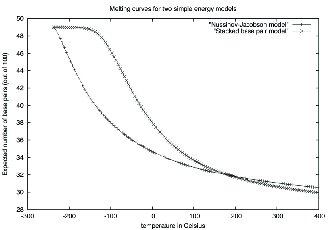
Figure 2. Theoretical melting curve for two simple energy models of RNA secondary structure. Temperature in Celsius is given on the $x$-axis, while expected number of base pairs is given on the $y$-axis. We implemented an algorithm, using dynamic programming, with run time $O(n^{5})$ and space $O(n^{3})$, to compute the partition function $Z_{k}=\sum_{S\in\mathbb{S}_{k}}\exp(-E(S)/RT)$, where $\mathbb{(}S)_{k}$ denotes the set of all secondary structures for a homopolymer of length 100 nt, having exactly $k$ base pairs. The expected number of base pairs is thus $\sum_{k}k\cdot p_{k}$, where $p_{k}=\frac{Z_{k}}{Z}$ denotes the probability that a secondary structure has $k$ base pairs, and $Z$ denotes the full partition function $Z=\sum_{S}\exp(-E(S)/RT)=\sum_{k}Z_{k}$. (Alternatively, and more simply, we could have produced this curve from the Taylor coefficients of the expressions to the right of the limit in equations (3) and(6), after first solving for $S(z,u)$ [resp. $S(z,u,v)$] in equation (1) [resp. (4)].) In the Nussinov-Jacobson energy model [28], $E(S)$ is defined to be $-1\cdot|S|$; i.e. $-1$ times the number of base pairs of $S$. In the base stacking energy model, $E(S)$ is defined to be $-1$ times the number of stacked base pairs of $S$. Although both models are quite similar, we see that the melting curves are indeed different, where the base stacking model entails more cooperative folding (see [6] for discussion of cooperative folding).

4. Enumeration of locally optimal secondary structures

4.1. Duality: RNA secondary structure $\leftrightarrow$ weighted plane tree

It is well known that secondary structures have a tree shape, and there are several ways to formulate it. Here we find convenient to associate in a bijective way to a secondary structure (in the homopolymer formulation) a rooted plane tree with nonnegative integers (weights) at the corners and at the edges. The transformation is shown in Figure 3. Start with a secondary structure $S$ of length $n$, the elements in the sequence being ranked from $1$ to $n$. Call segment of $S$ a sequence $i,i+1,\ldots,j$ such that $i<j$ and: (i) either $i=0$, or $1\leq i\leq n$ and the element $i$ is linked, (ii) either $j=n+1$, or $1\leq j\leq n$ and the element $j$ is linked, (iii) all elements in $i+1,\ldots,j-1$ are free. Note that there are $j-i-1$ free elements in the segment. Then perform two reduction operations on $S$:

Stem-reduction:

Replace each stem $\ell_{0},\ldots,\ell_{k}$ by a single link.

Segment-reduction:

Replace each segment by a unit segment (with no free element on it).

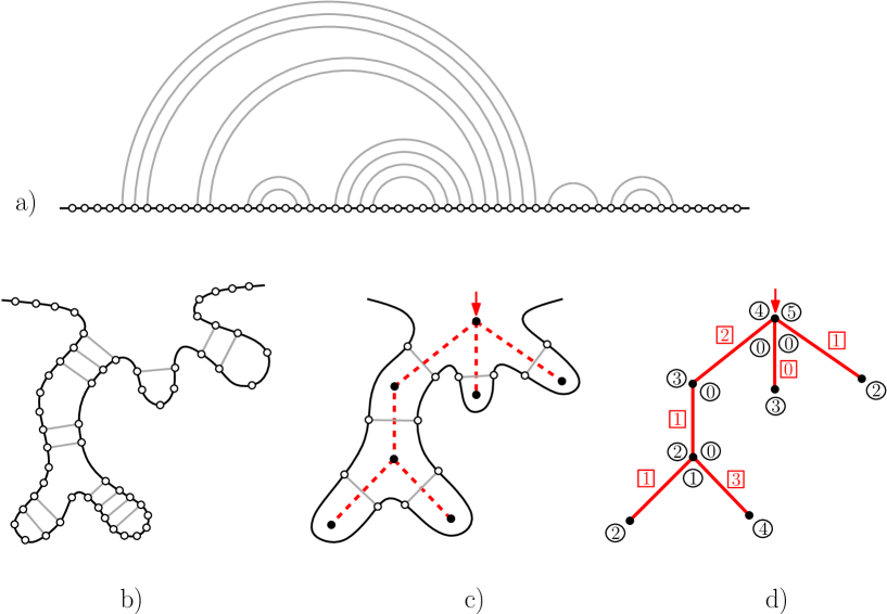
Figure 3. (a) A (homopolymer) secondary structure, (b) deformed into a tree-like shape, (c) the reduced structure superimposed with the dual rooted plane tree (in dashed lines, with the root indicated by an ingoing arrow), (d) the rooted plane tree with weights at corners (surrounded by circles) to indicate segment lengths, and weights at edges (surrounded by squares) to indicate stem lengths.

Call $R$ the reduced structure (which has no free element). Given the standard plane representation of $R$, draw a vertex, called a dual vertex in each region, and for each link of $R$, draw a dual edge connecting the vertices in the regions on each side of the link. The obtained figure (keeping the dual vertices and dual edges only) is a rooted plane tree $T$. Note that each edge of $T$ corresponds to a link of $R$ (hence corresponds to a stem of $S$), and each corner of $T$ corresponds to a segment of $S$. We weight $T$ by giving to each of its corners a weight corresponding to the number of free elements in the corresponding segment, and giving to each of its edges a weight corresponding to the length of the corresponding stem. Several parameters are in correspondence through the bijection (we use the standard terminology for parameters of secondary structures, a node of a tree is called a leaf if its arity is $0$ and an inner node if it has positive arity): See Table 1 for a summary of the correspondences between secondary structure loops and nodes of a weighted tree.

secondary structure $S$	$\leftrightarrow$	weighted tree $T$
hairpin	$\leftrightarrow$	leaf
bulge	$\leftrightarrow$	inner node with one child
multiloop	$\leftrightarrow$	inner node with several children
segment with $L$ free elements	$\leftrightarrow$	corner of weight $L$
stem of length $k$	$\leftrightarrow$	edge of weight $k$

Table 1. Correspondence between types of loop in secondary structure $S$ and types of node in the plane tree $T$ obtained by duality.

Note also that the number of links of $S$ is the number $|E|$ of edges plus the total weight $W_{e}$ over all edges, and that the number of free elements of $S$ is the total weight $W_{c}$ over all corners, hence the length $n$ of $S$ satisfies $n=2|E|+2W_{e}+W_{c}$.

A weighted rooted plane tree with at least one edge is called admissible if it corresponds to a valid secondary structure (which has at least one link), i.e., if the weights satisfy the following conditions:

1. Each non-root node with one child has at least one of its two incident corners of positive weight (otherwise the stem-reduction would not have been complete).

2. Each corner at a leaf has weight at least $\theta$ (to satisfy the $\theta$-threshold condition).

3. Each edge has weight at least $\tau$ (to satisfy the $\tau$-threshold condition).

4.2. Generating functions

For $r\geq 1$, a weighted combinatorial class indexed by $r$ parameters is a set $\mathcal{A}$ together with a weight-function $W$ from $\mathcal{A}$ to $\mathbb{R}$ and $r$ parameter-functions $P_{1},\ldots,P_{r}$ (one for each parameter) from $\mathcal{A}$ to $\mathbb{N}$ such that for any fixed integers $n_{1},\ldots,n_{r}$, the set of structures $\gamma\in\mathcal{A}$ such that $P_{1}(\gamma)=n_{1},\ldots,P_{r}(\gamma)=n_{r}$ is finite. This set is denoted $\mathcal{A}[n_{1},\ldots,n_{r}]$. The corresponding multivariate generating function is

(7) $$A(x_{1},\ldots,x_{r}):=\sum_{\gamma\in\mathcal{A}}x_{1}^{P_{1}(\gamma)}\cdots x_{r}^{P_{r}(\gamma)}W(\gamma).$$

We say that variable $x_{i}$ marks the parameter $P_{i}$, for $1\leq i\leq r$. We also use the notation

$$[x_{1}^{n_{1}}\ldots x_{r}^{n_{r}}]A(x_{1},\ldots,x_{r}):=\sum_{\gamma\in\mathcal{A}[n_{1},\ldots,n_{r}]}W(\gamma).$$

In general we consider enumerative generating functions, where $W(\cdot)$ assigns weight $1$ to each structure. However we allow ourselves to weight these structures, e.g., to weight each secondary structure by $p^{\#(\mathrm{links})}$, with $p$ a so-called stickiness parameter. The variables $x_{i}$ are a priori considered as formal, but one can also evaluate a generating function at given values, provided the sum converges. The convergence domain of $A(x_{1},\ldots,x_{r})$ is the set of $r$-tuples $(x_{1},\ldots,x_{r})$ of nonnegative real values such that $A(x_{1},\ldots,x_{r})$ converges.

As a first example, we briefly recall here how to enumerate (homopolymer) secondary structures, via the dual representation by weighted rooted plane trees and using generating functions. Let $\mathcal{F}$ be the family of rooted plane trees, possibly reduced to a single vertex, with some marked corners (to be occupied by positive weights later on) incident to inner nodes such that each node with one child has at least one marked corner. Let $F\equiv F(u,v,x)$ be the generating function of $\mathcal{F}$ where $u$ marks the number of leaves, $v$ marks the number of marked corners, and $x$ marks the number of edges. When the root-node $v$ has arity $1$, exactly one of its two corners is marked, hence the generating function for trees in $\mathcal{F}$ whose root-node has arity $1$ is $2vxF$. When the root-node $v$ has arity $k\geq 2$, there are $(k+1)$ corners incident to $v$, and each of these can be marked (independently). Hence the generating function for trees in $\mathcal{F}$ where the root-node has arity $k$ is $(1+v)^{k+1}x^{k}F^{k}$. Consequently, $F$ satisfies

(8) $$F=u+(2v+v^{2})xF+\sum_{k\geq 2}x^{k}(1+v)^{k+1}F^{k}=u+\frac{x(1+v)^{2}F}{1-x(1+v)F}-xF.$$

Let $\mathcal{G}$ be the family of rooted plane trees with at least one edge and with some marked corners (to be occupied by positive weights later on) incident to inner nodes such that each non-root node with one child has at least one marked corner. Let $G\equiv G(u,v,x)$ be the generating function of $\mathcal{G}$ where $u$ marks the number of leaves, $v$ marks the number of marked corners, and $x$ marks the number of edges. Again by decomposing at the root, we get

(9) $$G=\sum_{k\geq 1}x^{k}(1+v)^{k+1}F^{k}=\frac{x(1+v)^{2}F}{1-x(1+v)F}.$$

Let $g(t,s)$ be the series counting secondary structures with at least one link, where $t$ marks the number of free elements, and $s$ marks the number of links. Note that $g(t,s)$ is also the generating function of admissible rooted weighted plane trees where $t$ marks the total weight over corners, and $s$ marks the number of edges plus the total weight over edges. Such a tree is uniquely obtained from a tree in $\mathcal{G}$ where each corner at a leaf is assigned a weight of value at least $\theta$, each non-marked corner at an inner node is assigned weight $0$, each marked corner is assigned a positive weight, and each edge is assigned a weight of value at least $\tau$. Hence we have $g(t,s)=G(U,V,X)$, where

$$U:=\sum_{i\geq\theta}t^{i}=\frac{t^{\theta}}{1-t},\ V=\frac{t}{1-t},\ X:=s\sum_{i\geq\tau}s^{i}=\frac{s^{\tau+1}}{1-s}.$$

To summarize, we have an expression (written as a system of two equations) for the generating function $g(t,s)$ enumerating secondary structures with at least one link, where $t$ marks the number of free elements and $s$ marks the number of links (the generating function of all secondary structures, including the ones with no link, is clearly $g(t,s)+t+t^{2}+\cdots=g(t,s)+\frac{t}{1-t}$). Indeed, if we define $f(t,s):=F(U,V,X)$, then we easily see (since the substitutions of variables are rational expressions whose series-expansion have nonnegative coefficients) that there is a one-line equation specifying $f(t,s)$, of the form $f(t,s)=Q(t,s,f(t,s))$, with $Q\equiv Q(t,s,y)$ a rational expression whose series-expansion (in $s$, $t$, $y$) has nonnegative coefficients. And there is a rational expression $R\equiv R(t,s,y)$ whose series-expansion has nonnegative coefficients and such that $g(t,s)=R(t,s,f(t,s))$. Precisely

$$Q=\mathrm{substitute}\left(u=\frac{t^{\theta}}{1-t},v=\frac{t}{1-t},x=\frac{s^{\tau+1}}{1-s}\right)\ \ \mathrm{into}\ \ u+\frac{x(1+v)^{2}y}{1-x(1+v)y}-xy,$$

$$R=\mathrm{substitute}\left(v=\frac{t}{1-t},x=\frac{s^{\tau+1}}{1-s}\right)\ \ \mathrm{into}\ \ \frac{x(1+v)^{2}y}{1-x(1+v)y}.$$

This allows us to extract the counting coefficients. Let $g_{p}(t)$ be the weighted generating function of secondary structures where $t$ marks the length, and where each structure has weight $p^{\#(\mathrm{links})}$: $g_{p}(t)=g(t,pt^{2})+t/(1-t)$ (the term $t/(1-t)$ gathers secondary structures with no link); for instance for $\theta=1$ and $\tau=0$ we find

$$g_{p}(t)=t+t^{2}+(1+p)t^{3}+(1+3p)t^{4}+(1+6p+p^{2})t^{5}+(1+10p+6p^{2})t^{6}+(1+15p+20p^{2}+p^{3})t^{7}+\cdots.$$

4.3. Counting saturated structures

The Nussinov energy $E(S)$ of a secondary structure $S$ is defined as $E(S)=-L(S)$, with $L(S)$ the number of links in $S$. A secondary structure $S$ is called saturated (or locally optimal for the Nussinov energy) if it is not possible to add a link to $S$ (i.e., decrease the energy by $1$) while keeping a valid secondary structure.

Lemma 1.

Assume $\tau=0$ (no restriction on the lengths of stems). Saturated secondary structures with at least one link correspond to admissible weighted rooted plane trees such that:

• all corners have weight at most $\theta+1$,

• at each node there is at most one corner of strictly positive weight.

As shown in Figure 4, if there are two positive corners at the same inner node, then it is possible to add a link. Also, if there is a corner with weight at least $\theta+2$ then one can link the first and last free elements in the corresponding segment. Hence the weight of each corner is at most $\theta+1$. And these are the only two situations where it is possible to add a link without breaking planarity nor breaking the $\theta$-threshold condition. $\Box$

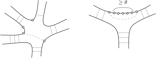
Figure 4. Situations where it is possible to add a link to a secondary structure.

Call $\mathcal{F}$ the family of rooted plane trees with some marked corners incident to inner nodes (these marked corners are to be occupied by positive weights later on) such that: (i) each node with one child has exactly one marked corner, (ii) each node with several children has at most one marked corner. Let $F\equiv F(u,v,x)$ be the generating function of $\mathcal{F}$ where $u$ marks the number of leaves, $v$ marks the number of marked corners, and $x$ marks the number of edges. When the root-node $v$ has arity $1$, exactly one of its two corners is marked, hence the generating function for trees in $\mathcal{F}$ whose root-node has arity $1$ is $2vxF$. When the root-vertex $v$ has arity $k\geq 2$, there are $(k+1)$ corners incident to $v$, and at most one of these corners has positive weight. Hence the generating function for trees in $\mathcal{F}$ where the root-vertex has arity $k$ is $(1+(k+1)v)x^{k}F^{k}$. Consequently, $F$ satisfies

$$F=u+2vxF+\sum_{k\geq 2}(1+(k+1)v)x^{k}F^{k},$$

Hence, using the identity $\sum_{k\geq 0}(k+1)A^{k}=1/(1-A)^{2}$, $F$ satisfies

(10) $$F=u+\frac{x^{2}F^{2}}{1-xF}+\frac{v}{(1-xF)^{2}}-v.$$

Now let $\mathcal{G}$ be the family of rooted plane trees with at least one edge, and with marked corners incident to inner nodes such that: (i’) each node $v$ with one child has exactly one marked corner if $v$ is different from the root-node, and has at most one marked corner if $v$ is the root-node, (ii) each node with several children has at most one marked corner. Let $G\equiv G(u,v,x)$ be the generating function of $\mathcal{G}$ where $u$, $v$, $x$ mark respectively the numbers of leaves, marked corners, and edges. Decomposing again at the root, we get

(11) $$G=\sum_{k\geq 1}(1+(k+1)v)x^{k}F^{k}=\frac{xF}{1-xF}+\frac{v}{(1-xF)^{2}}-v.$$

We take here $\tau=0$ (no restriction on the lengths of stems). Let $g(t,s)$ be the generating function of saturated secondary structures with at least one link, where $t$ marks the number of free elements and $s$ marks the number of links. Then Lemma 1 ensures that $g(t,s)=G(U,V,X)$, where

$$U=t^{\theta}(1+t),\ V=t+\ldots+t^{\theta+1}=\frac{t-t^{\theta+2}}{1-t},\ X=\frac{s}{1-s}.$$

To summarize (in a similar way as for general structures), we have an expression (written as a system of two equations) for the generating function $g(t,s)$ enumerating saturated secondary structures with at least one link, where $t$ marks the number of free elements and $s$ marks the number of links (the generating function of all saturated secondary structures, including the ones with no link, is $g(t,s)+t+\cdots+t^{\theta+1}=g(t,s)+\frac{t-t^{\theta+2}}{1-t}$). Indeed, if we define $f(t,s):=F(U,V,X)$, then there is a one-line equation specifying $f(t,s)$, of the form $f(t,s)=Q(t,s,f(t,s))$, with $Q(t,s,y)$ a rational expression whose series-expansion (in $s$, $t$, $y$) has nonnegative coefficients. And there is a rational expression $R(t,s,y)$ whose series-expansion has nonnegative coefficients and such that $g(t,s)=R(t,s,f(t,s))$. Precisely

$$Q=\mathrm{substitute}\left(u=t^{\theta}(1+t),v=\frac{t-t^{\theta+2}}{1-t},x=\frac{s}{1-s}\right)\ \ \mathrm{into}\ \ u+\frac{x^{2}y^{2}}{1-xy}+\frac{v}{(1-xy)^{2}}-v,$$

$$R=\mathrm{substitute}\left(v=\frac{t-t^{\theta+2}}{1-t},x=\frac{s}{1-s}\right)\ \ \mathrm{into}\ \ \frac{xy}{1-xy}+\frac{v}{(1-xy)^{2}}-v.$$

Again this allows us to extract the counting coefficients. Let $g_{p}(t)$ be the weighted generating function of saturated secondary structures where $t$ marks the length, and where each structure has weight $p^{\#(\mathrm{links})}$: $g_{p}(t)=g(t,pt^{2})+t+\cdots+t^{\theta+1}$; for $\theta=1$ and $\tau=0$ we find

$$g_{p}(t)=t+t^{2}+pt^{3}+3pt^{4}+(4p+p^{2})t^{5}+(2p+6p^{2})t^{6}+(17p^{2}+p^{3})t^{7}+\cdots.$$

4.4. Counting G-saturated structures

The base stacking energy $E(S)$ of a secondary structure $S$ is defined as $E(S):=-T(S)$, with $T(S)$ the sum of sizes of all stems of $S$. A (homopolymer) secondary structure is called G-saturated (locally optimal for the base stacking energy) if it is not possible to add a link so as to extend a stem (i.e., decrease by $1$ the base stacking energy). In general, the addition of a link to a secondary structure either creates a new stem of length $0$ or extends an already existing stem. Hence, in a G-saturated structure a valid link addition always creates a new stem of length $0$. In case $\tau>0$, creating a stem of length $0$ is not a valid link addition (since the stems must have positive length), hence no valid link addition to a G-saturated is possible for $\tau>0$. In other words, the concepts of saturated and of G-saturated structures coincide when $\tau>0$ (whereas for $\tau=0$ the class of saturated structures is strictly contained in the class of G-saturated structures). In this section we enumerate G-saturated structures according to the number of free elements and the number of links, for any given values of the threshold parameters $\tau$ and $\theta$.

Again we formulate the conditions on the dual representation. For this purpose we define adjacency of corners. Two corners $c$ and $c^{\prime}$ of a rooted plane tree $T$ are called adjacent if they are incident to the same vertex $v$ of $T$ and there is an edge $e$ incident to $v$ such that $c$ and $c^{\prime}$ are the corners incident to $v$ on each side of $e$. Note that the two corners on each side of the root (the root is represented as an ingoing arrow in Figure 3) are considered as adjacent only when the root-node $v$ has arity $1$ (in which case they are adjacent through the unique edge incident to $v$).

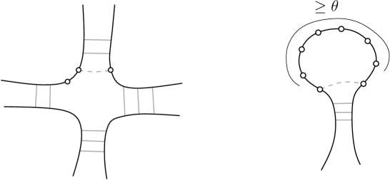
Figure 5. Situations where it is possible to extend a stem of a secondary structure.

Lemma 2.

The G-saturated secondary structures with at least one link correspond to admissible weighted rooted plane trees such that:

• the corners at leaves have weight at most $\theta+1$,

• any two adjacent corners can not both have strictly positive weight.

As shown in Figure 5, if there are two adjacent positive corners, then it is possible to add a link so as to extend an existing stem. Also, if there is a corner of weight at least $\theta+2$ at a leaf $\ell$, then one can link the first and last free elements in the corresponding segment and thus extend the stem associated to the edge leading to $\ell$. Hence the weight of a corner at a leaf is at most $\theta+1$. And these are the only two situations where it is possible to extend a stem without breaking planarity nor breaking the $\theta$-threshold and $\tau$-threshold condition. $\Box$

Call $\mathcal{F}$ the family of rooted plane trees with some marked corners incident to inner nodes (again these marked corners are to be occupied by positive weights later on) such that: (i) each inner node with one child has exactly one marked corner, (ii) two corners can not both be marked if they are adjacent or if they are the two corners on each side of the root (the root is indicated by an ingoing arrow in Figure 3). Let $F\equiv F(u,v,x)$ be the generating function of $\mathcal{F}$ where $u$ marks the number of leaves, $v$ marks the number of marked corners, and $x$ marks the number of edges. Finding an equation satisfied by $F$ is a little more involved than for saturated structures. At first we need a preliminary study on independent sets (i.e., sets containing only pairwise non-adjacent elements) on a $k$-sequence or on a $k$-cycle.

For $k>0$ and $m\leq k$, let $c_{k,m}$ (resp. $s_{k,m}$) be the number of ways of choosing $m$ marked elements on the oriented cycle $(1,2,\ldots,k)$ (resp. sequence $1,2,\ldots,k$) of $k$ elements such that no two consecutive elements are marked, and let $C_{k}=C_{k}(v):=\sum_{m}c_{k,m}v^{m}$ (resp. $S_{k}=S_{k}(v):=\sum_{m}s_{k,m}v^{m}$) be the corresponding (polynomial) generating function. The polynomials $S_{k}$ are well-known to be the Fibonacci polynomials and satisfy an easy recurrence which we briefly recompute here. We take the convention $S_{0}=1$. Let $k\geq 2$. If an independent set on the $k$-sequence starts with a marked element, then the next element is forbidden and the remaining $(k-2)$-sequence might be occupied by any independent set; this gives a contribution $vS_{k-2}$ in $S_{k}$, where the factor $v$ takes account of the first element being marked. If an independent set on the $k$-sequence starts with a non-marked element, then the remaining $(k-1)$-sequence might be occupied by any independent set; this gives a contribution $S_{k-1}$ in $S_{k}$. Therefore

$$S_{k}=vS_{k-2}+S_{k-1}\ \ \mathrm{for}\ k\geq 2,\ \ S_{0}=1,\ S_{1}=1+v.$$

Now define $S\equiv S(v,z):=\sum_{k\geq 0}S_{k}(v)z^{k}$. The recurrence on $S_{k}$ above multiplied by $z^{k}$ and summed over $k\geq 2$ yields $S-S_{0}-zS_{1}=vz^{2}S+z(S-S_{0})$. With $S_{0}=1$ and $S_{1}=1+v$ we obtain

$$S=\frac{1+vz}{1-z-vz^{2}}.$$

Let us go back to independent sets on the $k$-cycle $(1,\ldots,k)$, for $k\geq 3$. In such a set, either $1$ is occupied, in which case the adjacent elements $2$ and $k$ are unoccupied and the remaining segment $3,\ldots,k-1$ might be occupied by any independent set. This gives contribution $vS_{k-3}$ to $C_{k}$. If $1$ is unoccupied, then the remaining segment $2,\ldots,k$ might be occupied by any independent set; this gives contribution $S_{k-1}$ to $C_{k}$. Consequently

$$C_{k}=vS_{k-3}+S_{k-1}\ \ \mathrm{for}\ k\geq 3.$$

If the root-node $v$ of a tree in $\mathcal{F}$ has arity $1$ then exactly one of its two incident corners is marked (by definition of $\mathcal{F}$), thus the generating function of trees in $\mathcal{F}$ whose root-node has arity $1$ is $2vxF$; if $v$ has arity $k\geq 2$ then the marked corners around $v$ form an independent set (no two consecutive corners are marked). Thus, for $k\geq 2$, the generating function of trees in $\mathcal{F}$ whose root-node has arity $k$ is $C_{k+1}(v)x^{k}F^{k}$ (since there are $k+1$ corners incident to the root-node). Consequently $F$ satisfies

$$F = u+2vxF+\sum_{k\geq 2}C_{k+1}(v)x^{k}F^{k}$$

$$= u+2vxF+\sum_{k\geq 2}\big{[}vS_{k-2}+S_{k}\big{]}x^{k}F^{k}$$

$$= u+2vxF+vx^{2}F^{2}S(v,xF)+\big{(}S(v,xF)-1-(1+v)xF\big{)}.$$

Using the rational expression of $S$ above and rearranging, we obtain

(12) $$F=u+2vxF+\frac{1+2vx^{2}F^{2}\cdot(1+vxF)}{1-xF-vx^{2}F^{2}}-xF-1.$$

Now let $\mathcal{G}$ be the family of rooted plane trees with at least one edge and where some corners at inner nodes are marked such that (i) each non-root inner node of arity $1$ has exactly one marked corner, (ii) two adjacent corners can not both be marked. And let $G\equiv G(u,v,x)$ be the generating function of $\mathcal{G}$ where $u$ marks the number of leaves, $v$ marks the number of marked corners, and $x$ marks the number of edges. The difference between $\mathcal{G}$ and $\mathcal{F}$ is at the root-vertex: in $\mathcal{G}$ the two corners on each side of the root are allowed to be both marked when the root-vertex has more than one child, and are allowed to be both unmarked when the root-vertex has one child. So we have

$$G=\sum_{k\geq 1}S_{k+1}(v)x^{k}F^{k}.$$

Using the rational expression of $S$ above and rearranging, we obtain the following expression for $G$ in terms of $F$:

(13) $$G=\frac{xF(1+2v+(1+v)vxF)}{1-xF-vx^{2}F^{2}}.$$

Now let $g(t,s)$ be the generating function of G-saturated structures with at least one link, where $t$ marks the number of free elements and $s$ marks the number of links. By Lemma 2,

(14) $$g(t,s)=G(U,V,X),$$

where

$$U=t^{\theta}(1+t),\ \ V=\frac{t}{1-t},\ \ X=\frac{s^{\tau+1}}{1-s}.$$

The conclusion is similar to the other two cases (general structures, saturated structures): we have an expression (written as a system of two equations) for the generating function $g(t,s)$ enumerating G-saturated secondary structures with at least one link, where $t$ marks the number of free elements and $s$ marks the number of links (the generating function of all G-saturated secondary structures, including the ones with no link, is $g(t,s)+t+t^{2}+\cdots=g(t,s)+\frac{t}{1-t}$). Indeed, if we define $f(t,s):=F(U,V,X)$, then there is a one-line equation specifying $f(t,s)$, of the form $f(t,s)=Q(t,s,f(t,s))$, with $Q(t,s,y)$ a rational expression whose series-expansion (in $s$, $t$, $y$) has nonnegative coefficients. And there is a rational expression $R(t,s,y)$ whose series-expansion has nonnegative coefficients and such that $g(t,s)=R(t,s,f(t,s))$. Precisely

$$Q=\mathrm{substitute}\left(u=t^{\theta}(1+t),v=\frac{t}{1-t},x=\frac{s^{\tau+1}}{1-s}\right)\ \ \mathrm{into}\ \ u+2vxy+\frac{1+2vx^{2}y^{2}(1+vxy)}{1-xy-vx^{2}y^{2}}-1-xy,$$

$$R=\mathrm{substitute}\left(v=\frac{t}{1-t},x=\frac{s^{\tau+1}}{1-s}\right)\ \ \mathrm{into}\ \ \frac{xy(1+2v+(1+v)vxy)}{1-xy-vx^{2}y^{2}}.$$

Again this allows us to extract the counting coefficients. Let $g_{p}(t)$ be the weighted generating function of G-saturated secondary structures where $t$ marks the length, and where each structure has weight $p^{\#(\mathrm{links})}$: $g_{p}(t)=g(t,pt^{2})+t/(1-t)$; for $\theta=1$ and $\tau=0$ we find

$$g_{p}(t)=t+t^{2}+(1+p)t^{3}+(1+3p)t^{4}+(1+4p+p^{2})t^{5}+(1+4p+6p^{2})t^{6}+(1+4p+17p^{2}+p^{3})t^{7}+\cdots.$$

5. Asymptotic results

5.1. Asymptotic enumeration

We show here that the number of structures of length $n$ follows a universal asymptotic behaviour in $c\ \!\gamma^{n}n^{-3/2}$ (with $c$ and $\gamma$ explicit positive constants), which is typical of tree-structures. The proof classically relies on the Drmota-Lalley-Woods theorem [11, VII.6], which we recall at first. Consider an equation of the form

(15) $$a(t)=\Phi(t,a(t)),$$

where $\Phi(t,y)$ is a rational expression in $t$ and $y$. Such an equation is called admissible if the following conditions are satisfied:

• the rational expression $\Phi(t,y)$ has a series-expansion in $t$ and $y$ with nonnegative coefficients, is nonaffine in $y$, and satisfies  $\Phi(0,0)=0$ and $\Phi_{y}(0,0)=0$,

• the unique generating function $y=a(t)$ solution of (15) is aperiodic, i.e., can not be written as $a(t)=t^{q}\tilde{a}(t^{p})$ for some integers $p,q$ with $p\geq 2$.

There is an easy criterion to check the aperiodicity condition: it suffices to prove that there is some $n_{0}$ such that $[t^{n}]a(t)>0$ for $n\geq n_{0}$.

Theorem 3 (Drmota-Lalley-Wood).

Let $y=a(t)$ be the generating function that is the unique solution of an admissible equation $y=\Phi(t,y)$. Then

$$[t^{n}]a(t)\sim c\ \!\gamma^{n}\ \!\!n^{-3/2},$$

where $\gamma=1/t_{0}$, with $(t_{0},y_{0})$ the unique pair in the convergence domain of $\Phi(t,y)$ that is solution of the singularity system:

$$y=\Phi(t,y),\ \ \ \Phi_{y}(t,y)=1;$$

and where

$$c=\sqrt{t_{0}\Phi_{t}(t_{0},y_{0})/(2\pi\Phi_{y,y}(t_{0},y_{0}))}.$$

Moreover, if $\Psi(t,y)$ is a rational expression not constant in $y$, that has a series-expansion with nonnegative coefficients, and such that the convergence domain of $\Psi(t,y)$ is contained in the convergence domain of $\Phi(t,y)$, then the coefficients of the generating function $b(t):=\Psi(t,a(t))$ behave as

$$[t^{n}]b(t)\sim d\ \!\gamma^{n}\ \!\!n^{-3/2},$$

where $d=c\cdot\Psi_{y}(t_{0},y_{0})$.

Remark 1.

The Drmota-Lalley-Wood theorem is classically proved (e.g. in [11, VII.6]) for polynomial systems (i.e., for $\Phi(t,y)$ a polynomial). But one easily checks that, more generally, if $\Phi(t,y)$ is a bivariate series that diverges at all its singularities, then the conclusions remain the same.

From the Drmota-Lalley-Wood theorem we obtain

Proposition 1.

Let $p$ be a fixed positive real value (stickiness parameter). Let $g_{p}(t)$ be the univariate generating function of general (resp. saturated, resp. G-saturated) homopolymer secondary structures, where $t$ marks the length of the sequence and where each structure has weight $p^{\#(\mathrm{links})}$.

Then, for any values of the threshold-parameters $\theta$ and $\tau$ ($\tau=0$ if one considers saturated structures), there are computable positive constants $c$ and $\gamma$ (depending on $\tau$, $\theta$, $p$, and in which setting: general, saturated, or G-saturated) such that

$$[t^{n}]g_{p}(t)\sim c\ \!\gamma^{n}\ \!\!n^{-3/2}.$$

Recall that, in each of the three settings (general, saturated, G-saturated), $g(t,s)$ denotes the generating function of secondary structures with at least one link, where $t$ marks the number of free elements and $s$ marks the number of links. We have seen that, in each of the three settings, there are two rational expressions $Q(t,s,y)$ and $R(t,s,y)$ that have nonnegative coefficients (in the series-expansion), and there is an adjoint generating function $f(t,s)$ such that $f(t,s)=Q(t,s,f(t,s))$ and $g(t,s)=R(t,s,f(t,s))$. In addition, the convergence domain of $Q(t,s,y)$ is clearly the same as the convergence domain of $R(t,s,y)$; for instance, for G-saturated structures, the convergence domain is the set of nonnegative triples $(t,s,y)$ such that $t<1$, $s<1$, and $xy+vx^{2}y^{2}<1$, where $v=t/(1-t)$ and $x=s^{\tau+1}/(1-s)$. Note that in all three settings, $f(0,0)=1$ for $\theta=0$ and $f(0,0)=0$ for $\theta>0$. If we set $a(t):=f(t,pt^{2})-\mathbf{1}_{\theta=0}$ (with $\theta$ the threshold parameter) and $b(t):=g(t,pt^{2})$, then we are in the conditions of the Drmota-Lalley-Wood theorem, with $\Phi(t,y):=Q(t,pt^{2},y+\mathbf{1}_{\theta=0})-\mathbf{1}_{\theta=0}$ and $\Psi(t,y):=R(t,pt^{2},y+\mathbf{1}_{\theta=0})$. The conditions for $\Phi$ and $\Psi$ are readily checked, we show now the aperiodicity of $a(t):=f(t,pt^{2})$ (proving that the $n$th coefficient is strictly positive for $n$ large enough). Note that it is enough to consider $p=1$ (the strict positivity of $[t^{n}]f(t)$ does not depend on $p>0$). In each of the three settings (general, saturated, G-saturated), $a(t)$ is the enumerative generating function of some explicit class of rooted weighted plane trees. For instance, for saturated structures, $a(t)$ counts admissible rooted weighted plane trees with all corners of weight at most $\theta+1$, with at most one positive corner per node, and where each node of arity $1$ has exactly one positive corner. For $i\geq\tau$, consider the weighted rooted plane tree $T_{i}$ made of one edge $e$ leading to a leaf $\ell$, with weight $1$ (resp. $0$) at the corner to the left (resp. right) of the root, with weight $i$ on $e$ and weight $\theta$ on $\ell$. And consider the tree $T_{i}^{\prime}$ defined exactly as $T_{i}$ except that $\ell$ has weight $\theta+1$. Note that $T_{i}$ contributes to $[t^{2i+\theta+3}]a(t)$ and $T_{i}^{\prime}$ contributes to $[t^{2i+\theta+4}]a(t)$. Hence $[t^{n}]a(t)>0$ for all $n\geq 2\tau+\theta+3$, so $a(t)$ is aperiodic. In exactly the same way, $a(t)$ is aperiodic in the general setting and in the G-saturated setting.

Theorem 3 ensures that there are $c>0$ and $\gamma>0$ such that $[t^{n}]g(t,pt^{2})\sim c\gamma^{n}\ \!n^{-3/2}$. Actually, in the case of general and G-saturated structures, we have $\gamma>1$ since (according to Theorem 3) there is some $y_{0}$ such that $(1/\gamma,y_{0})$ is in the convergence domain of $\Phi(t,y)$, and since clearly any $(t_{0},y_{0})$ in the convergence domain of $\Phi(t,y)$ satisfies $t_{0}<1$ (indeed $Q(t,s,y)$ involves the quantity $1/(1-t)$, in each of the general and in the G-saturated case). The generating function $g_{p}(t)$ (which includes also secondary structures with no link, as opposed to $g(t,s)$) satisfies $g_{p}(t)=g(t,pt^{2})+t/(1-t)$ for secondary and for G-saturated structures, and satisfies $g_{p}(t)=g(t,pt^{2})+t+\ldots+t^{\theta+1}$ for saturated structures. So the additional term gathering saturated structures with no link has negligible asymptotic contribution in all cases. $\Box$

For $p=1$, $g_{p}(t)$ is the enumerative generating function of homopolymer structures. Another value of interest is $p=3/8$. Indeed, if we want to count RNA secondary structures (each base is labelled by a letter in $\{A,G,C,U\}$) instead of homopolymers, this corresponds to giving weight $4$ to each free element (because there are $4$ possible labels) and giving weight $6$ to each pair of linked elements (because there are $6$ allowed labellings out of $4^{2}=16$, due to the Watson-Crick and wobble pairs). Therefore the corresponding enumerative generating function is $g(4t,6t^{2})$. We have

$$[t^{n}]g(4t,6t^{2})=4^{n}[t^{n}]g(t,3t^{2}/8)=4^{n}[t^{n}]g_{3/8}(t).$$

In other words, $[t^{n}]g_{3/8}$ is the expected number of RNA secondary structures with the desired properties (general, saturated, or G-saturated) on a random sequence of size $n$ (i.e., for a random word in $\{A,G,C,U\}^{n}$).

Table 2 shows the asymptotic behaviour of $[t^{n}]g_{p}(t)$ for $p=1$ and $p=3/8$ in the three settings. (The methodology to compute $\gamma$ for saturated structures using computer algebra tools is detailed in [5].)

Table 2. Asymptotic behaviour of the $n$th coefficient of the generating function $g_{p}(t)$ counting secondary structures (general, saturated, or G-saturated) with weight $p$ on each link.

5.2. Limit law for the number of links

Using a theorem of Drmota [7] (closely related to the Drmota-Lalley-Wood theorem) we show that the number of links in a random secondary structure (general, saturated, or G-saturated) of length $n$ is asymptotically a gaussian law with $\Theta(n)$ expectation and $\Theta(\sqrt{n})$ standard deviation.

Consider an equation of the form

(16) $$a(t,u)=\Phi(t,u,a(t,u)),$$

where $\Phi(t,u,y)$ is a rational expression in $t$, $u$ and $y$. Such an equation is called admissible if $\Phi(t,u,y)$ is nonconstant in $u$, has a series-expansion (in $t$, $u$, $y$) with nonnegative coefficients, the equation $y=\Phi(t,1,y)$ is admissible (in the sense of Section 5.1), and there is a $3\times 3$-matrix $m[i,j]$ with integer coefficients and nonzero determinant such that $[t^{m[i,1]}u^{m[i,2]}y^{m[i,3]}]\Phi(t,u,y)>0$ for all $i\in\{1,2,3\}$.

Theorem 4 (Drmota [7]).

Let $y=a(t,u)$ be a generating function that is the unique solution of an admissible equation $y=\Phi(t,u,y)$. Assume that the generating function $b(t,u)=\sum_{\gamma\in\mathcal{G}}t^{|\gamma|}u^{\chi(\gamma)}W(\gamma)$ of a weighted combinatorial class $\mathcal{G}$ is given by $b(t,u)=\Psi(t,u,a(t,u))$, with $\Psi(t,u,y)$ a rational expression with nonnegative coefficients (in the series-expansion), nonconstant in $y$, and such that the convergence domain of $\Psi(t,1,y)$ is included in the one of $\Phi(t,1,y)$. For $n\geq 0$ let $\mathcal{G}_{n}:=\{\gamma\in\mathcal{G},\ |\gamma|=n\}$, and define the random variable $X_{n}$ as $\chi(\gamma)$, with $\gamma$ a random structure in $\mathcal{G}_{n}$ under the distribution

$$P(\gamma)=\frac{W(\gamma)}{\sum_{\gamma\in\mathcal{G}_{n}}W(\gamma)}.$$

For $u>0$ in a neighbourhood of $1$, denote by $\rho(u)$ the radius of convergence of $y:t\to a(t,u)$, and let

$$\mu=-\frac{\rho^{\prime}(1)}{\rho(1)},\ \ \ \sigma^{2}=-\frac{\rho^{\prime\prime}(1)}{\rho(1)}-\frac{\rho^{\prime}(1)}{\rho(1)}+\left(\frac{\rho^{\prime}(1)}{\rho(1)}\right)^{2}.$$

Then $\mu$ and $\sigma$ are strictly positive and $\displaystyle\frac{X_{n}-\mu\cdot n}{\sigma\sqrt{n}}$ converges as a random variable to a normal (gaussian) law.

Remark 2.

Again the theorem was originally proved for polynomial systems, but the arguments of the proof hold more generally when $\Phi$ is rational. The role of the condition involving the existence of a nonsingular $3\times 3$ matrix is to grant the strict positivity of $\sigma$, as recently proved in [8].

Table 3. Asymptotic behaviour of the number of links ($\mathcal{N}$ denotes a normal gaussian law).

Proposition 2.

Let $p>0$. For $n\geq 1$, let $X_{n}$ be the number of links in a general (resp. saturated, resp. G-saturated) secondary structure of length $n$ taken at random with weight proportional to $p^{\#(\mathrm{links})}$ (uniformly at random when $p=1$). Then there are computable strictly positive constants $\mu$ and $\sigma$ (depending on $p$, $\theta$, $\tau$, and on which setting: general, saturated, or G-saturated) such that $\frac{X_{n}-\mu\cdot n}{\sigma\sqrt{n}}$ converges as a random variable to a normal (gaussian) law.

In each of the three settings (general, saturated, G-saturated), we have called $g(t,s)$ the enumerative generating function of secondary structures with at least one link. We have seen that there are two rational expressions $Q(t,s,y)$ and $R(t,s,y)$ that have nonnegative coefficients (in the series-expansion), and there is an adjoint generating function $f(t,s)$ such that $f(t,s)=Q(t,s,f(t,s))$ and $g(t,s)=R(t,s,f(t,s))$; and the convergence domain of $Q(t,s,y)$ is the same as the convergence domain of $R(t,s,y)$. Note that the bivariate series $g(t,put^{2})$ (with variables $t$ and $u$) is the weighted generating function of secondary structures (with at least one link) where $t$ marks the length, $u$ marks the number of links, and where each structure has weight $p^{\#(\mathrm{links})}$. It is easily checked that, if we set $a(t,u):=f(t,put^{2})-\mathbf{1}_{\theta=0}$ (with $\theta$ the threshold parameter) and $b(t):=g(t,put^{2})$, then we are in the conditions of Theorem 4, with $\Phi(t,u,y):=Q(t,put^{2},y+\mathbf{1}_{\theta=0})-\mathbf{1}_{\theta=0}$ and $\Psi(t,u,y):=R(t,put^{2},y+\mathbf{1}_{\theta=0})$. Indeed the $3\times 3$ matrix condition is readily checked, and for $u=1$ we get the equation of Proposition 1, where we have already checked that the conditions are satisfied. $\Box$

Table 3 shows the asymptotic behaviour for some standard parameter values. (The methodology to compute $\mu$ for saturated structures using computer algebra tools is detailed in [5].) The case $p=1$ corresponds to a homopolymer of length $n$ taken uniformly at random, while the case $p=3/8$ corresponds to a (uniformly) random secondary structure where the underlying sequence is (any word) in $\{A,G,C,U\}^{n}$. As expected, saturated structures tend to have more links than G-saturated structures, which tend to have more links than general structures.

6. Inclusion of dangles

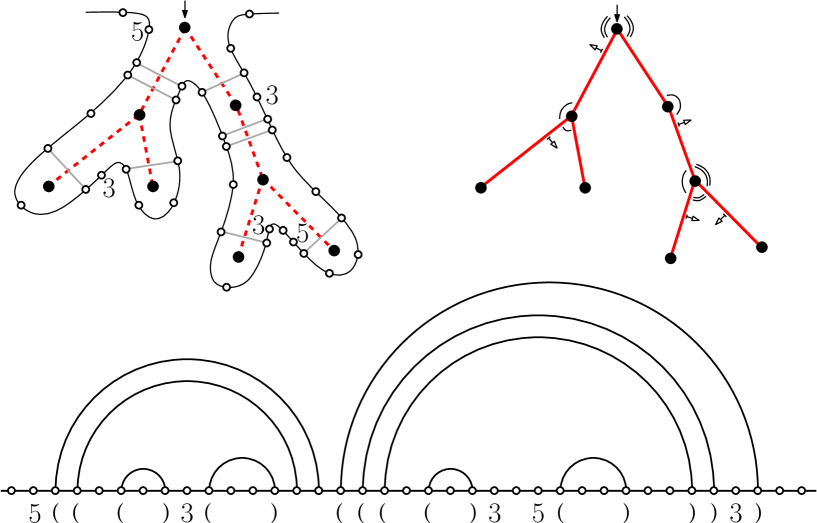
Figure 6. Bottom: a secondary structure with dangles (two $5^{\prime}$-dangles and three $3^{\prime}$-dangles). Top-left: the secondary structure with the dual plane tree. Top-right: each dangle yields a marked edge-side in the dual plane tree (corners at inner nodes are simply marked if they have weight $1$, are doubly marked if they have weight greater than $1$).

We show here that the counting approach developed so far (based on duality with plane trees, generating functions, and substitution operations) can be easily adapted to take the presence of so-called dangling bases into account. In the parenthesis representation of the secondary structure (see Figure 6, bottom) a dangling base (shortly dangle) is a distinguished free base of two possible kinds: a $5$-dangle has to be just before an opening parenthesis, a $3^{\prime}$-dangle has to be just after of a closing parenthesis. Note that a dangling base that is just before an opening parenthesis and just after a closing parenthesis is either a $5^{\prime}$-dangle or a $3^{\prime}$-dangle but not both. For a structure with dangling bases, the underlying secondary structure is the structure where dangling bases are considered as usual free bases (i.e., are not distinguished).

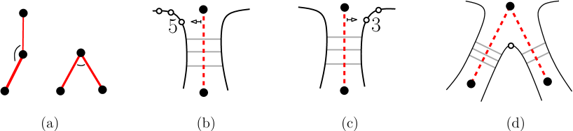
Figure 7. (a) The first drawing shows a lateral corner, the second drawing shows an extremal corner (depending edges are bolder). (b) A $5^{\prime}$-dangle yields a marked left-side of edge in the dual tree. (c) A $3^{\prime}$-dangle yields a marked right-side of edge in the dual tree. (d) Situation of an extremal corner of weight 1, in which case the two depending edge-sides can not both be marked.

In the dual plane tree, a $5^{\prime}$-dangle (resp. a $3^{\prime}$-dangle) is indicated by a marked edge-side to the left (resp. to the right) of the edge, see Figure 7(b)-(c). To take dangles into account in our counting method, we need to distinguish two types of corners in the dual plane tree $T$: a corner $c$ at vertex $v$ is called lateral if $c$ is incident to the edge going to the parent of $v$ in $T$ (when $v$ is not the root-vertex) or $c$ is incident to the root (when $v$ is the root-node); note that every inner node has two incident lateral corners (one on the left side, one on the right side). The other corners at inner nodes in the tree are called extremal, see Figure 7(a). Given a corner $c$ of $T$ (at an inner node), an edge-side $s$ incident to $c$ is said to depend on $c$ if $c$ is incident to $s$ at the extremity of $s$ closest to the root; note that a lateral corner has one depending edge-side while an extremal corner has two depending edge-sides, see Figure 7(a).

We now make important observations to determine when the edge-sides depending on a corner $c$ can be marked. If $c$ has weight $0$ then none of the depending edge-sides can be marked, because there is no free base in the sector of $c$ (hence no candidate to become a dangle). If $c$ is lateral and has positive weight (i.e., is a marked corner) then the depending edge-side is allowed to be marked. If $c$ is extremal of weight $1$ then at most one of the two edge-sides depending on $c$ is allowed to be marked (because the unique free base in the sector of $c$ can not be both a $5^{\prime}$-dangle and a $3^{\prime}$-dangle). If $c$ is extremal of weight at least $2$ then the two depending edge-sides are allowed to be marked (and are allowed to be both marked).

Given these observations we can easily include a variable for dangles in our generating function expressions (recall we have treated $3$ cases: general, saturated, G-saturated).

General structures, inclusion of dangles in the results of Section 4.2. Denote by $F\equiv F(u,v_{1},v_{2},x)$ the generating function of $\mathcal{F}$ (the one defined in Section 4.2) where $u$ marks the number of leaves, $v_{1}$ (resp. $v_{2}$) marks the number of marked corners that are lateral (resp. extremal), and $x$ marks the number of edges. Since a tree-vertex with $k\geq 1$ children has two incident corners that are lateral (the $k-1$ other ones are extremal), we get the following equation (which specifies $F$ uniquely):

$$F = u+(2v_{1}+v_{1}^{2})xF+\sum_{k\geq 2}x^{k}(1+v_{1})^{2}(1+v_{2})^{k-1}F^{k}$$

$$= u+\frac{x(1+v_{1})^{2}F}{1-x(1+v_{2})F}-xF.$$

Similarly, denoting by $G\equiv G(u,v_{1},v_{2},x)$ the generating function of $\mathcal{G}$ (where the variables have the same meaning as for $F$), we have

$$G=\frac{x(1+v_{1})^{2}F}{1-x(1+v_{2})F}.$$

Let $g(t,s,r)$ be the generating function counting secondary structures with at least one link, where $t$ marks the number of free elements (including dangles), $s$ marks the number of edges, and $r$ marks the number of dangles. Then $g(t,s,r)=G(U,V_{1},V_{2},X)$, where

$$U=\frac{t^{\theta}}{1-t},\ \ V_{1}=\frac{t(1+r)}{1-t},\ \ V_{2}=\frac{t(1+r)^{2}}{1-t}-tr^{2},\ \ X=\frac{s^{\tau+1}}{1-s}.$$

For $p>0,q\geq 0$, let $g_{p,q}(t)$ be the weighted generating function of secondary structures where each structure has weight $p^{\#(\mathrm{links})}q^{\#(\mathrm{dangles})}$. Then $g_{p,q}(t)=g(t,pt^{2},q)+t/(1-t)$. For instance, for $\theta=1$ and $\tau=0$ we find

$$g_{p,q}(t)=t+t^{2}+(1+p)t^{3}+(1+3p+2pq)t^{4}+(1+6p+p^{2}+6pq+pq^{2})t^{5}+\cdots.$$

Saturated structures, inclusion of dangles in the results of Section 4.3. The equation for $F$ obtained in Section 4.3 becomes (when splitting $v$ into two variables $v_{1},v_{2}$ respectively for lateral and extremal marked corners):

$$F = u+2v_{1}xF+\sum_{k\geq 2}(1+2v_{1}+(k-1)v_{2})x^{k}F^{k}$$

$$= u+\frac{x^{2}F^{2}+2xF\cdot(v_{1}-v_{2})}{1-xF}+\frac{v_{2}}{(1-xF)^{2}}-v_{2},$$

and the expression of $G$ becomes

$$G = \sum_{k\geq 1}(1+2v_{1}+(k-1)v_{2})x^{k}F^{k}$$

$$= \frac{xF\cdot\big{(}1+2(v_{1}-v_{2})\big{)}}{1-xF}+\frac{v_{2}}{(1-xF)^{2}}-v_{2}.$$

A structure with dangles is called saturated if the underlying secondary structure is saturated. Let $g(t,s,r)$ be the generating function counting saturated structures with at least one link, where $t$ marks the number of free elements (including dangles), $s$ marks the number of edges, and $r$ marks the number of dangles. Then $g(t,s,r)=G(U,V_{1},V_{2},X)$, where

$$U=t^{\theta}(1+t),\ \ V_{1}=\frac{t-t^{\theta+2}}{1-t}(1+r),\ \ V_{2}=\frac{t-t^{\theta+2}}{1-t}(1+r)^{2}-tr^{2},\ \ X=\frac{s}{1-s}.$$

For $p>0,q\geq 0$, let $g_{p,q}(t)$ be the weighted generating function of saturated structures where each structure has weight $p^{\#(\mathrm{links})}q^{\#(\mathrm{dangles})}$. Then $g_{p,q}(t)=g(t,pt^{2},q)+t+\cdots+t^{\theta+1}$. For $\theta=1$ and $\tau=0$ we find

$$g_{p,q}(t)=t+t^{2}+pt^{3}+(3p+2pq)t^{4}+(4p+p^{2}+4pq)t^{5}+(2p+6p^{2}+2pq+4p^{2}q)t^{6}+\cdots.$$

G-saturated structures, inclusion of dangles in the results of Section 4.4. Let $C_{k}(v_{1},v_{2})$ be the polynomial generating function for independent sets of the cycle $(1,\ldots,k)$, where $v_{1}$ (resp. $v_{2}$) marks the number of elements of the independent set that belong to $\{1,k\}$ (resp. to $\{2,\ldots,k-1\}$). Let $S_{k}(v)$ be the polynomial generating function for independent sets of the chain $1,\ldots,k$, where $v$ marks the number of elements in the independent set. Recall that $S(v,z):=\sum_{k\geq 0}S_{k}(v)z^{k}$ is given by

$$S(v,z)=\frac{1+vz}{1-z-vz^{2}}.$$

Then one easily sees that for $k\geq 3$,

$$C_{k}(v_{1},v_{2})=2v_{1}S_{k-3}(v_{2})+S_{k-2}(v_{2}),$$

and the equation for $F$ obtained in Section 4.4 becomes (when splitting $v$ into two variables $v_{1},v_{2}$ respectively for lateral and extremal marked corners):

$$F = u+2v_{1}xF+\sum_{k\geq 2}C_{k+1}(v_{1},v_{2})x^{k}F^{k}$$

$$= u+2v_{1}xF+\sum_{k\geq 2}(2v_{1}S_{k-2}(v_{2})+S_{k-1}(v_{2}))x^{k}F^{k}$$

$$= u+2v_{1}xF+2v_{1}x^{2}F^{2}\cdot S(v_{2},xF)+xF\cdot(S(v_{2},xF)-1),$$

which yields the simplified equation

$$F=u+2v_{1}xF+\frac{1+2v_{1}x^{2}F^{2}\cdot(1+v_{2}xF)}{1-xF-v_{2}x^{2}F^{2}}-xF-1.$$

And the expression of $G$ becomes at first

$$G=\sum_{k\geq 1}\Big{(}S_{k-1}(v_{2})+2v_{1}S_{k-2}(v_{2})+v_{1}^{2}S_{k-3}(v_{2})\Big{)}x^{k}F^{k},$$

with the conventions $S_{-1}(v)=1$, $S_{-2}(v)=0$. Hence we have

$$G = xF\cdot(1+v_{1}xF)^{2}S(v_{2},xF)+2v_{1}xF+v_{1}^{2}x^{2}F^{2}$$

$$= \frac{xF\cdot\big{(}1+2v_{1}+xF\cdot(v_{2}+v_{1}^{2})\big{)}}{1-xF-v_{2}x^{2}F^{2}}.$$

A structure with dangles is called G-saturated if the underlying secondary structure is G-saturated. Let $g(t,s,r)$ be the generating function counting G-saturated structures with at least one link, where $t$ marks the number of free elements (including dangles), $s$ marks the number of edges, and $r$ marks the number of dangles. Then $g(t,s,r)=G(U,V_{1},V_{2},X)$, where

$$U=t^{\theta}(1+t),\ \ V_{1}=\frac{t(1+r)}{1-t},\ \ V_{2}=\frac{t(1+r)^{2}}{1-t}-tr^{2},\ \ X=\frac{s^{\tau+1}}{1-s}.$$

For $p>0,q\geq 0$, let $g_{p,q}(t)$ be the weighted generating function of G-saturated structures where each structure has weight $p^{\#(\mathrm{links})}q^{\#(\mathrm{dangles})}$. Then $g_{p,q}(t)=g(t,pt^{2},q)+t/(1-t)$. For $\theta=1$ and $\tau=0$ we find

$$g_{p,q}=t+t^{2}+(1+p)t^{3}+(1+3p+2pq)t^{4}+(1+4p+p^{2}+4pq)t^{5}+(1+4p+6p^{2}+4pq+4p^{2}q)t^{6}+\cdots.$$

Table 4. Asymptotic behaviour of the $n$th coefficient of the generating function $g_{p,1}(t)$ counting secondary structures (general, saturated, or G-saturated) with dangles, with weight $p$ on each link.

Table 5. Asymptotic behaviour of the number of links ($\mathcal{N}$ denotes a normal gaussian law) for secondary structures (general, saturated, or G-saturated) with dangles, with weight $p$ on each link.

Asymptotic results. Propositions 1 and 2 directly extend to the case of any weight $q\geq 0$ for dangles (the case without dangles is $q=0$). We give the numeric values corresponding to $q=1$ (asymptotic enumeration of structures with dangles) in Tables 4 and 5, which are the counterparts of Tables 2 and 3.

7. Discussion

In this paper, we presented various context free grammars that generate the set of secondary structures, according to different energy models: Nussinov energy, base stacking energy, Turner energy, Turner with dangles (where dangles are rigorously treated by the method of Markham and Zuker [23, 24]), Turner (with external dangles), as well as saturated and G-saturated structures. Using DSV, dominant singularity analysis and the Flajolet-Odlyzko theorem, we proved that the asymptotic number of secondary structures with annotated dangles, as computed in the partition function of the Markham-Zuker software UNAFOLD [23], is $0.63998\cdot n^{-3/2}\cdot 3.06039^{n}$, exponentially larger than the number of all secondary structures $1.104366\cdot n^{-3/2}\cdot 2.618034^{n}$, previously established by Stein and Waterman [35]. This result provides a partial explanation for M. Zuker’s observation (personal communication) that UNAFOLD requires substantially more computation time when dangles are included.

Since the Nussinov energy model and the base stacking energy model superficially appear to be almost equivalent, we presented a computational result that displays their marked differences. In particular, the base stacking energy model leads to more cooperative folding and a higher melting temperature for homopolymers than does the Nussinov energy model.

Finally, in the main part of the paper, we give generating functions for the number of secondary structures and locally optimal secondary structures, with respect to the Nussinov model and the base stacking energy models, permitting the determination of the asymptotic number of (all resp. saturated resp. G-saturated) structures and the expected number of their base pairs, optionally requiring a minimum stem length and stickiness parameter. With stickiness parameter $2(p_{GC}+p_{AG}+p_{AU})=\frac{3}{8}$, we obtain combinatorial results for RNA sequences using a reasonable theoretical model. The principal advantage of our uniform treatment, using duality, substitution of generating functions and the Drmota-Lalley-Woods theorem is that with little additional effort, we can determine the asymptotic number of (all resp. saturated resp. G-saturated) structures with external dangles, and their expected number of base pairs. Such computations would have been more difficult using grammars, DSV and singularity analysis.

References

- [1] E.A. Bender. Central and local limit theorem applied to asymptotic enumeration. J. Comb. Theory, 15:91–111, 1973. Series A.
- [2] P. Clote. An efficient algorithm to compute the landscape of locally optimal RNA secondary structures with respect to the Nussinov-Jacobson energy model. J. Comput. Biol., 12(1):83–101, 2005.
- [3] P. Clote. Combinatorics of saturated secondary structures of RNA. J. Comput. Biol., 13(9):1640–1657, November 2006.
- [4] P. Clote, S. Dobrev, I. Dotu, E. Kranakis, D. Krizanc, and J. Urrutia. On the page number of RNA secondary structures with pseudoknots. J Math Biol., 0(O):O, December 2011.
- [5] P. Clote, E. Kranakis, D. Krizanc, and B. Salvy. Asymptotics of canonical and saturated RNA secondary structures. J. Bioinform. Comput. Biol., 7(5):869–893, October 2009.
- [6] K.A. Dill and S. Bromberg. Molecular Driving Forces: Statistical Thermodynamics in Chemistry and Biology. Garland Publishing Inc., 2002. 704 pages.
- [7] M. Drmota. Systems of functional equations. Random Structures Algorithms, 10(1-2):103–124, 1997.
- [8] M. Drmota, É. Fusy, J. Jué, M. Kang, and V. Kraus. Asymptotic study of subcritical graph classes. SIAM J. Discrete Math., 25(4):1615–1651, 2011.
- [9] D. J. Evers and R. Giegerich. Reducing the conformation space in RNA structure prediction. In German Conference on Bioinformatics (GCB’01), pages 1–6, 2001.
- [10] P. Flajolet and A. Odlyzko. Singularity analysis of generating functions. SIAM J. Discrete Math., 3(2):216–240, 1990.
- [11] Philippe Flajolet and Robert Sedgewick. Analytic Combinatorics. Cambridge University Press, 2009.
- [12] J. Harer and D. Zagier. The Euler characteristic of the moduli space of curves. Invent. Math., 85(3):457–485, 1986.
- [13] Christian Haslinger and Peter F. Stadler. Rna structures with pseudo-knots: Graph-theoretical, combinatorial, and statistical properties. Bulletin of Mathematical Biology, 61(3):437–467, May 1999.
- [14] P. Henrici. Applied and Computational Complex Analysis, volume 2. John Wiley, New York, 1991. Wiley Classics Library.
- [15] I. Hofacker. Vienna RNA secondary structure server. Nucleic Acids Res, 31(13):3429–3431, 2003.
- [16] I.L. Hofacker. Vienna RNA secondary structure server. Nucleic Acids Res., 31:3429–3431, 2003.
- [17] I.L. Hofacker, W. Fontana, P.F. Stadler, L.S. Bonhoeffer, M. Tacker, and P. Schuster. Fast folding and comparison of RNA secondary structures. Monatsch. Chem., 125:167–188, 1994.
- [18] Ivo L. Hofacker, Peter Schuster, and Peter F. Stadler. Combinatorics of RNA secondary structures. Discr. Appl. Math., 88:207–237, 1998.
- [19] Bjarne Knudsen and Jotun Hein. Pfold: RNA secondary structure prediction using stochastic context-free grammars. Nucleic Acids Res, 31(13):3423–3428, 2003.
- [20] T. J. Li and C. M. Reidys. Combinatorics of RNA-RNA interaction. J. Math. Biol., 64(3):529–556, February 2012.
- [21] W. A. Lorenz, Y. Ponty, and P. Clote. Asymptotics of RNA shapes. J. Comput. Biol., 15(1):31–63, 2008.
- [22] R. B. Lyngso and C. N. Pedersen. RNA pseudoknot prediction in energy-based models. J. Comput. Biol., 7(3-4):409–427, 2000.
- [23] N. R. Markham and M. Zuker. UNAFold: software for nucleic acid folding and hybridization. Methods Mol. Biol., 453:3–31, 2008.
- [24] N.R. Markham. Algorithms and software for nucleic acid sequences, 2006. Ph.D. dissertation at Rensselaer Polytechnic Institute, under the direction of M. Zuker.
- [25] D.H. Matthews, J. Sabina, M. Zuker, and D.H. Turner. Expanded sequence dependence of thermodynamic parameters improves prediction of RNA secondary structure. J. Mol. Biol., 288:911–940, 1999.
- [26] J.S. McCaskill. The equilibrium partition function and base pair binding probabilities for RNA secondary structure. Biopolymers, 29:1105–1119, 1990.
- [27] A. Meir and J.W. Moon. On an asymptotic method in enumeration. Journal of Combinatorial Theory, 51:77–89, 1989. Series A.
- [28] R. Nussinov and A. B. Jacobson. Fast algorithm for predicting the secondary structure of single stranded RNA. Proceedings of the National Academy of Sciences, USA, 77(11):6309–6313, 1980.
- [29] R. Pemantle and M.C. Wilson. Twenty combinatorial examples of asymptotics derived from multivariate generating functions. SIAM Review, 50(2):199–272, 2008.
- [30] E.A. Rodland. Pseudoknots in RNA secondary structures: representation, enumeration, and prevalence. J Comput Biol, 13(6):1197–1213, 2006.
- [31] C. Saule, M. Regnier, J. M. Steyaert, and A. Denise. Counting RNA pseudoknotted structures. J. Comput. Biol., 18(10):1339–1351, October 2011.
- [32] S. Sheikh, R. Backofen, and Y. Ponty. Impact of the energy model on the complexity of RNA folding with pseudoknots. In Lecture Notes in Computer Science, volume 7354, pages 321–333, 2012. Combinatorial Pattern Matching, 23rd Annual Symposium, CPM 2012, Helsinki, Finland.
- [33] P. Steffen and R. Giegerich. Versatile and declarative dynamic programming using pair algebras. BMC. Bioinformatics, 6:224, 2005.
- [34] P. Steffen, B. Voss, M. Rehmsmeier, J. Reeder, and R. Giegerich. RNAshapes: an integrated RNA analysis package based on abstract shapes. Bioinformatics, 22(4):500–503, 2006.
- [35] P. R. Stein and M. S. Waterman. On some new sequences generalizing the Catalan and Motzkin numbers. Discrete Mathematics, 26:261–272, 1978.
- [36] J.E. Tabaska, R.E. Cary, H.N. Gabow, and G.D. Stormo. An RNA folding method capable of identifying pseudoknots and base triples. Bioinformatics, 14:691–699, 1998.
- [37] G. Vernizzi, H. Orland, and A. Zee. Enumeration of RNA structures by matrix models. Phys. Rev. Lett., 94(16):168103, April 2005.
- [38] B. Voss, R. Giegerich, and M. Rehmsmeier. Complete probabilistic analysis of RNA shapes. BMC Biol., 4(5), 2006.
- [39] M. S. Waterman. Secondary structure of single-stranded nucleic acids. Studies in Foundations and Combinatorics, Advances in Mathematics Supplementary Studies, 1:167–212, 1978.
- [40] T. Xia, Jr. J. SantaLucia, M.E. Burkard, R. Kierzek, S.J. Schroeder, X. Jiao, C. Cox, and D.H. Turner. Thermodynamic parameters for an expanded nearest-neighbor model for formation of RNA duplexes with Watson-Crick base pairs. Biochemistry, 37:14719–35, 1999.
- [41] A. M. Yoffe, P. Prinsen, W. M. Gelbart, and A. Ben-Shaul. The ends of a large RNA molecule are necessarily close. Nucleic. Acids. Res., 39(1):292–299, January 2011.
- [42] M. Zuker. RNA folding prediction: The continued need for interaction between biologists and mathematicians. Lectures on Mathematics in the Life Sciences, 17:87–124, 1986.
- [43] M. Zuker. Mfold web server for nucleic acid folding and hybridization prediction. Nucleic Acids Res., 31(13):3406–3415, 2003.
- [44] M. Zuker, D. H. Mathews, and D. H. Turner. Algorithms and thermodynamics for RNA secondary structure prediction: A practical guide. In J. Barciszewski and B.F.C. Clark, editors, RNA Biochemistry and Biotechnology, NATO ASI Series, pages 11–43. Kluwer Academic Publishers, 1999.
- [45] M. Zuker and P. Stiegler. Optimal computer folding of large RNA sequences using thermodynamics and auxiliary information. Nucleic Acids Res., 9:133–148, 1981.
- [46] M Zuker and P Stiegler. Optimal computer folding of large RNA sequences using thermodynamics and auxiliary information. Nucleic Acids Res, 9(1):133–148, 1981.