Periodic Signals in Binary Microlensing Events

Abstract

Gravitational microlensing events are powerful tools for the study of stellar populations. In particular, they can be used to discover and study a variety of binary systems. A large number of binary lenses have already been found through microlensing surveys and a few of these systems show strong evidence of orbital motion on the timescale of the lensing event. We expect that more binary lenses of this kind will be detected in the future. For binaries whose orbital period is comparable to the event duration, the orbital motion can cause the lensing signal to deviate drastically from that of a static binary lens. The most striking property of such light curves is the presence of quasi- periodic features, which are produced as the source traverses the same regions in the rotating lens plane. These repeating features contain information about the orbital period of the lens. If this period can be extracted, then much can be learned about the lensing system even without performing time-consuming, detailed light curve modeling. However, the relative transverse motion between the source and the lens significantly complicates the problem of period extraction. To resolve this difficulty, we present a modification of the standard Lomb–Scargle periodogram analysis. We test our method for four representative binary lens systems and demonstrate its efficiency in correctly extracting binary orbital periods.

1. Introduction

Over the past two decades gravitational microlensing surveys have transformed from a bold theoretical idea (Paczynski, 1986) into an important tool for studying the stellar population of our Galaxy. Following Paczyński’s proposal, four different monitoring programs, MACHO (Alcock et al., 1997), OGLE (Udalski et al., 1993), EROS (Aubourg et al., 1993) and MOA (Yock, 1998), for years have collected data on the Galactic Center as well as the Large Megellanic Cloud and the Small Magellanic Cloud, detecting many thousands of microlensing events. Two microlensing surveys that are still currently in operation, OGLE-IV and MOA, continue to add to this number at a rate of roughly 2000 events per year. While the majority of the detected events are consistent with being produced by a single-mass lens, a sizable fraction shows clear evidence of lens binarity (Alcock et al., 2000; Jaroszynski et al., 2004; Jaroszyñski et al., 2010). These are particularly interesting, because more complicated lightcurves (see, e.g. Mao & Paczynski, 1991) produced by binary lenses allow us to learn considerably more about these systems (see, e.g. Mao & Di Stefano, 1995; Di Stefano & Perna, 1997).

The signatures of lens binarity are most prominent when the projected orbital separation between the two binary components, $a$, is of the order of the Einstein radius:

$$R_{\rm E}=\sqrt{\frac{4GM}{c^{2}}\frac{(D_{\rm s}-D_{\rm l})D_{\rm l}}{D_{\rm s}}},$$ (1)

where $D_{\rm s}$ and $D_{\rm l}$ are the distances to the source and the lens respectively, and $M$ is the total mass of the lens. The timescale for the duration of the lensing event is determined by the Einstein radius crossing time

$$t_{\rm E}=R_{\rm E}/v,$$ (2)

where $v$ is the relative transverse velocity between the lens and the source as viewed by the observer. For solar-mass lenses in the Galactic disk $t_{\rm E}$ is typically on the order of months, while the orbital period of the lensing binary, $T_{\rm orb}$, is more likely to be measured in years. As a result, most binary lensing events can be modeled while completely neglecting the orbital motion of the two masses (see, e.g. recent estimates by Penny et al., 2011b). Nevertheless, a handful of microlensing light curves do show convincing evidence of binary phase change during the event (Dominik, 1998; Albrow et al., 2000; An et al., 2002; Jaroszynski et al., 2005; Hwang et al., 2010; Ryu et al., 2010; Park et al., 2013; Shvartzvald et al., 2014). Recently, there has been increased interest in the possibility of finding lensing events for which the timescale ratio, defined as

$${\cal R}=t_{\rm E}/T_{\rm orb},$$ (3)

is of order the of or greater than unity (Penny et al., 2011a; Di Stefano & Esin, 2014; Nucita et al., 2014). In addition, new techniques for finding such systems using astrometric microlensing are being developed (Sajadian, 2014).

If the orbital period can be determined for such systems, then it will provide a new avenue for extracting the lens parameters. Specifically, the period relates the total mass to the orbital separation. If the mass ratio of the binary and their separation in units of the Einstein radius can also be determined, then we will have some of the key elements needed to specify the binary. In cases when some additional information is available, e.g., because the lens is located nearby and/or because parallax or finite-source-size effects are detected, a full binary solution may be obtained. Unlike single-lens light curves which have a simple analytical form (Paczynski, 1986), binary lenses can produce very complex magnification patterns that cannot be expressed in a closed form. Even for a stationary binary lens, the process of fitting an observed light curve can be complex (Di Stefano & Mao, 1996). The addition of orbital motion complicates the fitting process even further. Fortunately, in the limit where ${\cal R}\gtrsim 1$ the binarity features observed in the microlensing light curves show very strong periodicity which allows $T_{\rm orb}$ to be determined via simple Lomb-Scargle (LS) periodogram analysis (Di Stefano & Esin, 2014). In this paper, however, we are primarily interested in the regime where ${\cal R}\lesssim 1$. For these longer-period binaries, the interplay between the orbital motion and the projected motion of the source causes the period determined via LS analysis to differ significantly from $T_{\rm orb}$ (Di Stefano & Esin, 2014). Here, we describe a modified timing analysis method which allows us to compensate for this relative motion and extract the correct binary period of the lens.

2. Microlensing by a Rotating Binary Lens

A microlensing event produced by a single lens can be completely characterized by three parameters: $R_{\rm E}$, the Einstein radius of the system; $b$, the distance of closest approach between the lens and the projection of the source onto the lens plane (measured in units of $R_{\rm E}$); and $v$, the transverse velocity of the source with respect to the lens. In general, we can express the separation between the lens and the source projection (measured again in units of $R_{\rm E}$) as

$$u(t)=\sqrt{b^{2}+[(t-t_{0})/t_{\rm E}]^{2}},$$ (4)

where $t_{0}$ is the time of closest approach. The resulting light curve is described in terms of the amplification function, defined as the ratio of the observed lensed and unlensed fluxes, which takes the form (e.g. Paczynski, 1986)

$$A_{\rm SL}(t)=\frac{u^{2}+2}{u\sqrt{u^{2}+4}}.$$ (5)

When the lens is a binary, in addition to the total mass of the system, $M=M_{1}+M_{2}$, we need to specify the mass ratio $q=M_{1}/M_{2}$ and the dimensionless semi-major axis of the binary, $\alpha=a/R_{\rm E}$, to fully describe the microlensing event. For simplicity, in this paper, we consider only face-on, circular binary orbits so that $\alpha$ is equal to the binary separation at all times. Since the lens is rotating, two more parameters are necessary: the value of the binary phase angle (shown as angle $\varphi$ in Fig. 1) at the moment of closest approach, $\varphi_{0}$, and the direction of binary rotation with respect to the relative motion vector. For the source velocity shown in Fig. 1, we define a binary to be prograde if it is rotating clockwise and retrograde otherwise.

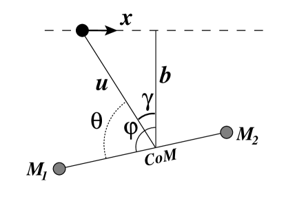
Figure 1.— Geometry of the lensing system. The black dot shows the projection of the source location onto the lens plane. The trajectory of the source in the lens plane is given by the dashed line. Note that we refer to the vertical line connecting the center of mass of the binary lens and the point of closest approach of the source as a CoM-b-axis.

Since general relativity is a nonlinear theory, the light curve produced by a binary lens is more complicated than a simple superposition of two amplification functions and cannot be described by an analytical formula. However, we can calculate the amplification value numerically as a function of source position in the lens plane (Schneider & Weiss, 1986; Witt, 1990). The result depends only on $\alpha$ and $q$. Given $b$ and $v$, we can calculate the trajectory of the source projection in the plane of the binary lens and construct the resulting light curve.

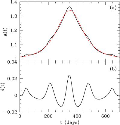
Figure 2.— (a) The black solid line shows a sample theoretical light curve with $b=1.0$ produced by our standard binary lensing system (see Section 4) rotating in retrograde direction. The dashed red line shows the least-$\chi^{2}$ fit single-lens light curve $A_{\rm SL}(t)$. (b) The residual light curve, defined as $\delta(t)=A(t)-A_{\rm SL}(t)$, clearly shows the effects of lens binarity. The oscillatory pattern contains information about the orbital motion of the lens.

Fig. 2(a) shows a sample light curve produced by our standard binary lens system which consists of two $0.5M_{\odot}$ stars (i.e. $M=1M_{\odot}$, $q=1$) in a circular orbit with $a=1\rm AU$. The lens-source system is set up (described in detail in Section 4) so that $\alpha=0.25$ and the timescale ratio is $\mathcal{R}=0.31$, representative of the $R\lesssim 1$ regime we are interested in. Over-plotted as a dashed red line is the best-fit single-lens light curve (Eq. 5). The overall shapes of the two light curves are very similar, which is not surprising for a binary with a fairly low value of $\alpha=0.25$. However, subtracting the single-lens fit from the binary light curve reveals a clear oscillatory pattern in the residuals, as shown in Fig. 2(b).

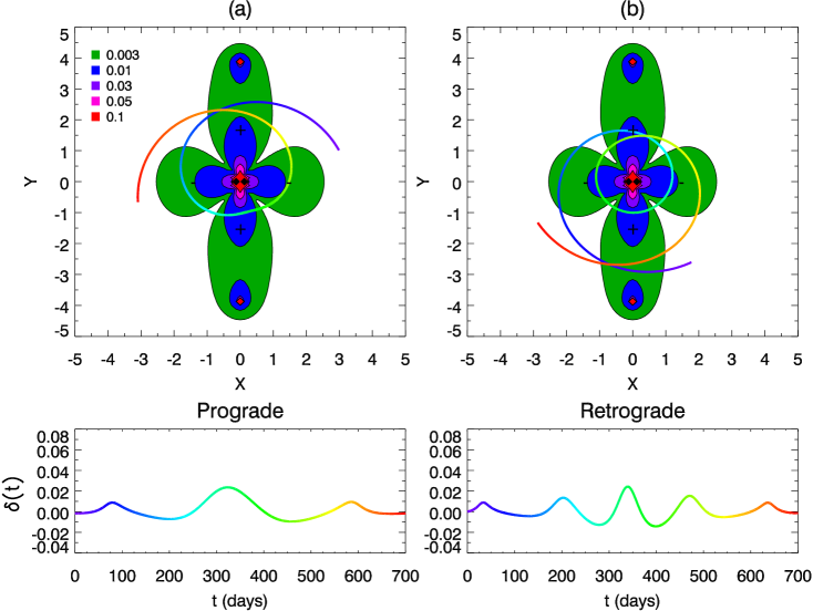
Figure 3.— Both panels show the contour plot of the absolute residual magnification function, $|\delta(x,y)|=|A(x,y)-A_{\rm SL}(x,y)|$, produced by the standard system (described in Section 4). The contour map is centered on the center of mass of the binary lens and the axes are in units of $R_{\rm E}$. The two binary components are located on the $x$-axis at $x=\pm\alpha/2=\pm 0.125$, indicated by the black dots. The horizontal elongated petals correspond to negative residuals and vertical petals correspond to positive residuals. The legend in panel (a) specifies the minimum values of $|\delta(x,y)|$ that correspond to different contour colors. As the source moves past the lens, its trajectory in the lens plane spirals in and out, producing the oscillatory residual pattern seen in the lower panels. Note that the colors of the trajectories and the residual curves are matched. Panel (a) shows the trajectory of the source with $b=1.0$ for the prograde binary lens, while panel (b) corresponds to the retrograde case (the light curve is identical to the one shown in Fig. 2).

To understand the relationship between this periodic pattern in the residuals and the orbital motion of the lens, it is instructive to examine the trajectory of the source in the lensing plane. In Fig. 3 we show this trajectory superimposed onto the contour plot of the absolute value of the residual magnification $|\delta(x,y)|=|A(x,y)-A_{\rm SL}(x,y)|$. Here $x$ and $y$ are coordinates in the lens frame, scaled to $R_{\rm E}$. The residual contours exhibit a nearly-symmetrical four-lobe shape. Note that the longer lobes (lined up with the y-axis) correspond to positive $\delta(x,y)$ values , while the shorter ones have $\delta(x,y)<0$. For face-on circular orbits $\alpha$ is time-independent and the amplification map is static. In the co-moving and co-rotating frame of the lens, the source appears to spiral in as it moves towards the point of closest approach and spiral out as it moves away from the lens. If the source were stationary, one full rotation of the binary lens would result in two full oscillations of the residual light curve. Thus, the periodicity of the residual signal is related to the orbital period of the binary lens by $T\sim T_{\rm orb}/2.$ Note that the relation is not exact due to the modification caused by relative transverse motion between the source and the lens.

To get a quantitative understanding of the interplay between source motion and binary rotation, we need to derive an equation for the time evolution of angle $\theta$, as shown in Fig. 1. Assuming that the source moves with velocity $v$ in the lens plane, its distance to the CoM-b-axis, scaled to $R_{\rm E}$, takes the form

$$x=\frac{t-t_{0}}{t_{\rm E}}.$$ (6)

The angle from the CoM-b-axis to the source is then given by

$$\gamma(t)=-\arctan\frac{x}{b}=-\arctan\frac{t-t_{0}}{bt_{\rm E}}$$ (7)

as shown in the geometry of the lensing system (Fig. 1). Notice that $\gamma(t)>0$ when $t<t_{0}$ and $\gamma(t)<0$ when $t>t_{0}.$ The phase angle from CoM-b-axis to the axis of the binary system is

$$\varphi(t)=\varphi_{0}\mp\omega_{orb}t,$$ (8)

where $\omega_{\rm orb}=\frac{2\pi}{T_{\rm orb}}$ is defined as the orbital frequency of the binary lens and “$-$” sign is adopted for prograde motion while “$+$” sign corresponds to retrograde motion. Finally, the angle between the source position and the axis of the binary is then

$$\theta(t) =\varphi(t)-\gamma(t)$$

$$=\phi_{0}\mp\omega_{\rm orb}t+\arctan\frac{t-t_{0}}{bt_{\rm E}}.$$ (9)

The distance from the source to the center of mass in the lens plane, $u(t)$ is given by Eq. (4). Note that the position of the source in the co-rotating lens plane is simply

$$x(t)=-u(t)\cos\theta(t),\qquad y(t)=u(t)\sin\theta(t).$$ (10)

A natural consequence of Eq. (9) is that the angular velocity of the source in the lens plane, $d{\theta}/dt$, is smaller for a prograde system than that for a retrograde system. This effect manifests itself clearly in the apparent period of residual signals shown in Fig. 3, which compares the trajectories of the source for a prograde and retrograde system with otherwise identical physical parameters. The retrograde residual light curve shows much faster oscillations because it has a larger value of $d{\theta}/dt$.

3. Timing Analysis

We now address the question of how to extract the information about the orbital periodicity of the binary lens from the observed microlensing light curves. We start by generating a theoretical binary light curve, add noise to simulate real survey data, subtract the dominant single-lens signal, perform spectral analysis on the the residuals, and examine the accuracy of the inferred orbital period.

3.1. Modeling the Observations

We can generate a theoretical light curve of arbitrary duration. To approximate realistic observing conditions, we take the photometric uncertainty to be $1\%$ for most of our calculations. (We discuss the results for high-precision photometry in Section 6.) At $u=3$, Eq. (5) gives $A_{\rm SL}\sim 1.01$, and so the overall amplification level is marginally distinguishable from random noise fluctuation. Based on this, we define the span of each lensing event to be from $3t_{\rm E}$ before the time of closest approach to $3t_{\rm E}$ after the closest approach. For all of our light curves we assume a fairly conservative average sampling interval of $\Delta t=2\;{\rm days}$. With this average rate, we sample the theoretical light curve at random times $\{t_{j}\}$ and add random Gaussian noise with mean 0 and standard deviation $0.01$ to each data point.

Finally, we fit Eq. (5) to our simulated light curve, both to obtain the residual light curve $\delta(t)$ as well as to determine our best-guess values for $b,t_{0},t_{\rm E}$, which are necessary for the subsequent timing analysis. We found that the fitting procedure works much better after smoothing out the sharp features, if any, produced by caustic crossings.

3.2. Modified Lomb-Scargle Analysis

Once we have the residual light curve we are ready to perform spectral analysis to extract the underlying periodicity of the binary. We base our period extraction method on the classical LS periodogram analysis (Scargle, 1982), a modification of the Fourier transform designed for unevenly sampled data that has the advantage of time-translation invariance.

Figure 4.— Periodogram of the light curve shown in Fig. 2. Panel (a) shows the results produced by the modified LS analysis. The highest-power peak corresponds to a period of 362 days, which is very close to the actual orbital period of the binary shown with a dashed line. Panel (b) displays the results of the standard LS periodogram analysis (here the power spectrum for negative period values is simply a mirror image of the positive part). The best-fit period of 266 days is clearly very different from either $T_{\rm orb}$ or $T_{\rm orb}/2$ shown by dashed lines.

For time series $\{\delta(t_{j})\}$ with $N$ data points, the LS periodogram as a function of frequency $\omega$ is defined as

$$P(\omega)=\frac{1}{2}\left[\frac{\left(\sum_{j=1}^{N}\delta(t_{j})C_{j}\right)^{2}}{\sum_{j=1}^{N}C_{j}^{2}}+\frac{\left(\sum_{j=1}^{N}\delta(t_{j})S_{j}\right)^{2}}{\sum_{j=1}^{N}S_{j}^{2}}\right]$$ (11)

where $C_{j}$ and $S_{j}$ are given by

$$C_{j}=\cos(\omega(t_{j}-\tau)),$$ (12)

$$S_{j}=\sin(\omega(t_{j}-\tau)),$$ (13)

and $\tau$ is defined as

$$\tau=\frac{1}{2\omega}\tan^{-1}\left[\frac{\displaystyle\sum_{j=1}^{N}\sin 2\omega t_{j}}{\displaystyle\sum_{j=1}^{N}\cos 2\omega t_{j}}\right]$$ (14)

Unsurprisingly, the unmodified LS periodogram analysis does not generally yield the correct binary period, since the frequency of the observed oscillatory signal, $\omega$, is affected by the relative source-lens motion (see Fig. 3) and is therefore not equal to the the binary orbital frequency, $\omega_{\rm orb}$. Figure 4(b) shows the LS power spectrum for a microlensing light curve with $b=0.4$ generated by our standard lensing system. The peak power corresponds to a period of 266 days, which is very different from both the true orbital period of the system, $T_{\rm orb}=372.5$ days, as well as $T_{\rm orb}/2$ (which we expect to come closer to reflecting the true variability timescale of the lensing signal due to the bi-fold symmetry of the magnification map produced by this binary, as illustrated by Fig. 3).

In Section 2 we argued that the progress of the lensing event is governed by the time evolution of angle $\theta$, defined by Eq. (9), which takes into account both binary rotation and source motion. Thus, we propose to modify the oscillating coefficients $C_{j}$ and $S_{j}$, essentially replacing $\omega t_{j}$ with $\theta(t_{j})$:

$$C_{j}=\cos[2\{\omega_{\rm orb}(t_{j}-\tau)-\gamma(t_{j})\}],$$ (15)

$$S_{j}=\sin[2\{\omega_{\rm orb}(t_{j}-\tau)-\gamma(t_{j})\}].$$ (16)

We dropped the $\varphi_{0}$ term in Eq. (9) since it simply produces a time translation of the signal without affecting the results of the LS analysis. The extra factor of 2 originates from the fact that the binary magnification pattern repeats itself twice over one binary revolution, and so the period directly observed in the data would be roughly half of the actual binary period, as we already pointed out above. Note that the definition of $\tau$ remains the same apart from replacing $\omega$ with $\omega_{\rm orb}$ in Eq. (14). Finally, the approximate values of $b$, $t_{0}$ and $t_{\rm E}$ necessary for evaluating $\gamma$ were obtained when fitting Eq. (5) to the original light curve.

Unlike the standard LS periodogram analysis for which only positive $\omega$ values have meaning, $\omega_{\rm orb}$ can have either sign. Following the sign convention in Eq. (9), when interpreting the results of the modified periodogram, $\omega_{\rm orb}<0$ corresponds to prograde systems while $\omega_{\rm orb}>0$ corresponds to retrograde systems.

Fig. 4 illustrates the difference between the results of the standard (panel (b)) and modified (panel (a)) periodogram analyses. Our new method produces a sharp power peak corresponding to the period $T=2\pi/\omega_{\rm orb}=362$ days, within 3% of the actual binary period. In addition, a positive period value correctly identifies the lens as a retrograde binary.

3.3. False Alarm Probability

The final issue we need to address is how to determine the minimum power level, $P_{\rm cut}$, such that any peak with a power above $P_{\rm cut}$ is unlikely to be produced by chance. Scargle (1982) derived a formula relating the false alarm probability $p_{\rm f}$ and $P_{\rm cut}$:

$$P_{\rm cut}=-\ln[1-(1-p_{f})^{1/N_{\omega}}],$$ (17)

where $N_{\omega}$ is the number of independent frequencies searched. For $p_{f}\ll 1$, we can approximate Eq. (17) as

$$P_{\rm cut}\approx\ln(N_{\omega}/p_{f})=\ln(N_{\omega})+\ln(1/p_{f}).$$ (18)

For a given value of $p_{f}$, $P_{\rm cut}$ depends only on $N_{\omega}$. There is no clear consensus in the literature on how to calculate $N_{\omega}$ for a given set of data, since the precise answer depends on the sampling method (Gilliland & Fisher, 1985; Baliunas et al., 1985; Horne & Baliunas, 1986). However, it is clear that $N_{\omega}$ must be on the order of the number of data points, $N$. We can thus rewrite Eq. (18) as

$$P_{\rm cut}-\ln(N)=\ln(N_{\omega}/N)+\ln(1/p_{f}),$$ (19)

and determine the term $\ln{N_{\omega}/N}$ empirically, using the same sampling scheme as we do for our light curves.

Figure 5.— Distribution of $P_{\rm max}-\ln(N)$ values for 5000 Gaussian random noise time series. The probability of detecting a spurious peak with a power $P>6+\ln(N)$ is less than 0.36%.

In order to do this, we simulated 5000 time series, randomly sampling pure Gaussian noise with 0 mean and $\sigma=1$. Each time series consisted of $N$ data points, with $N$ randomly chosen between 10 and 1000 using a uniform distribution in log space. We then applied the standard LS analysis to each time series by searching through frequencies from $2\pi$ to $N\pi$, and examined the distribution of $P_{\rm max}-\ln(N)$ values, where $P_{\rm max}$ is the power corresponding to the highest peak in each time series. We found that $P_{\rm max}-\ln(N)$ tended to increase as we increased $N_{\omega}$ but above $N_{\omega}=16N$ the distributions remained virtually unchanged. This worst case scenario is shown in Fig. 5. Based on this simulation, if we choose $P_{\rm cut}=6+\ln(N)$ as our significance criterion, then only 18 out of 5000 time series register $P_{\rm max}$ above this threshold. This corresponds to the false alarm probability of $18/5000=0.0036$, which compares well to $p_{f}=0.0025$, which we get from Eq. (18) if we set $N_{\omega}=N$. We adopted $P_{\rm cut}=\ln(N)+6$ as our detection threshold, i.e. only the peaks with power exceeding $P_{\rm cut}$ were treated as real detections.

4. The standard system

Having established our method for timing analysis, we first test it for what we call our standard binary lensing system. It consists of two $0.5M_{\sun}$ stars separated by a distance of $2a=2\,{\rm AU}$. We would expect this type of binary system to be fairly common since $0.5M_{\sun}$ stars lie near the peak of the IMF. We take the source to be near the Galactic Center at a distance of 8 kpc and set the lens at 4 kpc. For the relative transverse velocity, we adopt the value $v=60$ km/s. For these parameters, the ratio of the binary separation to the Einstein radius is $\alpha=0.25$ and the timescale ratio is ${\cal R}=0.31$. These are fairly conservative choices. On the one hand, $\alpha$ is low enough that the signatures of binarity will not be very prominent, as demonstrated in Figs. 2 and 3 (see also the discussion in Di Stefano & Esin, 2014). In addition, a relatively low value of the timescale ratio puts this binary firmly in the regime where both the orbital motion and the transverse motion of the source will play important roles in the formation of the light curve, making it an ideal testing system for our timing analysis.

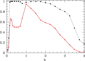
Figure 6.— The efficiency of our timing analysis for the standard system. The dashed black line shows the period detection rate, i.e. the fraction of the simulated light curves for which of a significant periodic signal is detected. The solid red line shows the correct period detection rate, i.e. the probability of extracting a significant orbital period that is within 10% of the true period of 372.5 days.

Our goal is to investigate the success of our proposed period extraction method for this system as a function of the impact parameter $b$. We want to determine how weak must be the overall amplification of a microlensing event must be for the periodicity in the light curve to no longer be detected. To this effect, we vary the value of $b$ from $0.05$ to $4.0$. Since low $b$ means stronger events and potentially more identified light curves in the existing lensing archives, we adopt a finer mesh for $b<0.8$ and a coarser mesh for larger values of $b$.

For each value of $b$ we generated 2000 light curves equally split between prograde and retrograde rotation directions. For each light curve, the initial phase angle $\varphi_{0}$ was randomly chosen from the interval $[0,2\pi]$. Each light curve was then analyzed using our method to determine (1) whether the power spectrum contains at least one peak with $P>P_{\rm cut}$, as defined in the previous section; and (2) whether the period corresponding to the peak with the highest power falls within 10% of the true orbital period of the lensing binary.

4.1. Period Detection Rates

The results are summarized in Fig. 6. As expected, the overall period detection rate (shown as a dotted black line) falls off with increasing $b$. This makes perfect sense because as the lensing event becomes weaker, the binarity signal becomes buried in the noise. Nevertheless, it is significant that most light curves are identified as periodic past $b=3$.

Of greater interest to us is the correct period detection rate (shown as a solid red line), i.e. the probability of extracting a significant orbital period that is reasonably close to the true period of the binary. For the purposes of this paper, we defined a detected period to be “reasonably close” if it lies within 10% of the true binary period of the lensing system (this also includes having the correct sign, i.e. distinguishing between prograde and retrograde rotation). This rate is falling faster with increasing $b$ than the overall detection rate, but even at $b=3$, we are still correctly identifying periods for 30% of all the light curves. Figure 7 shows the distribution of detected periods for light curves with $b=1.0$. It is clear that for most of these events we can use our method to determine the binary period to an accuracy of a few percent.

Figure 7.— Distribution of periods detected for $b=1.0$.

While the behavior of the detection rates for $b>1.0$ is easily understood, there are two peculiar features evident for the light curves with $b<1.0$. Firstly, for $b<0.2$ there is a steep drop in both detection rates. In addition, in the region $0,2<b<1.0$ there is a $\sim 50\%$ drop in the correct detection rate, while the overall detection rate remains near 100%. We investigate these in the remainder of this section.

4.2. High-frequency Signal in Low-$b$ Events

To diagnose the precipitous drop in the detection rates for $b<0.2$, we examine the trajectory and the corresponding residual light curve curves of an event with $b=0.1$ (see Fig. 8).

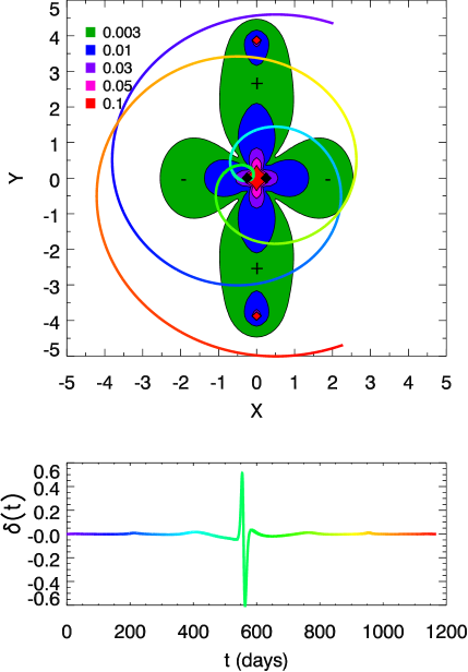
Figure 8.— Source trajectory and the corresponding residual light curve for a prograde standard system with $b=0.1$.

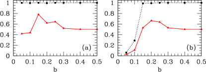
Figure 9.— Comparison of the detection rates with (panel [a]) and without (panel [b]) removing the high magnification ($A\geq 5$) portion of the light curves. The dotted black and solid red curves are defined as in Fig. 6.

The problem arises because the overall shape of the residual curve (lower panel of Fig. 8) shows a single strong high-frequency oscillation near the peak of the microlensing event. By relating the residual curve to the trajectory (upper panel of Fig. 8), we can see that it is due to the crossing of the red region between the two binary companions. Because of its relatively large amplitude, this high-frequency feature dominates our timing analysis and no significant period is detected in the data since it is never repeated .

A simple way of dealing with this issue is to simply remove the high-frequency part of the light curve so that the global low-frequency signal is given more weight in the timing analysis. To determine which part of the light curve to remove, we estimated the average radius of the red region to be $\sim 0.2R_{\rm E}$, and removed the corresponding portion of the light curve, i.e. the region with the overall magnification higher than $A_{\rm SL}(0.2)\approx 5$, where $A_{\rm SL}$ is given by Eq. (5). The detection rates with and without this modification to the timing analysis are shown in Fig. 9. Cutting out high magnification points appears to be highly effective; it restores the period detection rate to near 100% and raises the correct detection rate to at worst $50\%$ (Fig. 9(a)). Our investigation of other systems (Section 5) showed that his high-frequency signal contamination during close-approach events appears to be an universal problem. Thus, any results we show from this point on include this step in the timing analysis.

4.3. Prograde–Retrograde Period Confusion

To investigate the drop in the correct detection rate in the region $0.2<b<1.0$, we examined the statistics for prograde and retrograde systems separately. Fig. 10 demonstrates that this effect is mainly due to the prograde systems.

Next we examined the statistically significant though incorrect periods detected for the prograde light curves. It turns out that for many of these events the highest peak in the periodograms corresponds to a longer retrograde period $\sim+500$ days instead of the correct prograde period of $-372.5$ days, The correct period is also detected, but at a slightly lower power than the retrograde period. A periodogram of such a prograde light curve is shown in Fig. 11.

This confusion originates when subtracting the fitted single-lens light curve. Even a slight discrepancy between the actual and fitted values for $b$, $t_{\rm E}$ and $t_{0}$ introduces an extra bump near the peak of the light curve. This extra feature causes the prograde residual light curves to be mistaken for a retrograde one because the introduction of the extra peak in the prograde case will mimic the effect of higher frequency oscillations characteristic of retrograde light curves. In Fig. 12 we plot the probability that one of the two highest-power peaks lies within 10% of the correct period (dashed blue line), in addition to the two detection rates we have been discussing so far. This new detection rate shows that indeed most of the missing periods for low-$b$ light curves appear in the timing analysis as second-highest-power peaks. Interestingly, the detection rate of periods for higher $b$ light curves also significantly improves if we are willing to settle for two possible answers for the binary period.

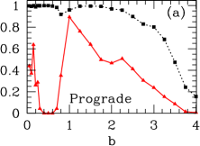
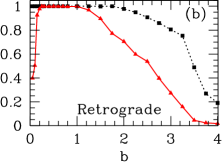
Figure 10.— Detection efficiency for the standard system for light curves with prograde (panel (a)) and retrograde (panel (b)) rotation.

Figure 11.— Periodogram of a prograde standard system with $b=0.4$. The highest peak corresponds to a longer retrograde period of $+491$ days while the true prograde period of $-372.5$ days has a lower power. The dashed line shows the location of the true system period.

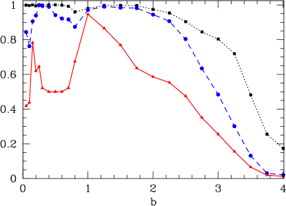
Figure 12.— Detection efficiency in standard system. The blue line represents the probability of either one of the highest peak and second highest peak lie in within 10% of the correct period of the system.

It turns out that this confusion between prograde and retrograde rotation is specific to our standard system rather than universal to binary lensing systems. In most of the other example systems that we discuss in Section 5, this issue hardly arises, except for one that is most similar to the standard binary, i.e. the probability of the highest peak being the correct period (red curve in Figure 13) is the same as one of the highest two peaks being the correct period (blue curve in Figure 13) for systems other than the standard and unequal.

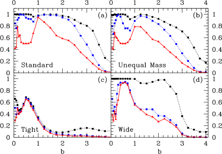
Figure 13.— Period detection rates for four systems summarized in Table 1.

5. Other example systems

We now examine the efficiency of our timing analysis technique for four other example lensing systems. For all of them we take $D_{\rm l}$ and $D_{\rm s}$ to be the same as for our standard binary. The rest of their physical parameters are summarized in Table 1 and the resulting period detection rates are plotted in Fig. 13. Note that panel (a) shows the results for our standard system for ease of comparison.

5.1. Unequal Mass Binary

This binary system is essentially equivalent to the standard binary lens system we discussed in the previous section except the masses of the two companions are $\frac{1}{3}M_{\sun}$ and $\frac{2}{3}M_{\sun}$, respectively. The effect of having $q\neq 1$ is the change in the shape of the residual amplification map; as illustrated in Fig. 14, the spatial asymmetry of mass distribution about the $y$-axis leads to the tilting of the “petals” in the residual pattern. As the source follows its spiraling trajectory in the lens plane, this asymmetry will certainly affect the spacing of the peaks, as illustrated in the light curves shown in the lower panels in Fig. 14, and can complicate the process of extracting the orbital period. However, it is encouraging that the detection efficiency for this system, shown in Fig. 13(b), is only marginally different than for the standard equal-mass binary (Fig. 13[a]). In fact, the overall shapes of the detection rates for the two cases are essentially identical when $b<1$. At larger values of $b$, for which the asymmetry is more pronounced, the unequal-mass system shows slightly lower detection rates, but the drop does not exceed 5-10%.

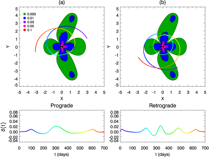
Figure 14.— Magnification map for the unequal-mass binary system. Since the two masses are not the same, the magnification map is not symmetrical with respect to the y-axis. Also plotted are the source trajectories with $b=1.0$ for both prograde (panel (a)) and retrograde (panel (b)) binary rotation directions, as well as the corresponding residual light curves.

5.2. Tight Binary

This system differs from the standard case only in its smaller binary separation. With $\alpha=0.15$, the characteristic binarity features in the residual light curves have very low amplitudes (see e.g. Di Stefano & Esin, 2014). On the other hand, smaller binary separation also means smaller orbital period. As a result, the timescale ratio is more than twice as large for this system as for our standard case, so the periodicity is easier to detect even in shorter duration light curves.

System	$M/M_{\odot}$	$q$	$T_{\rm orb}$ (day)	$v$ (km/s)	$\alpha$	${\cal R}$
Standard	1	1	372.54	60	0.25	0.3135
Unequal	1	0.5	372.54	60	0.25	0.3135
Tight	1	1	172.76	60	0.15	0.676
Wide	1	1	634.73	60	0.36	0.184

Table 1Summary of relevant parameters for the four example systems.

Looking at the detection rates shown in Fig. 13(c), it is clear that our results are dominated by the decrease in $\alpha$, the parameter which determines the amplitude of the features in the residual light curves. At best, we can detect periodicity in $\sim 60\%$ of all light curves and the probability of detection drops nearly to zero for $b>1.5$. However, because of the relatively high value of ${\cal R}$, when a period is detected the chances of it being correct are very high. The only exceptions are light curves with $b<0.1$, where the correct detection rate drops to about half of the total rate, just like it does for the standard system. We show in Section 6 that the detection rates for this system are very sensitive to the photometric precision of the data; with smaller noise the detectability can become very high (see Fig. 15(c)).

5.3. Wide Binary

We now consider the effect of having a larger binary separation while keeping all the other parameters the same. With $\alpha=0.36$, this lensing system will produce light curves characterized by much more pronounced deviations from the single-lens form. However, larger $a$ implies longer $T_{\rm orb}$ and therefore smaller ${\cal R}$, making period detection more difficult.

The results for the detection rates are shown in Fig. 13(d). In contrast to the small-separation system discussed in the section above, the overall detection rate for the wide binary light curves shows only a moderate decrease compared to the standard case. However, the correct detection rate drops significantly in the regime where $b\gtrsim 1$, reaching a maximum of $50\%$ near $b=1.0$ and dropping off to zero for $b>3$.

If we investigate the prograde and retrograde light curves separately, we can see that the gap between the two detection rates in the $b\gtrsim 1$ regime is caused predominantly by the prograde systems. In fact, taken by themselves, prograde light curves have the correct detection rate close to zero. The reason for this is simple. At ${\cal R}=0.184$ this binary straddles the boundary of detectability since its orbital period is slightly longer than the length of the microlensing event. In prograde binaries the effective period of the residuals is larger than $T_{\rm orb}$, so detection becomes virtually impossible. For retrograde binaries, the effective period is smaller than $T_{\rm orb}$ and can therefore be still detected. The correct detection rate in the regime $b<1$ is less affected since the magnification map has more features near the center of the mass of the binary lens and thus effectively produce more periodic signals in the light curves, which eases the correct detection of the period.

6. Low Noise Detection Rates

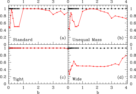
Figure 15.— Period detection rates for our four systems with 0.001% photometric uncertainties. The dashed black line shows the period detection rate and the solid red line shows the correct period detection rate as defined in Fig. 6.

While monitoring observations from the ground are unlikely to have photometric errors smaller than $\sim 1\%$, space-based missions, such as Kepler, TESS, and WFIRST, can do roughly 1000 times better (Koch et al., 2010; Ricker et al., 2014). It is highly likely that multiple microlensing events will occur in the field of those space-based telescopes over the lifetime of the mission, so it is worthwhile to consider how our period detection method would fare for data with photometric precision on the order of $0.001\%$. To that end, we have computed the period detection rates for our four systems in this low noise limit. Since high precision photometry would allow us to detect much smaller deviations, we expanded the length of our simulated light curves to $14t_{\rm E}$, instead of $6t_{\rm E}$ we adopted for higher noise levels.

Fig. 15 shows our new detection rates for the four systems. It is clear that the main effect of increasing photometric precision is a significant increase in detection rates, especially at high $b$. This result makes perfect sense: at large $b$, the overall light curve amplification as well as deviations from the point-lens form become small enough as to be non-detectable from the ground, but perfectly discernible from space.

Note that the overall rate of period detection now remains flat at essentially 100% all the way beyond $b=4$. Examining retrograde and prograde light curves separately, we again find that most of the gap between the overall and correct detection rates is attributable to prograde rotation.

The systems affected the most by the change in noise levels are the tight and wide binaries. The results for the former are particularly striking; where before we could detect at most $60\%$ of the periods, we now can detect the correct period for any light curve. The main reason for this improvement is again entirely due to the fact that very small amplitude signal can now be clearly detected. The value of $\alpha$ for this system places the binary features in the microlensing light curves at the edge of detectability with 1% errorbars, but this is not the case with improved precision.

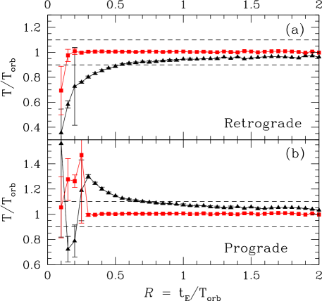
Figure 16.— Ratio of the detected to actual orbital periods of the binary lens as a function of ${\cal R}$ for LS (black triangles) and modified LS (red squares) periodogram methods. The results for the former were divided by a factor of 2 to compensate for the symmetry of the amplification pattern. Top and bottom panels show the results for retrograde and prograde light curves, respectively.

For the wide binary, the periods for prograde light curves were largely not detectable with higher noise levels since the length of the event was simply too long compared with the orbital period of the lens. Improved sensitivity allows us to follow the event for a much longer time, effectively decreasing the minimum value of ${\cal R}$ for which the periods can be reliably detected.

While the minimum value of ${\cal R}$ for which our timing analysis can be applied is set by the photometric precision of the data, we can place a firmer limit on the upper value of ${\cal R}$ for which our method is important. Clearly, when ${\cal R}\gg 1$, the lens-source relative motion becomes irrelevant and standard LS analysis should yield the correct period (up to a factor of 2) for such a binary lens.To see when the standard LS results begin to deviate significantly from the actual orbital period, we analyze, using both our modified LS and the standard LS methods, a series of light curves all with $b=1$, produced by lensing binaries with ${\cal R}$ spanning the range between $0.1$ and $2$. The other parameters of the lens binaries are the same as for our standard system with the exception of $a$, which was adjusted to vary $T_{\rm orb}$ and therefore ${\cal R}$. Fig. 16 compares the ratio of detected orbital period to the true orbital period of the binary $T/T_{\rm orb}$ using our modified LS method (red curve) and the standard LS method (black curve) as a function of ${\cal R}$.

We see that our proposed timing analysis method is very successful in extracting the correct orbital periods for the entire range of timescale ratios above the minimum set by the length of the light curves, while the standard LS periodogram algorithm clearly begins to fail (i.e. the detected period differs from the actual value by more than $10\%$) when ${\cal R}\lesssim 0.8$.

7. Discussion and Conclusions

When the Einstein crossing time is comparable to the orbital period of a binary lens, microlensing light curves display quasi-periodic features which can be used to determine $T_{\rm orb}$. In the limit when ${\cal R}\gtrsim 1$, the standard LS periodogram analysis can be used to find the period. However, in this paper we focus on the regime with ${\cal R}\lesssim 1$ when the variability timescale in observed light curves is set by a combination of binary rotation and relative source-lens motion. We have shown that this regime includes specific systems with orbital periods in the range from months to years. For such light curves the standard periodogram yields incorrect periods (see Fig. 4). Nucita et al. (2014) have noticed the same issue that the relative source-lens motion affects the periodic signals in binary microlensing light curves and thus prevents the correct orbital periodic extraction via the standard LS analysis. They proposed to circumvent the problem by removing the central part of the light curve and demonstrated its success on a few light curves. In this paper, we proposed a modification to the standard LS timing analysis method designed to compensate for the source motion and extract the correct orbital period. We tested our new timing analysis method on simulated light curves at two different noise levels for four different binary lens systems and calculated period detection rates for a wide range of impact parameter values averaged over random initial phase angles. The results are very encouraging. As long as the orbital period is detectable (i.e. not longer than the length of the simulated light curve) our proposed method finds and identifies it correctly in a large fraction of cases.

We find that the period detection rates are determined primarily by the photometric precision and three interdependent parameters, $\alpha$, ${\cal R}$ and $b$. Perhaps unsurprisingly, the photometric precision is the most important. It determines the minimum value of $\alpha$ for which binarity of the lens is detectable (Di Stefano & Esin, 2014) and sets the maximum value of $b$ for which a microlensing event is distinguishable from the noise. It also essentially sets the maximum practical length for a light curve which in turn determines the maximum detectable orbital period and therefore places a lower limit on ${\cal R}$.

We consider two levels of photometric uncertainty: 1%, characteristic of ground-based data, and 0.001%, relevant for dedicated space missions such as Kepler. In the first case, the reasonable event duration is $6t_{\rm E}$ (beyond this, the wings disappear into the noise) and, correspondingly, the detection rate drops off for ${\cal R}\lesssim 1/6$, as illustrated in Fig. 16 and well as by our results for the wide binary lens in Section 5.3. High-precision photometry allows us to significantly expand the parameter space for which the orbital periods can be reliably detected with our method.

We note that in our study, we model the light curves by treating the lensed star as a point source. This is well motivated by the fact that, for all the systems we considered in this paper, the angular size of a typical source star with radius $\sim 1R_{\odot}$ is only $\sim 0.06\%$ of the Einstein radius of the binary lens, negligible compared to any of the feature size in the magnification map. Under certain circumstances, e.g. when the source is a giant star located very close to the lens, finite-source effect can become important, reducing the amplitude and broadening the features in the residual curve. However, Penny et al. (2011a) showed that even in such extreme cases, the finite-source effect only affects a small portion of the binary features in the light curve. More importantly, since the finite-source effect does not significantly alter the timing of the periodic features, the result of the timing analysis shall not be affected, as long as the softened features are still detectable above the noise level.

As a proof-of-concept for our modified LS analysis, the results we discuss in this paper are based on the analysis of light curves produced by binary lenses in face-on circular orbits. We are now in the process of extending our calculations to include elliptical and inclined orbits. In these more complex situations, the projected binary separation, and with it the shape of the lensing magnification pattern, will vary with time during the microlensing event. This effect will certainly affect the spacing of the features in the residual light curves, possibly affecting the extraction of the orbital period. Our preliminary results indicate that the orbital period should still be detectable in a large fraction of light curves, but the full report will be the subject of a follow-up paper (M. Vick et al, in preparation).

Finally, we want to point out that in its present form, our timing analysis method works best for binary lenses with $q$ not very different from unity. It is predicated on the assumption that the oscillatory features repeat twice per orbit. The fact that period detectability does not change much from $q=1.0$ to $q=0.5$ (Fig. 13[a] and [b]) shows that some asymmetry in the magnification pattern can be easily tolerated. We tested lower values of $q$ for the unequal-mass system and found that the detectability decreases by a factor $\sim 2$ for $q=0.25$ and drops below $20\%$ for $q=0.1$. It is clear that in the planetary regime (i.e., when $q\ll 1$) a factor of 2 in Eqs. (15) and (16) does not apply, since the magnification pattern is no longer even remotely symmetrical (Di Stefano, 2012). Fortunately, such systems produce visibly different light curve morphologies characterized by very spiky rather than sinusoidal features (see Di Stefano & Esin, 2014, for some examples of light curves produced by low-$q$ binary lenses), and so can be flagged. We are now working on ways to extend our method to such low-$q$ systems.

References

- Albrow et al. (2000) Albrow, M. D., Beaulieu, J.-P., Caldwell, J. A. R., et al. 2000, ApJ, 534, 894
- Alcock et al. (1997) Alcock, C., Allen, W. H., Allsman, R. A., et al. 1997, ApJ, 491, 436
- Alcock et al. (2000) Alcock, C., Allsman, R. A., Alves, D., et al. 2000, ApJ, 541, 270
- An et al. (2002) An, J. H., Albrow, M. D., Beaulieu, J.-P., et al. 2002, ApJ, 572, 521
- Aubourg et al. (1993) Aubourg, E., Bareyre, P., Bréhin, S., et al. 1993, Nature, 365, 623
- Baliunas et al. (1985) Baliunas, S. L., Horne, J. H., Porter, A., et al. 1985, ApJ, 294, 310
- Di Stefano (2012) Di Stefano, R. 2012, ApJ, 752, 105
- Di Stefano & Esin (2014) Di Stefano, R., & Esin, A. 2014, ArXiv e-prints, arXiv:1412.7675
- Di Stefano & Mao (1996) Di Stefano, R., & Mao, S. 1996, ApJ, 457, 93
- Di Stefano & Perna (1997) Di Stefano, R., & Perna, R. 1997, ApJ, 488, 55
- Dominik (1998) Dominik, M. 1998, A&A, 329, 361
- Gilliland & Fisher (1985) Gilliland, R. L., & Fisher, R. 1985, PASP, 97, 285
- Henderson et al. (2014) Henderson, C. B., Gaudi, B. S., Han, C., et al. 2014, ApJ, 794, 52
- Horne & Baliunas (1986) Horne, J. H., & Baliunas, S. L. 1986, ApJ, 302, 757
- Hwang et al. (2010) Hwang, K.-H., Udalski, A., Han, C., et al. 2010, ApJ, 723, 797
- Jaroszyñski et al. (2010) Jaroszyñski, M., Skowron, J., Udalski, A., et al. 2010, Acta Astronomica, 60, 197
- Jaroszynski et al. (2004) Jaroszynski, M., Udalski, A., Kubiak, M., et al. 2004, Acta Astronomica, 54, 103
- Jaroszynski et al. (2005) —. 2005, Acta Astronomica, 55, 159
- Koch et al. (2010) Koch, D. G., Borucki, W. J., Basri, G., et al. 2010, ApJ, 713, L79
- Mao & Di Stefano (1995) Mao, S., & Di Stefano, R. 1995, ApJ, 440, 22
- Mao & Paczynski (1991) Mao, S., & Paczynski, B. 1991, ApJ, 374, L37
- Nucita et al. (2014) Nucita, A. A., Giordano, M., De Paolis, F., & Ingrosso, G. 2014, MNRAS, 438, 2466
- Paczynski (1986) Paczynski, B. 1986, ApJ, 304, 1
- Park et al. (2013) Park, H., Udalski, A., Han, C., et al. 2013, ApJ, 778, 134
- Penny et al. (2011a) Penny, M. T., Kerins, E., & Mao, S. 2011a, MNRAS, 417, 2216
- Penny et al. (2011b) Penny, M. T., Mao, S., & Kerins, E. 2011b, MNRAS, 412, 607
- Ricker et al. (2014) Ricker, G. R., Winn, J. N., Vanderspek, R., et al. 2014, in Society of Photo-Optical Instrumentation Engineers (SPIE) Conference Series, Vol. 9143, Society of Photo-Optical Instrumentation Engineers (SPIE) Conference Series, 20
- Ryu et al. (2010) Ryu, Y.-H., Han, C., Hwang, K.-H., et al. 2010, ApJ, 723, 81
- Sajadian (2014) Sajadian, S. 2014, MNRAS, 439, 3007
- Scargle (1982) Scargle, J. D. 1982, ApJ, 263, 835
- Schneider & Weiss (1986) Schneider, P., & Weiss, A. 1986, A&A, 164, 237
- Shvartzvald et al. (2014) Shvartzvald, Y., Maoz, D., Kaspi, S., et al. 2014, MNRAS, 439, 604
- Udalski et al. (1993) Udalski, A., Szymanski, M., Kaluzny, J., et al. 1993, Acta Astronomica, 43, 289
- Witt (1990) Witt, H. J. 1990, A&A, 236, 311
- Yock (1998) Yock, P. C. M. 1998, in Frontiers Science Series 23: Black Holes and High Energy Astrophysics, ed. H. Sato & N. Sugiyama, 375