Combining weak lensing tomography and spectroscopic redshift surveys

Abstract

Redshift space distortion (RSD) is a powerful way of measuring the growth of structure and testing General Relativity, but it is limited by cosmic variance and the degeneracy between galaxy bias $b$ and the growth rate factor $f$. The cross-correlation of lensing shear with the galaxy density field can in principle measure $b$ in a manner free from cosmic variance limits, breaking the $f-b$ degeneracy and allowing inference of the matter power spectrum from the galaxy survey. We analyze the growth constraints from a realistic tomographic weak lensing photo-$z$ survey combined with a spectroscopic galaxy redshift survey over the same sky area. For sky coverage $f_{\rm sky}=0.5$, analysis of the transverse modes measures $b$ to 2–3% accuracy per $\Delta z=0.1$ bin at $z<1$ when $\sim 10$ galaxies arcmin^-2 are measured in the lensing survey and all halos with $M>M_{\rm min}=10^{13}h^{-1}M_{\odot}$ have spectra. For the gravitational growth parameter parameter $\gamma$ ($f=\Omega_{m}^{\gamma})$, combining the lensing information with RSD analysis of non-transverse modes yields accuracy $\sigma(\gamma)\approx 0.01$. Adding lensing information to the RSD survey improves $\sigma(\gamma)$ by an amount equivalent to a $3\times$ ($10\times$) increase in RSD survey area when the spectroscopic survey extends down to halo mass $10^{13.5}$ ($10^{14}$) $h^{-1}M_{\odot}$. We also find that the $\sigma(\gamma)$ of overlapping surveys is equivalent to that of surveys 1.5–2$\times$ larger if they are separated on the sky. This gain is greatest when the spectroscopic mass threshold is $10^{13}$–$10^{14}h^{-1}M_{\odot}$, similar to LRG surveys. The gain of overlapping surveys is reduced for very deep or very shallow spectroscopic surveys, but any practical surveys are more powerful when overlapped than when separated. The gain of overlapped surveys is larger in the case when the primordial power spectrum normalization is uncertain by $>0.5\%$.

1 Introduction

Measurement of the linear growth of structure of the Universe is essential in that the growth history reflects the nature of dark energy and the underlying gravity model (e.g. Yamamoto et al., 2010), i.e. whether dark energy is a cosmological constant, or is evolving with time, or if General Relativity (GR) is the correct gravity model that governs the evolution of the Universe. In the linear regime of GR, the growth of perturbations is scale independent. It can be parameterized as the linear growth function $G$, with $P(z)=G^{2}(z)P_{\rm CMB}$, where $P(z)$ and $P_{\rm CMB}$ are the matter density power spectra at redshift $z$ and at the epoch of recombination, respectively. $G(z)$ carries information about the amount of dark energy and dark matter. The growth rate factor $f\equiv\frac{\partial\ln G}{\partial\ln a}$, with $a$ being the scale factor, is another quantify of interest: $f$ can be well approximated as $f=\Omega_{m}^{\gamma}$, with $\gamma$ in a narrow range near 0.55, for a wide variety of dark-energy models in General Relativity (Peebles, 1980; Lahav et al., 1991; Linder & Cahn, 2007). A precise measure of $\gamma$ therefore enables one to distinguish GR from alternative gravity models. In a braneworld type of modified gravity, for example, $\gamma$ is different from $\gamma_{\rm GR}$ by more than $20\%$ (Linder & Cahn, 2007).

Precise measurements of $G$ and $f$ constrain dark energy and gravity, and Redshift Space Distortion (RSD) has been shown to be a powerful approach to perform this measurement (e.g. Kaiser, 1987; Cole et al., 1994; Hamilton et al., 2000; Peacock et al., 2001; Scoccimarro, 2004; Guzzo et al., 2008; Cabré & Gaztañaga, 2009; Blake et al., 2011). This RSD measurement is, however, only precise in the linear regime. At late epochs of the Universe, the linear regime (of the velocity field in particular,) is confined to very large scales, $k\leq 0.1h^{-1}{\rm Mpc}^{-1}$. On these scales, the measurement is usually limited by sample variance, or cosmic variance—we do not have many independent perturbation modes for the measurement because of the finite survey volume observable in a given epoch.

Using multiple tracers of the density field, one can in principle evade sampling variance, and measure the linear growth of structure with unbounded accuracy (McDonald & Seljak, 2009; White et al., 2009; Gil-Marín et al., 2010; Bernstein & Cai, 2011). The great benefit of multiple tracers is not realized, however, if only the clustering of galaxies is measured because of the following: using RSD, one can only measure $\beta=f/b$ and the product $fG$. Without any prior knowledge of the galaxy bias, one can not constrain $f$ or $G$ independently. It has been shown by Bernstein & Cai (2011)[BC11] that prior knowledge on galaxy bias significantly improves the constraint on the growth of structure in the case of single survey redshift bin.

In principle, galaxy bias can be measured by cross-correlating weak gravitational lensing convergence with galaxy clustering (Pen, 2004). This bias measurement is free of sample variance in the sense that the bias errors from a survey of a fixed number of modes can be reduced without limit as the lensing measurement noise and galaxy shot noise are decreased. This enable us to use large-scale modes that are well in the linear regime for high-accuracy measurement (see BC11). Combining a weak lensing survey (using photometric redshifts for source galaxies) with a spectroscopic redshift survey of lens galaxies can serve this purpose perfectly: the bias of the spectroscopic galaxies is measured by cross-correlation with the lensing signal in transverse modes, while the RSD analysis of the spectroscopic sample is conducted using non-transverse modes over the same volume.

Current and future large surveys are making possible the combination of spectroscopic redshift-space and lensing maps over common volumes. For example, the footprints of the upcoming Dark Energy Survey (DES) may overlap with that of an extended Baryon Oscillation Spectroscopic Survey (BOSS) survey near the equator. The future Euclid space telescope (Laureijs et al., 2011) is designed to take spectra and images of galaxies at the same time.

In this work, we will explore the potential improvements in constraint of growth of structure and gravity from overlapping RSD and lensing surveys. This is an extension of BC11, where we consider the case of one single RSD redshift bin with an arbitrarily assigned prior on galaxy bias. In this work, we will consider the more realistic case of tomography using spectroscopic (RSD) and photometric (lensing) surveys covering common sky area, with both types of tracers divided into as many as 20 redshift bins. We will explore how well galaxy bias can be measured using the cross-correlation of galaxy shear and galaxy clustering in this realistic joint tomographic survey. The basic scheme is:

1. Conduct a galaxy redshift survey and a weak lensing (photo-$z$) survey over the same volume of the Universe. Split both galaxy samples into redshift bins.

2. Optimally weight galaxies in each bin of the redshift survey to produce a mass density estimator with minimal stochasticity (Hamaus et al., 2010; Cai et al., 2011). Measure the 2-point shear-shear (from the lensing survey), and density-density (from the spectroscopic survey) correlations and the shear-density cross correlations between all $z$-bins. Using these measurements of the covariance in transverse modes, constrain the bias $b$ of the spectroscopic galaxy density estimator and the mass power spectrum $P_{m}$ in each redshift bin.

3. In each $z$-bin, split galaxies from the redshift survey into different bias bins. Perform multiple-tracer RSD measurement (McDonald & Seljak, 2009; Bernstein & Cai, 2011) using the redshift-space density field of the binned galaxies. The $b$ and $P_{m}$ constraints derived from transverse modes in step 2 are incorporated to break the $f-b$ degeneracy inherent to RSD, so that separate constraints on $G$ and $f$ can be achieved. Throughout the paper, we will suppress the latin index denoting redshift in equations that involve only a single redshift bin, such as the RSD Fisher matrix. We use Greek indices for galaxy bias bins.

We use the Fisher matrix method to forecast growth constraints resulting from a model survey consisting of spectroscopic and lensing surveys covering a common $f_{\rm sky}=0.5$ of the sky, reaching the depth of $z=2$. We split both samples into 20 $z$-bins of width $\Delta z=0.1$. We employ the halo model for our survey model, assuming that each halo above mass $M_{\rm min}$ hosts one spectroscopic target galaxy. We set up our forecast methodology for lensing tomography in section 2 and for multi-tracer RSD in section 3. We summarize our numerical results in section 4, and conclude in section 5.

Unless noted otherwise, we assume a fiducial flat $\Lambda$CDM cosmology with the following parameters: $\Omega_{m}$=0.272, $\Omega_{\Lambda}=0.728$, $\Omega_{b}=0.0455$, $\sigma_{8}=0.807$, $n_{s}=0.961$, $H_{0}=70.2$. (Komatsu et al., 2011)

2 galaxy-shear cross-correlation

2.1 Weak lensing tomography

Weak gravitational lensing of background galaxies is a powerful way to measure the projected mass density of the foreground. It is free from galaxy bias and can be used to measure galaxy bias when cross-correlating with the galaxy density field. Source galaxies split into different tomographic bins enable us to probe the mass density at different epochs of the Universe.

For the $i$th $z$-bin of source galaxies, the observable of weak lensing is the distortion of those galaxy images, or cosmic shear, which is induced by foreground large-scale gravitational potential. From the cosmic shear one can infer the convergence $\kappa$, which is a weighted projection of the 3-D mass density of the foreground:

$$\kappa_{i}(\theta)=\frac{3H_{0}^{2}\Omega_{m}}{2c^{2}}\int^{\chi_{i}}_{0}\chi W_{i}(\chi)\frac{\delta(\chi\theta,\chi)}{a(\chi)}d\chi$$ (1)

where $\chi$ is the comoving radial distance, $a$ is the scale factor of the Universe, $\delta$ is the 3-D matter density contrast. The lensing weight function is

$$W_{i}(\chi)=\frac{1}{\bar{n}_{i}}\int^{\chi_{\rm H}}_{0}n_{i}(z)\frac{dz}{d\chi_{s}}\frac{\chi_{s}-\chi}{\chi_{s}}d\chi_{s},$$ (2)

where $\bar{n}_{i}$ is the number of galaxies in the $i$th redshift bin, distributed as $n_{i}(z)$. $\chi_{\rm H}$ is the horizon distance. We assume a total source redshift distribution of the form

$$n(z)=n_{0}z^{2}\exp(-z/z_{0}),$$ (3)

where $z_{0}=0.45$ is chosen to fit with the predicted Euclid survey’s median redshift, and $n_{0}$ is chosen such that $\int n(z)dz=N_{\rm lens}$, the total density of lens source galaxies per steradian. In section 4, we will examine results for a wide range of $N_{\rm lens}$.

The weak lensing signal is detectable only in statistics of large source-galaxy ensembles, e.g. via the two-point correlation function or its Fourier space counterpart, the shear power spectrum, or higher order correlation functions. Bernstein (2009) gives a framework for two-point analysis of weak lensing survey data. We follow the notation of Bernstein (2009) for the Fisher matrix from lensing tomography. We will work in the Fourier domain, and employ the Limber approximation (e.g. Limber, 1954; Kaiser, 1992; Hu, 2000; Verde et al., 2000; Cai et al., 2009), assuming that there is no correlation between $\delta$ in different redshift bins nor between different spherical harmonics. We also assume that within each redshift bin, $n_{i}(z)$ is a Dirac delta function at $z_{i}$, and that the projected mass fluctuations $\delta_{i}$ within bin $i$ can be treated as a single lens deflection screen at $z_{i}$. Under these assumptions, for a given spherical harmonic, the convergence of the $i$th source galaxy bin is just the weighted sum of the mass density of all the redshift bins in front of the $i$th bin ($i$ increases with redshift):

$$\kappa_{i}(l)=\sum_{k=1}^{i-1}A_{ik}\Delta\chi_{k}\delta_{k}(l)F_{k}+\epsilon_{i},$$ (4)

with $\langle\epsilon_{i}\epsilon_{j}\rangle=\delta^{K}_{ij}\sigma_{\epsilon}^{2}/n_{i}$ the variance of lensing shear noise. We take $\sigma_{\epsilon}=0.22$ throughout our calculation. $A_{ik}=\frac{D_{i}-D_{k}}{D_{i}}$, $D_{i}$ is the comoving angular diameter distance to redshift $z_{i}$, and $F_{k}=\frac{3}{2}H_{0}^{2}\Omega_{m}(1+z_{k})$.

2.2 Covariance matrix for lensing and galaxy density

When combining lensing tomography with a galaxy redshift survey over the same volume, we assume that the spectroscopic galaxies will be split into $z$ bins matching the source bins. A projected density estimator $\delta_{g}$ will be produced in each bin using some weighted combination of the spectroscopic galaxies. These projected density estimates are essentially the transverse modes of the RSD measurement in section 3. Each galaxy is given an optimal weight as described in section 2.4. The spectroscopic galaxies can have a different selection function from the lensing source galaxies. In cases where spectroscopic galaxies are not available (such as when we consider non-overlapping RSD and lensing surveys), we will assume that the $\delta_{g}$ measurement is made using galaxies with photometric redshift assignments from the lensing survey’s imaging data.

These measurements will be made for each mode transverse to the line of sight, indexed by spherical harmonic $l$:

1. $C^{\kappa\kappa}_{ij}(l)$—the (cross-) power spectrum of the lensing convergence at (and between) different redshift slices from the lensing survey.

2. $C^{gg}_{ij}(l)$— the power spectra at each redshift slice of the projected galaxy density estimator formed from the weighted spectroscopic galaxy survey (or photo-$z$ sample). We assume no correlation between densities of distinct redshift slices, following the Limber approximation and ignoring magnification biases and redshift mis-assignments, so ${\bf C}^{gg}$ is diagonal.

3. $C^{g\kappa}_{ij}(l)$—the shear-galaxy cross-spectra between different redshift slices. Galaxy density will only correlate with shear in the background, so ${\bf C}^{g\kappa}$ is a triangular matrix.

More specifically, the measurements can be expressed as:

$$C^{\kappa\kappa}_{ij}(l) = \sum_{k=1}^{min\{i,j\}-1}A_{ik}A_{jk}\Delta\chi_{k}P_{k}(l)F_{k}^{2}+\sigma_{\epsilon}^{2}\delta_{ij}/n_{i}$$

$$C^{gg}_{ij}(l) = D_{i}^{-2}\Delta\chi_{i}^{-1}P_{i}(l/D_{i})\bar{b}_{i}^{2}\delta_{ij}+{\cal N}_{i}(l)$$

$$C^{g\kappa}_{ij}(l) = A_{ji}D_{i}^{-1}P_{i}(l/D_{i})\bar{b}_{i}F_{i}\ |_{i<j}$$ (5)

where $n_{i}$ is the number density of lens source galaxies per steradian at the $i$th redshift bin; $P_{i}(k)=G_{i}^{2}P_{\rm CMB}(k)$ is the 3-D mass power spectrum at the $i$th redshift slice, with $G_{i}$ being the linear growth function at $z_{i}$; $l=k/D_{i}$ is the angular wavenumber; and $\bar{b}_{i}$ and ${\cal N}_{i}(l)$ are the scale-independent bias and stochastic noise power, respectively, of the weighted spectroscopic galaxy density estimator at $z_{i}$. Note that we ignore complications from intrinsic alignments of galaxies, photometric redshift errors, and other lensing measurement systematic errors.

The fiducial value of the noise term ${\cal N}_{i}(l)$ is taken from a fiducial stochasticity $E_{i}(l)$ of the galaxy density estimator: ${\cal N}_{i}^{\rm fid}(l)=E_{i}(l)^{2}D_{i}^{-2}\Delta\chi_{i}^{-1}P_{i}(l/D_{i})\bar{b}_{i}^{2}\delta_{ij}$. Our model for the fiducial $E_{i}(l)$ is taken from Cai et al. (2011) and described in section 2.4. The fiducial value of ${\cal N}_{i}(l)$ is taken from this model, but ${\cal N}_{i}(l)$ is still treated as an independent free parameter of $C^{gg}_{ii}(l)$, and will be marginalized over. Note that most analyses (including our own RSD Fisher matrix) assume that the stochastic power is known a priori to be given by the Poisson formula. We find in this lensing analysis that a strong prior knowledge of ${\cal N}$ can substantially influence the final growth constraints, so we adopt a weak conservative prior quantified below.

For each spherical harmonic $l$, the full covariance matrix for the lensing and density measurements is

$${\bf C}=\left[\begin{array}[]{cc}{\bf C^{\kappa\kappa}}&{\bf C^{g\kappa}}\\ {\bf(C^{g\kappa})^{T}}&{\bf C^{gg}}\end{array}\right],$$

which is a $40\times 40$ matrix for our 20 redshift slices $z_{i}={0.1,0.2...2.0}$.

2.3 Fisher matrix of the cross-correlation

The free parameters of the model for the lensing Fisher matrix are:

1. The amplitude of the mass power spectrum at different redshift $P_{i}(l/D_{i})$, which is in turn a function of only the linear growth function $G_{i}$ at redshift $z_{i}$, $P_{i}(l)=G_{i}^{2}P_{CMB}(l/D_{i})$. In practice we use the parameter $p_{i}=\ln P_{i}(l)=2\ln G_{i}+{\rm const}$.

2. The bias $\bar{b}_{i}$ of the weighted spectroscopic galaxy density. It is related to the biases $b_{i\alpha}$ of individual galaxy bins used in the RSD analysis by $\bar{b}_{i}=\sum_{\alpha}w_{i\alpha}b_{i\alpha},$ with the weights $w_{i\alpha}$ as assigned in Section 2.4. How galaxies are made into different bias bins is detailed in Section 3

3. The noise ${\cal N}_{i}(l)$ in the galaxy-galaxy clustering measurement in transverse modes.

We fix all parameters except for the 20 $P_{i}$, 20 $\bar{b}_{i}$ and 20 ${\cal N}_{i}$—note that this includes taking the cosmological distances $D_{i}$ as known. There are no lensing sources behind the highest redshift bin, so the last bias parameter is unconstrained. We therefore drop the rows and columns of the Fisher matrix for the $\bar{b},P,$ and ${\cal N}$ parameters of the highest redshift bin, leaving $57\times 57$ elements at each multipole $l$:

$${\bf F^{pq}_{Lens}}(l)=\frac{1}{2}{\rm Tr}\left[{\bf C}(l)^{-1}{\bf C}(l)_{,p}{\bf C}(l)^{-1}{\bf C}(l)_{,q}\right]$$ (6)

where $p,q\in\{P_{i},\bar{b}_{i},{\cal N}_{i}\}$. The above equation holds true because $<\kappa>=0$ for the whole sky. For the first bin, there is no constraint from lensing, so the first row and column of $C_{l}^{\kappa\kappa}$ are zero. We add priors on the ${\cal N}_{i}$ parameters to indicate uncertainties propotional to the fiducial values:

$$F^{{\cal N}{\cal N},prior}_{ij}(l)=\delta_{ij}\left(2{\cal N}_{i}^{\rm fid}\sqrt{\alpha N_{l}}\right)^{-2}.$$ (7)

$N_{l}$ is the number of $l$ bins that we use. This scaling produces a prior such that the mean ${\cal N}_{i}$ over all $l$ bins in known to accuracy $2\alpha{\cal N}_{i}^{\rm fid}$. We choose the very weak prior $\alpha=50$ for our calculation.

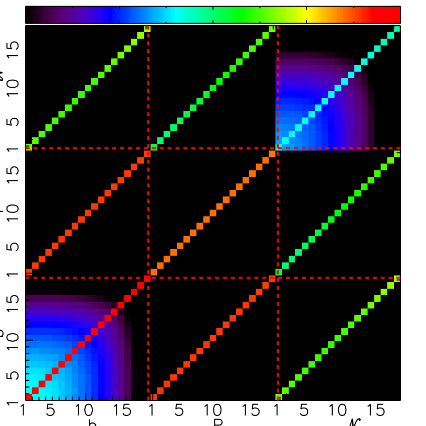
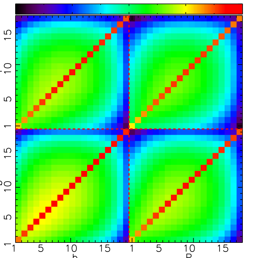
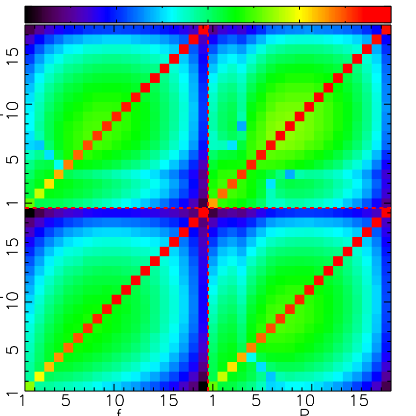
An example of the lensing Fisher matrix is shown in the left panel of Figure 1 for a single mode at $l=30$. We find the Fisher matrix is close to block-diagonal, i.e. $\bar{b}^{\prime}s$, $P^{\prime}s$ and ${\cal N}^{\prime}s$ at distinct $z$ are only weakly correlated. Lowering the fiducial stochasticity ${\cal N}_{i}$ makes the Fisher matrix more diagonal.

Figure 1: Examples of Fisher matrices for 20 redshift bins for weak lensing source density $N_{\rm lens}=10{\rm arcmin}^{-2}$ and spectrosopic survey depth $M_{\rm min}=10^{12}M_{\odot}$; each survey covers $f_{\rm sky}=0.5$. Left: Fisher matrix ${\bf F_{\rm Lens}}$ from joint lensing/galaxy measurements on transverse modes at $l=30$, with parameters for bias $\bar{b}$, mass power $P$, and galaxy stochastic power ${\cal N}$ at each $z$; Middle: ${\bf F_{\rm Lens}}$ for linear $\bar{b}$ and $P$ after marginalizing over all $\bar{b}$’s and $P$’s of non-linear modes, summing over all $l$, and marginalizing all ${\cal N}$’s; Right: Fisher matrix about $f$ and $P$ after summing ${\bf F_{\rm Lens}}+{\bf F_{\rm RSD}}$, after marginalizing over all biases. Each matrix block contains parameters from low $z$ in lower-left to high $z$ in upper right, as labeled, omitting the highest $z$ bin which is unconstrained. Fisher matrices use logarithms of each parameter so that fractional errors are represented. The fiducial value of stochastic powers ${\cal N}$ are estimated from halo mode described in section 2.4 and a weak prior is applied. Note that correlations between distinct redshifts are always quite weak.

2.4 Sources of noise in the lensing measurement

In the determination of the $\bar{b}_{i}$ using the cross-correlation of lensing and galaxy surveys, both the shear measurement noise and stochasticity between the tracer and the mass field serve as sources of error. We can rewrite Equation (4) as

$$\kappa_{i}(l) = \sum_{k=1}^{i-1}A_{ik}\Delta\chi_{k}F_{k}\left(\frac{\delta^{g}_{k}(l)}{\bar{b}_{k}}-e_{k}(l)\right)+\epsilon_{i},$$ (8)

$$= \sum_{k=1}^{i-1}A_{ik}\Delta\chi_{k}F_{k}\frac{\delta^{g}_{k}(l)}{\bar{b}_{k}}-s_{i}(l)+\epsilon_{i},$$ (9)

with the galaxy overdensity $\delta^{g}_{k}(l)$=$\bar{b}_{k}\delta_{k}(l)+e_{k}(l)$, where $e_{k}$ is the stochastic component. The lensing observable hence has two indistinguishable stochastic components that are not properly traced by the galaxies—its shear measurement noise $\epsilon_{i}$ plus the total convergence from the mass fluctuations $s_{i}(l)=\sum_{k=1}^{i-1}A_{ik}\Delta\chi_{k}F_{k}e_{k}(l)$. Together these degrade the constraint on the mean bias, and also affect the constraint on the mass power since $\bar{b}$ and $P$ are strongly correlated (see the Fisher matrix of $\bar{b}$ and $P$ at the middle panel of figure 1). We will investigate in Section 4.1 how the choices of lensing source density $N_{\rm lens}$ and spectroscopic depth $M_{\rm min}$, which set these two noise levels, affect the constraint on $\bar{b}$ and $P$, and further affect constraints on the growth.

Since the stochasticity of the galaxy density has been shown to be a limit for the precision of weak lensing constraints on the bias (e.g. Pen, 2004), we have incentive to reduce the stochasticity below the commonly assumed Poisson level. Sub-Poisson stochasticity has been demonstrated in $N$-body simulations, (e.g. Bonoli & Pen, 2009; Hamaus et al., 2010; Cai et al., 2011). Here we follow the method of Cai et al. (2011), hereafter CBS, for minimizing the stochasticity of a mass estimator from a weighted combination of halos.

The optimal weight $w_{\rm opt}$ of each halo is a function of its mass and of the minimum mass $M_{\rm min}$ of halo included in the survey. The resulting stochasticity between the weighted halo field and the mass field $E_{\rm opt}$. Explicit expressions from CBS for $w_{\rm opt}$ and $E_{\rm opt}$ are given in the Appendix. With this definition of $E_{\rm opt}$, the stochastic components of the galaxy density clustering can be written as $<e(l)e^{\prime}(l)>=E_{\rm opt}^{2}(l)/[1-E_{\rm opt}^{2}(l)]$. This expression is a function of redshift, but for simplicity, we drop the latin index denoting redshift here.

In this work, we use the CBS halo model description of $E_{\rm opt}$ to produce the fiducial value of stochastic power ${\cal N}_{i}(l)$. In principle, both $w_{\rm opt}$ and $E_{\rm opt}$ are functions of the Fourier wave number $k$, the minimal halo mass of the catalogue $M_{\rm min}$ and redshift $z$. However, since we find that $w_{\rm opt}$ depends very weakly on $k$ in the linear regime, we will just adopt the $w_{\rm opt}$ for $k=0.01h\,{\rm Mpc}^{-1}$ at each $M_{\rm min}$ and $z$. CBS shows how $E_{\rm opt}$ drops with $M_{\rm min}$; therefore, a deeper spectroscopic redshift survey targeting galaxies hosted by lower-mass halos leads to a higher-precision measure of the galaxy bias when cross-correlated with lensing.

In using the CBS model for our fiducial value of $E$, we are assuming that the host halo mass of each spectroscopic target is known by some means, and that the spectroscopic targets are complete to the limiting halo mass. This assumption might be somewhat strong but it is not impossible for a real survey. One can imagine using the relatively deep lensing image survey to resolve satellite galaxies that are hosted by each spectroscopic galaxy’s halo. The number of satellite galaxies could then be used to estimate the halo mass. We need a spectroscopic redshift of only the central galaxy of each halo.

When we are forecasting scenarios in which there is no overlapping spectroscopic survey for lensing data at a given $z$, we assume that photometric redshift maps can produce a $\delta_{g}$ density estimator with fiducial stochasticity $E_{i}=0.5$. Note that the bias $\bar{b}$ for the photo-$z$ population can not be used in this case to constrain the biases of the spectroscopic population because of different selection functions.

2.5 Summation over modes

In the lensing Fisher matrix, we marginalize over all noise parameters ${\cal N}_{i}$ to have $(19b^{\prime}s+19P^{\prime}s)^{2}$ left. We also marginalized over all those b’s and P’s of non-linear modes. In marginalizing over non-linear modes, we will retain more modes at high $z$, since for fixed $l$, the physical scale is larger at high $z$. Furthermore, non-linearity develops on smaller scales at higher redshift. Since accurate predictions of redshift distortions will likely be available only in the linear regime, we do not use non-linear modes in our measurements.

To separate linear and non-linear modes, we first assume that at $z=0.5$, the linear modes have $k<k^{0.5}_{\rm max}=0.1h\,{\rm Mpc}^{-1}$. We then compute the variance $\sigma^{2}(R^{0.5}_{\rm min},z=0.5)=\frac{1}{2\pi^{2}}\int k^{2}P(k)W^{2}(kR^{0.5}_{\rm min})dk$ smoothed by a spherical top-hat window function $W(x)=3[\sin(x)-x\cos(x)]/x^{3}$ with the radius $R^{0.5}_{\rm min}=2\pi/k^{0.5}_{\rm max}$. We choose the scale of $R^{z}_{\rm min}$ at all other redshifts so that $\sigma^{2}(R^{z}_{\rm min},z)=\sigma^{2}(R^{0.5}_{\rm min},z=0.5)$. We obtain $k^{z}_{\rm max}=2\pi/R^{z}_{\rm min}$, and $l_{\rm max}^{z}=k^{z}_{\rm max}D(z)$ for each z.

After marginalizing over non-linear $\bar{b}$’s and $P$’s at each $l$, we sum the Fisher matrices for linear-regime parameters over all modes with $l_{\rm min}<l<l_{\rm max}$, with $l_{\rm min}=10$ for all redshifts:

$${\bf F^{pq}_{Lens}}(l)=\sum_{l=10}^{l_{\rm max}}f_{sky}(2l+1){\bf F^{pq}_{Lens}}(l).$$ (10)

An example of the final lensing Fisher matrix is shown in the middle panel of Figure 1. While the constraints on $\bar{b}_{i}$ and $P_{j}$ are highly correlated for $i=j$ , the corrrelations among $\bar{b}$ and $P$ at distinct redshifts are very weak, and we can consider the experiment to give essentially independent results at every redshift bin.

3 Multi-tracer redshift space distortion

In this section, we review the basic idea of using redshift space distortion (RSD) to measure the growth of structure. This will be implemented in a spectroscopic survey. For each redshift shell, galaxies will be made into multiple bins of their parent halos’ masses. Our measurements will include the redshift space power spectra of each sub-sample, and the covariance of all those galaxy bins.

Each redshift shell of the spectroscopic survey will have an independent Fisher matrix.

In the linear regime, galaxy overdensity $\delta^{s}$ seen in redshift space will be boosted relative to the matter overdensity $\delta$ due to the large-scale inflow bulk motion of galaxies. The first-order large-scale peculiar velocity is related through the continuity equation to the linear growth rate factor $f\equiv\frac{\partial\ln G}{\partial\ln a}$. The redshift-space galaxy clustering therefore encodes information on the growth of structure. In Fourier space, Kaiser (1987) derives

$$\delta^{s}_{\alpha}({\bf k})=(b_{\alpha}+f\mu^{2})\delta({\bf k})+\epsilon_{\alpha},$$ (11)

with $\epsilon_{\alpha}$ the stochastic portion of the galaxy density with $\langle\epsilon_{\alpha}\delta\rangle=0$. For the RSD analysis we assume a diagonal stochasticity matrix, $\langle\epsilon_{\alpha}\epsilon_{\alpha}\rangle=\delta^{K}_{\alpha\beta}/n_{\alpha}$ i.e. noise in distinct galaxy bins is uncorrelated. $b_{\alpha}$ is the bias of the ${\alpha}$th galaxy bin, and $\mu$ is the cosine of the angle between the $k$ vector and the line of sight.

Following BC11, the covariance of the multi-tracer RSD measurement is:

$$C_{\alpha\beta}({\bf k}) = {\rm Cov}(\delta^{s}_{\alpha}({\bf k}),\delta^{s}_{\beta}({\bf k}))$$

$$= (b_{\alpha}+f\mu^{2})(b_{\beta}+f\mu^{2})G^{2}P_{CMB}({\bf k})+{\cal E}_{\alpha\beta},$$

$${\cal E}_{\alpha\beta} \equiv \langle\epsilon_{\alpha}\epsilon_{\beta}\rangle.$$ (13)

The free parameters in this measurement are: the biases $b_{\alpha}$ of the galaxy bins, assumed to be scale independent; the growth rate $f$, the linear mass power spectrum $P=G^{2}P_{\rm CMB}$, where $G$ is the linear growth function and $P_{\rm CMB}$ is the power spectrum at the epoch of recombination. For each mode at each redshift bin, we have the Fisher matrix (Tegmark et al., 1997) of RSD:

$${\bf F^{pq}_{RSD}}({\bf k})=\frac{1}{2}{\rm Tr}\left[{\bf C}({\bf k})^{-1}{\bf C}({\bf k})_{,p}{\bf C}({\bf k})^{-1}{\bf C}({\bf k})_{,q}\right]$$ (14)

where $p,q\in\{f,P,b_{1},b_{2}...b_{N_{b}}\}$. We assume that galaxies are binned by the mass of their parent halos, use three log mass bins for each decade of mass ($N_{b}=15$ mass bins for the case of $M_{\rm min}=10^{11}M_{\odot}$). The size of the Fisher matrix is $(N_{b}+2)\times(N_{b}+2)$. This multi-tracer RSD method improves the constraint of $fG$ by a factor of up to 6.4 compared to the standard RSD method, where all galaxies are placed in one single bias bin (BC11). Without any prior knowledge of galaxy bias, neither method can constrain $f$ or $G$ alone, only the product $fG$.

Nonlinear $k$ modes will not be used in our analysis, applying the criteria from section 2.5. We sum over modes within $k_{\rm min}<k<k^{z}_{\rm max}$, where $k_{\rm min}=l_{\rm min}D(z)$, to yield a total RSD Fisher matrix for our redshift bin:

$${\bf F^{pq}_{RSD}({\bf k})}=\frac{V}{(2\pi)^{3}}\sum_{\mu=-1}^{1}\Delta\mu\sum_{k=k_{\rm min}}^{k_{\rm max}}4\pi k^{2}{\bf F^{pq}_{RSD}}(k)\Delta k.$$ (15)

Here $V$ is the surveyed volume within the redshift bin under consideration. When integrating the RSD matrix over $\mu$, we are careful to remove a section around $\mu=0$ representing the number of transverse modes used in constructing ${\bf F_{\rm Lens}}$ for the same bin of redshift and $k=l/D$. This avoids double-counting the information in the transverse modes of the spectroscopic survey if we are analyzing overlapping RSD and lensing surveys. For non-overlapping surveys, we do not exclude the $\mu=0$ modes from the RSD information.

3.1 Combining RSD and lensing Fisher matrices

Note that the RSD Fisher matrix is degenerate in the $f$–$b$ direction. Combining RSD measurement with a lensing survey can break the degeneracy between $b$ and $f$, and hence yield a tighter constraint on $\gamma$. There may, however, be non-zero covariance between $b$ or $P$ values at different redshifts in the lensing measurement. So when combining the constraints from lensing with those from RSD, the parameters in each $z$ bin can not be treated independently. We will need to create a large joint Fisher matrix for biases, $f$, and $G$ at all redshifts, so we concatenate ${\bf F^{pq}_{RSD}}$ from all 19 redshifts into a single block-diagonal RSD matrix.

We have to convert the lensing and RSD Fisher matrices to encompass a common set of parameters, then sum them, being careful not to double-count information. The final Fisher matrix will contain entries for the $N_{b}$ bias values $b_{i\alpha}$, plus the growth and growth rate $G_{i}$ and $f_{i}$ at each of the 19 measurable redshift bins, giving a final dimension of $19\times(N_{b}+2)$. The matrix is nearly block-diagonal with isolated redshift blocks, because ${\bf F_{\rm RSD}}$ is completely decoupled between redshift bins, and ${\bf F_{\rm Lens}}$ is nearly so. We retain the full matrix, however, for completeness.

The lensing Fisher matrix elements for galaxy bias refer to the weighted mean bias $\bar{b}_{i}=\sum_{\alpha}w_{i\alpha}b_{i\alpha}$ for each redshift. We can convert the constraint on the weighted mean bias into a joint constraint on the individual bins’ biases using the known weights $w_{i\alpha}$ from the Appendix.

4 results

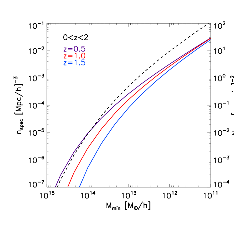
In this section, we compare the constraints on the growth of structure from having a lensing photo-$z$ survey, a spectroscopic redshift survey, and the combination of them. We will also investigate the case of having the two surveys over separate volumes. We will explore how the results may depend on the depth of the spectroscopic survey and the photo-$z$ survey. For the spec-$z$ sample, we usually label the survey depth as the minimal halo mass $M_{\rm min}$, since we assume that the spectroscopic targets are the central galaxies of all halos with $M>M_{\rm min}.$ Figure 2 plots the space density of targets vs $M_{\rm min}$ at a few nominal redshifts, plus the total projected sky density of targets vs $M_{\rm min}$. For example, $M_{\rm min}\sim 10^{12}h^{-1}M_{\odot}$ corresponds to galaxies of Milky Way size or larger, with a space density of $\sim 10^{-2.5}h^{3}{\rm Mpc}^{-3}$ and sky density $\sim 10\,{\rm arcmin}^{-2}$; having $M_{\rm min}\sim 10^{13}M_{\odot}$ is like a Luminous Red Galaxy (LRG) sample, with a space density of $\sim 10^{-3.5}h^{3}{\rm Mpc}^{-3}$ and sky density $\sim 1\,{\rm arcmin}^{-2}$; and $M_{\rm min}=10^{14}h^{-1}M_{\odot}$ is a rich cluster survey, with a space density of $\sim 10^{-5}h^{3}{\rm Mpc}^{-3}$ at $z<1$ and sky density $\sim 0.01\,{\rm arcmin}^{-2}$. Keep in mind that the survey targeting $M>M_{\rm min}$ generally yields the best possible cosmological constraints for a given target density.

Figure 2: Galaxy number density $n_{\rm spec}$ in the spectroscopic survey versus the minimum halo mass $M_{\rm min}$ at three different redshifts estimated from halo model. We assume one spectroscopic target per halo. Black dashed line shows the projected galaxy number density versus $M_{\rm min}$ at $0<z<2$.

We will assume that the primordial CMB power spectrum is known exactly, unless specified otherwise. We will show that for most cases, knowing $P_{\rm CMB}$ to $0.5\%$ gives about the same growth constraints as fixing it.

Figure 3: Lensing constraints on $\bar{b}$ and $G$ (dotted lines), RSD constraint on $fG$ (dashed lines) and lensing+RSD constraint on $f$ and $G$ (solid lines) in each redshift bin of width $\Delta z=0.1$ are plotted vs redshift, for the case of $N_{\rm lens}=10\,{\rm arcmin}^{-2}$. Left: $M_{\rm min}\sim 10^{13}M_{\odot}$ and Right: deeper spectroscopic survey, $M_{\rm min}\sim 10^{12}M_{\odot}$. As the depth of spectroscopic survey increase, the constraints on $\bar{b}$ and $G$ from the lensing-galaxy cross-correlation improves, because the stochasticity of the galaxy sample with respect to mass goes down when smaller halos are mapped. The constraint on $fG$ also improves with the spectroscopic survey depth. The joint constraint on $f$ and $G$ also improves with spectroscopic depth at high $z$ in particular. Adding lensing data to RSD splits the $fG$ constraint into separate $f$ and $G$ constraints, which are substantially more precise.

4.1 Lensing constraint on $\bar{b}$ and $G$

We first examine the constraints on $\bar{b}$ and $P$ at different $z$ bins from ${\bf F_{\rm Lens}}$, the joint analysis of lensing and galaxy density surveys in purely transverse modes. Assuming the primordial power spectrum $P_{\rm CMB}$ is known, measuring $P$ is the same as measuring the linear growth function $G$.

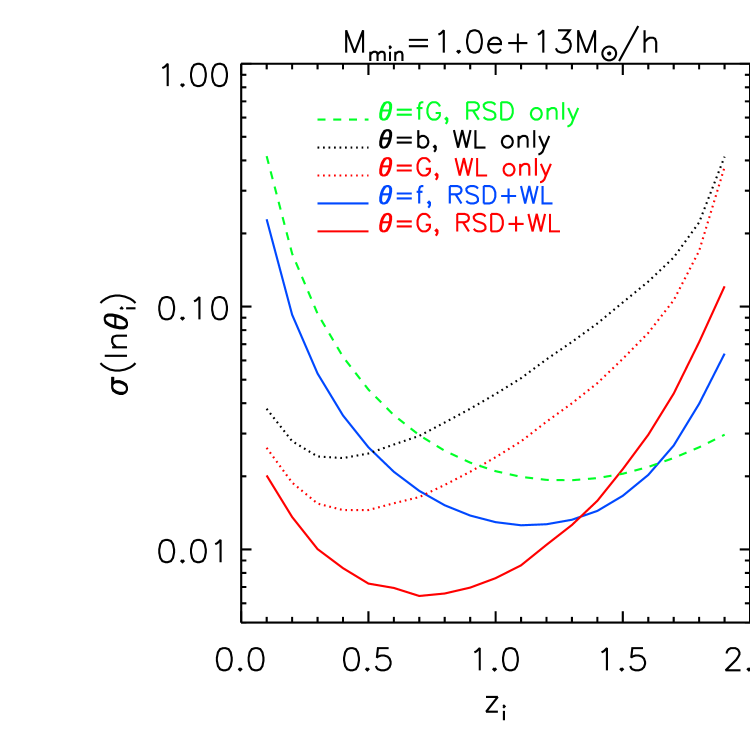
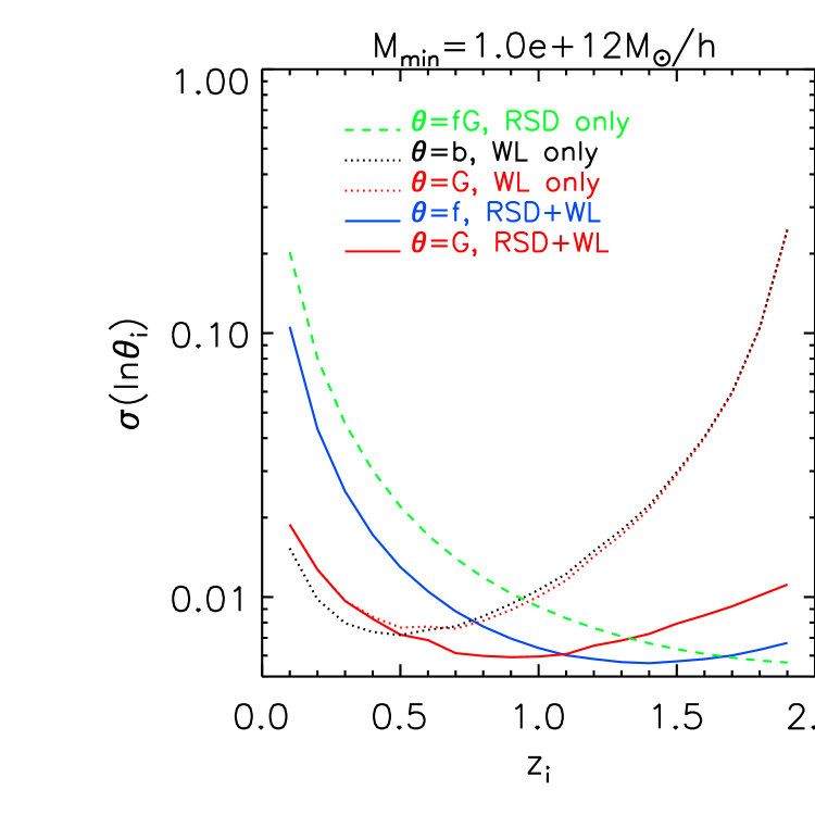
The dotted lines in Figure 3 plot the Fisher uncertainties in $\bar{b}_{i}$ and $G_{i}$ (the equivalent of $\sqrt{P_{i}}$) vs redshift $z_{i}$. Each plotted point gives errors after marginalization over all other parameters. We find the measurements of galaxy mean bias and $G$ reach percent-level accuracy over a large range of redshifts for $M_{\rm min}=10^{13}h^{-1}M_{\odot}$ (left panel), and sub-percent accuracy when galaxy stochasticity is lower with $M_{\rm min}=10^{12}h^{-1}M_{\odot}$ (right panel). The constraint is better at low redshift, easily understood since higher-redshift lenses have fewer background galaxies to lens and hence higher effective shape noise in the lensing measurement.

The number of available linear modes increases rapidly at higher $z$, which should in principle cause constraints to improve with redshift. While we see this behavior at $z<0.5$, the constraints become weaker at $z>0.5$, indicating that the increasing shape noise and galaxy stochasticity dominate the improving mode counts.

4.2 RSD constraint on $fG$

Having RSD measurement alone, one can measure the parameter $fG$ after marginalizing over $f/b$. The green dashed lines in Figure 3 show the constraint on $fG$ using the multi-tracer RSD method. We find $fG$ is better constrained at high $z$, opposite to the lensing constraints on $\bar{b}$ and $G$ shown in the previous subsection. The gain at high $z$ for $\sigma(fG)$ mainly comes from having more modes as the survey volume $dV/dz$ grows with redshift. When $M_{\rm min}$ is smaller (comparing the right-hand panel to the left), $\sigma(fG)$ also drops, as expected, since we have more galaxies with a broader range of biases.

BC11 show, and we confirm here, that there is little change in the cosmological constraints from the multi-tracer RSD analysis from allowing the shot noise level to be a free parameter instead of fixing the Poisson value.

4.3 Combined constraint on $f$ and $G$

The $\bar{b}$ and $G$ measurement from lensing-galaxy cross-correlation in transverse modes can be added to the RSD analysis in the 3-D spectroscopic redshift survey over the same volume. This will help to break the $f$–$b$ degeneracy existing in the case when RSD alone is available. Separate constraints on $f$ and $G$ are then achieved after marginalization over all the bias parameters, leaving 19 $f$’s and 19 $P$’s in the Fisher matrix. An example of ${\bf\tilde{F}^{f_{i}P_{j}}_{Lens+RSD}}$ is shown in the right hand panel of Figure 1. As expected, the $f-P$ Fisher matrix exhibits very little correlation between different redshifts.

The solid lines of Figure 3 plot example constraints on $f$ and $G$ vs $z$ after marginalizing over all other parameters. The redshift dependence of $\sigma(f)$ is similar to that of $\sigma(fG)$, and the combined constraint on $G$ improves significantly over the case when lensing alone is available. This improvement is more prominent at high $z$.

4.4 Constraint on gravity

Figure 4: Log of uncertainty $\sigma(\gamma)$ on growth parameter $\gamma$ as a function of spectroscopic survey limit $M_{\rm min}$ and lensing source density $N_{\rm lens}$. Color scale and contour levels are identical for all panels: Upper left: RSD measurement only; Upper right: lensing tomography only (including cross-correlation with photo-$z$ galaxy samples); Lower left: lensing survey $+$ galaxy redshift survey over the same volume at $0<z<2$, including cross-correlation between spectroscopic sample and lensing; Lower right: the same as lower-left panel, but the two surveys are not overlapping, so there is lensing cross-correlation with photo-$z$ galaxies but not the spectroscopic sample. Note that in this case, the total number of modes are more than the case shown at lower left, i.e. the transverse modes of the two surveys are now independent.

Figure 5: Left: the square of the ratios of $\sigma(\gamma)$ from RSD measurement versus that from lensing+RSD measurement. This is essentially showing how much larger a survey area the RSD measurement would need to achieve the same accuracy on $\gamma$ as when lensing information is added. Right: the same as the left but showing the ratio of lensing+RSD from separate volumes versus lensing+RSD over a common volume. The overlapping survey is most beneficial along a band with $M_{\rm min}\approx 10^{14}M_{\odot}$. For deeper spectroscopic surveys, the separate surveys are nearly equivalent to overlapping, because the lensing information is a weak addition whether or not overlapping. Likewise for very shallow spectroscopic surveys and deep lensing survey (upper left corner), the lensing information dominates and overlap of RSD is irrelevant.

Figure 6: Comparing $\sigma(\gamma)$ as a function of $M_{\rm min}$ from lensing measurement (dotted lines), RSD measurement (dashed lines) and RSD+Lensing (solid lines) with different priors on $P_{\rm CMB}$ in different colors. Left: the number density of galaxies in the lensing survey is $N_{\rm lens}=10\,{\rm arcmin}^{-2}$. Right: ultra-deep lensing survey wtih $N_{\rm lens}=100/,{\rm arcmin}^{-2}$. When $M_{\rm min}$ is large so the number density of halos in the galaxy redshift survey is small, constraints on $\gamma$ mainly come from lensing tomography. When the spectroscopic survey is deep, addition of lensing data does not improve the constraint on $\gamma$ substantially. If we had forecast a single-tracer RSD analysis instead of multi-tracer RSD, then the gain from adding lensing to a deep spectroscopic survey would be larger. Note that adding $0.5\%$ prior on $P_{\rm CMB}$ improves the constraint on $\gamma$ by a factor 2, and is close to the case of knowing $P_{\rm CMB}$ perfectly. The red stars indicate where RSD+Lensing is worse than lensing alone in the constraint of $\gamma$. This is because in the lensing alone case, we are using the projected galaxy-galaxy clustering from the lensing photo-$z$ sample. The stochasticity in this case can be lower than that of the spec-$z$ sample, when $M_{\rm min}$ is very large.

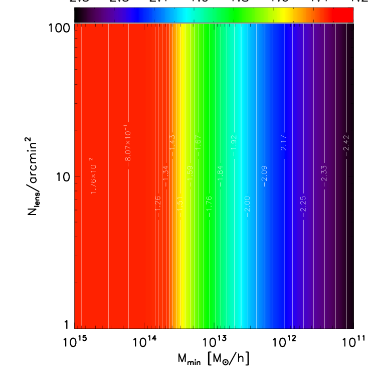
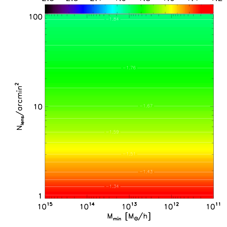
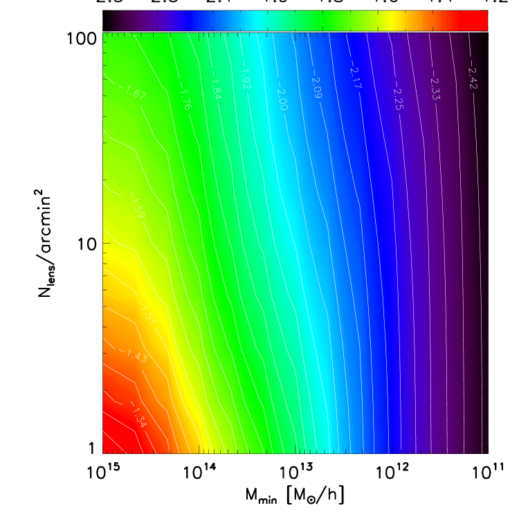
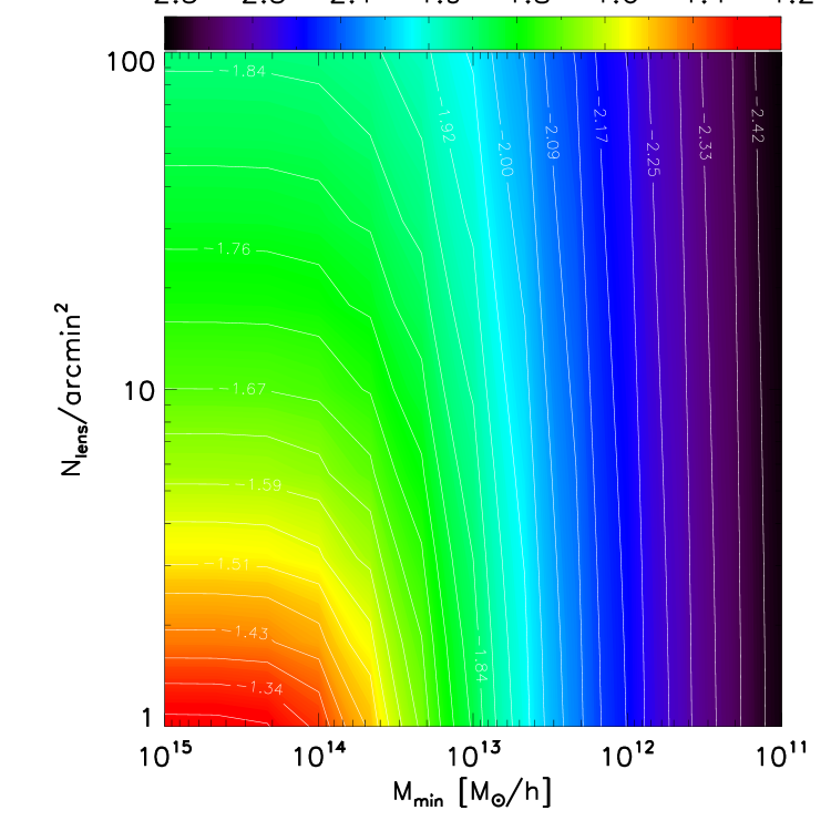
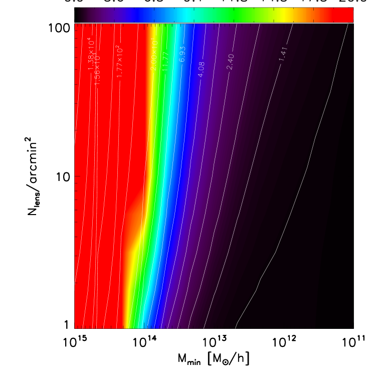
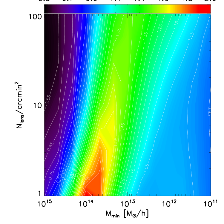
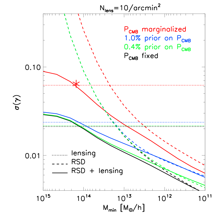
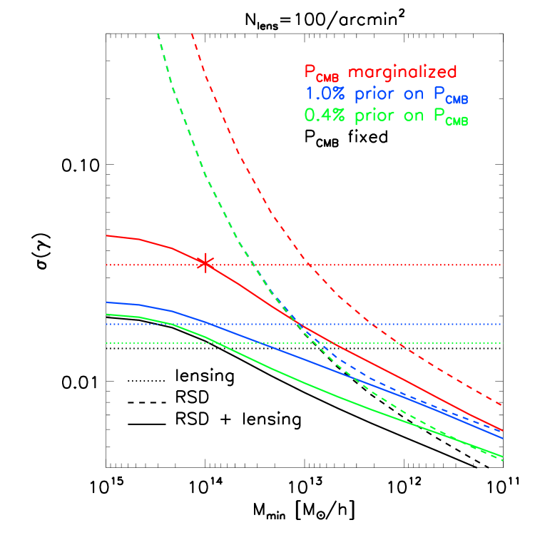
In the fiducial ${\rm\Lambda}$CDM cosmology, a change in $\gamma$ results in predictable changes in the growth history ($f$ & $G$). Therefore, constraints on growth can be translated into a constraint on $\gamma$. We present $\sigma(\gamma)$ as a function of $N_{\rm lens}$, the number density of a lensing survey, and $M_{\rm min}$, which is equivalent to the survey depth of a spectroscopic redshift survey. In Figure 4, we compare four different cases: having RSD alone (I) (top left), lensing alone (II) (top right), RSD plus lensing over the same volume (III) (bottom left) and RSD plus lensing in separate volume (IV) (bottom right). All results we show assume that the primordial CMB power spectrum is known, unless specified otherwise. Figure 6 plots $\sigma_{\gamma}$ vs $M_{\rm min}$ at two distinct $N_{\rm lens}$ values, for different strengths of prior knowledge of the amplitude of $P_{\rm CMB}$. Marginalization over the normalization of $P_{\rm CMB}$ leads to $\sigma_{\gamma}$ constraints about a factor 2 worse than knowing $P_{\rm CMB}$ exactly, but a prior with 0.5% accuracy on $P_{\rm CMB}$ recovers almost all of this loss.

4.4.1 (I) RSD alone

When using multi-tracer RSD from a spectroscopic redshift survey, the result strongly depends on the survey depth, or $M_{\rm min}$ (upper left plot of Figure 4 and dashed lines in Figures 6. By surveying halos with down to $M_{\rm min}\sim 10^{12}h^{-1}M_{\odot}$, RSD alone can already constrain $\gamma$ to $\sim 1\%$. The current GAMA survey reaches this survey depth (Robotham et al., 2011) up to $z\sim 0.5$, but one need to expand the survey to cover half of the sky in order to achieve this accuracy. As $M_{\rm min}$ increases, $\sigma(\gamma)$ increases rapidly—$\sigma(\gamma)\sim 2\%$ for $M_{\rm min}\sim 10^{13}h^{-1}M_{\odot}$ and $\sigma(\gamma)\sim 10\%$ for $M_{\rm min}\sim 10^{14}h^{-1}M_{\odot}$ (equivalent to galaxy number density of $10^{-6}$–$10^{-5}\,{\rm Mpc}^{-3}$).

Central LRGs are considered as good samples for RSD measurement, as they reside at the center of their host halos therefore should be free from the non-linear finger-of-God effect (Okumura & Jing, 2011; Hikage et al., 2011). They are hosted by halos with $M_{\rm min}>10^{13}h^{-1}M_{\odot}$ (e.g. Zheng et al., 2009). LRGs are, however, an incomplete sampling of halos near $10^{13}h^{-1}M_{\odot}$. Therefore, RSD with LRG samples may not be as powerful as the $M_{\rm min}=10^{13}h^{-1}M_{\odot}$ forecast here.

4.4.2 (II) lensing alone

When a lensing survey alone is available, we can still estimate the mass density in the transverse modes using photo-$z$ galaxies. In this case, the stochasticity between the galaxy density field and the mass field may be larger, so we conservatively assume $E_{\rm fid}=0.5$ and add a weak prior on the ${\cal N}$ term as we have discussed in section 2.3.

For this case of joint shear/density tomography without spectra, $\sigma(\gamma)$ varies by a factor of $\approx 5$ when $N_{\rm lens}$ varies from 1 to 100 (Figure 4, upper right). The upcoming DES is expected to have $N_{\rm lens}\sim 10\,{\rm arcmin}^{-2}$, which if scaled to $f_{\rm sky}=0.5$ constrains $\gamma$ down to $\approx 2\%$ (Figure 6, left). Future surveys like LSST or Euclid, attaining $N_{\rm lens}\sim 40\,{\rm arcmin}^{-2}$ in the most optimistic scenario, yield $\approx 1.25\times$ reduction in $\sigma_{\gamma}$.

Removing the CMB constraint on the amplitude of the primordial power spectrum may increase the error in $\gamma$ by a factor of 2.

4.4.3 (III) RSD + lensing (same volume)

Combining the two surveys will in general help to improve the constraint on $\gamma$. The $\sigma(\gamma)$ for the overlapping surveys is plotted in the lower left of Figure 4. The left-hand plot of Figure 5 quantifies the improvement from adding lensing to the spectroscopic survey as the inverse square of the improvement in $\sigma(\gamma)$, which is equivalent to asking what factor more survey area the RSD survey would require in order to match the improvement from the addition of lensing data. The amount of improvement depends on many factors.

When the spectroscopic redshift survey is very deep, i.e. $M_{\rm min}\sim 10^{12}h^{-1}M_{\odot}$, RSD alone can already measure $\gamma$ at sub-percent level, if combined with $0.5\%$ constraint on the primordial power spectrum from the CMB (Figure 6). The number density of halo redshifts in such a survey is $n_{spec}\sim 10^{-3}h^{3}\,{\rm Mpc}^{-3}$, requiring a total of $\sim 10^{8}$ redshifts over half of the sky. In this regime, the improvement in the constraint of $\gamma$ by adding lensing data is very minor, and changing the lensing survey depth will not affect the result. This is consistent with the result of BC11 (see their Figure 3).

Figure 3 displays dramatic gains in constraint of $f$ and $G$ at $z>1.2$ when $M_{\rm min}$ is reduced from $10^{13}$ to $10^{12}h^{-1}M_{\odot}$, yet only modest gains in $\sigma(\gamma)$ are seen in Figure 6 or on the left of Figure 5. This is because both the absolute values of $\partial P/\partial\gamma$ and $\partial f/\partial\gamma$ become smaller at high $z$, where $\Omega_{m}$ is close to 1, so measures of $f$ and $P$ at $z>1$ are less valuable in constraining gravity under this parameterization.

When only halos with $M>10^{13}h^{-1}M_{\odot}$ are targeted in the spectroscopy survey, the benefit of combining with a lensing survey becomes more prominent: equivalent to a factor of 2 to 3 increase in survey volume at $M_{\rm min}\sim 3\times 10^{13}h^{-1}M_{\odot}$, and more than $10\times$ when $M_{\rm min}\sim 10^{14}h^{-1}M_{\odot}$! (See left of Figure 5 and Figures 6.) However, even in this regime, lensing is never completely dominant in the range of $N_{\rm lens}$ we are considering, in the sense that Figure 4 shows that improving the spectroscopic survey depth is always substantially beneficial for measuring $\gamma$.

4.4.4 (IV) RSD + lensing (separate volume)

Here we compare the power of lensing and RSD surveys conducted over a shared $f_{\rm sky}=0.5$ to surveys that do not overlap, covering distinct volumes. Having two surveys in separate volumes has the advantage of having twice as many transverse modes as the case of overlapping survey volumes; is this advantage outweighed by knowing the bias of the spectroscopic survey galaxies through the overlapped lensing survey?

To forecast the $\gamma$ constraints from separate surveys, we make the following alterations to the Fisher methodology for the combined surveys: first, we construct ${\bf F_{\rm Lens}}$ under the assumption that photo-$z$ samples are being used for the galaxy density map ($\Rightarrow E_{\rm fid}=0.5$). Then we marginalize the $\bar{b}_{i}$ values in ${\bf F_{\rm Lens}}$ to leave constraints over only the $P_{i}$. For the RSD Fisher matrix, we marginalize over all the $b_{i\alpha}$ since no lensing constraints are available, leaving behind only a constraint on the product $fP$ at each redshift. We also allow the RSD analysis to use all transverse modes, since these are no longer redundant with those in the lensing survey. The lensing and RSD Fisher matrices can again be summed and projected onto a single $\sigma(\gamma)$, plotted in the lower right of Figure 4. We also plot, on the right-hand side of Figure 5, the effective area gain of the overlapping survey relative to separate surveys. Note that this area “gain” could be as low as 0.5, i.e. a loss, since the combined survey does cover only half the volume of the separate ones.

We find that having two surveys over the same volume is better than having them separated except for extremely deep lensing or spectroscopic surveys. The improvement is equivalent to a factor of 1.5 to 2 in survey volume when $10^{13}h^{-1}M_{\odot}<M_{\rm min}<10^{14}h^{-1}M_{\odot}$, but very minor when the spectroscopic redshift survey gets deeper. This is true when the primordial CMB power spectrum is known to better than $0.5\%$. If we do not employ any CMB constraint and marginalize over $P_{\rm CMB}$, then the $\gamma$ constraint will be degraded for each case, but the gain of having overlapping survey volume versus separate volume is larger, e.g. a factor of 3–4 in the regime when $M_{\rm min}$ is large. The area gain factor is $\approx 1.5$ even when the spec-$z$ is deep. Therefore, having a weak CMB prior makes the idea of combining two surveys over the same volume more useful, while a strong CMB prior help to reduce $\sigma(\gamma)$ in both cases and narrows the difference between them.

Notice on the lower-right of Figure 4 that in the regime when $M_{\rm min}>10^{13.5}h^{-1}M_{\odot}$ (shallow spectroscopic redshift survey), the constraint from lensing measurements is dominant and the depth of the non-overlapping spectroscopic survey becomes irrelevant.

In summary, combining two surveys help most, relative to separate surveys, when the spectroscopic redshift survey is modestly sparse, $M_{\rm min}\approx 10^{13.5}h^{-1}M_{\odot}$, in the range of LRG surveys. When the spectroscopic survey is deep ($M_{\rm min}<10^{13}h^{-1}M_{\odot}$), it dominates the error budget and it matters less whether the lensing survey overlaps or not. On the other hand, when the spectroscopic survey is very shallow ($M_{\rm min}>10^{14.5}h^{-1}M_{\odot}$), then even a modest lensing survey ($N_{\rm lens}>5\,{\rm arcmin}^{-2}$) dominates the information, and it matters less whether the spectroscopic survey is coincident. There is, however, no regime of feasible large-scale surveys for which the separate surveys constrain $\gamma$ better than overlapping surveys.

5 conclusion and discussion

We have shown from Fisher matrix forecast that the constraint on the growth of structure and gravity can be reduced percent-level or even sub-percent level by combining a spectroscopic redshift survey with a photo-$z$ weak lensing survey over the same volume. Whereas BC11 merely assumed that some measure of galaxy bias was available to add to RSD information, we verify here that a realistic tomographic weak lensing survey does in fact yield bias information sufficient to realize a substantial gain in accuracy on the growth parameter $\gamma$.

Following the suggestions of Pen (2004) we use the shear-galaxy cross-correlation to measure the galaxy bias in the transverse modes—a measurement which is free of sample variance—and apply it to the multi-tracer RSD analysis in a spectroscopic redshift survey (McDonald & Seljak, 2009; Bernstein & Cai, 2011). The combination of the two surveys make it possible to measure the linear growth function $G$ separately from its derivative $f=d\ln G/d\ln a$, whereas RSD alone can only measure the product $fG$.

The performance of multi-tracer RSD measurement depends on the spectroscopic survey depth, the range of galaxy biases in the sample, and the number of linear modes available. The performance of the shear$+$galaxy analysis on the transverse modes depends on: (1) the level of stochasticity between the galaxies and the projected mass, (2) the depth of the lensing survey, or shape noise. When combining two measurements together over the same volume, the results will depend on all those factors that affect each of the survey.

We have demonstrated that for the constraint of the $\gamma$ parameter, combining two surveys is better than having each of them alone, roughly a factor 1.5 improvement (in survey-area terms) in the regime of likely feasible surveys: source density $N_{\rm lens}\approx 10\,{\rm arcmin}^{-2}$ in the lensing survey, and galaxy surveys complete for halos in the cluster or small-group range $M_{\rm min}=10^{13}$–$10^{14}h^{-1}M_{\odot}$, similar to LRG surveys. For $M_{\rm min}>10^{13}h^{-1}M_{\odot}$, the lensing$+$RSD survey has constraints many times more powerful than the RSD survey alone. The $\gamma$ parameterization of growth predicts very little change at $z>1$; a different model for deviations from General Relativity could gain even more from the combination of lensing and RSD surveys.

Having prior constraints on the amplitude of the primordial power spectrum from the CMB is useful in general. Knowing $P_{\rm CMB}$ to $0.5\%$, easily within the statistical power of Planck, garners most of the $\approx 2\times$ gain in accuracy on $\gamma$ that is possible with perfect a priori knowledge of $P_{\rm CMB}$. If $P_{\rm CMB}$ is more poorly known, the gain of having overlapping surveys over the case of separate survey volume is increased.

During preparation of this paper, Gaztanaga et al. (2011) released very similar calculations of the benefit of coincident lensing and spectroscopic surveys. Their assumed survey configurations and free parameterizations differ substantially from ours, so direct quantitative comparison is not possible. In the particular case of constraints on $\gamma$, they find overlapping surveys reducing $\sigma(\gamma)$ by $\approx 2.4\times$ compared to seperated survey volumes, equivalent to a $6\times$ increase in survey area in the language of our Figure 5 where we find $\approx 1.5\times$ areal gain. This is qualitatively consistent with our conclusion, but the origin of the substantial quantitative difference is difficult to ascertain given the different assumptions about survey characteristics. Gaztanaga et al. (2011) also find substantial gains in accuracy of dark energy equation-of-state determination from overlapping surveys. Our analysis holds this fixed so we would not have detected these gains; we plan to broaden our analysis to the case of unknown distance-redshift relations in the near future.

We notice that bias measurement can in principle also be measured using the same spectroscopic sample from the galaxy bispectrum (Simpson et al., 2011). If the same accuracy of bias can be obtained in this method as using lensing, one can simply use one spectroscopic redshift survey to obtain the same measurement, which might be another attractive survey strategy since no lensing survey is needed. The lensing survey is, however, a straightforward measure of the galaxy bias, free of assumptions about perturbation theory, second-order bias, and other issues with the bispectrum.

Use of smaller-scale modes are attractive in the sense that one may gain many more modes from the same volume of survey. Growth test statistical accuracy improves rapidly with increasing $k_{\rm max}$. Non-linear effects in the density or velocity field and scale-dependent bias may, however, ruin the attempt to achieve percent-level constraint on parameters. Efforts have been made to improve RSD predictions for smaller-scale modes (Scoccimarro, 2004; Jennings et al., 2011; Hikage et al., 2011; Tang et al., 2011), e.g. $k_{\rm max}\sim 0.3$, though it is important that predictions be made for galaxies or halos rather than all mass particles in an $N$-body simulation (Jennings et al., 2011), e.g see Reid & White (2011) for modeling of halos. Better understanding of the non-linear biases of different tracers is required before one can confidently select the $k_{\rm max}$ that admits the most accurate growth constraints.

Appendix A optimal weighting and minimal stochasticity

We take the halo model description of the stochasticity $E$ that has been developed in CBS. The basic idea is to split halos into different mass bins, apply the optimal weight $w_{\rm opt}$ to each of them:

$$w_{\rm opt}(m)=\frac{m\,u(k|m)}{\bar{\rho}}+F_{v}\,\frac{v(m)\,P(k)}{1+(nv^{2})_{h}P(k)},$$ (16)

where the first term on the right hand is equivalent to mass weighting, and the second term being close to bias weighting, $v(m)$ is the halo bias respect to the ‘continuous halo field’, $u(k|m)$ is the Fourier transform of the NFW halo profile (NFW), $\bar{\rho}$ is the mean mass density.

$$F_{v} = 1-\int_{M_{\rm min}}^{\infty}dm\,\frac{dn}{dm}\frac{m\,u(k|m)}{\bar{\rho}}\,v(m),$$ (17)

$$(nv^{2})_{h} = \int_{M_{\rm min}}^{\infty}dm\,\frac{dn}{dm}\,v^{2}(m).$$ (18)

We then obtain the corresponding stochasticity between the weighted halos field and the mass field:

$$E_{\rm opt}^{2}=1-\frac{C_{wm}^{2}}{C_{mm}C_{ww}}=1-\frac{n_{w}\,C_{wm}}{C_{mm}}$$ (19)

where

$$C_{ww} = v_{w}^{2}\,P(k)+{\cal N}_{w},$$ (20)

$$C_{wm} = v_{w}\,P(k)+{\cal N}_{\times},$$ (21)

$$v_{w} = \int_{M_{\rm min}}^{\infty}dm\,\frac{dn}{dm}\,\frac{w(m)}{n_{w}}\,v(m),$$ (22)

$$n_{w} = \int_{M_{\rm min}}^{\infty}dm\,\frac{dn}{dm}\,w(m),$$ (23)

$${\cal N}_{w} = \int_{M_{\rm min}}^{\infty}dm\,\frac{dn}{dm}\,\frac{w^{2}(m)}{n_{w}^{2}},$$ (24)

$${\cal N}_{\times} = \int_{M_{\rm min}}^{\infty}dm\,\frac{dn}{dm}\,\frac{m\,u(k|m)}{\bar{\rho}}\,\frac{w(m)}{n_{w}},$$ (25)

$${\cal N}_{m} = \int_{0}^{\infty}dm\,\frac{dn}{dm}\,\frac{m^{2}\,|u(k|m)|^{2}}{\bar{\rho}^{2}}$$ (26)

This model has been shown to be in good agreement with simulations (Cai et al., 2011). We will use $E_{w_{\rm opt}}$ as the fiducial value of stochasticity in this paper.

References

- Bernstein (2009) Bernstein G. M., 2009, ApJ, 695, 652
- Bernstein & Cai (2011) Bernstein G. M., Cai Y.-C., 2011, MNRAS, pp 1141–+
- Blake et al. (2011) Blake C., Brough S., Colless M., Contreras C., Couch W., Croom S., Davis T., Drinkwater M. J., et al. 2011, MNRAS, 415, 2876
- Bonoli & Pen (2009) Bonoli S., Pen U. L., 2009, MNRAS, 396, 1610
- Cabré & Gaztañaga (2009) Cabré A., Gaztañaga E., 2009, MNRAS, 393, 1183
- Cai et al. (2011) Cai Y., Bernstein G., Sheth R. K., 2011, MNRAS, 412, 995
- Cai et al. (2009) Cai Y.-C., Cole S., Jenkins A., Frenk C., 2009, MNRAS, 396, 772
- Cole et al. (1994) Cole S., Fisher K. B., Weinberg D. H., 1994, MNRAS, 267, 785
- Gaztanaga et al. (2011) Gaztanaga E., Eriksen M., Crocce M., Castander F., Fosalba P., Marti P., Miquel R., Cabre A., 2011, ArXiv e-prints
- Gil-Marín et al. (2010) Gil-Marín H., Wagner C., Verde L., Jimenez R., Heavens A. F., 2010, MNRAS, 407, 772
- Guzzo et al. (2008) Guzzo L., Pierleoni M., Meneux B., Branchini E., Le Fèvre O., Marinoni C., Garilli B., Blaizot J., De Lucia G., Pollo A., McCracken H. J., 2008, Nature, 451, 541
- Hamaus et al. (2010) Hamaus N., Seljak U., Desjacques V., Smith R. E., Baldauf T., 2010, Phys. Rev. D, 82, 043515
- Hamilton et al. (2000) Hamilton A. J. S., Tegmark M., Padmanabhan N., 2000, MNRAS, 317, L23
- Hikage et al. (2011) Hikage C., Takada M., Spergel D. N., 2011, ArXiv e-prints
- Hu (2000) Hu W., 2000, ApJ, 529, 12
- Jennings et al. (2011) Jennings E., Baugh C. M., Pascoli S., 2011, MNRAS, 410, 2081
- Kaiser (1987) Kaiser N., 1987, MNRAS, 227, 1
- Kaiser (1992) Kaiser N., 1992, ApJ, 388, 272
- Komatsu et al. (2011) Komatsu E., Smith K. M., Dunkley J., Bennett C. L., Gold B., Hinshaw G., Jarosik N., Larson D., Nolta M. R., Page L., Spergel D. N., Halpern M., et al. 2011, ApJS, 192, 18
- Lahav et al. (1991) Lahav O., Lilje P. B., Primack J. R., Rees M. J., 1991, MNRAS, 251, 128
- Laureijs et al. (2011) Laureijs R., Amiaux J., Arduini S., Auguères J. ., Brinchmann J., Cole R., Cropper M., Dabin C., Duvet L., Ealet A., et al. 2011, ArXiv e-prints
- Limber (1954) Limber D. N., 1954, ApJ, 119, 655
- Linder & Cahn (2007) Linder E. V., Cahn R. N., 2007, Astroparticle Physics, 28, 481
- McDonald & Seljak (2009) McDonald P., Seljak U., 2009, jcap, 10, 7
- Okumura & Jing (2011) Okumura T., Jing Y. P., 2011, ApJ, 726, 5
- Peacock et al. (2001) Peacock J. A., Cole S., Norberg P., Baugh C. M., Bland-Hawthorn J., Bridges T., Cannon R. D., Colless M., Collins C., Couch W., Dalton G., 2001, Nature, 410, 169
- Peebles (1980) Peebles P. J. E., 1980, The large-scale structure of the universe
- Pen (2004) Pen U., 2004, MNRAS, 350, 1445
- Reid & White (2011) Reid B. A., White M., 2011, MNRAS, pp 1308–+
- Robotham et al. (2011) Robotham A. S. G., Norberg P., Driver S. P., Baldry I. K., Bamford S. P., Hopkins A. M., Liske J., Loveday J., Merson A., Peacock J. A., Brough S., Cameron E., Conselice C. J., Croom S. M., et al. 2011, MNRAS, 416, 2640
- Scoccimarro (2004) Scoccimarro R., 2004, Phys. Rev. D, 70, 083007
- Simpson et al. (2011) Simpson F., Berian James J., Heavens A. F., Heymans C., 2011, ArXiv e-prints
- Tang et al. (2011) Tang J., Kayo I., Takada M., 2011, MNRAS, 416, 2291
- Tegmark et al. (1997) Tegmark M., Taylor A. N., Heavens A. F., 1997, ApJ, 480, 22
- Verde et al. (2000) Verde L., Heavens A. F., Matarrese S., 2000, MNRAS, 318, 584
- White et al. (2009) White M., Song Y.-S., Percival W. J., 2009, MNRAS, 397, 1348
- Yamamoto et al. (2010) Yamamoto K., Nakamura G., Hütsi G., Narikawa T., Sato T., 2010, Phys. Rev. D, 81, 103517
- Zheng et al. (2009) Zheng Z., Zehavi I., Eisenstein D. J., Weinberg D. H., Jing Y. P., 2009, ApJ, 707, 554