hep-ph/***

1 Introduction

The Standard Model (SM) of Particle Physics is successful in describing particles and their electroweak and strong interactions, still, several aspects are problematic. In this paper, we concentrate on the Flavour Problem.

The introduction of additional symmetries beyond the SM gauge group acting on the three fermion generations can produce realistic mass hierarchies and mixing textures. The Lagrangian is invariant under the gauge group of the SM and under the additional flavour symmetry at an energy scale equal or higher than the electroweak one. Fermion masses and mixings arise once these symmetries are broken, spontaneously or explicitly. Such flavour models differ from each other in the nature of the symmetries and the symmetry breaking mechanism. On the other hand, they all share the same top-down approach: the main goal is the explanation of fermion masses and mixings by the introduction of flavour symmetries; only as a second step their phenomenological consistency with FCNC processes (sometimes) is investigated (see Refs. [1, 2] and references therein).

A bottom-up approach consists in first identifying a low-energy effective scheme in which the contributions to FCNC observables are under control and subsequently in constructing high-energy models from which the effective description can be derived. The so-called Minimal Flavour Violation (MFV) [3, 4, 5, 6] follows this second approach. The fact that so far no evident deviations from the SM predictions have been found in any flavour process observed in the hadronic sector [7], from rare decays in the kaon and pion sector to B๐ตB decays at superB๐ตBโ€“factories, can be a sign that any physics beyond the SM does not introduce significant new sources of flavour and CP violation with respect to the SM. In Refs.ย [8, 9, 10, 11], this criterion has been rigorously defined in terms of flavour symmetries, considering an effective operator description within the SM. More in detail, restricted to the quark sector, the flavour symmetry coincides with the symmetry of the SM Lagrangian in the limit of vanishing Yukawa couplings. This symmetry can be written as the product of non-Abelian Sโ€‹Uโ€‹(3)๐‘†๐‘ˆ3SU(3) terms,

Gf=Sโ€‹Uโ€‹(3)QLร—Sโ€‹Uโ€‹(3)URร—Sโ€‹Uโ€‹(3)DR,subscript๐บ๐‘“๐‘†๐‘ˆsubscript3subscript๐‘„๐ฟ๐‘†๐‘ˆsubscript3subscript๐‘ˆ๐‘…๐‘†๐‘ˆsubscript3subscript๐ท๐‘…G_{f}=SU(3)_{Q_{L}}\times SU(3)_{U_{R}}\times SU(3)_{D_{R}}\,, (1.1)

and three additional Uโ€‹(1)๐‘ˆ1U(1) factors, that can be arranged to correspond to the Baryon number, the Hypercharge and a phase transformation only on the right-handed (RH) down-type quarks. Interestingly, only the non-Abelian terms of Gfsubscript๐บ๐‘“G_{f} control the flavour structures of the quark mass-matrices, while the Uโ€‹(1)๐‘ˆ1U(1) factors can only be responsible for overall suppressions [11]. The Sโ€‹Uโ€‹(2)L๐‘†๐‘ˆsubscript2๐ฟSU(2)_{L}-doublet QLsubscript๐‘„๐ฟQ_{L} and the Sโ€‹Uโ€‹(2)L๐‘†๐‘ˆsubscript2๐ฟSU(2)_{L}-singlets URsubscript๐‘ˆ๐‘…U_{R} and DRsubscript๐ท๐‘…D_{R} transform under Gfsubscript๐บ๐‘“G_{f} as

QLโˆผ(๐Ÿ‘,๐Ÿ,๐Ÿ),URโˆผ(๐Ÿ,๐Ÿ‘,๐Ÿ),DRโˆผ(๐Ÿ,๐Ÿ,๐Ÿ‘).formulae-sequencesimilar-tosubscript๐‘„๐ฟ311formulae-sequencesimilar-tosubscript๐‘ˆ๐‘…131similar-tosubscript๐ท๐‘…113Q_{L}\sim({\bf 3},{\bf 1},{\bf 1})\,,\qquad\qquad U_{R}\sim({\bf 1},{\bf 3},{\bf 1})\,,\qquad\qquad D_{R}\sim({\bf 1},{\bf 1},{\bf 3})\,. (1.2)

In order to write the usual SM Yukawa terms,

โ„’Y=QยฏLโ€‹๐’ดdโ€‹DRโ€‹H+QยฏLโ€‹๐’ดuโ€‹URโ€‹H~+h.c.,subscriptโ„’๐‘Œsubscriptยฏ๐‘„๐ฟsubscript๐’ด๐‘‘subscript๐ท๐‘…๐ปsubscriptยฏ๐‘„๐ฟsubscript๐’ด๐‘ขsubscript๐‘ˆ๐‘…~๐ปh.c.\mathcal{L}_{Y}=\overline{Q}_{L}{\cal Y}_{d}D_{R}H+\overline{Q}_{L}{\cal Y}_{u}U_{R}\tilde{H}+\text{h.c.}\,, (1.3)

where H~=iโ€‹ฯ„2โ€‹Hโˆ—~๐ป๐‘–subscript๐œ2superscript๐ป\tilde{H}=i\tau_{2}H^{*}, manifestly invariant under Gfsubscript๐บ๐‘“G_{f}, the Yukawa couplings are promoted to dimensionless fields โ€“ called spurions โ€“ with non-trivial transformation properties under Gfsubscript๐บ๐‘“G_{f}:

๐’ดuโˆผ(๐Ÿ‘,๐Ÿ‘ยฏ,๐Ÿ),๐’ดdโˆผ(๐Ÿ‘,๐Ÿ,๐Ÿ‘ยฏ).formulae-sequencesimilar-tosubscript๐’ด๐‘ข3ยฏ31similar-tosubscript๐’ด๐‘‘31ยฏ3{\cal Y}_{u}\sim({\bf 3},{\bf\overline{3}},{\bf 1})\;,\qquad\qquad{\cal Y}_{d}\sim({\bf 3},{\bf 1},{\bf\overline{3}})\;. (1.4)

Following the MFV ansatz, quark masses and mixings arise once the electroweak symmetry is spontaneously broken by the Higgs VEV, โŸจHโŸฉ=v/2delimited-โŸจโŸฉ๐ป๐‘ฃ2\langle H\rangle=v/\sqrt{2} with v=246๐‘ฃ246v=246 GeV, and the spurion fields obtain the values,

๐’ดd=2vโ€‹(md000ms000mb)and๐’ดu=2vโ€‹๐’ฑโ€ โ€‹(mu000mc000mt),formulae-sequencesubscript๐’ด๐‘‘2๐‘ฃsubscript๐‘š๐‘‘000subscript๐‘š๐‘ 000subscript๐‘š๐‘andsubscript๐’ด๐‘ข2๐‘ฃsuperscript๐’ฑโ€ subscript๐‘š๐‘ข000subscript๐‘š๐‘000subscript๐‘š๐‘ก{\cal Y}_{d}=\dfrac{\sqrt{2}}{v}\left(\begin{array}[]{ccc}m_{d}&0&0\\ 0&m_{s}&0\\ 0&0&m_{b}\\ \end{array}\right)\quad\text{and}\quad{\cal Y}_{u}=\dfrac{\sqrt{2}}{v}{\cal V}^{\dagger}\left(\begin{array}[]{ccc}m_{u}&0&0\\ 0&m_{c}&0\\ 0&0&m_{t}\\ \end{array}\right)\,, (1.5)

where ๐’ฑ๐’ฑ{\cal V} is the unitary CKM matrix.

Recently, several papers [12, 13, 14] appeared where a MFV-like ansatz is implemented in the context of maximal gauge flavour (MGF) symmetries: in the limit of vanishing Yukawa interactions these gauge symmetries are the largest non-Abelian ones allowed by the Lagrangian of the model. The particle spectrum is enriched by new heavy gauge bosons, carrying neither colour nor electric charges, and exotic fermions, to cancel anomalies. Furthermore, the new exotic fermions give rise to the SM fermion masses through a See-Saw mechanism, in a way similar to how the light left-handed (LH) neutrinos obtain masses by the heavy RH ones. Moreover, the MFV spurions are promoted to scalar fields โ€“ called flavons โ€“ invariant under the gauge group of the SM, but transforming as bi-fundamental representations of the non-Abelian part of the flavour symmetry. Once the flavons develop suitable VEVs, the SM fermion masses and mixings are correctly described. Still, Refs.ย [12, 13, 14] do not provide a natural mechanism for the specific structure of the flavon VEVs. This mechanism is highly model dependent, as discussed in Refs.ย [15, 16], in contrast to the fermion and gauge sectors. Such scalar fields may have a phenomenological impact, but it is above the scope of the present analysis to provide a realistic explanation for the flavon VEV alignment and we will therefore not include these scalar contributions.

Even if this approach has some similarities to the usual MFV description, the presence of flavour-violating neutral gauge bosons and exotic fermions introduces modifications of the SM couplings and tends to lead to dangerous contributions to FCNC processes mediated by the new heavy particles. Consequently, the MGF framework goes beyond the standard MFV and a full phenomenological analysis of this NP scenario is mandatory to judge whether it is consistent with all available data.

In this paper we focus on the specific MGF realisation presented in Ref.ย [12], even if our analysis can be easily applied to other models with gauge flavour symmetries. In particular, we extend the study performed in Ref.ย [12] and point out that the parameter space of such a model can be further constrained performing a full analysis on meson oscillations. The number of parameters is much smaller than in other popular extensions of the SM and therefore it is not obvious that the present tensions on the flavour data can be removed or at least softened. Indeed, we observe that the model, while solving the ฮตKโˆ’Sฯˆโ€‹KSsubscript๐œ€๐พsubscript๐‘†๐œ“subscript๐พ๐‘†\varepsilon_{K}-S_{\psi K_{S}} tension, cannot simultaneously remove other SM flavour anomalies, which in some cases become even more pronounced.

Relative to Ref.ย [12] the new aspects of our analysis are:

  • -

    In addition to new box-diagram contributions to ฮ”โ€‹F=2ฮ”๐น2\Delta F=2 processes, considered already in Ref.ย [12], we perform a detailed analysis including the tree-level exchanges of new heavy flavour gauge bosons. These diagrams generate LR operators that are strongly enhanced, by the renormalisation group (RG) QCD running, relatively to the standard LL operators and could a priori be very important.

  • -

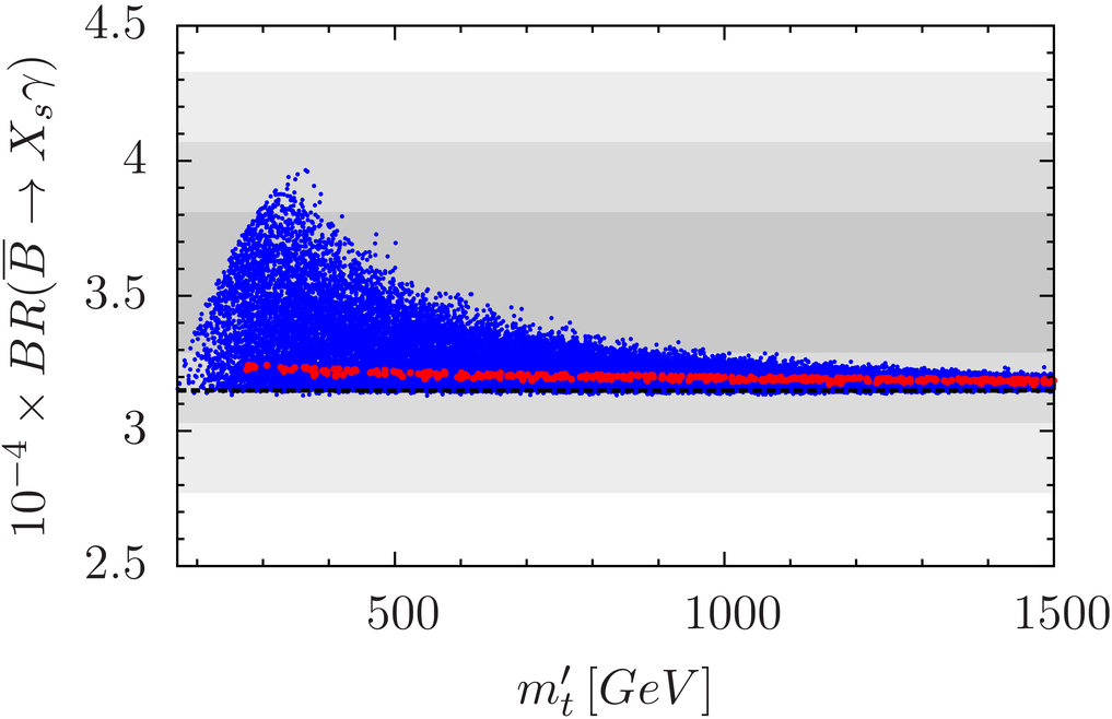
    The impact of the new neutral current-current operators, arising from integrating out the heavy flavour gauge bosons, to the Bยฏโ†’Xsโ€‹ฮณโ†’ยฏ๐ตsubscript๐‘‹๐‘ ๐›พ\bar{B}\to X_{s}\gamma has been studied in Ref.ย [17] and we apply those results to the model.

  • -

    We point out that for a value of |Vuโ€‹b|subscript๐‘‰๐‘ข๐‘|V_{ub}| close to its determination from exclusive decays, i.e. in the ballpark of 3.5ร—10โˆ’33.5superscript1033.5\times 10^{-3}, the model can solve the present tension between ฮตKsubscript๐œ€๐พ\varepsilon_{K} and Sฯˆโ€‹KSsubscript๐‘†๐œ“subscript๐พ๐‘†S_{\psi K_{S}}. For slightly larger values of |Vuโ€‹b|subscript๐‘‰๐‘ข๐‘|V_{ub}|, the model can still accommodate the considered observables within the errors, but for the inclusive determination of |Vuโ€‹b|subscript๐‘‰๐‘ข๐‘|V_{ub}| it suffers from tensions similar to the SM.

  • -

    We scan over all NP parameters and present a correlated analysis of ฮตKsubscript๐œ€๐พ\varepsilon_{K}, the mass differences ฮ”โ€‹MBd,sฮ”subscript๐‘€subscript๐ต๐‘‘๐‘ \Delta M_{B_{d,s}} the B+โ†’ฯ„+โ€‹ฮฝโ†’superscript๐ตsuperscript๐œ๐œˆB^{+}\to\tau^{+}\nu and Bยฏโ†’Xsโ€‹ฮณโ†’ยฏ๐ตsubscript๐‘‹๐‘ ๐›พ\bar{B}\to X_{s}\gamma decays, the ratio ฮ”โ€‹MBd/ฮ”โ€‹MBsฮ”subscript๐‘€subscript๐ต๐‘‘ฮ”subscript๐‘€subscript๐ต๐‘ \Delta M_{B_{d}}/\Delta M_{B_{s}}, the mixing-induced CP asymmetries Sฯˆโ€‹KSsubscript๐‘†๐œ“subscript๐พ๐‘†S_{\psi K_{S}} and Sฯˆโ€‹ฯ•subscript๐‘†๐œ“italic-ฯ•S_{\psi\phi}, and the b๐‘b semileptonic CP-asymmetry Asโ€‹lbsubscriptsuperscript๐ด๐‘๐‘ ๐‘™A^{b}_{sl}.

  • -

    We find that large corrections to the CP observables in the meson oscillations, ฮตKsubscript๐œ€๐พ\varepsilon_{K}, Sฯˆโ€‹Kssubscript๐‘†๐œ“subscript๐พ๐‘ S_{\psi K_{s}} and Sฯˆโ€‹ฯ•subscript๐‘†๐œ“italic-ฯ•S_{\psi\phi}, are allowed. However, requiring ฮตKsubscript๐œ€๐พ\varepsilon_{K} to stay inside its 3โ€‹ฯƒ3๐œŽ3\sigma error range, only small deviations from the SM values of Sฯˆโ€‹Kssubscript๐‘†๐œ“subscript๐พ๐‘ S_{\psi K_{s}} and Sฯˆโ€‹ฯ•subscript๐‘†๐œ“italic-ฯ•S_{\psi\phi} are allowed.

  • -

    We find that requiring ฮตKsubscript๐œ€๐พ\varepsilon_{K}โ€“Sฯˆโ€‹KSsubscript๐‘†๐œ“subscript๐พ๐‘†S_{\psi K_{S}} tension to be removed in this model implies the values of ฮ”โ€‹MBdฮ”subscript๐‘€subscript๐ต๐‘‘\Delta M_{B_{d}} and ฮ”โ€‹MBsฮ”subscript๐‘€subscript๐ต๐‘ \Delta M_{B_{s}} to be significantly larger than the data. While the inclusion of theoretical and parametric uncertainties and in particular the decrease of the weak decay constants could soften this problem, it appears from the present perspective that the model suffers from a serious ฮตKโˆ’ฮ”โ€‹MBโ€‹s,dsubscript๐œ€๐พฮ”subscript๐‘€๐ต๐‘ ๐‘‘\varepsilon_{K}-\Delta M_{B{s,d}} tension.

  • -

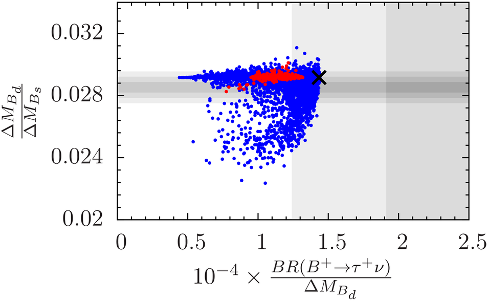
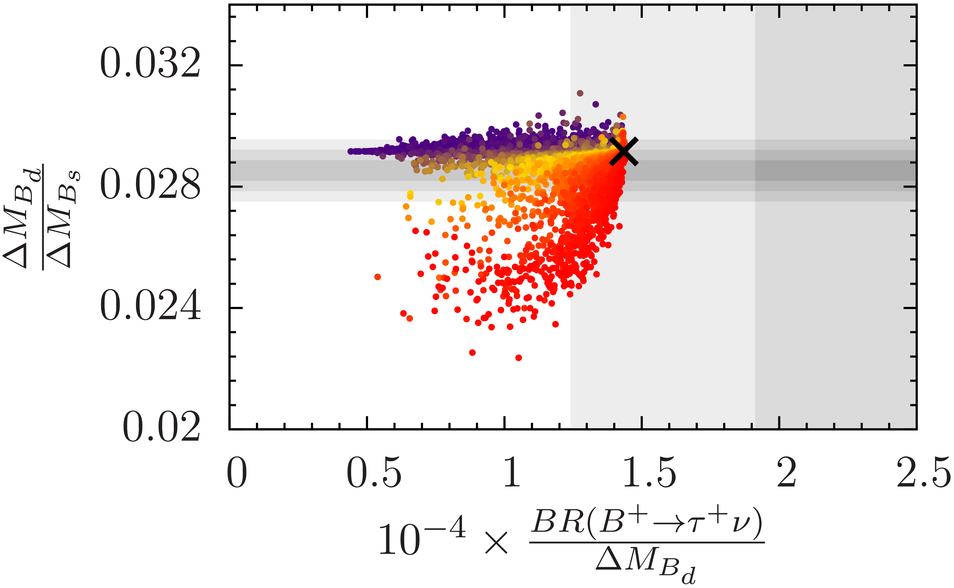
    We also investigate the correlation among two theoretically cleaner observables, ฮ”โ€‹MBd/ฮ”โ€‹MBsฮ”subscript๐‘€subscript๐ต๐‘‘ฮ”subscript๐‘€subscript๐ต๐‘ \Delta M_{B_{d}}/\Delta M_{B_{s}} and Bโ€‹Rโ€‹(B+โ†’ฯ„+โ€‹ฮฝ)/ฮ”โ€‹MBd๐ต๐‘…โ†’superscript๐ตsuperscript๐œ๐œˆฮ”subscript๐‘€subscript๐ต๐‘‘BR(B^{+}\to\tau^{+}\nu)/\Delta M_{B_{d}}. In this way, we strongly constrain the parameter space of the model and conclude that the tension in Bโ€‹Rโ€‹(B+โ†’ฯ„+โ€‹ฮฝ)๐ต๐‘…โ†’superscript๐ตsuperscript๐œ๐œˆBR(B^{+}\to\tau^{+}\nu), present already within the SM, is even increased.

  • -

    We compare the patterns of flavour violation in this model with those found in the original MFV, the MFV with the addition of flavour blind phases and MFV in the left-right asymmetric framework.

  • -

    As a by-product of our work we present a rather complete list of Feynman rules relevant for processes in the quark sector.

The structure of the paper is shown in the table of contents.

2 The Model

In this section we summarise the relevant features of the MGF construction presented in Ref.ย [12], dealing only with the quark sector. The flavour symmetry is that of eq.ย (1.1), but it is gauged. The spectrum is enriched by the corresponding flavour gauge bosons and by new exotic quarks, necessary to cancel the anomalies: in particular the new quarks are two coloured RH Sโ€‹Uโ€‹(3)QL๐‘†๐‘ˆsubscript3subscript๐‘„๐ฟSU(3)_{Q_{L}}-triplets, one LH Sโ€‹Uโ€‹(3)UR๐‘†๐‘ˆsubscript3subscript๐‘ˆ๐‘…SU(3)_{U_{R}}-triplet and one LH Sโ€‹Uโ€‹(3)DR๐‘†๐‘ˆsubscript3subscript๐ท๐‘…SU(3)_{D_{R}}-triplet. In table 1, we list all the fields present in the theory and their transformation properties under the gauge groups.

QLsubscript๐‘„๐ฟQ_{L} URsubscript๐‘ˆ๐‘…U_{R} DRsubscript๐ท๐‘…D_{R} H๐ปH ฮจuRsubscriptฮจsubscript๐‘ข๐‘…\Psi_{u_{R}} ฮจdRsubscriptฮจsubscript๐‘‘๐‘…\Psi_{d_{R}} ฮจuLsubscriptฮจsubscript๐‘ข๐ฟ\Psi_{u_{L}} ฮจdLsubscriptฮจsubscript๐‘‘๐ฟ\Psi_{d_{L}} Yusubscript๐‘Œ๐‘ขY_{u} Ydsubscript๐‘Œ๐‘‘Y_{d}
Sโ€‹Uโ€‹(3)c๐‘†๐‘ˆsubscript3๐‘SU(3)_{c} ๐Ÿ‘3\bf 3 ๐Ÿ‘3\bf 3 ๐Ÿ‘3\bf 3 ๐Ÿ1\bf 1 ๐Ÿ‘3\bf 3 ๐Ÿ‘3\bf 3 ๐Ÿ‘3\bf 3 ๐Ÿ‘3\bf 3 ๐Ÿ1\bf 1 ๐Ÿ1\bf 1
Sโ€‹Uโ€‹(2)L๐‘†๐‘ˆsubscript2๐ฟSU(2)_{L} ๐Ÿ2\bf 2 ๐Ÿ1\bf 1 ๐Ÿ1\bf 1 ๐Ÿ2\bf 2 ๐Ÿ1\bf 1 ๐Ÿ1\bf 1 ๐Ÿ1\bf 1 ๐Ÿ1\bf 1 ๐Ÿ1\bf 1 ๐Ÿ1\bf 1
Uโ€‹(1)Y๐‘ˆsubscript1๐‘ŒU(1)_{Y} +1โฃ/6superscript1subscript6+^{1}/_{6} +2โฃ/3superscript2subscript3+^{2}/_{3} โˆ’1โฃ/3superscript1subscript3-^{1}/_{3} +1โฃ/2superscript1subscript2+^{1}/_{2} +2โฃ/3superscript2subscript3+^{2}/_{3} โˆ’1โฃ/3superscript1subscript3-^{1}/_{3} +2โฃ/3superscript2subscript3+^{2}/_{3} โˆ’1โฃ/3superscript1subscript3-^{1}/_{3} 00 00
Sโ€‹Uโ€‹(3)QL๐‘†๐‘ˆsubscript3subscript๐‘„๐ฟSU(3)_{Q_{L}} ๐Ÿ‘3\bf 3 ๐Ÿ1\bf 1 ๐Ÿ1\bf 1 ๐Ÿ1\bf 1 ๐Ÿ‘3\bf 3 ๐Ÿ‘3\bf 3 ๐Ÿ1\bf 1 ๐Ÿ1\bf 1 ๐Ÿ‘ยฏยฏ3\bf\overline{3} ๐Ÿ‘ยฏยฏ3\bf\overline{3}
Sโ€‹Uโ€‹(3)UR๐‘†๐‘ˆsubscript3subscript๐‘ˆ๐‘…SU(3)_{U_{R}} ๐Ÿ1\bf 1 ๐Ÿ‘3\bf 3 ๐Ÿ1\bf 1 ๐Ÿ1\bf 1 ๐Ÿ1\bf 1 ๐Ÿ1\bf 1 ๐Ÿ‘3\bf 3 ๐Ÿ1\bf 1 ๐Ÿ‘3\bf 3 ๐Ÿ1\bf 1
Sโ€‹Uโ€‹(3)DR๐‘†๐‘ˆsubscript3subscript๐ท๐‘…SU(3)_{D_{R}} ๐Ÿ1\bf 1 ๐Ÿ1\bf 1 ๐Ÿ‘3\bf 3 ๐Ÿ1\bf 1 ๐Ÿ1\bf 1 ๐Ÿ1\bf 1 ๐Ÿ1\bf 1 ๐Ÿ‘3\bf 3 ๐Ÿ1\bf 1 ๐Ÿ‘3\bf 3
Table 1: The transformation properties of the fields under the SM and flavour gauge symmetries.

With this matter content, the most general renormalisable Lagrangian invariant under the SM and flavour gauge groups can be divided into three parts:

โ„’=โ„’kโ€‹iโ€‹n+โ„’iโ€‹nโ€‹tโˆ’Vโ€‹[H,Yu,Yd].โ„’subscriptโ„’๐‘˜๐‘–๐‘›subscriptโ„’๐‘–๐‘›๐‘ก๐‘‰๐ปsubscript๐‘Œ๐‘ขsubscript๐‘Œ๐‘‘\mathcal{L}=\mathcal{L}_{kin}+\mathcal{L}_{int}-V\left[H,Y_{u},Y_{d}\right]\,. (2.1)

The first one, โ„’kโ€‹iโ€‹nsubscriptโ„’๐‘˜๐‘–๐‘›\mathcal{L}_{kin}, contains the kinetic terms of all the fields and the couplings of fermions and scalar bosons to the gauge bosons. The covariant derivative entering โ„’kโ€‹iโ€‹nsubscriptโ„’๐‘˜๐‘–๐‘›\mathcal{L}_{kin} accounts for SM gauge boson-fermion interactions and additional flavour interactions involving new gauge bosons and fermions:

DฮผโŠƒโˆ‘f=Q,U,Diโ€‹gfโ€‹Nfโ€‹(Af)ฮผ,(Af)ฮผโ‰กโˆ‘a=18(Afa)ฮผโ€‹ฮปSโ€‹Uโ€‹(3)a2,formulae-sequencesubscript๐‘“๐‘„๐‘ˆ๐ท๐‘–subscript๐‘”๐‘“subscript๐‘๐‘“subscriptsubscript๐ด๐‘“๐œ‡subscript๐ท๐œ‡subscriptsubscript๐ด๐‘“๐œ‡superscriptsubscript๐‘Ž18subscriptsuperscriptsubscript๐ด๐‘“๐‘Ž๐œ‡superscriptsubscript๐œ†๐‘†๐‘ˆ3๐‘Ž2D_{\mu}\supset\sum_{f=Q,U,D}i\,g_{f}\,N_{f}\,(A_{f})_{\mu}\,,\qquad\qquad\qquad(A_{f})_{\mu}\equiv\sum_{a=1}^{8}(A_{f}^{a})_{\mu}\dfrac{\lambda_{SU(3)}^{a}}{2}\,, (2.2)

where gfsubscript๐‘”๐‘“g_{f} are the flavour gauge coupling constants, Nfsubscript๐‘๐‘“N_{f} the quantum numbers, Afasuperscriptsubscript๐ด๐‘“๐‘ŽA_{f}^{a} the flavour gauge bosons and ฮปSโ€‹Uโ€‹(3)asuperscriptsubscript๐œ†๐‘†๐‘ˆ3๐‘Ž\lambda_{SU(3)}^{a} the Gell-Mann matrices.

The second term in eq.ย (2.1), โ„’iโ€‹nโ€‹tsubscriptโ„’๐‘–๐‘›๐‘ก\mathcal{L}_{int}, contains the quark mass terms and the quark-scalar interactions:

โ„’int=ฮปuโ€‹QยฏLโ€‹H~โ€‹ฮจuR+ฮปuโ€ฒโ€‹ฮจยฏuLโ€‹Yuโ€‹ฮจuR+Muโ€‹ฮจยฏuLโ€‹UR++ฮปdโ€‹QยฏLโ€‹Hโ€‹ฮจdR+ฮปuโ€ฒโ€‹ฮจยฏdLโ€‹Ydโ€‹ฮจdR+Mdโ€‹ฮจยฏdLโ€‹DR+h.c.,subscriptโ„’intsubscript๐œ†๐‘ขsubscriptยฏ๐‘„๐ฟ~๐ปsubscriptฮจsubscript๐‘ข๐‘…superscriptsubscript๐œ†๐‘ขโ€ฒsubscriptยฏฮจsubscript๐‘ข๐ฟsubscript๐‘Œ๐‘ขsubscriptฮจsubscript๐‘ข๐‘…subscript๐‘€๐‘ขsubscriptยฏฮจsubscript๐‘ข๐ฟsubscript๐‘ˆ๐‘…subscript๐œ†๐‘‘subscriptยฏ๐‘„๐ฟ๐ปsubscriptฮจsubscript๐‘‘๐‘…superscriptsubscript๐œ†๐‘ขโ€ฒsubscriptยฏฮจsubscript๐‘‘๐ฟsubscript๐‘Œ๐‘‘subscriptฮจsubscript๐‘‘๐‘…subscript๐‘€๐‘‘subscriptยฏฮจsubscript๐‘‘๐ฟsubscript๐ท๐‘…h.c.\begin{split}\mathcal{L}_{\text{int}}=&\;\;\lambda_{u}\,\overline{Q}_{L}\tilde{H}\,\Psi_{u_{R}}+\lambda_{u}^{\prime}\overline{\Psi}_{u_{L}}Y_{u}\,\Psi_{u_{R}}+M_{u}\,\overline{\Psi}_{u_{L}}U_{R}+\\[5.69054pt] &+\lambda_{d}\,\overline{Q}_{L}H\,\Psi_{d_{R}}+\lambda_{u}^{\prime}\overline{\Psi}_{d_{L}}Y_{d}\,\Psi_{d_{R}}+M_{d}\,\overline{\Psi}_{d_{L}}D_{R}+\text{h.c.}\,,\end{split} (2.3)

where Mu,dsubscript๐‘€๐‘ข๐‘‘M_{u,d} are universal mass parameters and ฮปu,d(โ€ฒ)subscriptsuperscript๐œ†โ€ฒ๐‘ข๐‘‘\lambda^{(\prime)}_{u,d} are universal coupling constants that can be chosen real, through a redefinition of the fields.

The last term in eq.ย (2.1), Vโ€‹[H,Yu,Yd]๐‘‰๐ปsubscript๐‘Œ๐‘ขsubscript๐‘Œ๐‘‘V\left[H,Y_{u},Y_{d}\right], is the scalar potential of the model, containing the SM Higgs and the flavons Yu,dsubscript๐‘Œ๐‘ข๐‘‘Y_{u,d}. The mechanisms of both electroweak and flavour symmetry breaking arise from the minimisation of this scalar potential. It has not been explicitly constructed in Ref.ย [12] and it is beyond the scope of the present paper to provide such a scalar potential (see Ref.ย [16] for a recent analysis). Therefore, we assume that the spontaneous breaking of the electroweak symmetry proceeds as in the SM through the Higgs mechanism and that the spontaneous flavour symmetry breaking is driven by the flavon fields Yu,dsubscript๐‘Œ๐‘ข๐‘‘Y_{u,d} which develop the following VEVs:

โŸจYdโŸฉ=Y^d,โŸจYuโŸฉ=Y^uโ€‹V.formulae-sequencedelimited-โŸจโŸฉsubscript๐‘Œ๐‘‘subscript^๐‘Œ๐‘‘delimited-โŸจโŸฉsubscript๐‘Œ๐‘ขsubscript^๐‘Œ๐‘ข๐‘‰\langle Y_{d}\rangle=\hat{Y}_{d}\,,\qquad\qquad\langle Y_{u}\rangle=\hat{Y}_{u}\,V\,. (2.4)

Here Y^u,dsubscript^๐‘Œ๐‘ข๐‘‘\hat{Y}_{u,d} are diagonal 3ร—3333\times 3 matrices and V๐‘‰V is a unitary matrix. We emphasise that, despite the similarity to eq.ย (1.5) of MFV, the matrix V๐‘‰V is not the CKM matrix and the vacuum expectation values โŸจYu,dโŸฉdelimited-โŸจโŸฉsubscript๐‘Œ๐‘ข๐‘‘\left\langle Y_{u,d}\right\rangle do not coincide with the SM Yukawa matrices. This is illustrated by moving to the fermion-mass eigenbasis. In what follows we focus on the up-quark sector, but analogous formulae can also be written for the down-quark sector. The LH and RH up-quarks mix separately giving rise to SM up-quarks uR,Lisubscriptsuperscript๐‘ข๐‘–๐‘…๐ฟu^{i}_{R,L} and exotic up-quarks uR,Lโ€ฒโฃisubscriptsuperscript๐‘ขโ€ฒ๐‘–๐‘…๐ฟu^{\prime i}_{R,L}:

(uR,LiuR,Lโ€ฒโฃi)=(cu(R,L)โ€‹iโˆ’su(R,L)โ€‹isu(R,L)โ€‹icu(R,L)โ€‹i)โ€‹(UR,LiฮจuR,Li),matrixsubscriptsuperscript๐‘ข๐‘–๐‘…๐ฟsubscriptsuperscript๐‘ขโ€ฒ๐‘–๐‘…๐ฟmatrixsubscript๐‘subscript๐‘ข๐‘…๐ฟ๐‘–subscript๐‘ subscript๐‘ข๐‘…๐ฟ๐‘–subscript๐‘ subscript๐‘ข๐‘…๐ฟ๐‘–subscript๐‘subscript๐‘ข๐‘…๐ฟ๐‘–matrixsubscriptsuperscript๐‘ˆ๐‘–๐‘…๐ฟsubscriptsuperscriptฮจ๐‘–subscript๐‘ข๐‘…๐ฟ\begin{pmatrix}u^{i}_{R,L}\\[5.69054pt] u^{\prime i}_{R,L}\end{pmatrix}=\begin{pmatrix}c_{u_{(R,L)i}}&-s_{u_{(R,L)i}}\\[5.69054pt] s_{u_{(R,L)i}}&c_{u_{(R,L)i}}\end{pmatrix}\begin{pmatrix}U^{i}_{R,L}\\[5.69054pt] \Psi^{i}_{u_{R,L}}\end{pmatrix}\,, (2.5)

where cu(R,L)โ€‹isubscript๐‘subscript๐‘ข๐‘…๐ฟ๐‘–c_{u_{(R,L)i}} and su(R,L)โ€‹isubscript๐‘ subscript๐‘ข๐‘…๐ฟ๐‘–s_{u_{(R,L)i}} are cosines and sines, respectively. Denoting with mfisubscript๐‘šsuperscript๐‘“๐‘–m_{f^{i}} the mass of the up-type fi={ui,uโ€ฒโฃi}superscript๐‘“๐‘–superscript๐‘ข๐‘–superscript๐‘ขโ€ฒ๐‘–f^{i}=\{u^{i},\,u^{\prime i}\} quark, what follows is a direct inverse proportionality between muisubscript๐‘šsuperscript๐‘ข๐‘–m_{u^{i}} and muโ€ฒโฃisubscript๐‘šsuperscript๐‘ขโ€ฒ๐‘–m_{u^{\prime i}}:

muiโ€‹muโ€ฒโฃi=Muโ€‹ฮปuโ€‹v2.subscript๐‘šsuperscript๐‘ข๐‘–subscript๐‘šsuperscript๐‘ขโ€ฒ๐‘–subscript๐‘€๐‘ขsubscript๐œ†๐‘ข๐‘ฃ2m_{u^{i}}\,m_{u^{\prime i}}=M_{u}\,\lambda_{u}\,\dfrac{v}{\sqrt{2}}\,. (2.6)

We can express these masses in terms of the flavour symmetry breaking parameters:

mui=suRโ€‹iโ€‹suLโ€‹icuRโ€‹i2โˆ’suLโ€‹i2โ€‹ฮปuโ€ฒโ€‹(Y^u)i,muโ€ฒโฃi=cuRโ€‹iโ€‹cuLโ€‹icuRโ€‹i2โˆ’suLโ€‹i2โ€‹ฮปuโ€ฒโ€‹(Y^u)i,formulae-sequencesubscript๐‘šsuperscript๐‘ข๐‘–subscript๐‘ subscript๐‘ข๐‘…๐‘–subscript๐‘ subscript๐‘ข๐ฟ๐‘–subscriptsuperscript๐‘2subscript๐‘ข๐‘…๐‘–subscriptsuperscript๐‘ 2subscript๐‘ข๐ฟ๐‘–subscriptsuperscript๐œ†โ€ฒ๐‘ขsubscriptsubscript^๐‘Œ๐‘ข๐‘–subscript๐‘šsuperscript๐‘ขโ€ฒ๐‘–subscript๐‘subscript๐‘ข๐‘…๐‘–subscript๐‘subscript๐‘ข๐ฟ๐‘–subscriptsuperscript๐‘2subscript๐‘ข๐‘…๐‘–subscriptsuperscript๐‘ 2subscript๐‘ข๐ฟ๐‘–subscriptsuperscript๐œ†โ€ฒ๐‘ขsubscriptsubscript^๐‘Œ๐‘ข๐‘–m_{u^{i}}=\dfrac{s_{u_{Ri}}\,s_{u_{Li}}}{c^{2}_{u_{Ri}}-s^{2}_{u_{Li}}}\lambda^{\prime}_{u}(\hat{Y}_{u})_{i}\,,\qquad\qquad m_{u^{\prime i}}=\dfrac{c_{u_{Ri}}\,c_{u_{Li}}}{c^{2}_{u_{Ri}}-s^{2}_{u_{Li}}}\lambda^{\prime}_{u}(\hat{Y}_{u})_{i}\,, (2.7)

where a straightforward calculation gives

suLโ€‹i=muiMuโ€‹|ฮปuโ€‹vโ€‹muโ€ฒโฃiโˆ’2โ€‹Muโ€‹mui2โ€‹(muโ€ฒโฃi2โˆ’mui2)|,suRโ€‹i=muiฮปuโ€‹vโ€‹|2โ€‹Muโ€‹muโ€ฒโฃiโˆ’ฮปuโ€‹vโ€‹muimuโ€ฒโฃi2โˆ’mui2|.formulae-sequencesubscript๐‘ subscript๐‘ข๐ฟ๐‘–subscript๐‘šsuperscript๐‘ข๐‘–subscript๐‘€๐‘ขsubscript๐œ†๐‘ข๐‘ฃsubscript๐‘šsuperscript๐‘ขโ€ฒ๐‘–2subscript๐‘€๐‘ขsubscript๐‘šsuperscript๐‘ข๐‘–2subscriptsuperscript๐‘š2superscript๐‘ขโ€ฒ๐‘–subscriptsuperscript๐‘š2superscript๐‘ข๐‘–subscript๐‘ subscript๐‘ข๐‘…๐‘–subscript๐‘šsuperscript๐‘ข๐‘–subscript๐œ†๐‘ข๐‘ฃ2subscript๐‘€๐‘ขsubscript๐‘šsuperscript๐‘ขโ€ฒ๐‘–subscript๐œ†๐‘ข๐‘ฃsubscript๐‘šsuperscript๐‘ข๐‘–subscriptsuperscript๐‘š2superscript๐‘ขโ€ฒ๐‘–subscriptsuperscript๐‘š2superscript๐‘ข๐‘–s_{u_{Li}}=\sqrt{\dfrac{m_{u^{i}}}{M_{u}}\left|\dfrac{\lambda_{u}\,v\,m_{u^{\prime i}}-\sqrt{2}\,M_{u}\,m_{u^{i}}}{\sqrt{2}\,\left(m^{2}_{u^{\prime i}}-m^{2}_{u^{i}}\right)}\right|}\,,\quad\quad s_{u_{Ri}}=\sqrt{\dfrac{m_{u^{i}}}{\lambda_{u}\,v}\left|\dfrac{\sqrt{2}\,M_{u}\,m_{u^{\prime i}}-\lambda_{u}\,v\,m_{u^{i}}}{m^{2}_{u^{\prime i}}-m^{2}_{u^{i}}}\right|}\,. (2.8)

These results are exact and valid for all quark generations. However, taking the limit muโ€ฒโฃiโ‰ซmuimuch-greater-thansubscript๐‘šsuperscript๐‘ขโ€ฒ๐‘–subscript๐‘šsuperscript๐‘ข๐‘–m_{u^{\prime i}}\gg m_{u^{i}}, we find simple formulae that transparently expose the behaviour of the previous expressions. In this limit we find

muiโ‰ˆv2โ€‹ฮปuโ€‹Muฮปuโ€ฒโ€‹(Y^u)i,subscript๐‘šsuperscript๐‘ข๐‘–๐‘ฃ2subscript๐œ†๐‘ขsubscript๐‘€๐‘ขsubscriptsuperscript๐œ†โ€ฒ๐‘ขsubscriptsubscript^๐‘Œ๐‘ข๐‘–\displaystyle m_{u^{i}}\approx\dfrac{v}{\sqrt{2}}\dfrac{\lambda_{u}\,M_{u}}{\lambda^{\prime}_{u}\,(\hat{Y}_{u})_{i}}\,,\qquad\qquad muโ€ฒโฃiโ‰ˆฮปuโ€ฒโ€‹(Y^u)i,subscript๐‘šsuperscript๐‘ขโ€ฒ๐‘–subscriptsuperscript๐œ†โ€ฒ๐‘ขsubscriptsubscript^๐‘Œ๐‘ข๐‘–\displaystyle m_{u^{\prime i}}\approx\lambda^{\prime}_{u}\,(\hat{Y}_{u})_{i}\,, (2.9)
suLโ€‹iโ‰ˆmuimuโ€ฒโฃiโ€‹ฮปuโ€‹v2โ€‹Mu,subscript๐‘ subscript๐‘ข๐ฟ๐‘–subscript๐‘šsuperscript๐‘ข๐‘–subscript๐‘šsuperscript๐‘ขโ€ฒ๐‘–subscript๐œ†๐‘ข๐‘ฃ2subscript๐‘€๐‘ข\displaystyle s_{u_{Li}}\approx\sqrt{\dfrac{m_{u^{i}}}{m_{u^{\prime i}}}\dfrac{\lambda_{u}\,v}{\sqrt{2}\,M_{u}}}\,,\qquad\qquad suRโ€‹iโ‰ˆmuimuโ€ฒโฃiโ€‹2โ€‹Muฮปuโ€‹v,subscript๐‘ subscript๐‘ข๐‘…๐‘–subscript๐‘šsuperscript๐‘ข๐‘–subscript๐‘šsuperscript๐‘ขโ€ฒ๐‘–2subscript๐‘€๐‘ขsubscript๐œ†๐‘ข๐‘ฃ\displaystyle s_{u_{Ri}}\approx\sqrt{\dfrac{m_{u^{i}}}{m_{u^{\prime i}}}\dfrac{\sqrt{2}\,M_{u}}{\lambda_{u}\,v}}\,, (2.10)

as it is in the usual see-saw scheme in the limit of (Y^u)iโ‰ซMu,vmuch-greater-thansubscriptsubscript^๐‘Œ๐‘ข๐‘–subscript๐‘€๐‘ข๐‘ฃ(\hat{Y}_{u})_{i}\gg M_{u}\,,v. These simplified relations are valid for all the fermions, apart from the top-quark for which the condition mtโ€ฒโ‰ซmtmuch-greater-thansubscript๐‘šsuperscript๐‘กโ€ฒsubscript๐‘š๐‘กm_{t^{\prime}}\gg m_{t} is not satisfied and large corrections to eq.ย (2.10) are expected.

From eq.ย (2.10) we see that to reproduce the correct SM quark spectrum, Y^usubscript^๐‘Œ๐‘ข\hat{Y}_{u} must have an inverted hierarchy with respect to the SM Yukawas.

The presence of new exotic quarks has a relevant impact on the SM couplings. Indeed, the charged current-current interactions including SM and heavy quarks are governed by a 6ร—6666\times 6 matrix which is constructed from the unitary 3ร—3333\times 3 matrix V๐‘‰V of eq.ย (2.4) and the cuLโ€‹isubscript๐‘subscript๐‘ข๐ฟ๐‘–c_{u_{Li}}, cdLโ€‹isubscript๐‘subscript๐‘‘๐ฟ๐‘–c_{d_{Li}}, suLโ€‹isubscript๐‘ subscript๐‘ข๐ฟ๐‘–s_{u_{Li}} and sdLโ€‹isubscript๐‘ subscript๐‘‘๐ฟ๐‘–s_{d_{Li}} with (i=1,2,3๐‘–123i=1,2,3) introduced above. Adopting a matrix notation, the non-unitary 3ร—3333\times 3 matrices

cuLโ€‹Vโ€‹cdL,suLโ€‹Vโ€‹sdLsubscript๐‘subscript๐‘ข๐ฟ๐‘‰subscript๐‘subscript๐‘‘๐ฟsubscript๐‘ subscript๐‘ข๐ฟ๐‘‰subscript๐‘ subscript๐‘‘๐ฟc_{u_{L}}\,V\,c_{d_{L}}\,,\quad\quad s_{u_{L}}\,V\,s_{d_{L}} (2.11)

describe the charged (W+superscript๐‘ŠW^{+}) current-current interactions within the light and heavy systems, respectively. The analogous matrices

cuLโ€‹Vโ€‹sdL,suLโ€‹Vโ€‹cdLsubscript๐‘subscript๐‘ข๐ฟ๐‘‰subscript๐‘ subscript๐‘‘๐ฟsubscript๐‘ subscript๐‘ข๐ฟ๐‘‰subscript๐‘subscript๐‘‘๐ฟc_{u_{L}}\,V\,s_{d_{L}}\,,\quad\quad s_{u_{L}}\,V\,c_{d_{L}} (2.12)

describe the charged current-current interactions between light and heavy fermions. In this notation, cu,dLsubscript๐‘๐‘ขsubscript๐‘‘๐ฟc_{{u,d}_{L}} and su,dLsubscript๐‘ ๐‘ขsubscript๐‘‘๐ฟs_{{u,d}_{L}} are diagonal matrices, whose entries are cu,dLโ€‹isubscript๐‘๐‘ขsubscript๐‘‘๐ฟ๐‘–c_{{u,d}_{Li}} and su,dLโ€‹isubscript๐‘ ๐‘ขsubscript๐‘‘๐ฟ๐‘–s_{{u,d}_{Li}}, respectively. Moreover, we point out that in the no-mixing limit, cu,dLโ€‹iโ†’1โ†’subscript๐‘๐‘ขsubscript๐‘‘๐ฟ๐‘–1c_{{u,d}_{Li}}\to 1 and su,dLโ€‹iโ†’0โ†’subscript๐‘ ๐‘ขsubscript๐‘‘๐ฟ๐‘–0s_{{u,d}_{Li}}\to 0, the (non-unitary) 6ร—6666\times 6 matrix reduces to

(V000).matrix๐‘‰000\begin{pmatrix}V&0\\[5.69054pt] 0&0\end{pmatrix}\,. (2.13)

In this case the CKM matrix coincides with the unitary matrix V๐‘‰V. As soon as the mixing is switched on, the CKM is modified to include cu,dLsubscript๐‘๐‘ขsubscript๐‘‘๐ฟc_{{u,d}_{L}}, which breaks unitarity. However, these deviations from unitarity are quite small (see sec.ย 6.2.2). Moreover no new CP violating phases appear in the resulting CKM matrix. At first sight their absence implies no impact of new contributions to the CP-violating observables Sฯˆโ€‹Kssubscript๐‘†๐œ“subscript๐พ๐‘ S_{\psi K_{s}} and Sฯˆโ€‹ฯ•subscript๐‘†๐œ“italic-ฯ•S_{\psi\phi}. However, this is not the case due to the modification of the CKM matrix and the presence of flavour gauge bosons. In this respect, this framework does differ from the original MFV of Ref.ย [8].

A consequence of the modification of the CKM matrix is the breaking of the GIM mechanism if only SM quarks are considered in loop-induced processes. However, once also the exotic quarks are included the GIM mechanism is recovered. We return to this issue in sec.ย 3.4.

The interactions with the Z๐‘Z boson and the Higgs field are modified too. Their effects have been already discussed in Ref.ย [12] and it turned out that the largest constraint comes from the modified Zโ€‹bโ€‹bยฏ๐‘๐‘ยฏ๐‘Z\,b\,\bar{b} coupling.

Once the flavour symmetry is spontaneously broken by the flavon VEVs, the flavour gauge bosons acquire masses and mix among themselves. Using the vector notation for the flavour gauge bosons,

ฯ‡=(AQ1,โ€ฆ,AQ8,AU1,โ€ฆ,AU8,AD1,โ€ฆ,AD8)T,๐œ’superscriptsuperscriptsubscript๐ด๐‘„1โ€ฆsuperscriptsubscript๐ด๐‘„8superscriptsubscript๐ด๐‘ˆ1โ€ฆsuperscriptsubscript๐ด๐‘ˆ8superscriptsubscript๐ด๐ท1โ€ฆsuperscriptsubscript๐ด๐ท8๐‘‡\chi=\left(A_{Q}^{1},\ldots,A_{Q}^{8},A_{U}^{1},\ldots,A_{U}^{8},A_{D}^{1},\ldots,A_{D}^{8}\right)^{T}\,, (2.14)

the corresponding mass Lagrangian reads

โ„’mass=12โ€‹ฯ‡Tโ€‹โ„ณA2โ€‹ฯ‡withโ„ณA2=(MQโ€‹Q2MQโ€‹U2MQโ€‹D2MUโ€‹Q2MUโ€‹U20MDโ€‹Q20MDโ€‹D2),formulae-sequencesubscriptโ„’mass12superscript๐œ’๐‘‡superscriptsubscriptโ„ณ๐ด2๐œ’withsuperscriptsubscriptโ„ณ๐ด2matrixsubscriptsuperscript๐‘€2๐‘„๐‘„subscriptsuperscript๐‘€2๐‘„๐‘ˆsubscriptsuperscript๐‘€2๐‘„๐ทsubscriptsuperscript๐‘€2๐‘ˆ๐‘„subscriptsuperscript๐‘€2๐‘ˆ๐‘ˆ0subscriptsuperscript๐‘€2๐ท๐‘„0subscriptsuperscript๐‘€2๐ท๐ท\mathcal{L}_{\text{mass}}=\dfrac{1}{2}\,\chi^{T}\,{\cal M}_{A}^{2}\,\chi\,\qquad\text{with}\qquad{\cal M}_{A}^{2}=\begin{pmatrix}M^{2}_{QQ}&M^{2}_{QU}&M^{2}_{QD}\\[2.84526pt] M^{2}_{UQ}&M^{2}_{UU}&0\\[2.84526pt] M^{2}_{DQ}&0&M^{2}_{DD}\end{pmatrix}\,, (2.15)

and

(MQโ€‹Q2)aโ€‹b=subscriptsubscriptsuperscript๐‘€2๐‘„๐‘„๐‘Ž๐‘absent\displaystyle\left(M^{2}_{QQ}\right)_{ab}= 14โ€‹gQ2โ€‹Trโ€‹[โŸจYuโŸฉโ€‹{ฮปSโ€‹Uโ€‹(3)a,ฮปSโ€‹Uโ€‹(3)b}โ€‹โŸจYuโŸฉโ€ +โŸจYdโŸฉโ€‹{ฮปSโ€‹Uโ€‹(3)a,ฮปSโ€‹Uโ€‹(3)b}โ€‹โŸจYdโŸฉโ€ ]14superscriptsubscript๐‘”๐‘„2Trdelimited-[]delimited-โŸจโŸฉsubscript๐‘Œ๐‘ขsuperscriptsubscript๐œ†๐‘†๐‘ˆ3๐‘Žsuperscriptsubscript๐œ†๐‘†๐‘ˆ3๐‘superscriptdelimited-โŸจโŸฉsubscript๐‘Œ๐‘ขโ€ delimited-โŸจโŸฉsubscript๐‘Œ๐‘‘superscriptsubscript๐œ†๐‘†๐‘ˆ3๐‘Žsuperscriptsubscript๐œ†๐‘†๐‘ˆ3๐‘superscriptdelimited-โŸจโŸฉsubscript๐‘Œ๐‘‘โ€ \displaystyle\frac{1}{4}\,g_{Q}^{2}\,\text{Tr}\left[\left\langle Y_{u}\right\rangle\left\{\lambda_{SU(3)}^{a},\lambda_{SU(3)}^{b}\right\}\left\langle Y_{u}\right\rangle^{{\dagger}}+\left\langle Y_{d}\right\rangle\left\{\lambda_{SU(3)}^{a},\lambda_{SU(3)}^{b}\right\}\left\langle Y_{d}\right\rangle^{{\dagger}}\right] (2.16)
(MUโ€‹U2)aโ€‹b=subscriptsubscriptsuperscript๐‘€2๐‘ˆ๐‘ˆ๐‘Ž๐‘absent\displaystyle\left(M^{2}_{UU}\right)_{ab}= 14โ€‹gU2โ€‹Trโ€‹[โŸจYuโŸฉโ€‹{ฮปSโ€‹Uโ€‹(3)a,ฮปSโ€‹Uโ€‹(3)b}โ€‹โŸจYuโŸฉโ€ ]14superscriptsubscript๐‘”๐‘ˆ2Trdelimited-[]delimited-โŸจโŸฉsubscript๐‘Œ๐‘ขsuperscriptsubscript๐œ†๐‘†๐‘ˆ3๐‘Žsuperscriptsubscript๐œ†๐‘†๐‘ˆ3๐‘superscriptdelimited-โŸจโŸฉsubscript๐‘Œ๐‘ขโ€ \displaystyle\frac{1}{4}\,g_{U}^{2}\,\text{Tr}\left[\left\langle Y_{u}\right\rangle\left\{\lambda_{SU(3)}^{a},\lambda_{SU(3)}^{b}\right\}\left\langle Y_{u}\right\rangle^{{\dagger}}\right]
(MDโ€‹D2)aโ€‹b=subscriptsubscriptsuperscript๐‘€2๐ท๐ท๐‘Ž๐‘absent\displaystyle\left(M^{2}_{DD}\right)_{ab}= 14โ€‹gD2โ€‹Trโ€‹[โŸจYdโŸฉโ€‹{ฮปSโ€‹Uโ€‹(3)a,ฮปSโ€‹Uโ€‹(3)b}โ€‹โŸจYdโŸฉโ€ ]14superscriptsubscript๐‘”๐ท2Trdelimited-[]delimited-โŸจโŸฉsubscript๐‘Œ๐‘‘superscriptsubscript๐œ†๐‘†๐‘ˆ3๐‘Žsuperscriptsubscript๐œ†๐‘†๐‘ˆ3๐‘superscriptdelimited-โŸจโŸฉsubscript๐‘Œ๐‘‘โ€ \displaystyle\frac{1}{4}\,g_{D}^{2}\,\text{Tr}\left[\left\langle Y_{d}\right\rangle\left\{\lambda_{SU(3)}^{a},\lambda_{SU(3)}^{b}\right\}\left\langle Y_{d}\right\rangle^{{\dagger}}\right]
(MQโ€‹U2)aโ€‹b=subscriptsubscriptsuperscript๐‘€2๐‘„๐‘ˆ๐‘Ž๐‘absent\displaystyle\left(M^{2}_{QU}\right)_{ab}= (MUโ€‹Q2)bโ€‹a=โˆ’12โ€‹gQโ€‹gUโ€‹Trโ€‹[ฮปSโ€‹Uโ€‹(3)aโ€‹โŸจYuโŸฉโ€ โ€‹ฮปSโ€‹Uโ€‹(3)bโ€‹โŸจYuโŸฉ]subscriptsubscriptsuperscript๐‘€2๐‘ˆ๐‘„๐‘๐‘Ž12subscript๐‘”๐‘„subscript๐‘”๐‘ˆTrdelimited-[]superscriptsubscript๐œ†๐‘†๐‘ˆ3๐‘Žsuperscriptdelimited-โŸจโŸฉsubscript๐‘Œ๐‘ขโ€ superscriptsubscript๐œ†๐‘†๐‘ˆ3๐‘delimited-โŸจโŸฉsubscript๐‘Œ๐‘ข\displaystyle\left(M^{2}_{UQ}\right)_{ba}=-\frac{1}{2}\,g_{Q}\,g_{U}\,\text{Tr}\left[\lambda_{SU(3)}^{a}\left\langle Y_{u}\right\rangle^{{\dagger}}\lambda_{SU(3)}^{b}\left\langle Y_{u}\right\rangle\right]
(MQโ€‹D2)aโ€‹b=subscriptsubscriptsuperscript๐‘€2๐‘„๐ท๐‘Ž๐‘absent\displaystyle\left(M^{2}_{QD}\right)_{ab}= (MDโ€‹Q2)bโ€‹a=โˆ’12โ€‹gQโ€‹gDโ€‹Trโ€‹[ฮปSโ€‹Uโ€‹(3)aโ€‹โŸจYdโŸฉโ€ โ€‹ฮปSโ€‹Uโ€‹(3)bโ€‹โŸจYdโŸฉ].subscriptsubscriptsuperscript๐‘€2๐ท๐‘„๐‘๐‘Ž12subscript๐‘”๐‘„subscript๐‘”๐ทTrdelimited-[]superscriptsubscript๐œ†๐‘†๐‘ˆ3๐‘Žsuperscriptdelimited-โŸจโŸฉsubscript๐‘Œ๐‘‘โ€ superscriptsubscript๐œ†๐‘†๐‘ˆ3๐‘delimited-โŸจโŸฉsubscript๐‘Œ๐‘‘\displaystyle\left(M^{2}_{DQ}\right)_{ba}=-\frac{1}{2}\,g_{Q}\,g_{D}\,\text{Tr}\left[\lambda_{SU(3)}^{a}\left\langle Y_{d}\right\rangle^{{\dagger}}\lambda_{SU(3)}^{b}\left\langle Y_{d}\right\rangle\right]\,.

In general, the diagonalisation of this mass-matrix is only numerically possible; for the rest of the paper we shall indicate with โ„ณ^A2subscriptsuperscript^โ„ณ2๐ด\hat{{\cal M}}^{2}_{A} the diagonal matrix of the gauge boson mass eigenstates A^msuperscript^๐ด๐‘š\hat{A}^{m}, where m=1,โ€ฆ,24๐‘š1โ€ฆ24m=1,\ldots,24, and with ๐’ฒโ€‹(A^m,Afa)๐’ฒsuperscript^๐ด๐‘šsuperscriptsubscript๐ด๐‘“๐‘Ž{\cal W}(\hat{A}^{m},\,A_{f}^{a}), where f={Q,U,D}๐‘“๐‘„๐‘ˆ๐ทf=\{Q,\,U,\,D\} and a=1,โ€ฆ,8๐‘Ž1โ€ฆ8a=1,\ldots,8, the transformation to move from the flavour-basis to the mass-basis (see App.ย A.2).

3 ๐šซโ€‹๐‘ญ=๐Ÿ๐šซ๐‘ญ2\Delta F=2 Transitions

3.1 Effective Hamiltonian

In the model in question the effective Hamiltonian for ฮ”โ€‹F=2ฮ”๐น2\Delta F=2 observables with external down-type quarks consists at the leading order in weak and flavour-gauge interactions of two parts:

  • -

    Box-diagrams with SM W๐‘ŠW-boson and up-type quark exchanges. Due to the mixing among light and heavy quarks, there are three different types of such diagrams: with light quarks only, with heavy quarks only or with both light and heavy quarks running in the box, as shown in Fig.ย 1.

    Refer to caption
    Figure 1: The box-diagrams contributing to K0โˆ’Kยฏ0superscript๐พ0superscriptยฏ๐พ0K^{0}-\bar{K}^{0} mixing. Similarly for Bq0โˆ’Bยฏq0subscriptsuperscript๐ต0๐‘žsubscriptsuperscriptยฏ๐ต0๐‘žB^{0}_{q}-\bar{B}^{0}_{q} mixing.

    If only exchanges of SM quarks are considered, the GIM mechanism is broken in these contributions. It is recovered when also the exchanges of heavy quarks are taken into account.

  • -

    The tree-level contributions from heavy gauge boson exchanges of Fig.ย 2, that generate new neutral current-current operators, which violate flavour.

    Refer to caption
    Figure 2: The tree-diagrams contributing to K0โˆ’Kยฏ0superscript๐พ0superscriptยฏ๐พ0K^{0}-\bar{K}^{0} mixing. Similarly, for Bq0โˆ’Bยฏq0subscriptsuperscript๐ต0๐‘žsubscriptsuperscriptยฏ๐ต0๐‘žB^{0}_{q}-\bar{B}^{0}_{q} mixing. A^msuperscript^๐ด๐‘š\hat{A}^{m} is a flavour gauge boson mass eigenstate.

In principle one could consider box-diagrams with flavour-violating neutral heavy boson exchanges but they are negligible with respect to the tree-level contributions.

The effective Hamiltonian for ฮ”โ€‹F=2ฮ”๐น2\Delta F=2 transitions can then be written in a general form as

โ„‹ย effฮ”โ€‹F=2=GF2โ€‹MW24โ€‹ฯ€2โ€‹โˆ‘uiCiโ€‹(ฮผ)โ€‹Qi,superscriptsubscriptโ„‹ย effฮ”๐น2superscriptsubscript๐บ๐น2subscriptsuperscript๐‘€2๐‘Š4superscript๐œ‹2subscriptsuperscript๐‘ข๐‘–subscript๐ถ๐‘–๐œ‡subscript๐‘„๐‘–{\cal H}_{\text{ eff}}^{\Delta F=2}=\frac{G_{F}^{2}\,M^{2}_{W}}{4\pi^{2}}\sum_{u^{i}}C_{i}(\mu)Q_{i}, (3.1)

where MWsubscript๐‘€๐‘ŠM_{W} is the mass of the W๐‘ŠW-boson, Qisubscript๐‘„๐‘–Q_{i} are the relevant operators for the transitions, that we list below, and Ciโ€‹(ฮผ)subscript๐ถ๐‘–๐œ‡C_{i}(\mu) their Wilson coefficients evaluated at a scale ฮผ๐œ‡\mu, which will be specified in the next section.

While in the SM only one operator contributes to each ฮ”โ€‹F=2ฮ”๐น2\Delta F=2 transition, i.e. Q1VLLโ€‹(M)superscriptsubscript๐‘„1VLL๐‘€Q_{1}^{\rm VLL}(M) in the list of eq.ย (3.2), in the model in question there are more dimension-six operators. In the absence of flavon exchanges, the relevant operators for the M0superscript๐‘€0M^{0}โ€“Mยฏ0superscriptยฏ๐‘€0\bar{M}^{0} (M=K,Bd,Bs๐‘€๐พsubscript๐ต๐‘‘subscript๐ต๐‘ M=K,B_{d},B_{s}) systems are [18]:

Q1VLLโ€‹(K)superscriptsubscript๐‘„1VLL๐พ\displaystyle Q_{1}^{\rm VLL}(K) =(sยฏฮฑโ€‹ฮณฮผโ€‹PLโ€‹dฮฑ)โ€‹(sยฏฮฒโ€‹ฮณฮผโ€‹PLโ€‹dฮฒ),absentsuperscriptยฏ๐‘ ๐›ผsubscript๐›พ๐œ‡subscript๐‘ƒ๐ฟsuperscript๐‘‘๐›ผsuperscriptยฏ๐‘ ๐›ฝsuperscript๐›พ๐œ‡subscript๐‘ƒ๐ฟsuperscript๐‘‘๐›ฝ\displaystyle=(\bar{s}^{\alpha}\gamma_{\mu}P_{L}d^{\alpha})(\bar{s}^{\beta}\gamma^{\mu}P_{L}d^{\beta})\,,\qquad\quad Q1VLLโ€‹(Bq)superscriptsubscript๐‘„1VLLsubscript๐ต๐‘ž\displaystyle Q_{1}^{\rm VLL}(B_{q}) =(bยฏฮฑโ€‹ฮณฮผโ€‹PLโ€‹qฮฑ)โ€‹(bยฏฮฒโ€‹ฮณฮผโ€‹PLโ€‹qฮฒ),absentsuperscriptยฏ๐‘๐›ผsubscript๐›พ๐œ‡subscript๐‘ƒ๐ฟsuperscript๐‘ž๐›ผsuperscriptยฏ๐‘๐›ฝsuperscript๐›พ๐œ‡subscript๐‘ƒ๐ฟsuperscript๐‘ž๐›ฝ\displaystyle=(\bar{b}^{\alpha}\gamma_{\mu}P_{L}q^{\alpha})(\bar{b}^{\beta}\gamma^{\mu}P_{L}q^{\beta})\,, (3.2)
Q1VRRโ€‹(K)superscriptsubscript๐‘„1VRR๐พ\displaystyle Q_{1}^{\rm VRR}(K) =(sยฏฮฑโ€‹ฮณฮผโ€‹PRโ€‹dฮฑ)โ€‹(sยฏฮฒโ€‹ฮณฮผโ€‹PRโ€‹dฮฒ),absentsuperscriptยฏ๐‘ ๐›ผsubscript๐›พ๐œ‡subscript๐‘ƒ๐‘…superscript๐‘‘๐›ผsuperscriptยฏ๐‘ ๐›ฝsuperscript๐›พ๐œ‡subscript๐‘ƒ๐‘…superscript๐‘‘๐›ฝ\displaystyle=(\bar{s}^{\alpha}\gamma_{\mu}P_{R}d^{\alpha})(\bar{s}^{\beta}\gamma^{\mu}P_{R}d^{\beta})\,,\qquad\quad Q1VRRโ€‹(Bq)superscriptsubscript๐‘„1VRRsubscript๐ต๐‘ž\displaystyle Q_{1}^{\rm VRR}(B_{q}) =(bยฏฮฑโ€‹ฮณฮผโ€‹PRโ€‹qฮฑ)โ€‹(bยฏฮฒโ€‹ฮณฮผโ€‹PRโ€‹qฮฒ),absentsuperscriptยฏ๐‘๐›ผsubscript๐›พ๐œ‡subscript๐‘ƒ๐‘…superscript๐‘ž๐›ผsuperscriptยฏ๐‘๐›ฝsuperscript๐›พ๐œ‡subscript๐‘ƒ๐‘…superscript๐‘ž๐›ฝ\displaystyle=(\bar{b}^{\alpha}\gamma_{\mu}P_{R}q^{\alpha})(\bar{b}^{\beta}\gamma^{\mu}P_{R}q^{\beta})\,,
Q1LRโ€‹(K)superscriptsubscript๐‘„1LR๐พ\displaystyle Q_{1}^{\rm LR}(K) =(sยฏฮฑโ€‹ฮณฮผโ€‹PLโ€‹dฮฑ)โ€‹(sยฏฮฒโ€‹ฮณฮผโ€‹PRโ€‹dฮฒ),absentsuperscriptยฏ๐‘ ๐›ผsubscript๐›พ๐œ‡subscript๐‘ƒ๐ฟsuperscript๐‘‘๐›ผsuperscriptยฏ๐‘ ๐›ฝsuperscript๐›พ๐œ‡subscript๐‘ƒ๐‘…superscript๐‘‘๐›ฝ\displaystyle=(\bar{s}^{\alpha}\gamma_{\mu}P_{L}d^{\alpha})(\bar{s}^{\beta}\gamma^{\mu}P_{R}d^{\beta})\,,\qquad\quad Q1LRโ€‹(Bq)superscriptsubscript๐‘„1LRsubscript๐ต๐‘ž\displaystyle Q_{1}^{\rm LR}(B_{q}) =(bยฏฮฑโ€‹ฮณฮผโ€‹PLโ€‹qฮฑ)โ€‹(bยฏฮฒโ€‹ฮณฮผโ€‹PRโ€‹qฮฒ),absentsuperscriptยฏ๐‘๐›ผsubscript๐›พ๐œ‡subscript๐‘ƒ๐ฟsuperscript๐‘ž๐›ผsuperscriptยฏ๐‘๐›ฝsuperscript๐›พ๐œ‡subscript๐‘ƒ๐‘…superscript๐‘ž๐›ฝ\displaystyle=(\bar{b}^{\alpha}\gamma_{\mu}P_{L}q^{\alpha})(\bar{b}^{\beta}\gamma^{\mu}P_{R}q^{\beta})\,,
Q2LRโ€‹(K)superscriptsubscript๐‘„2LR๐พ\displaystyle Q_{2}^{\rm LR}(K) =(sยฏฮฑโ€‹PLโ€‹dฮฑ)โ€‹(sยฏฮฒโ€‹PRโ€‹dฮฒ),absentsuperscriptยฏ๐‘ ๐›ผsubscript๐‘ƒ๐ฟsuperscript๐‘‘๐›ผsuperscriptยฏ๐‘ ๐›ฝsubscript๐‘ƒ๐‘…superscript๐‘‘๐›ฝ\displaystyle=(\bar{s}^{\alpha}P_{L}d^{\alpha})(\bar{s}^{\beta}P_{R}d^{\beta})\,,\qquad\quad Q2LRโ€‹(Bq)superscriptsubscript๐‘„2LRsubscript๐ต๐‘ž\displaystyle Q_{2}^{\rm LR}(B_{q}) =(bยฏฮฑโ€‹PLโ€‹qฮฑ)โ€‹(bยฏฮฒโ€‹PRโ€‹qฮฒ).absentsuperscriptยฏ๐‘๐›ผsubscript๐‘ƒ๐ฟsuperscript๐‘ž๐›ผsuperscriptยฏ๐‘๐›ฝsubscript๐‘ƒ๐‘…superscript๐‘ž๐›ฝ\displaystyle=(\bar{b}^{\alpha}P_{L}q^{\alpha})(\bar{b}^{\beta}P_{R}q^{\beta})\,.

where PL,R=(1โˆ“ฮณ5)/2subscript๐‘ƒ๐ฟ๐‘…minus-or-plus1subscript๐›พ52P_{L,R}=(1\mp\gamma_{5})/2.

In the next section, we collect the Wilson coefficients of these operators separating the contributions from box-diagrams and from the tree-level heavy gauge boson exchanges so that

Ci(M)=ฮ”Box(M)โ€‹Ci+ฮ”A(M)โ€‹Ci,subscriptsuperscript๐ถ๐‘€๐‘–subscriptsuperscriptฮ”๐‘€Boxsubscript๐ถ๐‘–subscriptsuperscriptฮ”๐‘€Asubscript๐ถ๐‘–C^{(M)}_{i}=\Delta^{(M)}_{\rm Box}\,C_{i}+\Delta^{(M)}_{\rm A}C_{i}\,, (3.3)

where M=K,Bd,Bs๐‘€๐พsubscript๐ต๐‘‘subscript๐ต๐‘ M=K,\,B_{d},\,B_{s}.

3.2 Wilson Coefficients from Box-Diagrams

Keeping in mind the discussion around eqs.ย (2.11) and (2.12) we introduce the mixing parameters:

ฮปiโ€‹(K)=Viโ€‹sโˆ—โ€‹Viโ€‹d,ฮปiโ€‹(Bq)=Viโ€‹bโˆ—โ€‹Viโ€‹q,formulae-sequencesubscript๐œ†๐‘–๐พsuperscriptsubscript๐‘‰๐‘–๐‘ subscript๐‘‰๐‘–๐‘‘subscript๐œ†๐‘–subscript๐ต๐‘žsuperscriptsubscript๐‘‰๐‘–๐‘subscript๐‘‰๐‘–๐‘ž\lambda_{i}(K)=V_{is}^{*}V_{id},\qquad\lambda_{i}(B_{q})=V_{ib}^{*}V_{iq}, (3.4)

where q=d,s๐‘ž๐‘‘๐‘ q=d,s and V๐‘‰V is not the CKM matrix but the unitary matrix of eq.ย (2.4).

Calculating the usual box-diagrams but including also contributions from heavy fermions (see Fig.ย 1) and corrections to W๐‘ŠW-quark vertices according to the Feynman rules in App.ย A.1 we find the following contributions to the Wilson coefficients relevant for the K0โˆ’Kยฏ0superscript๐พ0superscriptยฏ๐พ0K^{0}-\bar{K}^{0} system at the matching scale ฮผtsubscript๐œ‡๐‘ก\mu_{t} in the ballpark of the top quark mass111We explain this choice in the context of QCD corrections below.:

ฮ”Box(K)โ€‹C1Vโ€‹Lโ€‹Lโ€‹(ฮผt)=ฮ”1โ€‹(ฮผt,K)+ฮ”2โ€‹(ฮผt,K)+ฮ”3โ€‹(ฮผt,K),subscriptsuperscriptฮ”๐พBoxsuperscriptsubscript๐ถ1๐‘‰๐ฟ๐ฟsubscript๐œ‡๐‘กsubscriptฮ”1subscript๐œ‡๐‘ก๐พsubscriptฮ”2subscript๐œ‡๐‘ก๐พsubscriptฮ”3subscript๐œ‡๐‘ก๐พ\Delta^{(K)}_{\rm Box}C_{1}^{VLL}(\mu_{t})=\Delta_{1}(\mu_{t},K)+\Delta_{2}(\mu_{t},K)+\Delta_{3}(\mu_{t},K)\,, (3.5)

where

ฮ”1โ€‹(ฮผt,K)=(cdLโ€‹1โ€‹cdLโ€‹2)2โ€‹โˆ‘i,j=1,2,3ฮปiโ€‹(K)โ€‹ฮปjโ€‹(K)โ€‹cuLโ€‹i2โ€‹cuLโ€‹j2โ€‹Fโ€‹(xi,xj),subscriptฮ”1subscript๐œ‡๐‘ก๐พsuperscriptsubscript๐‘subscript๐‘‘๐ฟ1subscript๐‘subscript๐‘‘๐ฟ22subscriptformulae-sequence๐‘–๐‘—123subscript๐œ†๐‘–๐พsubscript๐œ†๐‘—๐พsubscriptsuperscript๐‘2subscript๐‘ข๐ฟ๐‘–subscriptsuperscript๐‘2subscript๐‘ข๐ฟ๐‘—๐นsubscript๐‘ฅ๐‘–subscript๐‘ฅ๐‘—\displaystyle\Delta_{1}(\mu_{t},K)=(c_{d_{L1}}\,c_{d_{L2}})^{2}\,\sum_{i,j=1,2,3}\lambda_{i}(K)\,\lambda_{j}(K)\,c^{2}_{u_{Li}}\,c^{2}_{u_{Lj}}\,F(x_{i},x_{j})\,, (3.6)
ฮ”2โ€‹(ฮผt,K)=(cdLโ€‹1โ€‹cdLโ€‹2)2โ€‹โˆ‘i,j=1,2,3ฮปiโ€‹(K)โ€‹ฮปjโ€‹(K)โ€‹suLโ€‹i2โ€‹suLโ€‹j2โ€‹Fโ€‹(xiโ€ฒ,xjโ€ฒ),subscriptฮ”2subscript๐œ‡๐‘ก๐พsuperscriptsubscript๐‘subscript๐‘‘๐ฟ1subscript๐‘subscript๐‘‘๐ฟ22subscriptformulae-sequence๐‘–๐‘—123subscript๐œ†๐‘–๐พsubscript๐œ†๐‘—๐พsubscriptsuperscript๐‘ 2subscript๐‘ข๐ฟ๐‘–subscriptsuperscript๐‘ 2subscript๐‘ข๐ฟ๐‘—๐นsubscriptsuperscript๐‘ฅโ€ฒ๐‘–subscriptsuperscript๐‘ฅโ€ฒ๐‘—\displaystyle\Delta_{2}(\mu_{t},K)=(c_{d_{L1}}\,c_{d_{L2}})^{2}\,\sum_{i,j=1,2,3}\lambda_{i}(K)\,\lambda_{j}(K)\,s^{2}_{u_{Li}}\,s^{2}_{u_{Lj}}\,F(x^{\prime}_{i},x^{\prime}_{j})\,, (3.7)
ฮ”3โ€‹(ฮผt,K)=(cdLโ€‹1โ€‹cdLโ€‹2)2โ€‹โˆ‘i,j=1,2,3ฮปiโ€‹(K)โ€‹ฮปjโ€‹(K)โ€‹[cuLโ€‹i2โ€‹suLโ€‹j2โ€‹Fโ€‹(xi,xjโ€ฒ)+suLโ€‹i2โ€‹cuLโ€‹j2โ€‹Fโ€‹(xiโ€ฒ,xj)].subscriptฮ”3subscript๐œ‡๐‘ก๐พsuperscriptsubscript๐‘subscript๐‘‘๐ฟ1subscript๐‘subscript๐‘‘๐ฟ22subscriptformulae-sequence๐‘–๐‘—123subscript๐œ†๐‘–๐พsubscript๐œ†๐‘—๐พdelimited-[]subscriptsuperscript๐‘2subscript๐‘ข๐ฟ๐‘–subscriptsuperscript๐‘ 2subscript๐‘ข๐ฟ๐‘—๐นsubscript๐‘ฅ๐‘–subscriptsuperscript๐‘ฅโ€ฒ๐‘—subscriptsuperscript๐‘ 2subscript๐‘ข๐ฟ๐‘–subscriptsuperscript๐‘2subscript๐‘ข๐ฟ๐‘—๐นsubscriptsuperscript๐‘ฅโ€ฒ๐‘–subscript๐‘ฅ๐‘—\displaystyle\Delta_{3}(\mu_{t},K)=(c_{d_{L1}}\,c_{d_{L2}})^{2}\sum_{i,j=1,2,3}\lambda_{i}(K)\,\lambda_{j}(K)\,\left[c^{2}_{u_{Li}}\,s^{2}_{u_{Lj}}\,F(x_{i},x^{\prime}_{j})+s^{2}_{u_{Li}}\,c^{2}_{u_{Lj}}\,F(x^{\prime}_{i},x_{j})\right]\,. (3.8)

The arguments of the box-functions F๐นF are

xi=(muiMW)2,xjโ€ฒ=(muโ€ฒโฃjMW)2,formulae-sequencesubscript๐‘ฅ๐‘–superscriptsubscript๐‘šsuperscript๐‘ข๐‘–subscript๐‘€๐‘Š2subscriptsuperscript๐‘ฅโ€ฒ๐‘—superscriptsubscript๐‘šsuperscript๐‘ขโ€ฒ๐‘—subscript๐‘€๐‘Š2x_{i}=\left(\frac{m_{u^{i}}}{M_{W}}\right)^{2}\,,\qquad x^{\prime}_{j}=\left(\frac{m_{u^{\prime j}}}{M_{W}}\right)^{2}\,, (3.9)

where both i๐‘–i and j๐‘—j run over 1,2,31231,2,3. The loop-function Fโ€‹(xi,xj)๐นsubscript๐‘ฅ๐‘–subscript๐‘ฅ๐‘—F(x_{i},x_{j}) is

Fโ€‹(xi,xj)=14โ€‹[(4+xiโ€‹xj)โ€‹I2โ€‹(xi,xj)โˆ’8โ€‹xiโ€‹xjโ€‹I1โ€‹(xi,xj)]๐นsubscript๐‘ฅ๐‘–subscript๐‘ฅ๐‘—14delimited-[]4subscript๐‘ฅ๐‘–subscript๐‘ฅ๐‘—subscript๐ผ2subscript๐‘ฅ๐‘–subscript๐‘ฅ๐‘—8subscript๐‘ฅ๐‘–subscript๐‘ฅ๐‘—subscript๐ผ1subscript๐‘ฅ๐‘–subscript๐‘ฅ๐‘—F(x_{i},x_{j})=\dfrac{1}{4}\Big{[}\left(4+x_{i}\,x_{j}\right)\,I_{2}\left(x_{i},\,x_{j}\right)-8\,x_{i}\,x_{j}\,I_{1}\left(x_{i},\,x_{j}\right)\Big{]} (3.10)

with

I1โ€‹(xi,xj)subscript๐ผ1subscript๐‘ฅ๐‘–subscript๐‘ฅ๐‘—\displaystyle I_{1}(x_{i},\,x_{j}) =\displaystyle= 1(1โˆ’xi)โ€‹(1โˆ’xj)+[xiโ€‹lnโก(xi)(1โˆ’xi)2โ€‹(xiโˆ’xj)+(iโ†”j)],\displaystyle\dfrac{1}{(1-x_{i})(1-x_{j})}+\left[\frac{x_{i}\,\ln(x_{i})}{(1-x_{i})^{2}(x_{i}-x_{j})}+(i\leftrightarrow j)\right]\,, (3.11)
I2โ€‹(xi,xj)subscript๐ผ2subscript๐‘ฅ๐‘–subscript๐‘ฅ๐‘—\displaystyle I_{2}(x_{i},\,x_{j}) =\displaystyle= 1(1โˆ’xi)โ€‹(1โˆ’xj)+[xi2โ€‹lnโก(xi)(1โˆ’xi)2โ€‹(xiโˆ’xj)+(iโ†”j)].\displaystyle\dfrac{1}{(1-x_{i})(1-x_{j})}+\left[\frac{x_{i}^{2}\,\ln(x_{i})}{(1-x_{i})^{2}(x_{i}-x_{j})}+(i\leftrightarrow j)\right].

For the Bq0โˆ’Bยฏq0superscriptsubscript๐ต๐‘ž0superscriptsubscriptยฏ๐ต๐‘ž0B_{q}^{0}-\bar{B}_{q}^{0} mixing we have to replace K๐พK by Bqsubscript๐ต๐‘žB_{q} and cdLโ€‹1โ€‹cdLโ€‹2subscript๐‘subscript๐‘‘๐ฟ1subscript๐‘subscript๐‘‘๐ฟ2c_{d_{L1}}\,c_{d_{L2}} by cdLโ€‹1โ€‹cdLโ€‹3subscript๐‘subscript๐‘‘๐ฟ1subscript๐‘subscript๐‘‘๐ฟ3c_{d_{L1}}\,c_{d_{L3}} (cdLโ€‹2โ€‹cdLโ€‹3subscript๐‘subscript๐‘‘๐ฟ2subscript๐‘subscript๐‘‘๐ฟ3c_{d_{L2}}\,c_{d_{L3}}) in the case of q=d๐‘ž๐‘‘q=d (q=s๐‘ž๐‘ q=s). There are no contributions to other coefficients from box-diagrams.

3.3 Wilson Coefficients from Tree-Diagrams

Calculating the tree-level diagrams in Fig.ย 2 with the exchange of neutral gauge boson mass-eigenstates A^msuperscript^๐ด๐‘š\hat{A}^{m} (m=1,โ€ฆ,24๐‘š1โ€ฆ24m=1,\ldots,24) we find the following contributions to the Wilson coefficient at the high scale ฮผHsubscript๐œ‡๐ป\mu_{H}, which is of the order of the mass of the corresponding neutral gauge boson: for the K๐พK system we have

ฮ”A(K)โ€‹C1Vโ€‹Lโ€‹Lโ€‹(ฮผH)=4โ€‹ฯ€2GF2โ€‹MW2โ€‹โˆ‘m=12412โ€‹M^Am2โ€‹[(๐’ข^Ld)dโ€‹s,m]2subscriptsuperscriptฮ”๐พ๐ดsuperscriptsubscript๐ถ1๐‘‰๐ฟ๐ฟsubscript๐œ‡๐ป4superscript๐œ‹2superscriptsubscript๐บ๐น2superscriptsubscript๐‘€๐‘Š2superscriptsubscript๐‘š12412subscriptsuperscript^๐‘€2superscript๐ด๐‘šsuperscriptdelimited-[]subscriptsubscriptsuperscript^๐’ข๐‘‘๐ฟ๐‘‘๐‘ ๐‘š2\displaystyle\Delta^{(K)}_{A}C_{1}^{VLL}(\mu_{H})=\frac{4\pi^{2}}{G_{F}^{2}M_{W}^{2}}\sum_{m=1}^{24}\frac{1}{2\,\hat{M}^{2}_{A^{m}}}\left[\left(\hat{\cal G}^{d}_{L}\right)_{ds,m}\right]^{2} (3.12)
ฮ”A(K)โ€‹C1Vโ€‹Rโ€‹Rโ€‹(ฮผH)=4โ€‹ฯ€2GF2โ€‹MW2โ€‹โˆ‘m=12412โ€‹M^Am2โ€‹[(๐’ข^Rd)dโ€‹s,m]2subscriptsuperscriptฮ”๐พ๐ดsuperscriptsubscript๐ถ1๐‘‰๐‘…๐‘…subscript๐œ‡๐ป4superscript๐œ‹2superscriptsubscript๐บ๐น2superscriptsubscript๐‘€๐‘Š2superscriptsubscript๐‘š12412subscriptsuperscript^๐‘€2superscript๐ด๐‘šsuperscriptdelimited-[]subscriptsubscriptsuperscript^๐’ข๐‘‘๐‘…๐‘‘๐‘ ๐‘š2\displaystyle\Delta^{(K)}_{A}C_{1}^{VRR}(\mu_{H})=\frac{4\pi^{2}}{G_{F}^{2}M_{W}^{2}}\sum_{m=1}^{24}\frac{1}{2\,\hat{M}^{2}_{A^{m}}}\left[\left(\hat{\cal G}^{d}_{R}\right)_{ds,m}\right]^{2} (3.13)
ฮ”A(K)โ€‹C1Lโ€‹Rโ€‹(ฮผH)=4โ€‹ฯ€2GF2โ€‹MW2โ€‹โˆ‘m=12412โ€‹M^Am2โ€‹[2โ€‹(๐’ข^Ld)dโ€‹s,mโ€‹(๐’ข^Rd)dโ€‹s,m]subscriptsuperscriptฮ”๐พ๐ดsuperscriptsubscript๐ถ1๐ฟ๐‘…subscript๐œ‡๐ป4superscript๐œ‹2superscriptsubscript๐บ๐น2superscriptsubscript๐‘€๐‘Š2superscriptsubscript๐‘š12412subscriptsuperscript^๐‘€2superscript๐ด๐‘šdelimited-[]2subscriptsubscriptsuperscript^๐’ข๐‘‘๐ฟ๐‘‘๐‘ ๐‘šsubscriptsubscriptsuperscript^๐’ข๐‘‘๐‘…๐‘‘๐‘ ๐‘š\displaystyle\Delta^{(K)}_{A}C_{1}^{LR}(\mu_{H})=\frac{4\pi^{2}}{G_{F}^{2}M_{W}^{2}}\sum_{m=1}^{24}\frac{1}{2\,\hat{M}^{2}_{A^{m}}}\left[2\,\left(\hat{\cal G}^{d}_{L}\right)_{ds,m}\,\left(\hat{\cal G}^{d}_{R}\right)_{ds,m}\right] (3.14)

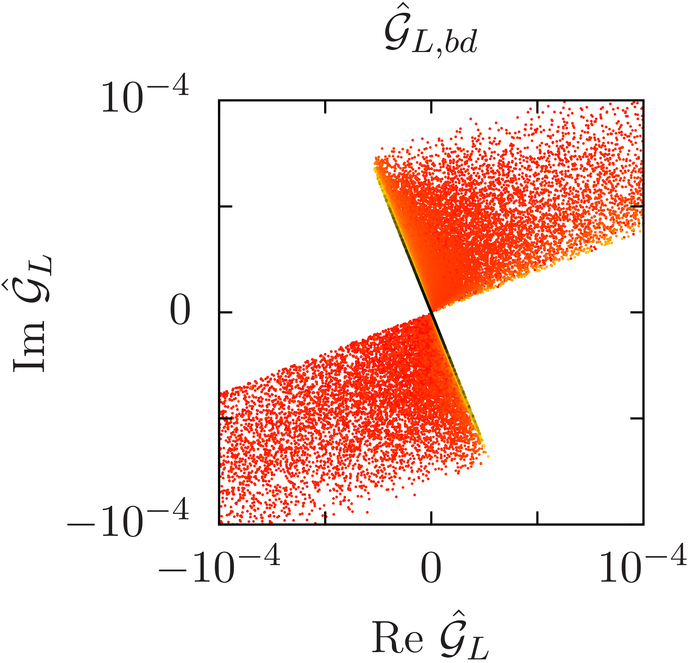
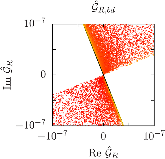
where the indices d๐‘‘d and s๐‘ s stand for the external quarks d๐‘‘d and s๐‘ s, while the index m๐‘šm refers to the A^msuperscript^๐ด๐‘š\hat{A}^{m} gauge boson mass-eigenstate. The corresponding expressions for the Bdsubscript๐ต๐‘‘B_{d} (Bssubscript๐ต๐‘ B_{s}) system are easily derived from the previous ones by substituting dโ€‹s๐‘‘๐‘ ds with dโ€‹b๐‘‘๐‘db (sโ€‹b๐‘ ๐‘sb) in the indices of the couplings. The explicit expression for the couplings (๐’ข^L,Rd)iโ€‹j,msubscriptsubscriptsuperscript^๐’ข๐‘‘๐ฟ๐‘…๐‘–๐‘—๐‘š\left(\hat{\cal G}^{d}_{L,R}\right)_{ij,m} are given in App.ย A.2.

3.4 Properties

We note a few properties:

  • -

    Focussing on eqs.ย (3.6)โ€“(3.8) and the corresponding expressions in the Bd,ssubscript๐ต๐‘‘๐‘ B_{d,s} systems, for a fixed ฮปiโ€‹ฮปjsubscript๐œ†๐‘–subscript๐œ†๐‘—\lambda_{i}\lambda_{j}, we have in the box-diagram contributions the combination

    โ„ฑiโ€‹jโ‰กcuLโ€‹i2โ€‹cuLโ€‹j2โ€‹Fโ€‹(xi,xj)+suLโ€‹i2โ€‹suLโ€‹j2โ€‹Fโ€‹(xiโ€ฒ,xjโ€ฒ)+cuLโ€‹i2โ€‹suLโ€‹j2โ€‹Fโ€‹(xi,xjโ€ฒ)+suLโ€‹i2โ€‹cuLโ€‹j2โ€‹Fโ€‹(xiโ€ฒ,xj).subscriptโ„ฑ๐‘–๐‘—subscriptsuperscript๐‘2subscript๐‘ข๐ฟ๐‘–subscriptsuperscript๐‘2subscript๐‘ข๐ฟ๐‘—๐นsubscript๐‘ฅ๐‘–subscript๐‘ฅ๐‘—subscriptsuperscript๐‘ 2subscript๐‘ข๐ฟ๐‘–subscriptsuperscript๐‘ 2subscript๐‘ข๐ฟ๐‘—๐นsubscriptsuperscript๐‘ฅโ€ฒ๐‘–subscriptsuperscript๐‘ฅโ€ฒ๐‘—subscriptsuperscript๐‘2subscript๐‘ข๐ฟ๐‘–subscriptsuperscript๐‘ 2subscript๐‘ข๐ฟ๐‘—๐นsubscript๐‘ฅ๐‘–subscriptsuperscript๐‘ฅโ€ฒ๐‘—subscriptsuperscript๐‘ 2subscript๐‘ข๐ฟ๐‘–subscriptsuperscript๐‘2subscript๐‘ข๐ฟ๐‘—๐นsubscriptsuperscript๐‘ฅโ€ฒ๐‘–subscript๐‘ฅ๐‘—{\cal F}_{ij}\equiv c^{2}_{u_{Li}}c^{2}_{u_{Lj}}F(x_{i},x_{j})+s^{2}_{u_{Li}}s^{2}_{u_{Lj}}F(x^{\prime}_{i},x^{\prime}_{j})+c^{2}_{u_{Li}}s^{2}_{u_{Lj}}F(x_{i},x^{\prime}_{j})+s^{2}_{u_{Li}}c^{2}_{u_{Lj}}F(x^{\prime}_{i},x_{j}). (3.15)

    If all fermion masses were degenerate, this combination would be independent of i,j๐‘–๐‘—i,j and the unitarity of the matrix V๐‘‰V would assure the vanishing of FCNC currents. This is precisely what one expects from the GIM mechanism.

  • -

    It is possible to arrange the function โ„ฑโ„ฑ{\cal F} in order to match with the usual notation: for the K๐พK system we write

    S0โ€‹(xt)subscript๐‘†0subscript๐‘ฅ๐‘ก\displaystyle S_{0}(x_{t}) โŸถSt(K)โ‰ก(cdLโ€‹1โ€‹cdLโ€‹2)2โ€‹(โ„ฑ33+โ„ฑ11โˆ’2โ€‹โ„ฑ13),โŸถabsentsuperscriptsubscript๐‘†๐‘ก๐พsuperscriptsubscript๐‘subscript๐‘‘๐ฟ1subscript๐‘subscript๐‘‘๐ฟ22subscriptโ„ฑ33subscriptโ„ฑ112subscriptโ„ฑ13\displaystyle\longrightarrow S_{t}^{(K)}\equiv(c_{d_{L1}}\,c_{d_{L2}})^{2}\left({\cal F}_{33}+{\cal F}_{11}-2{\cal F}_{13}\right)\,, (3.16)
    S0โ€‹(xc)subscript๐‘†0subscript๐‘ฅ๐‘\displaystyle S_{0}(x_{c}) โŸถSc(K)โ‰ก(cdLโ€‹1โ€‹cdLโ€‹2)2โ€‹(โ„ฑ22+โ„ฑ11โˆ’2โ€‹โ„ฑ12),โŸถabsentsuperscriptsubscript๐‘†๐‘๐พsuperscriptsubscript๐‘subscript๐‘‘๐ฟ1subscript๐‘subscript๐‘‘๐ฟ22subscriptโ„ฑ22subscriptโ„ฑ112subscriptโ„ฑ12\displaystyle\longrightarrow S_{c}^{(K)}\equiv(c_{d_{L1}}\,c_{d_{L2}})^{2}\left({\cal F}_{22}+{\cal F}_{11}-2{\cal F}_{12}\right)\,,
    S0โ€‹(xc,xt)subscript๐‘†0subscript๐‘ฅ๐‘subscript๐‘ฅ๐‘ก\displaystyle S_{0}(x_{c},x_{t}) โŸถScโ€‹t(K)โ‰ก(cdLโ€‹1โ€‹cdLโ€‹2)2โ€‹(โ„ฑ23+โ„ฑ11โˆ’โ„ฑ13โˆ’โ„ฑ12).โŸถabsentsuperscriptsubscript๐‘†๐‘๐‘ก๐พsuperscriptsubscript๐‘subscript๐‘‘๐ฟ1subscript๐‘subscript๐‘‘๐ฟ22subscriptโ„ฑ23subscriptโ„ฑ11subscriptโ„ฑ13subscriptโ„ฑ12\displaystyle\longrightarrow S_{ct}^{(K)}\equiv(c_{d_{L1}}\,c_{d_{L2}})^{2}\left({\cal F}_{23}+{\cal F}_{11}-{\cal F}_{13}-{\cal F}_{12}\right)\,.

    For the Bqsubscript๐ต๐‘žB_{q} systems we define similar functions Si(Bq)superscriptsubscript๐‘†๐‘–subscript๐ต๐‘žS_{i}^{(B_{q})} that can be simply derived from the previous ones by substituting cdLโ€‹1โ€‹cdLโ€‹2subscript๐‘subscript๐‘‘๐ฟ1subscript๐‘subscript๐‘‘๐ฟ2c_{d_{L1}}\,c_{d_{L2}} with cdLโ€‹1โ€‹cdLโ€‹3subscript๐‘subscript๐‘‘๐ฟ1subscript๐‘subscript๐‘‘๐ฟ3c_{d_{L1}}\,c_{d_{L3}} (cdLโ€‹2โ€‹cdLโ€‹3subscript๐‘subscript๐‘‘๐ฟ2subscript๐‘subscript๐‘‘๐ฟ3c_{d_{L2}}\,c_{d_{L3}}) in the case of q=d๐‘ž๐‘‘q=d (q=s๐‘ž๐‘ q=s). In particular the combination of the โ„ฑiโ€‹jsubscriptโ„ฑ๐‘–๐‘—{\cal F}_{ij} factors are universal. In order to recover the S0subscript๐‘†0S_{0} functions from the Si(M)subscriptsuperscript๐‘†๐‘€๐‘–S^{(M)}_{i} expressions it is necessary to take the limit in which all the cosines are equal to 111 and all the sines are zero.

  • -

    The appearance of cisubscript๐‘๐‘–c_{i} and sjsubscript๐‘ ๐‘—s_{j} factors introduces in general new flavour dependence, implying violation of certain MFV relations even in the absence of new CP-violating phases.

  • -

    There are no purely new CP-violating phases in this model, but the CP-odd phase of the CKM matrix induces sizeable new effects through new contributions to the mixing induced CP-asymmetries Sฯˆโ€‹KSsubscript๐‘†๐œ“subscript๐พ๐‘†S_{\psi K_{S}} and Sฯˆโ€‹ฯ•subscript๐‘†๐œ“italic-ฯ•S_{\psi\phi}, in the Bd0โˆ’Bยฏdsuperscriptsubscript๐ต๐‘‘0subscriptยฏ๐ต๐‘‘B_{d}^{0}-\bar{B}_{d} and the Bs0โˆ’Bยฏs0superscriptsubscript๐ต๐‘ 0superscriptsubscriptยฏ๐ต๐‘ 0B_{s}^{0}-\bar{B}_{s}^{0} systems, respectively. Moreover, similarly to the mass differences ฮ”โ€‹MBd,sฮ”subscript๐‘€subscript๐ต๐‘‘๐‘ \Delta M_{B_{d,s}}, new flavour-violating contributions affect the parameter ฮตKsubscript๐œ€๐พ\varepsilon_{K} and there are correlations between the new physics contributions to all these observables as we shall see below.

  • -

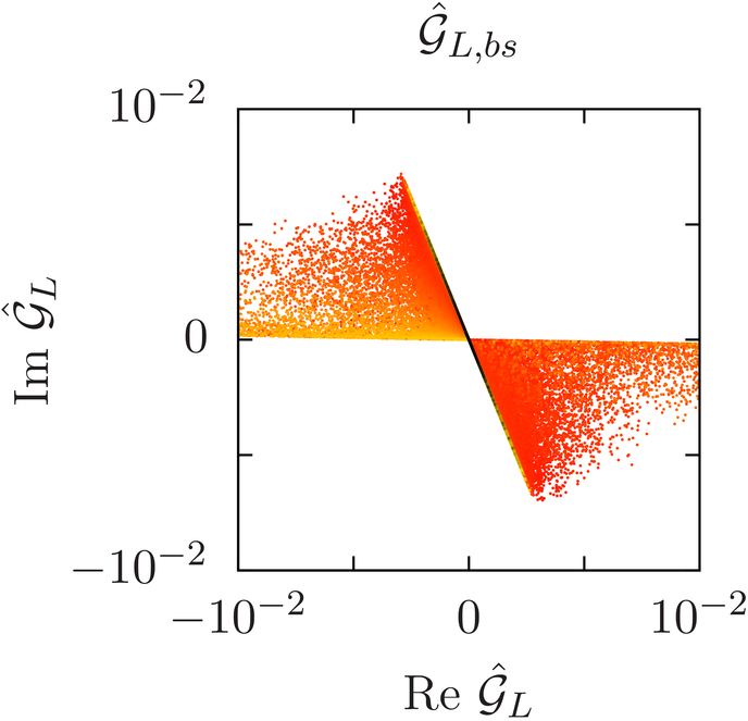
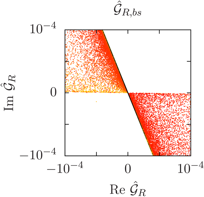
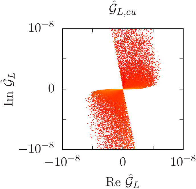
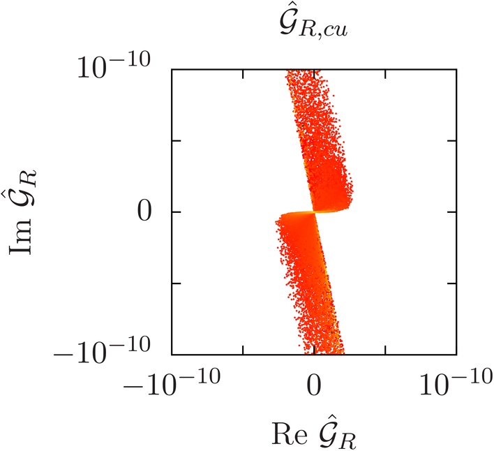
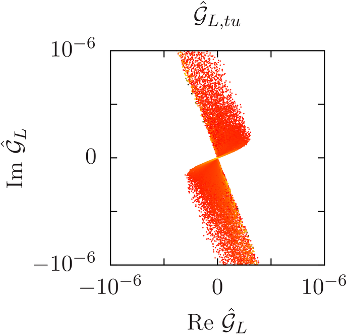
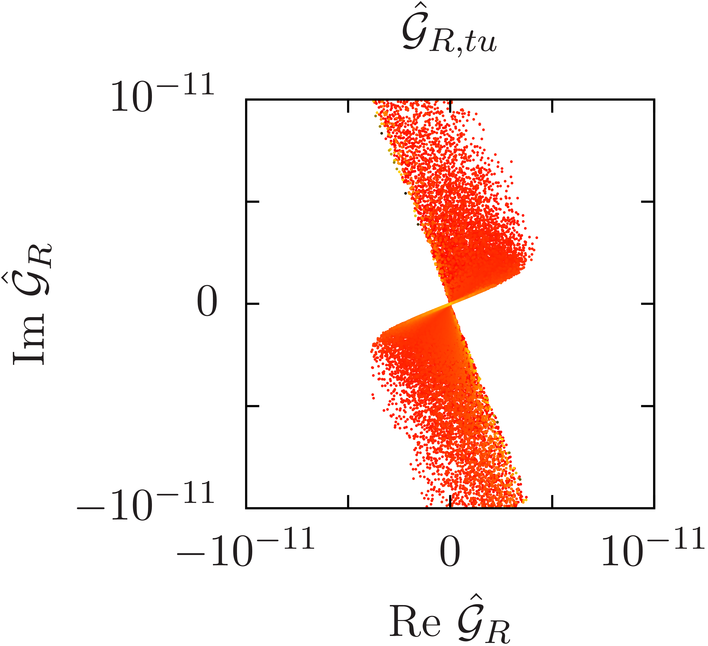
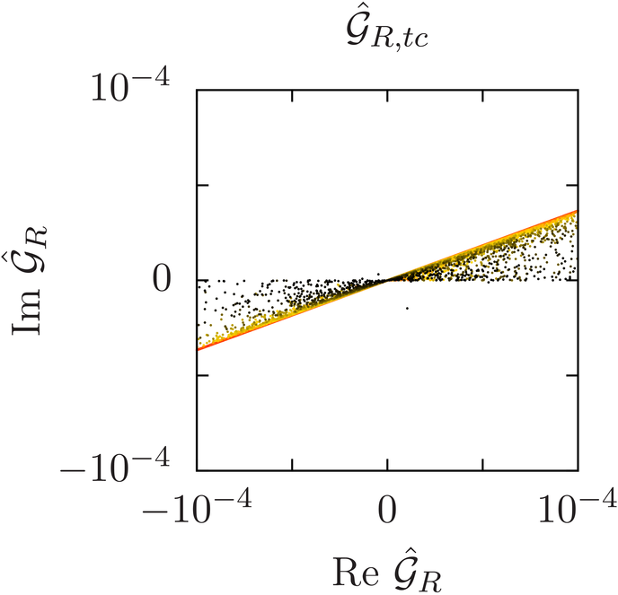
    The heavy flavour gauge bosons show flavour-violating couplings that can be strongly hierarchical: looking at the largest values of these couplings we find

    (๐’ข^L,Rd)sโ€‹bโ‰ซ(๐’ข^L,Rd)dโ€‹bโ‰ซ(๐’ข^L,Rd)dโ€‹s,(๐’ข^L,Ru)cโ€‹tโ‰ซ(๐’ข^L,Ru)uโ€‹tโ‰ซ(๐’ข^L,Ru)uโ€‹c.formulae-sequencemuch-greater-thansubscriptsubscriptsuperscript^๐’ข๐‘‘๐ฟ๐‘…๐‘ ๐‘subscriptsubscriptsuperscript^๐’ข๐‘‘๐ฟ๐‘…๐‘‘๐‘much-greater-thansubscriptsubscriptsuperscript^๐’ข๐‘‘๐ฟ๐‘…๐‘‘๐‘ much-greater-thansubscriptsubscriptsuperscript^๐’ข๐‘ข๐ฟ๐‘…๐‘๐‘กsubscriptsubscriptsuperscript^๐’ข๐‘ข๐ฟ๐‘…๐‘ข๐‘กmuch-greater-thansubscriptsubscriptsuperscript^๐’ข๐‘ข๐ฟ๐‘…๐‘ข๐‘\left(\hat{\cal G}^{d}_{L,R}\right)_{sb}\gg\left(\hat{\cal G}^{d}_{L,R}\right)_{db}\gg\left(\hat{\cal G}^{d}_{L,R}\right)_{ds}\,,\quad\quad\left(\hat{\cal G}^{u}_{L,R}\right)_{ct}\gg\left(\hat{\cal G}^{u}_{L,R}\right)_{ut}\gg\left(\hat{\cal G}^{u}_{L,R}\right)_{uc}\,. (3.17)

    An example is presented in App.ย A.2 for the lightest gauge boson. This hierarchy is due to both the mixings among SM and exotic quarks and the sequential breaking of the flavour symmetry encoded in the flavon VEVs, as seen from Eqs.ย (2.16), (A.3) and (A.4).

3.5 QCD Corrections and Hadronic Matrix Elements

The complete analysis requires the inclusion of the renormalisation group QCD evolution from the high scales, at which the initial effective Hamiltonians given above are constructed, down to low energy scales, at which the hadronic matrix elements are evaluated by lattice methods. A complication arises in the model in question as several rather different high scales are involved, such as the masses of the W๐‘ŠW-boson MWsubscript๐‘€๐‘ŠM_{W}, the masses of the neutral gauge bosons M^Amsubscript^๐‘€superscript๐ด๐‘š\hat{M}_{A^{m}} and the masses of heavy quarks mqโ€ฒโฃisubscript๐‘šsuperscript๐‘žโ€ฒ๐‘–m_{q^{\prime i}}.

Before accounting for this problem we recall a very efficient method for the inclusion of all these QCD effects in the presence of a single high scale, which we denote by ฮผHsubscript๐œ‡๐ป\mu_{H}. Instead of evaluating the hadronic matrix elements at the low-energy scale, we can evaluate them at ฮผHsubscript๐œ‡๐ป\mu_{H}, corresponding to the scale at which heavy particles are integrated out. The amplitude for Mโˆ’Mยฏ๐‘€ยฏ๐‘€M-\bar{M} mixing (M=K0,Bd0,Bs0๐‘€superscript๐พ0subscriptsuperscript๐ต0๐‘‘subscriptsuperscript๐ต0๐‘ M=K^{0},B^{0}_{d},B^{0}_{s}) at the scale ฮผHsubscript๐œ‡๐ป\mu_{H} is then simply given by

๐’œโ€‹(Mโ†’Mยฏ)=GF2โ€‹MW24โ€‹ฯ€2โ€‹โˆ‘i,aCiaโ€‹(ฮผH)โ€‹โŸจMยฏ|Qiaโ€‹(ฮผH)|MโŸฉ,๐’œโ†’๐‘€ยฏ๐‘€superscriptsubscript๐บ๐น2subscriptsuperscript๐‘€2๐‘Š4superscript๐œ‹2subscript๐‘–๐‘Žsubscriptsuperscript๐ถ๐‘Ž๐‘–subscript๐œ‡๐ปquantum-operator-productยฏ๐‘€subscriptsuperscript๐‘„๐‘Ž๐‘–subscript๐œ‡๐ป๐‘€{\cal A}(M\to\bar{M})=\dfrac{G_{F}^{2}\,M^{2}_{W}}{4\pi^{2}}\sum_{i,a}C^{a}_{i}(\mu_{H})\langle\bar{M}|Q^{a}_{i}(\mu_{H})|M\rangle\,, (3.18)

where the sum runs over all the operators listed in eq.ย (3.2). The matrix element for Mโˆ’Mยฏ๐‘€ยฏ๐‘€M-\bar{M} mixing is given by

โŸจMยฏ|Qiaโ€‹(ฮผH)|MโŸฉ=23โ€‹mM2โ€‹FM2โ€‹Piaโ€‹(M),quantum-operator-productยฏ๐‘€superscriptsubscript๐‘„๐‘–๐‘Žsubscript๐œ‡๐ป๐‘€23superscriptsubscript๐‘š๐‘€2superscriptsubscript๐น๐‘€2superscriptsubscript๐‘ƒ๐‘–๐‘Ž๐‘€\langle\bar{M}|Q_{i}^{a}(\mu_{H})|M\rangle=\dfrac{2}{3}\,m_{M}^{2}\,F_{M}^{2}\,P_{i}^{a}(M), (3.19)

where the coefficients Piaโ€‹(M)superscriptsubscript๐‘ƒ๐‘–๐‘Ž๐‘€P_{i}^{a}(M) collect compactly all RG effects from scales below ฮผHsubscript๐œ‡๐ป\mu_{H} as well as hadronic matrix elements obtained by lattice methods at low energy scales. Analytic formulae for all these coefficients, Piaโ€‹(Bq)superscriptsubscript๐‘ƒ๐‘–๐‘Žsubscript๐ต๐‘žP_{i}^{a}(B_{q}) and Piaโ€‹(K)superscriptsubscript๐‘ƒ๐‘–๐‘Ž๐พP_{i}^{a}(K), are given in Ref.ย [19], while the corresponding numerical values will be given below for some interesting values of ฮผHsubscript๐œ‡๐ป\mu_{H}.

The question then is how to generalise this method to the case at hand which involves several rather different high scales. There are three types of contributions for which the relevant high energy scales attributed to the coefficients quoted above will differ from each other:

  1. 1.

    The SM box-diagrams involving W๐‘ŠW-bosons and the SM quarks. Here the scale is chosen to be ฮผt=๐’ชโ€‹(mt)subscript๐œ‡๐‘ก๐’ชsubscript๐‘š๐‘ก\mu_{t}={\cal O}(m_{t}).

  2. 2.

    Tree-level diagrams mediated by neutral heavy gauge bosons, A^msuperscript^๐ด๐‘š\hat{A}^{m}. Since we are taking into consideration the contributions from all such gauge bosons, we shall take as the initial scale for the RG evolution in each case exactly the mass of the involved gauge boson.

  3. 3.

    The only problematic case at first sight are the contributions from box-diagrams that involve simultaneously heavy and light particles. Here the correct procedure would be to integrate out first the heavy fermions and construct an effective field theory not involving them as dynamical degrees of freedom. However, as the only relevant contribution comes from the lightest exotic fermion222This is strictly true only for the Bqsubscript๐ต๐‘žB_{q} systems, because in the K๐พK system due to the CKM suppressions, the contribution from cโ€ฒsuperscript๐‘โ€ฒc^{\prime} may be non-negligible, as accounted for in our numerical analysis. Still, the most relevant contribution comes from tโ€ฒsuperscript๐‘กโ€ฒt^{\prime}., that is tโ€ฒsuperscript๐‘กโ€ฒt^{\prime}, whose mass is relatively close to mtsubscript๐‘š๐‘กm_{t}, we can also here set the matching scale to be ฮผtsubscript๐œ‡๐‘ก\mu_{t}. As the dominant effects from RG evolution, included here, come from scales below MWsubscript๐‘€๐‘ŠM_{W}, this procedure should sufficiently well approximate the exact one.

Having the initial conditions for Wilson coefficients at a given high scale ฮผHsubscript๐œ‡๐ป\mu_{H} and provided also the corresponding hadronic matrix elements at this scale are known, we can calculate the relevant Mโˆ’Mยฏ๐‘€ยฏ๐‘€M-\bar{M} amplitude by means of eq.ย (3.18). As seen in eq.ย (3.19) these matrix elements are directly given in terms of the parameters Piaโ€‹(K)superscriptsubscript๐‘ƒ๐‘–๐‘Ž๐พP_{i}^{a}(K), Piaโ€‹(Bd)superscriptsubscript๐‘ƒ๐‘–๐‘Žsubscript๐ต๐‘‘P_{i}^{a}(B_{d}) and Piaโ€‹(Bs)superscriptsubscript๐‘ƒ๐‘–๐‘Žsubscript๐ต๐‘ P_{i}^{a}(B_{s}) for which explicit expressions in terms of RG QCD factors and the non-perturbative parameters Biaโ€‹(ฮผL)superscriptsubscript๐ต๐‘–๐‘Žsubscript๐œ‡๐ฟB_{i}^{a}(\mu_{L}) are given in eqs.ย (7.28)โ€“(7.34) of Ref.ย [19]: the ฮผLsubscript๐œ‡๐ฟ\mu_{L} denotes the low energy scale and it takes the value 2โ€‹GeV2GeV2\,{\rm GeV} (4.6โ€‹GeV4.6GeV4.6\,{\rm GeV}) for the K๐พK system (Bqsubscript๐ต๐‘žB_{q} systems).

The Biaโ€‹(ฮผL)superscriptsubscript๐ต๐‘–๐‘Žsubscript๐œ‡๐ฟB_{i}^{a}(\mu_{L}) parameters are subject to considerable uncertainties. Exception are the B1Vโ€‹Lโ€‹Lsuperscriptsubscript๐ต1๐‘‰๐ฟ๐ฟB_{1}^{VLL} parameters for which a significant progress has been made in the recent years by lattice simulations. In the SM analysis, the RG invariant parameters B^1Vโ€‹Lโ€‹Lsuperscriptsubscript^๐ต1๐‘‰๐ฟ๐ฟ\hat{B}_{1}^{VLL} are usually considered and denoted by B^Ksubscript^๐ต๐พ\hat{B}_{K} and B^Bqsubscript^๐ตsubscript๐ต๐‘ž\hat{B}_{B_{q}}. We report their values in tab.ย 3. For completeness we recall the values of B1Vโ€‹Lโ€‹Lsuperscriptsubscript๐ต1๐‘‰๐ฟ๐ฟB_{1}^{VLL} that we extracted from the most recent lattice simulations:

B1Vโ€‹Lโ€‹L=0.515โ€‹(14),superscriptsubscript๐ต1๐‘‰๐ฟ๐ฟ0.51514\displaystyle B_{1}^{VLL}=0.515(14)\,,\qquad\qquad for K๐พK system (3.20)
B1Vโ€‹Lโ€‹L=0.825โ€‹(72),superscriptsubscript๐ต1๐‘‰๐ฟ๐ฟ0.82572\displaystyle B_{1}^{VLL}=0.825(72)\,,\qquad\qquad for Bdsubscript๐ต๐‘‘B_{d} system
B1Vโ€‹Lโ€‹L=0.871โ€‹(39),superscriptsubscript๐ต1๐‘‰๐ฟ๐ฟ0.87139\displaystyle B_{1}^{VLL}=0.871(39)\,,\qquad\qquad forย Bsย system.forย Bsย system\displaystyle\text{for $B_{s}$ system}\,.

As these parameters are the same for VRR contributions we will combine them together with the VLL contributions in the final formula at the end of this section.

Neglecting the unknown ๐’ชโ€‹(ฮฑs)๐’ชsubscript๐›ผ๐‘ {\cal O}(\alpha_{s}) contributions to Wilson coefficients of the remaining operators at the high energy scale, our NLO RG analysis involves only the values of the coefficients P1Lโ€‹Rโ€‹(K)superscriptsubscript๐‘ƒ1๐ฟ๐‘…๐พP_{1}^{LR}(K), P1Lโ€‹Rโ€‹(Bd)superscriptsubscript๐‘ƒ1๐ฟ๐‘…subscript๐ต๐‘‘P_{1}^{LR}(B_{d}) and P1Lโ€‹Rโ€‹(Bs)superscriptsubscript๐‘ƒ1๐ฟ๐‘…subscript๐ต๐‘ P_{1}^{LR}(B_{s}) calculated at ฮผHsubscript๐œ‡๐ป\mu_{H}. We are not considering the intermediate thresholds of exotic quarks, since the smallness of ฮฑssubscript๐›ผ๐‘ \alpha_{s} and the absence of the flavour dependence in the LO anomalous dimensions of the contributing operators render the corresponding effects negligible. To obtain these values we need only the values of B1Lโ€‹Rsuperscriptsubscript๐ต1๐ฟ๐‘…B_{1}^{LR} and B2Lโ€‹Rsuperscriptsubscript๐ต2๐ฟ๐‘…B_{2}^{LR}, that we report below in the NDR scheme333These values can be found in Refs.ย [20, 21], where B1Lโ€‹Rsuperscriptsubscript๐ต1๐ฟ๐‘…B_{1}^{LR} (B2Lโ€‹Rsuperscriptsubscript๐ต2๐ฟ๐‘…B_{2}^{LR}) is called B5subscript๐ต5B_{5} (B4subscript๐ต4B_{4}). [20, 21]:

B1Lโ€‹R=0.562โ€‹(39)โ€‹(46),superscriptsubscript๐ต1๐ฟ๐‘…0.5623946\displaystyle B_{1}^{LR}=0.562(39)(46)\,,\qquad B2Lโ€‹R=0.810โ€‹(41)โ€‹(31),superscriptsubscript๐ต2๐ฟ๐‘…0.8104131\displaystyle B_{2}^{LR}=0.810(41)(31)\,,\qquad for K๐พK system (3.21)
B1Lโ€‹R=1.72(4)()โˆ’6+20,\displaystyle B_{1}^{LR}=1.72(4)({}^{+20}_{-6})\,,\qquad B2Lโ€‹R=1.15(3)()โˆ’7+5,\displaystyle B_{2}^{LR}=1.15(3)({}^{+5}_{-7})\,,\qquad for Bdsubscript๐ต๐‘‘B_{d} system
B1Lโ€‹R=1.75(3)()โˆ’6+21,\displaystyle B_{1}^{LR}=1.75(3)({}^{+21}_{-6})\,,\qquad B2Lโ€‹R=1.16(2)()โˆ’7+5,\displaystyle B_{2}^{LR}=1.16(2)({}^{+5}_{-7})\,,\qquad forย Bsย system.forย Bsย system\displaystyle\text{for $B_{s}$ system}\,.

In tab.ย 2, we show the resulting Pisubscript๐‘ƒ๐‘–P_{i} factors for some relevant values of ฮผHsubscript๐œ‡๐ป\mu_{H}.

ฮผHsubscript๐œ‡๐ป~{}\qquad\mu_{H} 500โ€‹GeV500GeV500\,{\rm GeV} 1โ€‹TeV1TeV1\,{\rm TeV} 3โ€‹TeV3TeV3\,{\rm TeV} 10โ€‹TeV10TeV10\,{\rm TeV}
P1Vโ€‹Lโ€‹Lโ€‹(ฮผH,K)superscriptsubscript๐‘ƒ1๐‘‰๐ฟ๐ฟsubscript๐œ‡๐ป๐พP_{1}^{VLL}(\mu_{H},\,K) 0.392 0.384 0.373 0.363
P1Lโ€‹Rโ€‹(ฮผH,K)superscriptsubscript๐‘ƒ1๐ฟ๐‘…subscript๐œ‡๐ป๐พP_{1}^{LR}(\mu_{H},\,K) -35.7 -39.3 -45.0 -51.4
P1Vโ€‹Lโ€‹Lโ€‹(ฮผH,Bd)superscriptsubscript๐‘ƒ1๐‘‰๐ฟ๐ฟsubscript๐œ‡๐ปsubscript๐ต๐‘‘P_{1}^{VLL}(\mu_{H},\,B_{d}) 0.675 0.662 0.643 0.624
P1Lโ€‹Rโ€‹(ฮผH,Bd)superscriptsubscript๐‘ƒ1๐ฟ๐‘…subscript๐œ‡๐ปsubscript๐ต๐‘‘P_{1}^{LR}(\mu_{H},\,B_{d}) -2.76 -2.97 -3.31 -3.69
P1Vโ€‹Lโ€‹Lโ€‹(ฮผH,Bs)superscriptsubscript๐‘ƒ1๐‘‰๐ฟ๐ฟsubscript๐œ‡๐ปsubscript๐ต๐‘ P_{1}^{VLL}(\mu_{H},\,B_{s}) 0.713 0.698 0.678 0.659
P1Lโ€‹Rโ€‹(ฮผH,Bs)superscriptsubscript๐‘ƒ1๐ฟ๐‘…subscript๐œ‡๐ปsubscript๐ต๐‘ P_{1}^{LR}(\mu_{H},\,B_{s}) -2.76 -2.97 -3.31 -3.69
Table 2: Central values of Pisubscript๐‘ƒ๐‘–P_{i} factors for ฮผH={0.5,โ€‰1,โ€‰3,โ€‰10}โ€‹TeVsubscript๐œ‡๐ป0.51310TeV\mu_{H}=\{0.5,\,1,\,3,\,10\}\,{\rm TeV}.

Notice that the LR operators, arising from integrating out the heavy flavour gauge bosons, are strongly enhanced by the RG QCD running as can be deduced from the values of the P1Lโ€‹Rsuperscriptsubscript๐‘ƒ1๐ฟ๐‘…P_{1}^{LR} factors. A priori, such contributions could be very important.

3.6 Final Formulae for ๐šซโ€‹๐‘ญ=๐Ÿ๐šซ๐‘ญ2\Delta F=2 Observables

We collect here the formulae we shall use in our numerical analysis. The mixing amplitude M12isubscriptsuperscript๐‘€๐‘–12M^{i}_{12} (i=K,d,s)๐‘–๐พ๐‘‘๐‘ (i=K,d,s) is related to the relevant effective Hamiltonian through

2โ€‹mKโ€‹(M12K)โˆ—=โŸจKยฏ0|โ„‹ย effฮ”โ€‹S=2|K0โŸฉ,2โ€‹mBqโ€‹(M12q)โˆ—=โŸจBยฏq0|โ„‹ย effฮ”โ€‹B=2|Bq0โŸฉformulae-sequence2subscript๐‘š๐พsuperscriptsuperscriptsubscript๐‘€12๐พโˆ—quantum-operator-productsuperscriptยฏ๐พ0superscriptsubscriptโ„‹ย effฮ”๐‘†2superscript๐พ02subscript๐‘šsubscript๐ต๐‘žsuperscriptsuperscriptsubscript๐‘€12๐‘žโˆ—quantum-operator-productsuperscriptsubscriptยฏ๐ต๐‘ž0superscriptsubscriptโ„‹ย effฮ”๐ต2superscriptsubscript๐ต๐‘ž02\,m_{K}\left(M_{12}^{K}\right)^{\ast}=\langle\bar{K}^{0}|{\cal H}_{\text{ eff}}^{\Delta S=2}|K^{0}\rangle\,,\qquad\qquad 2\,m_{B_{q}}\left(M_{12}^{q}\right)^{\ast}=\langle\bar{B}_{q}^{0}|{\cal H}_{\text{ eff}}^{\Delta B=2}|B_{q}^{0}\rangle (3.22)

with q=d,s๐‘ž๐‘‘๐‘ q=d,s. The KLโˆ’KSsubscript๐พ๐ฟsubscript๐พ๐‘†K_{L}-K_{S} mass difference and the CP-violating parameter ฮตKsubscript๐œ€๐พ\varepsilon_{K} are then given by

ฮ”โ€‹MK=2โ€‹Reโก(M12K),ฮตK=ฮบฯตโ€‹eiโ€‹ฯ†ฯต2โ€‹(ฮ”โ€‹MK)expโ€‹Imโก(M12K),formulae-sequenceฮ”subscript๐‘€๐พ2Resuperscriptsubscript๐‘€12๐พsubscript๐œ€๐พsubscript๐œ…italic-ฯตsuperscript๐‘’๐‘–subscript๐œ‘italic-ฯต2subscriptฮ”subscript๐‘€๐พexpImsuperscriptsubscript๐‘€12๐พ\Delta M_{K}=2\operatorname{Re}\left(M_{12}^{K}\right)\,,\qquad\qquad\varepsilon_{K}=\dfrac{\kappa_{\epsilon}\,e^{i\,\varphi_{\epsilon}}}{\sqrt{2}(\Delta M_{K})_{\text{exp}}}\operatorname{Im}\left(M_{12}^{K}\right)\,, (3.23)

where ฯ†ฯต=(43.51ยฑ0.05)โˆ˜subscript๐œ‘italic-ฯตsuperscriptplus-or-minus43.510.05\varphi_{\epsilon}=(43.51\pm 0.05)^{\circ} and ฮบฯต=0.923ยฑ0.006subscript๐œ…italic-ฯตplus-or-minus0.9230.006\kappa_{\epsilon}=0.923\pm 0.006 takes into account that ฯ†ฯตโ‰ ฯ€/4subscript๐œ‘italic-ฯต๐œ‹4\varphi_{\epsilon}\neq\pi/4 and includes long distance effect in Imโกฮ“12Imsubscriptฮ“12\operatorname{Im}\Gamma_{12} [22] 444This value has been confirmed by lattice and presented with a smaller error in Ref.ย [23]. and ImโกM12Imsubscript๐‘€12\operatorname{Im}M_{12} [24]. The mixing amplitude entering the previous expressions can be decomposed into two parts, one containing the Lโ€‹L๐ฟ๐ฟLL and Rโ€‹R๐‘…๐‘…RR contributions and the second only the Lโ€‹R๐ฟ๐‘…LR ones:

M12K=(M12K)1+(M12K)2,subscriptsuperscript๐‘€๐พ12subscriptsubscriptsuperscript๐‘€๐พ121subscriptsubscriptsuperscript๐‘€๐พ122M^{K}_{12}=(M^{K}_{12})_{1}+(M^{K}_{12})_{2}, (3.24)

where

(M12K)1=GF2โ€‹MW212โ€‹ฯ€2FK2mK[B^Kโ€‹ฮท1โ€‹ฮป22โ€‹(K)โ€‹Sc(K)+B^Kโ€‹ฮท2โ€‹ฮป32โ€‹(K)โ€‹St(K)++2โ€‹B^Kโ€‹ฮท3โ€‹ฮป2โ€‹(K)โ€‹ฮป3โ€‹(K)โ€‹Scโ€‹t(K)++P1Vโ€‹Lโ€‹L(ฮผH,K)(ฮ”A(K)C1Vโ€‹Lโ€‹L(ฮผH)+ฮ”A(K)CVโ€‹Rโ€‹R(ฮผH))]โˆ—,subscriptsuperscriptsubscript๐‘€12๐พ1superscriptsubscript๐บ๐น2superscriptsubscript๐‘€๐‘Š212superscript๐œ‹2superscriptsubscript๐น๐พ2subscript๐‘š๐พsuperscriptdelimited-[]subscript^๐ต๐พsubscript๐œ‚1subscriptsuperscript๐œ†22๐พsubscriptsuperscript๐‘†๐พ๐‘subscript^๐ต๐พsubscript๐œ‚2subscriptsuperscript๐œ†23๐พsubscriptsuperscript๐‘†๐พ๐‘ก2subscript^๐ต๐พsubscript๐œ‚3subscript๐œ†2๐พsubscript๐œ†3๐พsuperscriptsubscript๐‘†๐‘๐‘ก๐พsuperscriptsubscript๐‘ƒ1๐‘‰๐ฟ๐ฟsubscript๐œ‡๐ป๐พsubscriptsuperscriptฮ”๐พ๐ดsuperscriptsubscript๐ถ1๐‘‰๐ฟ๐ฟsubscript๐œ‡๐ปsubscriptsuperscriptฮ”๐พ๐ดsuperscript๐ถ๐‘‰๐‘…๐‘…subscript๐œ‡๐ป\displaystyle\begin{split}(M_{12}^{K})_{1}=\dfrac{G_{F}^{2}\,M_{W}^{2}}{12\pi^{2}}\,F_{K}^{2}\,m_{K}\Big{[}&\hat{B}_{K}\,\eta_{1}\,\lambda^{2}_{2}(K)\,S^{(K)}_{c}+\hat{B}_{K}\,\eta_{2}\,\lambda^{2}_{3}(K)\,S^{(K)}_{t}+\\ &+2\,\hat{B}_{K}\,\eta_{3}\,\lambda_{2}(K)\,\lambda_{3}(K)\,S_{ct}^{(K)}+\\ &+P_{1}^{VLL}(\mu_{H},K)\,\left(\Delta^{(K)}_{A}\,C_{1}^{VLL}(\mu_{H})+\Delta^{(K)}_{A}\,C^{VRR}(\mu_{H})\right)\,\Big{]}^{*}\,,\end{split} (3.25)
(M12K)2=GF2โ€‹MW212โ€‹ฯ€2โ€‹FK2โ€‹mKโ€‹P1Lโ€‹Rโ€‹(ฮผH,K)โ€‹ฮ”A(K)โ€‹C1Lโ€‹Rโฃโˆ—โ€‹(ฮผH).subscriptsuperscriptsubscript๐‘€12๐พ2superscriptsubscript๐บ๐น2superscriptsubscript๐‘€๐‘Š212superscript๐œ‹2superscriptsubscript๐น๐พ2subscript๐‘š๐พsuperscriptsubscript๐‘ƒ1๐ฟ๐‘…subscript๐œ‡๐ป๐พsubscriptsuperscriptฮ”๐พ๐ดsuperscriptsubscript๐ถ1๐ฟ๐‘…subscript๐œ‡๐ป\displaystyle(M_{12}^{K})_{2}=\dfrac{G_{F}^{2}\,M_{W}^{2}}{12\pi^{2}}\,F_{K}^{2}\,m_{K}\,P_{1}^{LR}(\mu_{H},K)\,\Delta^{(K)}_{A}\,C_{1}^{LR*}(\mu_{H})\,.

Analogously, for the the Bd,s0โˆ’Bยฏd,s0superscriptsubscript๐ต๐‘‘๐‘ 0superscriptsubscriptยฏ๐ต๐‘‘๐‘ 0B_{d,s}^{0}-\bar{B}_{d,s}^{0} systems the two parts of the mixing amplitude are given by:

(M12q)1=GF2โ€‹MW212โ€‹ฯ€2FBq2mBq[ฮทBโ€‹B^Bqโ€‹ฮป32โ€‹(Bq)โ€‹St(Bq)++P1Vโ€‹Lโ€‹L(ฮผH,Bq)(ฮ”A(Bq)C1Vโ€‹Lโ€‹L(ฮผH)+ฮ”A(Bq)CVโ€‹Rโ€‹R(ฮผH))]โˆ—,subscriptsuperscriptsubscript๐‘€12๐‘ž1superscriptsubscript๐บ๐น2subscriptsuperscript๐‘€2๐‘Š12superscript๐œ‹2subscriptsuperscript๐น2subscript๐ต๐‘žsubscript๐‘šsubscript๐ต๐‘žsuperscriptdelimited-[]subscript๐œ‚๐ตsubscript^๐ตsubscript๐ต๐‘žsubscriptsuperscript๐œ†23subscript๐ต๐‘žsuperscriptsubscript๐‘†๐‘กsubscript๐ต๐‘žsuperscriptsubscript๐‘ƒ1๐‘‰๐ฟ๐ฟsubscript๐œ‡๐ปsubscript๐ต๐‘žsubscriptsuperscriptฮ”subscript๐ต๐‘ž๐ดsuperscriptsubscript๐ถ1๐‘‰๐ฟ๐ฟsubscript๐œ‡๐ปsubscriptsuperscriptฮ”subscript๐ต๐‘ž๐ดsuperscript๐ถ๐‘‰๐‘…๐‘…subscript๐œ‡๐ป\displaystyle\begin{split}(M_{12}^{q})_{1}=\dfrac{G_{F}^{2}\,M^{2}_{W}}{12\pi^{2}}\,F^{2}_{B_{q}}\,m_{B_{q}}\,\Big{[}&\eta_{B}\,\hat{B}_{B_{q}}\,\lambda^{2}_{3}(B_{q})\,\,S_{t}^{(B_{q})}+\\ &+P_{1}^{VLL}(\mu_{H},B_{q})\,\left(\Delta^{(B_{q})}_{A}C_{1}^{VLL}(\mu_{H})+\Delta^{(B_{q})}_{A}C^{VRR}(\mu_{H})\right)\Big{]}^{*}\,,\end{split} (3.26)
(M12q)2=GF2โ€‹MW212โ€‹ฯ€2โ€‹FBq2โ€‹mBqโ€‹P1Lโ€‹Rโ€‹(ฮผH,Bq)โ€‹ฮ”A(Bq)โ€‹C1Lโ€‹Rโฃโˆ—โ€‹(ฮผH).subscriptsuperscriptsubscript๐‘€12๐‘ž2superscriptsubscript๐บ๐น2subscriptsuperscript๐‘€2๐‘Š12superscript๐œ‹2subscriptsuperscript๐น2subscript๐ต๐‘žsubscript๐‘šsubscript๐ต๐‘žsuperscriptsubscript๐‘ƒ1๐ฟ๐‘…subscript๐œ‡๐ปsubscript๐ต๐‘žsubscriptsuperscriptฮ”subscript๐ต๐‘ž๐ดsuperscriptsubscript๐ถ1๐ฟ๐‘…subscript๐œ‡๐ป\displaystyle(M_{12}^{q})_{2}=\frac{G_{F}^{2}\,M^{2}_{W}}{12\pi^{2}}\,F^{2}_{B_{q}}\,m_{B_{q}}\,P_{1}^{LR}(\mu_{H},B_{q})\,\Delta^{(B_{q})}_{A}C_{1}^{LR*}(\mu_{H})\,.

Here ฮท1,2,3,Bsubscript๐œ‚123๐ต\eta_{1,2,3,B} are known SM QCD corrections given in tab.ย 3 and Piaโ€‹(ฮผH,M)superscriptsubscript๐‘ƒ๐‘–๐‘Žsubscript๐œ‡๐ป๐‘€P_{i}^{a}(\mu_{H},M) describe the QCD evolution from ฮผHsubscript๐œ‡๐ป\mu_{H} down to ฮผLsubscript๐œ‡๐ฟ\mu_{L} for the considered system. For the Bqsubscript๐ต๐‘žB_{q} systems, it is useful to rearrange the definition of the mixing amplitude M12qsuperscriptsubscript๐‘€12๐‘žM_{12}^{q} as follows [25]

M12q=(M12q)SMโ€‹CBqโ€‹e2โ€‹iโ€‹ฯ†Bq,superscriptsubscript๐‘€12๐‘žsubscriptsuperscriptsubscript๐‘€12๐‘žSMsubscript๐ถsubscript๐ต๐‘žsuperscript๐‘’2๐‘–subscript๐œ‘subscript๐ต๐‘žM_{12}^{q}=\left(M_{12}^{q}\right)_{\text{SM}}C_{B_{q}}e^{2\,i\,\varphi_{B_{q}}}\,, (3.27)

where CBd,ssubscript๐ถsubscript๐ต๐‘‘๐‘ C_{B_{d,s}} and ฯ†Bd,ssubscript๐œ‘subscript๐ต๐‘‘๐‘ \varphi_{B_{d,s}} account for deviations from the SM contributions. Therefore, the mass differences turn out to be

ฮ”โ€‹MBq=2โ€‹|M12q|=(ฮ”โ€‹MBq)SMโ€‹CBq(q=d,s),formulae-sequenceฮ”subscript๐‘€subscript๐ต๐‘ž2superscriptsubscript๐‘€12๐‘žsubscriptฮ”subscript๐‘€subscript๐ต๐‘žSMsubscript๐ถsubscript๐ต๐‘ž๐‘ž๐‘‘๐‘ \Delta M_{B_{q}}=2\left|M_{12}^{q}\right|=(\Delta M_{B_{q}})_{\text{SM}}C_{B_{q}}\qquad(q=d,s)\,, (3.28)

where

(M12d)SM=|(M12d)SM|e2โ€‹iโ€‹ฮฒ,(M12s)SM=|(M12s)SM|e2โ€‹iโ€‹ฮฒs.\bigl{(}M_{12}^{d}\bigr{)}_{\text{SM}}=\bigl{|}\bigl{(}M_{12}^{d}\bigr{)}_{\text{SM}}\bigr{|}e^{2\,i\,\beta}\,,\qquad\qquad\bigl{(}M_{12}^{s}\bigr{)}_{\text{SM}}=\bigl{|}\bigl{(}M_{12}^{s}\bigr{)}_{\text{SM}}\bigr{|}e^{2\,i\,\beta_{s}}\,. (3.29)

Here the phases ฮฒโ‰ˆ22โˆ˜๐›ฝsuperscript22\beta\approx 22^{\circ} and ฮฒsโ‰ƒโˆ’1โˆ˜similar-to-or-equalssubscript๐›ฝ๐‘ superscript1\beta_{s}\simeq-1^{\circ} are defined through

Vtโ€‹dSโ€‹M=|Vtโ€‹dSโ€‹M|โ€‹eโˆ’iโ€‹ฮฒandVtโ€‹sSโ€‹M=โˆ’|Vtโ€‹sSโ€‹M|โ€‹eโˆ’iโ€‹ฮฒs.formulae-sequencesubscriptsuperscript๐‘‰๐‘†๐‘€๐‘ก๐‘‘superscriptsubscript๐‘‰๐‘ก๐‘‘๐‘†๐‘€superscript๐‘’๐‘–๐›ฝandsubscriptsuperscript๐‘‰๐‘†๐‘€๐‘ก๐‘ subscriptsuperscript๐‘‰๐‘†๐‘€๐‘ก๐‘ superscript๐‘’๐‘–subscript๐›ฝ๐‘ V^{SM}_{td}=|V_{td}^{SM}|e^{-i\beta}\qquad\qquad\textrm{and}\qquad\qquad V^{SM}_{ts}=-|V^{SM}_{ts}|e^{-i\beta_{s}}\,. (3.30)

The coefficients of sinโก(ฮ”โ€‹MBdโ€‹t)ฮ”subscript๐‘€subscript๐ต๐‘‘๐‘ก\sin(\Delta M_{B_{d}}\,t) and sinโก(ฮ”โ€‹MBsโ€‹t)ฮ”subscript๐‘€subscript๐ต๐‘ ๐‘ก\sin(\Delta M_{B_{s}}\,t) in the time dependent asymmetries in Bd0โ†’ฯˆโ€‹KSโ†’superscriptsubscript๐ต๐‘‘0๐œ“subscript๐พ๐‘†B_{d}^{0}\to\psi K_{S} and Bs0โ†’ฯˆโ€‹ฯ•โ†’superscriptsubscript๐ต๐‘ 0๐œ“italic-ฯ•B_{s}^{0}\to\psi\phi are then given, respectively, by:

Sฯˆโ€‹KS=sinโก(2โ€‹ฮฒ+2โ€‹ฯ†Bd),Sฯˆโ€‹ฯ•=sinโก(2โ€‹|ฮฒs|โˆ’2โ€‹ฯ†Bs).formulae-sequencesubscript๐‘†๐œ“subscript๐พ๐‘†2๐›ฝ2subscript๐œ‘subscript๐ต๐‘‘subscript๐‘†๐œ“italic-ฯ•2subscript๐›ฝ๐‘ 2subscript๐œ‘subscript๐ต๐‘ S_{\psi K_{S}}=\sin(2\beta+2\varphi_{B_{d}})\,,\qquad\qquad S_{\psi\phi}=\sin(2|\beta_{s}|-2\varphi_{B_{s}})\,. (3.31)

Notice that in the presence of non-vanishing ฯ†Bdsubscript๐œ‘subscript๐ต๐‘‘\varphi_{B_{d}} and ฯ†Bssubscript๐œ‘subscript๐ต๐‘ \varphi_{B_{s}} these two asymmetries do not measure ฮฒ๐›ฝ\beta and ฮฒssubscript๐›ฝ๐‘ \beta_{s} but (ฮฒ+ฯ†Bd)๐›ฝsubscript๐œ‘subscript๐ต๐‘‘(\beta+\varphi_{B_{d}}) and (|ฮฒs|โˆ’ฯ†Bs)subscript๐›ฝ๐‘ subscript๐œ‘subscript๐ต๐‘ (|\beta_{s}|-\varphi_{B_{s}}), respectively.

3.7 The Ratio ๐šซโ€‹๐‘ด๐‘ฉ๐’…/๐šซโ€‹๐‘ด๐‘ฉ๐’”๐šซsubscript๐‘ดsubscript๐‘ฉ๐’…๐šซsubscript๐‘ดsubscript๐‘ฉ๐’”\Delta M_{B_{d}}/\Delta{M_{B_{s}}} and the ๐‘ฉ+โ†’๐‰+โ€‹๐‚bold-โ†’superscript๐‘ฉsuperscript๐‰๐‚B^{+}\to\tau^{+}\nu Decay

The expressions for the mass-differences recovered in the previous section are affected by large uncertainties, driven by the decay constants ๐‘ญ๐‘ฉ๐’…,๐’”subscript๐‘ญsubscript๐‘ฉ๐’…๐’”F_{B_{d,s}}. To soften the dependence of our analysis on these theoretical errors, we consider the ratio among ๐šซโ€‹๐‘ด๐‘ฉ๐’…๐šซsubscript๐‘ดsubscript๐‘ฉ๐’…\Delta M_{B_{d}} and ๐šซโ€‹๐‘ด๐‘ฉ๐’”๐šซsubscript๐‘ดsubscript๐‘ฉ๐’”\Delta M_{B_{s}}, that we call ๐‘น๐šซโ€‹๐‘ด๐‘ฉsubscript๐‘น๐šซsubscript๐‘ด๐‘ฉR_{\Delta M_{B}}, and the ratio among the branching ratio of the ๐‘ฉ+โ†’๐‰+โ€‹๐‚bold-โ†’superscript๐‘ฉsuperscript๐‰๐‚B^{+}\to\tau^{+}\nu decay and ๐šซโ€‹๐‘ด๐‘ฉ๐’…๐šซsubscript๐‘ดsubscript๐‘ฉ๐’…\Delta M_{B_{d}}, that we name ๐‘น๐‘ฉโ€‹๐‘น/๐šซโ€‹๐‘ดsubscript๐‘น๐‘ฉ๐‘น๐šซ๐‘ดR_{BR/\Delta M}.

Indeed, when considering ๐‘น๐šซโ€‹๐‘ด๐‘ฉsubscript๐‘น๐šซsubscript๐‘ด๐‘ฉR_{\Delta M_{B}}, we notice that the SM theoretical errors are encoded into the parameter ๐ƒ=1.237ยฑ0.032๐ƒplus-or-minus1.2370.032\xi=1.237\pm 0.032, that is much less affected by uncertainties with respect to the mass differences. When considering the NP effects, we obtain

๐‘น๐šซโ€‹๐‘ด๐‘ฉ=(๐šซโ€‹๐‘ด๐‘ฉ๐’…)SM(๐šซโ€‹๐‘ด๐‘ฉ๐’”)SMโ€‹๐‘ช๐‘ฉ๐’…๐‘ช๐‘ฉ๐’”.subscript๐‘น๐šซsubscript๐‘ด๐‘ฉsubscript๐šซsubscript๐‘ดsubscript๐‘ฉ๐’…SMsubscript๐šซsubscript๐‘ดsubscript๐‘ฉ๐’”SMsubscript๐‘ชsubscript๐‘ฉ๐’…subscript๐‘ชsubscript๐‘ฉ๐’”R_{\Delta M_{B}}=\dfrac{(\Delta M_{B_{d}})_{\text{SM}}}{(\Delta M_{B_{s}})_{\text{SM}}}\dfrac{C_{B_{d}}}{C_{B_{s}}}\,. (3.32)

On the other hand, in the SM, the ๐‘ฉ+โ†’๐‰+โ€‹๐‚bold-โ†’superscript๐‘ฉsuperscript๐‰๐‚B^{+}\to\tau^{+}\nu decay occurs at the tree-level through the exchange of the ๐‘พ๐‘พW-boson. Therefore, the expression for its branching ratio is only slightly modified in our model:

๐‘ฉโ€‹๐‘นโ€‹(๐‘ฉ+โ†’๐‰+โ€‹๐‚)=๐‘ฎ๐‘ญ๐Ÿโ€‹๐’Ž๐‘ฉ+โ€‹๐’Ž๐‰๐Ÿ๐Ÿ–โ€‹๐…โ€‹(๐Ÿโˆ’๐’Ž๐‰๐Ÿ๐’Ž๐‘ฉ+๐Ÿ)๐Ÿโ€‹๐‘ญ๐‘ฉ+๐Ÿโ€‹|๐’„๐’–๐‘ณโ€‹๐Ÿโ€‹๐‘ฝ๐’–โ€‹๐’ƒโ€‹๐’„๐’…๐‘ณโ€‹๐Ÿ‘|๐Ÿโ€‹๐‰๐‘ฉ+,๐‘ฉ๐‘นbold-โ†’superscript๐‘ฉsuperscript๐‰๐‚superscriptsubscript๐‘ฎ๐‘ญ2subscript๐’Žsuperscript๐‘ฉsuperscriptsubscript๐’Ž๐‰28๐…superscript1superscriptsubscript๐’Ž๐‰2subscriptsuperscript๐’Ž2superscript๐‘ฉ2subscriptsuperscript๐‘ญ2superscript๐‘ฉsuperscriptsubscript๐’„subscript๐’–๐‘ณ1subscript๐‘ฝ๐’–๐’ƒsubscript๐’„subscript๐’…๐‘ณ32subscript๐‰superscript๐‘ฉBR(B^{+}\to\tau^{+}\nu)=\dfrac{G_{F}^{2}\,m_{B^{+}}\,m_{\tau}^{2}}{8\pi}\left(1-\dfrac{m_{\tau}^{2}}{m^{2}_{B^{+}}}\right)^{2}\,F^{2}_{B^{+}}\,|c_{u_{L1}}\,V_{ub}\,c_{d_{L3}}|^{2}\,\tau_{B^{+}}\,, (3.33)

where the NP effects are represented by the cosines. Notice that heavy flavour gauge boson contributions could contribute only at the loop-level and can be safely neglected, since they compete with a tree-level process. Furthermore, in the previous expression we have assumed the SM couplings for the leptons to the ๐‘พ๐‘พW-boson: even if we are not considering the lepton sector in our analysis it is reasonable to assume that any NP modification can be safely negligible, as these couplings are strongly constrained by the SM electroweak analysis.

In the ratio ๐‘น๐‘ฉโ€‹๐‘น/๐šซโ€‹๐‘ดsubscript๐‘น๐‘ฉ๐‘น๐šซ๐‘ดR_{BR/\Delta M}, the dependence on ๐‘ญ๐‘ฉ๐’…subscript๐‘ญsubscript๐‘ฉ๐’…F_{B_{d}}, which is indeed the main source of the theoretical error on ๐šซโ€‹๐‘ด๐‘ฉ๐’…๐šซsubscript๐‘ดsubscript๐‘ฉ๐’…\Delta M_{B_{d}}, is cancelled [26, 27]:

๐‘น๐‘ฉโ€‹๐‘น/๐šซโ€‹๐‘ด=๐Ÿ‘โ€‹๐…โ€‹๐‰๐‘ฉ+๐Ÿ’โ€‹๐œผ๐‘ฉโ€‹๐‘ฉ^๐‘ฉ๐’…โ€‹๐‘บ๐ŸŽโ€‹(๐’™๐’•)โ€‹๐’„๐’–๐‘ณโ€‹๐Ÿ๐Ÿโ€‹๐’„๐’…๐‘ณโ€‹๐Ÿ‘๐Ÿ๐‘ช๐‘ฉ๐’…โ€‹๐’Ž๐‰๐Ÿ๐‘ด๐‘พ๐Ÿโ€‹|๐‘ฝ๐’–โ€‹๐’ƒ|๐Ÿ|๐‘ฝ๐’•โ€‹๐’ƒโˆ—โ€‹๐‘ฝ๐’•โ€‹๐’…|๐Ÿโ€‹(๐Ÿโˆ’๐’Ž๐‰๐Ÿ๐’Ž๐‘ฉ๐’…๐Ÿ)๐Ÿ,subscript๐‘น๐‘ฉ๐‘น๐šซ๐‘ด3๐…subscript๐‰superscript๐‘ฉ4subscript๐œผ๐‘ฉsubscriptbold-^๐‘ฉsubscript๐‘ฉ๐’…subscript๐‘บ0subscript๐’™๐’•subscriptsuperscript๐’„2subscript๐’–๐‘ณ1subscriptsuperscript๐’„2subscript๐’…๐‘ณ3subscript๐‘ชsubscript๐‘ฉ๐’…subscriptsuperscript๐’Ž2๐‰superscriptsubscript๐‘ด๐‘พ2superscriptsubscript๐‘ฝ๐’–๐’ƒ2superscriptsubscriptsuperscript๐‘ฝ๐’•๐’ƒsubscript๐‘ฝ๐’•๐’…2superscript1superscriptsubscript๐’Ž๐‰2superscriptsubscript๐’Žsubscript๐‘ฉ๐’…22R_{BR/\Delta M}=\dfrac{3\,\pi\,\tau_{B^{+}}}{4\,\eta_{B}\,\hat{B}_{B_{d}}\,S_{0}(x_{t})}\dfrac{c^{2}_{u_{L1}}\,c^{2}_{d_{L3}}}{C_{B_{d}}}\dfrac{m^{2}_{\tau}}{M_{W}^{2}}\dfrac{\left|V_{ub}\right|^{2}}{\left|V^{*}_{tb}\,V_{td}\right|^{2}}\left(1-\dfrac{m_{\tau}^{2}}{m_{B_{d}}^{2}}\right)^{2}\,, (3.34)

where the second fraction contains all NP contributions and we took ๐’Ž๐‘ฉ+โ‰ˆ๐’Ž๐‘ฉ๐’…subscript๐’Žsuperscript๐‘ฉsubscript๐’Žsubscript๐‘ฉ๐’…m_{B^{+}}\approx m_{B_{d}}, well justified considering the errors in the other quantities. The SM prediction of this observable should be compared with the data

๐‘น๐‘ฉโ€‹๐‘น/๐šซโ€‹๐‘ด=(3.25ยฑ0.67)ร—๐Ÿ๐ŸŽโˆ’๐Ÿ’โ€‹๐ฉ๐ฌ.subscript๐‘น๐‘ฉ๐‘น๐šซ๐‘ดplus-or-minus3.250.67superscript104๐ฉ๐ฌR_{BR/\Delta M}=(3.25\pm 0.67)\times 10^{-4}\,{\rm ps}\,. (3.35)

See tab.ย 4 for the SM prediction.

4 The ๐’ƒ๐’ƒb semileptonic CP-asymmetry

In the ๐‘ฉ๐’’subscript๐‘ฉ๐’’B_{q} systems, apart from ๐šซโ€‹๐‘ด๐‘ฉ๐’’๐šซsubscript๐‘ดsubscript๐‘ฉ๐’’\Delta M_{B_{q}}, ๐‘บ๐โ€‹๐‘ฒ๐‘บsubscript๐‘บ๐subscript๐‘ฒ๐‘บS_{\psi K_{S}} and ๐‘บ๐โ€‹ฯ•subscript๐‘บ๐bold-italic-ฯ•S_{\psi\phi}, a third quantity providing information on the meson mixings is the ๐’ƒ๐’ƒb semileptonic CP-asymmetry ๐‘จ๐’”โ€‹๐’๐’ƒsubscriptsuperscript๐‘จ๐’ƒ๐’”๐’A^{b}_{sl} [28, 29]:

๐‘จ๐’”โ€‹๐’๐’ƒ=(0.594ยฑ0.022)โ€‹๐’‚๐’”โ€‹๐’๐’…+(0.406ยฑ0.022)โ€‹๐’‚๐’”โ€‹๐’๐’”,subscriptsuperscript๐‘จ๐’ƒ๐’”๐’plus-or-minus0.5940.022subscriptsuperscript๐’‚๐’…๐’”๐’plus-or-minus0.4060.022subscriptsuperscript๐’‚๐’”๐’”๐’A^{b}_{sl}=(0.594\pm 0.022)\,a^{d}_{sl}+(0.406\pm 0.022)\,a^{s}_{sl}\,, (4.1)

where

๐’‚๐’”โ€‹๐’๐’…=|(๐šช๐Ÿ๐Ÿ๐’…)๐‘บโ€‹๐‘ด(๐‘ด๐Ÿ๐Ÿ๐’…)๐‘บโ€‹๐‘ด|โ€‹๐ฌ๐ข๐งโกฯ•๐’…=(5.4ยฑ1.0)ร—๐Ÿ๐ŸŽโˆ’๐Ÿ‘โ€‹๐ฌ๐ข๐งโกฯ•๐’…,subscriptsuperscript๐’‚๐’…๐’”๐’subscriptsuperscriptsubscript๐šช12๐’…๐‘บ๐‘ดsubscriptsuperscriptsubscript๐‘ด12๐’…๐‘บ๐‘ดsubscriptbold-italic-ฯ•๐’…plus-or-minus5.41.0superscript103subscriptbold-italic-ฯ•๐’…\displaystyle a^{d}_{sl}=\left|\dfrac{\left(\Gamma_{12}^{d}\right)_{SM}}{\left(M_{12}^{d}\right)_{SM}}\right|\sin\phi_{d}=(5.4\pm 1.0)\times 10^{-3}\,\sin\phi_{d}\,, (4.2)
๐’‚๐’”โ€‹๐’๐’”=|(๐šช๐Ÿ๐Ÿ๐’”)๐‘บโ€‹๐‘ด(๐‘ด๐Ÿ๐Ÿ๐’”)๐‘บโ€‹๐‘ด|โ€‹๐ฌ๐ข๐งโกฯ•๐’”=(5.0ยฑ1.1)ร—๐Ÿ๐ŸŽโˆ’๐Ÿ‘โ€‹๐ฌ๐ข๐งโกฯ•๐’”,subscriptsuperscript๐’‚๐’”๐’”๐’subscriptsuperscriptsubscript๐šช12๐’”๐‘บ๐‘ดsubscriptsuperscriptsubscript๐‘ด12๐’”๐‘บ๐‘ดsubscriptbold-italic-ฯ•๐’”plus-or-minus5.01.1superscript103subscriptbold-italic-ฯ•๐’”\displaystyle a^{s}_{sl}=\left|\dfrac{\left(\Gamma_{12}^{s}\right)_{SM}}{\left(M_{12}^{s}\right)_{SM}}\right|\sin\phi_{s}=(5.0\pm 1.1)\times 10^{-3}\,\sin\phi_{s}\,,

with

ฯ•๐’…=๐š๐ซ๐ โก(โˆ’(๐‘ด๐Ÿ๐Ÿ๐’…)๐‘บโ€‹๐‘ด/(๐šช๐Ÿ๐Ÿ๐’…)๐‘บโ€‹๐‘ด)=โˆ’4.3โˆ˜ยฑ1.4โˆ˜,subscriptbold-italic-ฯ•๐’…subscriptsuperscriptsubscript๐‘ด12๐’…๐‘บ๐‘ดsubscriptsuperscriptsubscript๐šช12๐’…๐‘บ๐‘ดplus-or-minussuperscript4.3superscript1.4\displaystyle\phi_{d}=\arg\Big{(}-\left(M_{12}^{d}\right)_{SM}/\left(\Gamma_{12}^{d}\right)_{SM}\Big{)}=-4.3^{\circ}\pm 1.4^{\circ}\,, (4.3)
ฯ•๐’”=๐š๐ซ๐ โก(โˆ’(๐‘ด๐Ÿ๐Ÿ๐’”)๐‘บโ€‹๐‘ด/(๐šช๐Ÿ๐Ÿ๐’”)๐‘บโ€‹๐‘ด)=0.22โˆ˜ยฑ0.06โˆ˜.subscriptbold-italic-ฯ•๐’”subscriptsuperscriptsubscript๐‘ด12๐’”๐‘บ๐‘ดsubscriptsuperscriptsubscript๐šช12๐’”๐‘บ๐‘ดplus-or-minussuperscript0.22superscript0.06\displaystyle\phi_{s}=\arg\Big{(}-\left(M_{12}^{s}\right)_{SM}/\left(\Gamma_{12}^{s}\right)_{SM}\Big{)}=0.22^{\circ}\pm 0.06^{\circ}\,.

In the presence of NP, these expressions are modified. Since we have already discussed the NP effects on ๐‘ด๐Ÿ๐Ÿ๐’’superscriptsubscript๐‘ด12๐’’M_{12}^{q} in the previous sections, we focus now only on ๐šช๐Ÿ๐Ÿ๐’’superscriptsubscript๐šช12๐’’\Gamma_{12}^{q}. It is useful to adopt a notation for ๐šช๐Ÿ๐Ÿ๐’’superscriptsubscript๐šช12๐’’\Gamma_{12}^{q} similar to the one in eq.ย (3.27) for ๐‘ด๐Ÿ๐Ÿ๐’’superscriptsubscript๐‘ด12๐’’M_{12}^{q}:

๐šช๐Ÿ๐Ÿ๐’’=(๐šช๐Ÿ๐Ÿ๐’’)SMโ€‹๐‘ช~๐‘ฉ๐’’โ€‹๐’†โˆ’๐Ÿโ€‹๐’Šโ€‹๐‹~๐‘ฉ๐’’,superscriptsubscript๐šช12๐’’subscriptsuperscriptsubscript๐šช12๐’’SMsubscriptbold-~๐‘ชsubscript๐‘ฉ๐’’superscript๐’†2๐’Šsubscriptbold-~๐‹subscript๐‘ฉ๐’’\Gamma_{12}^{q}=(\Gamma_{12}^{q})_{\text{SM}}\,\tilde{C}_{B_{q}}\,e^{-2\,i\,\tilde{\varphi}_{B_{q}}}\,, (4.4)

where ๐‘ช~๐‘ฉ๐’’subscriptbold-~๐‘ชsubscript๐‘ฉ๐’’\tilde{C}_{B_{q}} is a real parameter. With such a notation we get,

๐’‚๐’”โ€‹๐’๐’’=|(๐šช๐Ÿ๐Ÿ๐’…)๐‘บโ€‹๐‘ด(๐‘ด๐Ÿ๐Ÿ๐’…)๐‘บโ€‹๐‘ด|โ€‹๐‘ช~๐‘ฉ๐’’๐‘ช๐‘ฉ๐’’โ€‹๐ฌ๐ข๐งโก(ฯ•๐’…+๐Ÿโ€‹๐‹๐‘ฉ๐’’+๐Ÿโ€‹๐‹~๐‘ฉ๐’’).subscriptsuperscript๐’‚๐’’๐’”๐’subscriptsuperscriptsubscript๐šช12๐’…๐‘บ๐‘ดsubscriptsuperscriptsubscript๐‘ด12๐’…๐‘บ๐‘ดsubscriptbold-~๐‘ชsubscript๐‘ฉ๐’’subscript๐‘ชsubscript๐‘ฉ๐’’subscriptbold-italic-ฯ•๐’…2subscript๐‹subscript๐‘ฉ๐’’2subscriptbold-~๐‹subscript๐‘ฉ๐’’a^{q}_{sl}=\left|\dfrac{\left(\Gamma_{12}^{d}\right)_{SM}}{\left(M_{12}^{d}\right)_{SM}}\right|\dfrac{\tilde{C}_{B_{q}}}{C_{B_{q}}}\sin\left(\phi_{d}+2\varphi_{B_{q}}+2\tilde{\varphi}_{B_{q}}\right)\,. (4.5)

Notice, that in the MGF context we are considering, the phase ๐‹~๐‘ฉ๐’’subscriptbold-~๐‹subscript๐‘ฉ๐’’\tilde{\varphi}_{B_{q}} is vanishing, while ๐‘ช~๐‘ฉ๐’’subscriptbold-~๐‘ชsubscript๐‘ฉ๐’’\tilde{C}_{B_{q}} is mainly given by ๐’„๐’–๐‘ณโ€‹๐Ÿ๐Ÿโ€‹๐’„๐’…๐‘ณโ€‹๐’ƒโ€‹๐’„๐’…๐‘ณโ€‹๐’’โ‰ˆ๐Ÿsubscriptsuperscript๐’„2subscript๐’–๐‘ณ2subscript๐’„subscript๐’…๐‘ณ๐’ƒsubscript๐’„subscript๐’…๐‘ณ๐’’1c^{2}_{u_{L2}}\,c_{d_{Lb}}\,c_{d_{Lq}}\approx 1. As a result the only NP modifications are provided by the NP contributions on ๐‘ด๐Ÿ๐Ÿ๐’’subscriptsuperscript๐‘ด๐’’12M^{q}_{12}.

5 The ๐‘ฉยฏโ†’๐‘ฟ๐’”โ€‹๐œธbold-โ†’bold-ยฏ๐‘ฉsubscript๐‘ฟ๐’”๐œธ\bar{B}\to X_{s}\gamma Decay

5.1 Effective Hamiltonian

The decay ๐‘ฉยฏโ†’๐‘ฟ๐’”โ€‹๐œธbold-โ†’bold-ยฏ๐‘ฉsubscript๐‘ฟ๐’”๐œธ\bar{B}\to X_{s}\gamma is mediated by the photonic dipole operators ๐‘ธ๐Ÿ•โ€‹๐œธsubscript๐‘ธ7๐œธQ_{7\gamma} and ๐‘ธ๐Ÿ•โ€‹๐œธโ€ฒsuperscriptsubscript๐‘ธ7๐œธbold-โ€ฒQ_{7\gamma}^{\prime} and through mixing also by the gluonic dipole operators ๐‘ธ๐Ÿ–โ€‹๐‘ฎsubscript๐‘ธ8๐‘ฎQ_{8G} and ๐‘ธ๐Ÿ–โ€‹๐‘ฎโ€ฒsuperscriptsubscript๐‘ธ8๐‘ฎbold-โ€ฒQ_{8G}^{\prime}. In our conventions they read

๐‘ธ๐Ÿ•โ€‹๐œธsubscript๐‘ธ7๐œธ\displaystyle Q_{7\gamma} =๐’†๐Ÿ๐Ÿ”โ€‹๐…๐Ÿโ€‹๐’Ž๐’ƒโ€‹๐’”ยฏ๐œถโ€‹๐ˆ๐โ€‹๐‚โ€‹๐‘ท๐‘นโ€‹๐’ƒ๐œถโ€‹๐‘ญ๐โ€‹๐‚,absent๐’†16superscript๐…2subscript๐’Ž๐’ƒsubscriptbold-ยฏ๐’”๐œถsuperscript๐ˆ๐๐‚subscript๐‘ท๐‘นsubscript๐’ƒ๐œถsubscript๐‘ญ๐๐‚\displaystyle=\dfrac{e}{16\pi^{2}}\,m_{b}\,\bar{s}_{\alpha}\,\sigma^{\mu\nu}\,P_{R}\,b_{\alpha}\,F_{\mu\nu}\,, (5.1)
๐‘ธ๐Ÿ–โ€‹๐‘ฎsubscript๐‘ธ8๐‘ฎ\displaystyle Q_{8G} =๐’ˆ๐’”๐Ÿ๐Ÿ”โ€‹๐…๐Ÿโ€‹๐’Ž๐’ƒโ€‹๐’”ยฏ๐œถโ€‹๐ˆ๐โ€‹๐‚โ€‹๐‘ท๐‘นโ€‹๐‘ป๐œถโ€‹๐œท๐’‚โ€‹๐’ƒ๐œทโ€‹๐‘ฎ๐โ€‹๐‚๐’‚absentsubscript๐’ˆ๐’”16superscript๐…2subscript๐’Ž๐’ƒsubscriptbold-ยฏ๐’”๐œถsuperscript๐ˆ๐๐‚subscript๐‘ท๐‘นsubscriptsuperscript๐‘ป๐’‚๐œถ๐œทsubscript๐’ƒ๐œทsubscriptsuperscript๐‘ฎ๐’‚๐๐‚\displaystyle=\dfrac{g_{s}}{16\pi^{2}}\,m_{b}\,\bar{s}_{\alpha}\,\sigma^{\mu\nu}\,P_{R}\,T^{a}_{\alpha\beta}\,b_{\beta}\,G^{a}_{\mu\nu}

and the corresponding primed dipole operators are obtained by substituting ๐‘ท๐‘นsubscript๐‘ท๐‘นP_{R} with ๐‘ท๐‘ณsubscript๐‘ท๐‘ณP_{L}.

The effective Hamiltonian for ๐’ƒโ†’๐’”โ€‹๐œธbold-โ†’๐’ƒ๐’”๐œธb\to s\gamma at a scale ๐๐\mu in the SM normalisation and considering only the dipole operators reads

๐“—eff๐’ƒโ†’๐’”โ€‹๐œธ=โˆ’๐Ÿ’โ€‹๐‘ฎ๐…๐Ÿ๐‘ฝ๐’•โ€‹๐’”โˆ—๐‘ฝ๐’•โ€‹๐’ƒ[๐šซโ€‹๐‘ช๐Ÿ•โ€‹๐œธโ€‹(๐)โ€‹๐‘ธ๐Ÿ•โ€‹๐œธ+๐šซโ€‹๐‘ช๐Ÿ–โ€‹๐‘ฎโ€‹(๐)โ€‹๐‘ธ๐Ÿ–โ€‹๐‘ฎ++๐šซ๐‘ช๐Ÿ•โ€‹๐œธโ€ฒ(๐)๐‘ธ๐Ÿ•โ€‹๐œธโ€ฒ+๐šซ๐‘ช๐Ÿ–โ€‹๐‘ฎโ€ฒ(๐)๐‘ธ๐Ÿ–โ€‹๐‘ฎโ€ฒ].superscriptsubscript๐“—effbold-โ†’๐’ƒ๐’”๐œธ4subscript๐‘ฎ๐…2superscriptsubscript๐‘ฝ๐’•๐’”subscript๐‘ฝ๐’•๐’ƒdelimited-[]๐šซsubscript๐‘ช7๐œธ๐subscript๐‘ธ7๐œธ๐šซsubscript๐‘ช8๐‘ฎ๐subscript๐‘ธ8๐‘ฎ๐šซsubscriptsuperscript๐‘ชbold-โ€ฒ7๐œธ๐subscriptsuperscript๐‘ธbold-โ€ฒ7๐œธ๐šซsubscriptsuperscript๐‘ชbold-โ€ฒ8๐‘ฎ๐subscriptsuperscript๐‘ธbold-โ€ฒ8๐‘ฎ\begin{split}{\cal H}_{\text{eff}}^{b\to s\gamma}=-\dfrac{4G_{\rm F}}{\sqrt{2}}V_{ts}^{*}V_{tb}\Big{[}&\Delta C_{7\gamma}(\mu)Q_{7\gamma}+\Delta C_{8G}(\mu)Q_{8G}+\\ &+\Delta C^{\prime}_{7\gamma}(\mu)Q^{\prime}_{7\gamma}+\Delta C^{\prime}_{8G}(\mu)Q^{\prime}_{8G}\Big{]}\,.\end{split} (5.2)

We have kept the contributions of the primed dipole operators ๐‘ธ๐Ÿ•โ€‹๐œธโ€ฒsuperscriptsubscript๐‘ธ7๐œธbold-โ€ฒQ_{7\gamma}^{\prime} and ๐‘ธ๐Ÿ–โ€‹๐‘ฎโ€ฒsuperscriptsubscript๐‘ธ8๐‘ฎbold-โ€ฒQ_{8G}^{\prime} even though their Wilson coefficients are suppressed by ๐’Ž๐’”/๐’Ž๐’ƒsubscript๐’Ž๐’”subscript๐’Ž๐’ƒm_{s}/m_{b} with respect to the unprimed Wilson coefficients. However, the mixing of neutral current-current operators into ๐‘ธ๐Ÿ•โ€‹๐œธโ€ฒsuperscriptsubscript๐‘ธ7๐œธbold-โ€ฒQ_{7\gamma}^{\prime} and ๐‘ธ๐Ÿ–โ€‹๐‘ฎโ€ฒsuperscriptsubscript๐‘ธ8๐‘ฎbold-โ€ฒQ_{8G}^{\prime} can affect ๐šซโ€‹๐‘ช๐Ÿ•โ€‹๐œธโ€ฒโ€‹(๐๐’ƒ)๐šซsubscriptsuperscript๐‘ชbold-โ€ฒ7๐œธsubscript๐๐’ƒ\Delta C^{\prime}_{7\gamma}(\mu_{b}) as shown in Ref.ย [17].

Similarly to the Hamiltonian for the ๐šซโ€‹๐‘ญ=๐Ÿ๐šซ๐‘ญ2\Delta F=2 transitions, the Wilson coefficients in the Hamiltonian can be separated into two parts:

  • -

    The SM-like contribution from diagrams with ๐‘พ๐‘พW-bosons with modified couplings to both SM and exotic quarks of charge +๐Ÿ/๐Ÿ‘23+2/3, denoted below by ๐’–๐’–u and ๐’–โ€ฒsuperscript๐’–bold-โ€ฒu^{\prime}, respectively:

    [Uncaptioned image]
  • -

    The contribution of heavy neutral gauge bosons exchanges with virtual SM and exotic quarks of charge โˆ’๐Ÿ/๐Ÿ‘13-1/3, denoted below by ๐’…๐’…d and ๐’…โ€ฒsuperscript๐’…bold-โ€ฒd^{\prime}, respectively:

    [Uncaptioned image]

The first contribution has already been considered in Ref.ย [12], while the second, the impact of the heavy neutral gauge bosons on ๐’ƒโ†’๐’”โ€‹๐œธbold-โ†’๐’ƒ๐’”๐œธb\rightarrow s\gamma, has been recently pointed out in Ref.ย [17]. In particular it has been found that the QCD renormalisation group effects in the neutral gauge boson contributions can strongly affect the branching ratio of ๐‘ฉยฏโ†’๐‘ฟ๐’”โ€‹๐œธbold-โ†’bold-ยฏ๐‘ฉsubscript๐‘ฟ๐’”๐œธ\bar{B}\to X_{s}\gamma and cannot be neglected a priori.

5.2 Contributions of ๐‘พ๐‘พW-exchanges

For the ๐‘พ๐‘พW-exchange the matching is performed at the EW scale, ๐๐‘พsubscript๐๐‘พ\mu_{W}. The Wilson coefficients are the sum of ๐’•๐’•t and ๐’•โ€ฒsuperscript๐’•bold-โ€ฒt^{\prime} contribution, since ๐’„โ€ฒsuperscript๐’„bold-โ€ฒc^{\prime} and ๐’–โ€ฒsuperscript๐’–bold-โ€ฒu^{\prime} contributions are suppressed by their small couplings to ๐’ƒ๐’ƒb and ๐’”๐’”s quarks. Hence, the Wilson coefficients of ๐‘ธ๐Ÿ•โ€‹๐œธsubscript๐‘ธ7๐œธQ_{7\gamma} and ๐‘ธ๐Ÿ–โ€‹๐‘ฎsubscript๐‘ธ8๐‘ฎQ_{8G} are

๐šซ๐‘พโ€‹๐‘ช๐Ÿ•โ€‹๐œธโ€‹(๐๐‘พ)subscript๐šซ๐‘พsubscript๐‘ช7๐œธsubscript๐๐‘พ\displaystyle\Delta_{W}C_{7\gamma}(\mu_{W}) =๐’„๐’…๐‘ณโ€‹๐Ÿโ€‹๐’„๐’…๐‘ณโ€‹๐Ÿ‘โ€‹(๐’„๐’–๐‘ณโ€‹๐Ÿ‘๐Ÿโ€‹๐‘ช๐Ÿ•โ€‹๐œธ๐‘บโ€‹๐‘ดโ€‹(๐’™๐’•)+๐’”๐’–๐‘ณโ€‹๐Ÿ‘๐Ÿโ€‹๐‘ช๐Ÿ•โ€‹๐œธ๐‘บโ€‹๐‘ดโ€‹(๐’™๐’•โ€ฒ)),absentsubscript๐’„subscript๐’…๐‘ณ2subscript๐’„subscript๐’…๐‘ณ3subscriptsuperscript๐’„2subscript๐’–๐‘ณ3superscriptsubscript๐‘ช7๐œธ๐‘บ๐‘ดsubscript๐’™๐’•subscriptsuperscript๐’”2subscript๐’–๐‘ณ3superscriptsubscript๐‘ช7๐œธ๐‘บ๐‘ดsuperscriptsubscript๐’™๐’•bold-โ€ฒ\displaystyle=c_{d_{L2}}\,c_{d_{L3}}\left(c^{2}_{u_{L3}}C_{7\gamma}^{SM}(x_{t})+s^{2}_{u_{L3}}C_{7\gamma}^{SM}(x_{t}^{\prime})\right)\,, (5.3)
๐šซ๐‘พโ€‹๐‘ช๐Ÿ–โ€‹๐‘ฎโ€‹(๐๐‘พ)subscript๐šซ๐‘พsubscript๐‘ช8๐‘ฎsubscript๐๐‘พ\displaystyle\Delta_{W}C_{8G}(\mu_{W}) =๐’„๐’…๐‘ณโ€‹๐Ÿโ€‹๐’„๐’…๐‘ณโ€‹๐Ÿ‘โ€‹(๐’„๐’–๐‘ณโ€‹๐Ÿ‘๐Ÿโ€‹๐‘ช๐Ÿ–โ€‹๐‘ฎ๐‘บโ€‹๐‘ดโ€‹(๐’™๐’•)+๐’”๐’–๐‘ณโ€‹๐Ÿ‘๐Ÿโ€‹๐‘ช๐Ÿ–โ€‹๐‘ฎ๐‘บโ€‹๐‘ดโ€‹(๐’™๐’•โ€ฒ)),absentsubscript๐’„subscript๐’…๐‘ณ2subscript๐’„subscript๐’…๐‘ณ3subscriptsuperscript๐’„2subscript๐’–๐‘ณ3superscriptsubscript๐‘ช8๐‘ฎ๐‘บ๐‘ดsubscript๐’™๐’•subscriptsuperscript๐’”2subscript๐’–๐‘ณ3superscriptsubscript๐‘ช8๐‘ฎ๐‘บ๐‘ดsuperscriptsubscript๐’™๐’•bold-โ€ฒ\displaystyle=c_{d_{L2}}\,c_{d_{L3}}\left(c^{2}_{u_{L3}}C_{8G}^{SM}(x_{t})+s^{2}_{u_{L3}}C_{8G}^{SM}(x_{t}^{\prime})\right)\,, (5.4)

with

๐‘ช๐Ÿ•โ€‹๐œธ๐‘บโ€‹๐‘ดโ€‹(๐’™)subscriptsuperscript๐‘ช๐‘บ๐‘ด7๐œธ๐’™\displaystyle C^{SM}_{7\gamma}(x) =๐Ÿ‘โ€‹๐’™๐Ÿ‘โˆ’๐Ÿโ€‹๐’™๐Ÿ๐Ÿ’โ€‹(๐’™โˆ’๐Ÿ)๐Ÿ’โ€‹๐ฅ๐งโก๐’™โˆ’๐Ÿ–โ€‹๐’™๐Ÿ‘+๐Ÿ“โ€‹๐’™๐Ÿโˆ’๐Ÿ•โ€‹๐’™๐Ÿ๐Ÿ’โ€‹(๐’™โˆ’๐Ÿ)๐Ÿ‘,absent3superscript๐’™32superscript๐’™24superscript๐’™14๐’™8superscript๐’™35superscript๐’™27๐’™24superscript๐’™13\displaystyle=\dfrac{3x^{3}-2x^{2}}{4(x-1)^{4}}\ln x-\frac{8x^{3}+5x^{2}-7x}{24(x-1)^{3}}\,, (5.5)
๐‘ช๐Ÿ–โ€‹๐‘ฎ๐‘บโ€‹๐‘ดโ€‹(๐’™)subscriptsuperscript๐‘ช๐‘บ๐‘ด8๐‘ฎ๐’™\displaystyle C^{SM}_{8G}(x) =โˆ’๐Ÿ‘โ€‹๐’™๐Ÿ๐Ÿ’โ€‹(๐’™โˆ’๐Ÿ)๐Ÿ’โ€‹๐ฅ๐งโก๐’™โˆ’๐’™๐Ÿ‘โˆ’๐Ÿ“โ€‹๐’™๐Ÿโˆ’๐Ÿโ€‹๐’™๐Ÿ–โ€‹(๐’™โˆ’๐Ÿ)๐Ÿ‘absent3superscript๐’™24superscript๐’™14๐’™superscript๐’™35superscript๐’™22๐’™8superscript๐’™13\displaystyle=\dfrac{-3x^{2}}{4(x-1)^{4}}\ln x-\frac{x^{3}-5x^{2}-2x}{8(x-1)^{3}} (5.6)

being the SM Inami-Lim functions [30].

At last we need to evolve ๐šซ๐‘พโ€‹๐‘ชโ€‹(๐๐‘พ)subscript๐šซ๐‘พ๐‘ชsubscript๐๐‘พ\Delta_{W}C(\mu_{W}) down to ๐๐’ƒsubscript๐๐’ƒ\mu_{b} to obtain the contribution of ๐‘พ๐‘พW exchanges to the branching ratio of ๐‘ฉยฏโ†’๐‘ฟ๐’”โ€‹๐œธbold-โ†’bold-ยฏ๐‘ฉsubscript๐‘ฟ๐’”๐œธ\bar{B}\to X_{s}\gamma. The QCD analysis, that involves the SM charged current-current operators ๐‘ธ๐Ÿsubscript๐‘ธ1Q_{1} and ๐‘ธ๐Ÿsubscript๐‘ธ2Q_{2} as well as the QCD-penguins ๐‘ธ๐Ÿ‘subscript๐‘ธ3Q_{3} to ๐‘ธ๐Ÿ”subscript๐‘ธ6Q_{6}, which mix with ๐‘ธ๐Ÿ•โ€‹๐œธsubscript๐‘ธ7๐œธQ_{7\gamma} and ๐‘ธ๐Ÿ–โ€‹๐‘ฎsubscript๐‘ธ8๐‘ฎQ_{8G} below ๐๐’•subscript๐๐’•\mu_{t}, is the same as in the SM and we proceed as in Ref.ย [17].

5.3 Contributions of ๐‘จ^๐’Žsuperscriptbold-^๐‘จ๐’Ž\hat{A}^{m}-exchanges

The contribution of a neutral gauge boson to the effective Hamiltonian in eq.ย (5.2) derives from integrating out the mass-eigenstate of the heavy flavour gauge boson ๐‘จ^๐’Žsuperscriptbold-^๐‘จ๐’Ž\hat{A}^{m} at its mass-scale ๐๐‘ฏsubscript๐๐‘ฏ\mu_{H}. The Wilson coefficients ๐šซ๐‘จโ€‹๐‘ช๐Ÿ•โ€‹๐œธ(โ€ฒ)โ€‹(๐๐‘ฏ)subscript๐šซ๐‘จsubscriptsuperscript๐‘ชโ€ฒ7๐œธsubscript๐๐‘ฏ\Delta_{A}C^{(\prime)}_{7\gamma}(\mu_{H}) and ๐šซ๐‘จโ€‹๐‘ช๐Ÿ–โ€‹๐‘ฎ(โ€ฒ)โ€‹(๐๐‘ฏ)subscript๐šซ๐‘จsubscriptsuperscript๐‘ชโ€ฒ8๐‘ฎsubscript๐๐‘ฏ\Delta_{A}C^{(\prime)}_{8G}(\mu_{H}) have been calculated within a generic framework in Ref.ย [17]. The results for the special MGF case we are discussing are fixed by the couplings of the flavour gauge bosons to both SM and exotic fermions. Applying general formulae of Ref.ย [17] to the present case we found that these contributions are below ๐Ÿ%percent11\% and can be safely neglected. As discussed in Ref.ย [17] the reason for such suppression are the See-saw-like couplings of flavour gauge bosons to both SM and exotic fermions and the heavy neutral gauge boson masses.

6 Numerical Analysis

Having at hand the analytic expressions derived in the previous sections, we are ready to perform a numerical analysis of the MGF model in question.

The first question we ask is whether the model is able to remove various anomalies in the flavour data hinting the presence of NP. Since the number of parameters is much smaller than in other popular extensions of the SM like SUSY models, LHT model, RS-scenario and models with left-right symmetry, it is indeed not obvious that these anomalies can be removed or at least softened. We briefly review the flavour anomalies as seen from the SM point of view.

6.1 Anomalies in the Flavour Data

6.1.1 The ๐œบ๐‘ฒโˆ’๐‘บ๐โ€‹๐‘ฒ๐‘บsubscript๐œบ๐‘ฒsubscript๐‘บ๐subscript๐‘ฒ๐‘บ\varepsilon_{K}-S_{\psi K_{S}} Anomaly

It has been pointed out in Refs.ย [31, 22, 32, 33] that the SM prediction for ๐œบ๐‘ฒsubscript๐œบ๐‘ฒ\varepsilon_{K} implied by the measured value of ๐‘บ๐โ€‹๐‘ฒ๐‘บ=๐ฌ๐ข๐งโก๐Ÿโ€‹๐œทsubscript๐‘บ๐subscript๐‘ฒ๐‘บ2๐œทS_{\psi K_{S}}=\sin 2\beta, the ratio ๐‘น๐šซโ€‹๐‘ด๐‘ฉsubscript๐‘น๐šซsubscript๐‘ด๐‘ฉR_{\Delta M_{B}}, and the value of |๐‘ฝ๐’„โ€‹๐’ƒ|subscript๐‘ฝ๐’„๐’ƒ|V_{cb}| is too small to agree well with the experiment. We obtain the SM ๐œบ๐‘ฒsubscript๐œบ๐‘ฒ\varepsilon_{K} value by taking the experimental value of ๐‘บ๐โ€‹๐‘ฒ๐‘บsubscript๐‘บ๐subscript๐‘ฒ๐‘บS_{\psi K_{S}}, the ultimate |๐‘ฝ๐’„โ€‹๐’ƒ|subscript๐‘ฝ๐’„๐’ƒ|V_{cb}| determination, the most recent value of the non-perturbative parameter ๐‘ฉ^๐‘ฒsubscriptbold-^๐‘ฉ๐‘ฒ\hat{B}_{K} [34, 35, 36, 37, 38, 39], and by including long-distance effects in ๐ˆ๐ฆโ€‹๐šช๐Ÿ๐Ÿ๐ˆ๐ฆsubscript๐šช12{\rm Im}\Gamma_{12} [22] and ๐ˆ๐ฆโ€‹๐‘ด๐Ÿ๐Ÿ๐ˆ๐ฆsubscript๐‘ด12{\rm Im}M_{12} [24] as well as recently calculated NNLO QCD corrections to ๐œบ๐‘ฒsubscript๐œบ๐‘ฒ\varepsilon_{K} [40, 41]. We find555The small discrepancy with respect to the value of Ref.ย [41] comes solely from updated input values. |๐œบ๐‘ฒ|=(1.82ยฑ0.28)ร—๐Ÿ๐ŸŽโˆ’๐Ÿ‘subscript๐œบ๐‘ฒplus-or-minus1.820.28superscript103|\varepsilon_{K}|=(1.82\pm 0.28)\times 10^{-3}, visibly below the experimental value.

On the other hand ๐ฌ๐ข๐งโก๐Ÿโ€‹๐œท=0.85ยฑ0.052๐œทplus-or-minus0.850.05\sin 2\beta=0.85\pm 0.05 from SM fits of the Unitarity Triangle is significantly larger than the experimental value. This discrepancy is to some extent caused by the desire to fit both ๐œบ๐‘ฒsubscript๐œบ๐‘ฒ\varepsilon_{K} [31, 22, 32] and ๐‘ฉโ€‹๐‘นโ€‹(๐‘ฉ+โ†’๐‰+โ€‹๐‚)๐‘ฉ๐‘นbold-โ†’superscript๐‘ฉsuperscript๐‰๐‚BR(B^{+}\to\tau^{+}\nu) [42].

As demonstrated in [22, 32], whether the NP is required in ๐œบ๐‘ฒsubscript๐œบ๐‘ฒ\varepsilon_{K} or ๐‘บ๐โ€‹๐‘ฒ๐‘บsubscript๐‘บ๐subscript๐‘ฒ๐‘บS_{\psi K_{S}} depends on the values of ๐œธ๐œธ\gamma, |๐‘ฝ๐’–โ€‹๐’ƒ|subscript๐‘ฝ๐’–๐’ƒ|V_{ub}| and |๐‘ฝ๐’„โ€‹๐’ƒ|subscript๐‘ฝ๐’„๐’ƒ|V_{cb}|. The phase ๐œธ๐œธ\gamma should be measured precisely by LHCb in the coming years while |๐‘ฝ๐’–โ€‹๐’ƒ|subscript๐‘ฝ๐’–๐’ƒ|V_{ub}| and |๐‘ฝ๐’„โ€‹๐’ƒ|subscript๐‘ฝ๐’„๐’ƒ|V_{cb}| should be precisely determined by Belle II and Super-๐‘ฉ๐‘ฉB provided that also the hadronic uncertainties will be under a better control.

6.1.2 The |๐‘ฝ๐’–โ€‹๐’ƒ|subscript๐‘ฝ๐’–๐’ƒ|V_{ub}|-Problem

There is a tension between inclusive and exclusive determinations of |๐‘ฝ๐’–โ€‹๐’ƒ|subscript๐‘ฝ๐’–๐’ƒ|V_{ub}|. This means that if we take the unitarity of the CKM matrix as granted and also consider the good agreement of the ratio ๐‘น๐šซโ€‹๐‘ด๐‘ฉsubscript๐‘น๐šซsubscript๐‘ด๐‘ฉR_{\Delta M_{B}} with the data, the inclusive and exclusive determinations imply different patterns of NP in CP-violating observables. Indeed one is lead to consider two limiting scenarios:

Scenario 1: Small |Vuโ€‹b|.subscript๐‘‰๐‘ข๐‘|V_{ub}|.

Here |๐‘ฝ๐’–โ€‹๐’ƒ|subscript๐‘ฝ๐’–๐’ƒ|V_{ub}| is in principle the exclusive determination,

|๐‘ฝ๐’–โ€‹๐’ƒ|=(3.38ยฑ0.36)ร—๐Ÿ๐ŸŽโˆ’๐Ÿ‘.subscript๐‘ฝ๐’–๐’ƒplus-or-minus3.380.36superscript103|V_{ub}|=(3.38\pm 0.36)\times 10^{-3}\,. (6.1)

Within the SM, when the ๐šซโ€‹๐‘ด๐‘ฉ๐’”/๐šซโ€‹๐‘ด๐‘ฉ๐’…๐šซsubscript๐‘ดsubscript๐‘ฉ๐’”๐šซsubscript๐‘ดsubscript๐‘ฉ๐’…\Delta M_{B_{s}}/\Delta M_{B_{d}} constraint is taken into account, one finds ๐‘บ๐โ€‹๐‘ฒ๐‘บโ‰ˆ0.67subscript๐‘บ๐subscript๐‘ฒ๐‘บ0.67S_{\psi K_{S}}\approx 0.67 in agreement with the data, but ๐œบ๐‘ฒโ‰ˆ1.8ร—๐Ÿ๐ŸŽโˆ’๐Ÿ‘subscript๐œบ๐‘ฒ1.8superscript103\varepsilon_{K}\approx 1.8\times 10^{-3} visibly below the data. As discussed in Refs.ย [22, 32], a sizeable constructive NP contribution to ๐œบ๐‘ฒsubscript๐œบ๐‘ฒ\varepsilon_{K} would not require an increased value of ๐ฌ๐ข๐งโก๐Ÿโ€‹๐œท2๐œท\sin 2\beta relative to the experimental value of ๐‘บ๐โ€‹๐‘ฒ๐‘บsubscript๐‘บ๐subscript๐‘ฒ๐‘บS_{\psi K_{S}}. NP of this type would then remove the ๐œบ๐‘ฒโˆ’๐‘บ๐โ€‹๐‘ฒ๐‘บsubscript๐œบ๐‘ฒsubscript๐‘บ๐subscript๐‘ฒ๐‘บ\varepsilon_{K}-S_{\psi K_{S}} anomaly in the presence of the exclusive value of |๐‘ฝ๐’–โ€‹๐’ƒ|subscript๐‘ฝ๐’–๐’ƒ|V_{ub}|.

Scenario 2: Large |Vuโ€‹b|subscript๐‘‰๐‘ข๐‘|V_{ub}|.

In this case |๐‘ฝ๐’–โ€‹๐’ƒ|subscript๐‘ฝ๐’–๐’ƒ|V_{ub}| corresponds to its inclusive determination,

|๐‘ฝ๐’–โ€‹๐’ƒ|=(4.27ยฑ0.38)ร—๐Ÿ๐ŸŽโˆ’๐Ÿ‘.subscript๐‘ฝ๐’–๐’ƒplus-or-minus4.270.38superscript103|V_{ub}|=(4.27\pm 0.38)\times 10^{-3}\,. (6.2)

In this scenario the SM predicts ๐œบ๐‘ฒโ‰ˆ2.2ร—๐Ÿ๐ŸŽโˆ’๐Ÿ‘subscript๐œบ๐‘ฒ2.2superscript103\varepsilon_{K}\approx 2.2\times 10^{-3}, in agreement with the data, while ๐‘บ๐โ€‹๐‘ฒ๐‘บโ‰ˆ0.81subscript๐‘บ๐subscript๐‘ฒ๐‘บ0.81S_{\psi K_{S}}\approx 0.81 is significantly above the data. As discussed in Refs.ย [31, 22], a negative NP phase ๐‹๐‘ฉ๐’…subscript๐‹subscript๐‘ฉ๐’…\varphi_{B_{d}} in ๐‘ฉ๐’…๐ŸŽโˆ’๐‘ฉยฏ๐’…๐ŸŽsubscriptsuperscript๐‘ฉ0๐’…subscriptsuperscriptbold-ยฏ๐‘ฉ0๐’…B^{0}_{d}-\bar{B}^{0}_{d} mixing would solve the ๐œบ๐‘ฒโˆ’๐‘บ๐โ€‹๐‘ฒ๐‘บsubscript๐œบ๐‘ฒsubscript๐‘บ๐subscript๐‘ฒ๐‘บ\varepsilon_{K}-S_{\psi K_{S}} anomaly in this case (see eq.ย (3.31)), provided such a phase is phenomenologically allowed by other constraints. With a negative ๐‹๐‘ฉ๐’…subscript๐‹subscript๐‘ฉ๐’…\varphi_{B_{d}}, ๐ฌ๐ข๐งโก๐Ÿโ€‹๐œท2๐œท\sin 2\beta is larger than ๐‘บ๐โ€‹๐‘ฒ๐‘บsubscript๐‘บ๐subscript๐‘ฒ๐‘บS_{\psi K_{S}}, implying a higher value on |๐œบ๐‘ฒ|subscript๐œบ๐‘ฒ|\varepsilon_{K}|, in reasonable agreement with data and a better Unitary Triangle fit.

In both scenarios, new physics contributions to other observables, such as ๐šซโ€‹๐‘ด๐‘ฉ๐’…,๐’”๐šซsubscript๐‘ดsubscript๐‘ฉ๐’…๐’”\Delta M_{B_{d,s}}, are expected and a dedicate analysis is necessary. In fact as we will see below the correlations between ๐œบ๐‘ฒsubscript๐œบ๐‘ฒ\varepsilon_{K} and ๐šซโ€‹๐‘ด๐‘ฉ๐’…,๐’”๐šซsubscript๐‘ดsubscript๐‘ฉ๐’…๐’”\Delta M_{B_{d,s}} are powerful tests of the ability of MGF to describe properly all data on ๐šซโ€‹๐‘ญ=๐Ÿ๐šซ๐‘ญ2\Delta F=2 observables.

6.2 Input Parameters and the Parameter Space of the Model

Before proceeding with our numerical analysis, it is necessary to fix the input parameters and to define the parameter space of the model.

6.2.1 Input Parameters

๐‘ฎ๐‘ญ=1.16637โ€‹(๐Ÿ)ร—๐Ÿ๐ŸŽโˆ’๐Ÿ“โ€‹๐†๐ž๐•โˆ’๐Ÿsubscript๐‘ฎ๐‘ญ1.166371superscript105superscript๐†๐ž๐•2G_{F}=1.16637(1)\times 10^{-5}\,{\rm GeV}^{-2} [43] ๐’Ž๐‘ฉ๐’…=5279.5โ€‹(๐Ÿ‘)โ€‹๐Œ๐ž๐•subscript๐’Žsubscript๐‘ฉ๐’…5279.53๐Œ๐ž๐•m_{B_{d}}=5279.5(3)\,{\rm MeV} [43]
๐‘ด๐‘พ=80.399โ€‹(๐Ÿ๐Ÿ‘)โ€‹๐†๐ž๐•subscript๐‘ด๐‘พ80.39923๐†๐ž๐•M_{W}=80.399(23)\,{\rm GeV} [43] ๐’Ž๐‘ฉ๐’”=5366.3โ€‹(๐Ÿ”)โ€‹๐Œ๐ž๐•subscript๐’Žsubscript๐‘ฉ๐’”5366.36๐Œ๐ž๐•m_{B_{s}}=5366.3(6)\,{\rm MeV} [43]
๐ฌ๐ข๐ง๐Ÿโก๐œฝ๐‘พ=0.23116โ€‹(๐Ÿ๐Ÿ‘)superscript2subscript๐œฝ๐‘พ0.2311613\sin^{2}\theta_{W}=0.23116(13) [43] ๐‘ญ๐‘ฉ๐’…=๐Ÿ๐ŸŽ๐Ÿ“โ€‹(๐Ÿ๐Ÿ)โ€‹๐Œ๐ž๐•subscript๐‘ญsubscript๐‘ฉ๐’…20512๐Œ๐ž๐•F_{B_{d}}=205(12)\,{\rm MeV} [36]
๐œถโ€‹(๐‘ด๐’)=๐Ÿ/127.9๐œถsubscript๐‘ด๐’1127.9\alpha(M_{Z})=1/127.9 [43] ๐‘ญ๐‘ฉ๐’”=๐Ÿ๐Ÿ“๐ŸŽโ€‹(๐Ÿ๐Ÿ)โ€‹๐Œ๐ž๐•subscript๐‘ญsubscript๐‘ฉ๐’”25012๐Œ๐ž๐•F_{B_{s}}=250(12)\,{\rm MeV} [36]
๐œถ๐’”โ€‹(๐‘ด๐’)=0.1184โ€‹(๐Ÿ•)subscript๐œถ๐’”subscript๐‘ด๐’0.11847\alpha_{s}(M_{Z})=0.1184(7) [43] ๐‘ฉ^๐‘ฉ๐’…=1.26โ€‹(๐Ÿ๐Ÿ)subscriptbold-^๐‘ฉsubscript๐‘ฉ๐’…1.2611\hat{B}_{B_{d}}=1.26(11) [36]
๐’Ž๐’–โ€‹(๐Ÿโ€‹๐†๐ž๐•)=1.7รท3.1โ€‹๐Œ๐ž๐•subscript๐’Ž๐’–2๐†๐ž๐•1.73.1๐Œ๐ž๐•m_{u}(2\,{\rm GeV})=1.7\div 3.1\,{\rm MeV} [43] ๐‘ฉ^๐‘ฉ๐’”=1.33โ€‹(๐Ÿ”)subscriptbold-^๐‘ฉsubscript๐‘ฉ๐’”1.336\hat{B}_{B_{s}}=1.33(6) [36]
๐’Ž๐’…โ€‹(๐Ÿโ€‹๐†๐ž๐•)=4.1รท5.7โ€‹๐Œ๐ž๐•subscript๐’Ž๐’…2๐†๐ž๐•4.15.7๐Œ๐ž๐•m_{d}(2\,{\rm GeV})=4.1\div 5.7\,{\rm MeV} [43] ๐‘ญ๐‘ฉ๐’…โ€‹๐‘ฉ^๐‘ฉ๐’…=๐Ÿ๐Ÿ‘๐Ÿ‘โ€‹(๐Ÿ๐Ÿ’)โ€‹๐Œ๐ž๐•subscript๐‘ญsubscript๐‘ฉ๐’…subscriptbold-^๐‘ฉsubscript๐‘ฉ๐’…23314๐Œ๐ž๐•F_{B_{d}}\sqrt{\hat{B}_{B_{d}}}=233(14)\,{\rm MeV} [36]
๐’Ž๐’”โ€‹(๐Ÿโ€‹๐†๐ž๐•)=๐Ÿ๐ŸŽ๐ŸŽโˆ’๐Ÿ๐ŸŽ+๐Ÿ‘๐ŸŽโ€‹๐Œ๐ž๐•subscript๐’Ž๐’”2๐†๐ž๐•subscriptsuperscript1003020๐Œ๐ž๐•m_{s}(2\,{\rm GeV})=100^{+30}_{-20}\,{\rm MeV} [43] ๐‘ญ๐‘ฉ๐’”โ€‹๐‘ฉ^๐‘ฉ๐’”=๐Ÿ๐Ÿ–๐Ÿ–โ€‹(๐Ÿ๐Ÿ“)โ€‹๐Œ๐ž๐•subscript๐‘ญsubscript๐‘ฉ๐’”subscriptbold-^๐‘ฉsubscript๐‘ฉ๐’”28815๐Œ๐ž๐•F_{B_{s}}\sqrt{\hat{B}_{B_{s}}}=288(15)\,{\rm MeV} [36]
๐’Ž๐’„โ€‹(๐’Ž๐’„)=(1.279ยฑ0.013)โ€‹๐†๐ž๐•subscript๐’Ž๐’„subscript๐’Ž๐’„plus-or-minus1.2790.013๐†๐ž๐•m_{c}(m_{c})=(1.279\pm 0.013)\,{\rm GeV} [44] ๐ƒ=1.237โ€‹(๐Ÿ‘๐Ÿ)๐ƒ1.23732\xi=1.237(32) [36]
๐’Ž๐’ƒโ€‹(๐’Ž๐’ƒ)=4.19โˆ’0.06+0.18โ€‹๐†๐ž๐•subscript๐’Ž๐’ƒsubscript๐’Ž๐’ƒsubscriptsuperscript4.190.180.06๐†๐ž๐•m_{b}(m_{b})=4.19^{+0.18}_{-0.06}\,{\rm GeV} [43] ๐œผ๐‘ฉ=0.55โ€‹(๐Ÿ)subscript๐œผ๐‘ฉ0.551\eta_{B}=0.55(1) [45, 46]
๐‘ด๐’•=172.9ยฑ0.6ยฑ0.9โ€‹๐†๐ž๐•subscript๐‘ด๐’•plus-or-minus172.90.60.9๐†๐ž๐•M_{t}=172.9\pm 0.6\pm 0.9\,{\rm GeV} [43] ๐‰๐‘ฉยฑ=(๐Ÿ๐Ÿ”๐Ÿ’๐Ÿยฑ๐Ÿ–)ร—๐Ÿ๐ŸŽโˆ’๐Ÿ‘โ€‹๐ฉ๐ฌsubscript๐‰superscript๐‘ฉplus-or-minusplus-or-minus16418superscript103๐ฉ๐ฌ\tau_{B^{\pm}}=(1641\pm 8)\times 10^{-3}\,{\rm ps} [43]
๐’Ž๐‘ฒ=497.614โ€‹(๐Ÿ๐Ÿ’)โ€‹๐Œ๐ž๐•subscript๐’Ž๐‘ฒ497.61424๐Œ๐ž๐•m_{K}=497.614(24)\,{\rm MeV} [43] |๐‘ฝ๐’–โ€‹๐’”|=0.2252โ€‹(๐Ÿ—)subscript๐‘ฝ๐’–๐’”0.22529|V_{us}|=0.2252(9) [43]
๐‘ญ๐‘ฒ=156.0โ€‹(๐Ÿ๐Ÿ)โ€‹๐Œ๐ž๐•subscript๐‘ญ๐‘ฒ156.011๐Œ๐ž๐•F_{K}=156.0(11)\,{\rm MeV} [36] |๐‘ฝ๐’„โ€‹๐’ƒ|=(40.6ยฑ1.3)ร—๐Ÿ๐ŸŽโˆ’๐Ÿ‘subscript๐‘ฝ๐’„๐’ƒplus-or-minus40.61.3superscript103|V_{cb}|=(40.6\pm 1.3)\times 10^{-3} [43]
๐‘ฉ^๐‘ฒ=0.737โ€‹(๐Ÿ๐ŸŽ)subscriptbold-^๐‘ฉ๐‘ฒ0.73720\hat{B}_{K}=0.737(20) [36] |๐‘ฝ๐’–โ€‹๐’ƒincl.|=(4.27ยฑ0.38)ร—๐Ÿ๐ŸŽโˆ’๐Ÿ‘subscriptsuperscript๐‘ฝincl.๐’–๐’ƒplus-or-minus4.270.38superscript103|V^{\text{incl.}}_{ub}|=(4.27\pm 0.38)\times 10^{-3} [43]
๐œฟฯต=0.94โ€‹(๐Ÿ)subscript๐œฟbold-italic-ฯต0.942\kappa_{\epsilon}=0.94(2) [24] |๐‘ฝ๐’–โ€‹๐’ƒexcl.|=(3.38ยฑ0.36)ร—๐Ÿ๐ŸŽโˆ’๐Ÿ‘subscriptsuperscript๐‘ฝexcl.๐’–๐’ƒplus-or-minus3.380.36superscript103|V^{\text{excl.}}_{ub}|=(3.38\pm 0.36)\times 10^{-3} [43]
๐‹ฯต=(43.51ยฑ0.05)โˆ˜subscript๐‹bold-italic-ฯตsuperscriptplus-or-minus43.510.05\varphi_{\epsilon}=(43.51\pm 0.05)^{\circ} [22] ๐œธ=(๐Ÿ•๐Ÿ‘โˆ’๐Ÿ๐Ÿ“+๐Ÿ๐Ÿ)โˆ˜๐œธsuperscriptsubscriptsuperscript732225\gamma=(73^{+22}_{-25})^{\circ} [43]
๐œผ๐Ÿ=1.87โ€‹(๐Ÿ•๐Ÿ”)subscript๐œผ11.8776\eta_{1}=1.87(76) [41]
๐œผ๐Ÿ=0.5765โ€‹(๐Ÿ”๐Ÿ“)subscript๐œผ20.576565\eta_{2}=0.5765(65) [45]
๐œผ๐Ÿ‘=0.496โ€‹(๐Ÿ’๐Ÿ•)subscript๐œผ30.49647\eta_{3}=0.496(47) [40]
Table 3: Values of experimental and theoretical quantities used throughout our numerical analysis. Notice that ๐’Ž๐’Šโ€‹(๐’Ž๐’Š)subscript๐’Ž๐’Šsubscript๐’Ž๐’Šm_{i}(m_{i}) are the masses ๐’Ž๐’Šsubscript๐’Ž๐’Šm_{i} at the scale ๐’Ž๐’Šsubscript๐’Ž๐’Šm_{i} in the ๐‘ดโ€‹๐‘บยฏbold-ยฏ๐‘ด๐‘บ\overline{MS} scheme. ๐‘ด๐’•subscript๐‘ด๐’•M_{t} is the pole top-quark mass.

In Tableย 3 we list the nominal values of the input parameters that we will use for the numerical analysis, except when otherwise stated. At this stage it is important to recall the theoretical and the experimental uncertainties on some relevant parameters and on the observables we shall study.

Considering the ๐‘ฒ๐ŸŽโˆ’๐‘ฒยฏ๐ŸŽsuperscript๐‘ฒ0superscriptbold-ยฏ๐‘ฒ0K^{0}-\bar{K}^{0} mixing, remarkable improvements have been made in the case of the CP-violating parameter ๐œบ๐‘ฒsubscript๐œบ๐‘ฒ\varepsilon_{K}, where the decay constant ๐‘ญ๐‘ฒsubscript๐‘ญ๐‘ฒF_{K} is known within ๐Ÿ%percent11\% accuracy. Moreover the parameter ๐‘ฉ^๐‘ฒsubscriptbold-^๐‘ฉ๐‘ฒ\hat{B}_{K} is known within ๐Ÿ‘%percent33\% accuracy from lattice calculations with dynamical fermions [34] and an improved estimate of long distance contributions to ๐œบ๐‘ฒsubscript๐œบ๐‘ฒ\varepsilon_{K} reduced this uncertainty down to ๐Ÿ%percent22\% [22, 24]. The NNLO QCD corrections to ๐œผ๐Ÿsubscript๐œผ1\eta_{1} and ๐œผ๐Ÿ‘subscript๐œผ3\eta_{3} [40, 41] allowed to access the remaining scale uncertainties that amount according to [41] to roughly ๐Ÿ”%percent66\%, dominantly due to the uncertainty in ๐œผ๐Ÿsubscript๐œผ1\eta_{1}. Including also parametric uncertainties, dominated by the value of |๐‘ฝ๐’„โ€‹๐’ƒ|subscript๐‘ฝ๐’„๐’ƒ|V_{cb}|, Brod and Gorbahn estimate conservatively the present error in ๐œบ๐‘ฒsubscript๐œบ๐‘ฒ\varepsilon_{K} to amount to roughly ๐Ÿ๐Ÿ“%percent1515\% [41]. The reduction of this total error down to ๐Ÿ•%percent77\% in the coming years appears to be realistic. Further reduction will require progress both in the evaluation of long distance contributions and in ๐œผ๐Ÿsubscript๐œผ1\eta_{1}. ๐šซโ€‹๐‘ด๐‘ฒ๐šซsubscript๐‘ด๐‘ฒ\Delta M_{K} is very accurately measured, but is subject to poorly known long distance contributions.

Regarding the ๐‘ฉ๐’’๐ŸŽโˆ’๐‘ฉยฏ๐’’๐ŸŽsuperscriptsubscript๐‘ฉ๐’’0superscriptsubscriptbold-ยฏ๐‘ฉ๐’’0B_{q}^{0}-\bar{B}_{q}^{0} mixings, lattice calculations considerably improved in recent years reducing the uncertainties in ๐‘ญ๐‘ฉ๐’”subscript๐‘ญsubscript๐‘ฉ๐’”F_{B_{s}} 666Recently a remarkably precise value for FBssubscript๐นsubscript๐ต๐‘ F_{B_{s}} was reported in Ref.ย [47]: FBs=(225ยฑ4)โ€‹MeVsubscript๐นsubscript๐ต๐‘ plus-or-minus2254MeVF_{B_{s}}=(225\pm 4)\,{\rm MeV}. Still, we shall adopt a conservative approach and use the value of FBs=(250ยฑ12)โ€‹MeVsubscript๐นsubscript๐ต๐‘ plus-or-minus25012MeVF_{B_{s}}=(250\pm 12)\,{\rm MeV} in our analysis except when explicitly stated. and ๐‘ญ๐‘ฉ๐’…subscript๐‘ญsubscript๐‘ฉ๐’…F_{B_{d}} and also in ๐‘ฉ^๐‘ฉ๐’”โ€‹๐‘ญ๐‘ฉ๐’”subscriptbold-^๐‘ฉsubscript๐‘ฉ๐’”subscript๐‘ญsubscript๐‘ฉ๐’”\sqrt{\hat{B}_{B_{s}}}F_{B_{s}} and ๐‘ฉ^๐‘ฉ๐’…โ€‹๐‘ญ๐‘ฉ๐’…subscriptbold-^๐‘ฉsubscript๐‘ฉ๐’…subscript๐‘ญsubscript๐‘ฉ๐’…\sqrt{\hat{B}_{B_{d}}}F_{B_{d}} down to ๐Ÿ“%percent55\%. This implies an uncertainty of ๐Ÿ๐ŸŽ%percent1010\% in ๐šซโ€‹๐‘ด๐‘ฉ๐’…๐šซsubscript๐‘ดsubscript๐‘ฉ๐’…\Delta M_{B_{d}} and ๐šซโ€‹๐‘ด๐‘ฉ๐’”๐šซsubscript๐‘ดsubscript๐‘ฉ๐’”\Delta M_{B_{s}} within the SM. On the other hand, the mixing induced CP-asymmetries ๐‘บ๐โ€‹ฯ•subscript๐‘บ๐bold-italic-ฯ•S_{\psi\phi} and ๐‘บ๐โ€‹๐‘ฒ๐‘บsubscript๐‘บ๐subscript๐‘ฒ๐‘บS_{\psi K_{S}} have much smaller hadronic uncertainties.

The hadronic uncertainties in the ratio ๐‘น๐šซโ€‹๐‘ด๐‘ฉsubscript๐‘น๐šซsubscript๐‘ด๐‘ฉR_{\Delta M_{B}} are roughly at the ๐Ÿ‘%percent33\% level; the theoretical error on the ๐’ƒ๐’ƒb semileptonic CP-asymmetry ๐‘จ๐’”โ€‹๐’๐’ƒsubscriptsuperscript๐‘จ๐’ƒ๐’”๐’A^{b}_{sl} is around the ๐Ÿ๐ŸŽ%percent2020\% level; the theoretical uncertainties in the rate of the ๐‘ฉยฏโ†’๐‘ฟ๐’”โ€‹๐œธbold-โ†’bold-ยฏ๐‘ฉsubscript๐‘ฟ๐’”๐œธ\bar{B}\to X_{s}\gamma decay are below ๐Ÿ๐ŸŽ%percent1010\%; given the ๐Ÿ“%percent55\% uncertainty on ๐‘ญ๐‘ฉ๐’’subscript๐‘ญsubscript๐‘ฉ๐’’F_{B_{q}} decay functions, the branching ratio for ๐‘ฉ+โ†’๐‰+โ€‹๐‚bold-โ†’superscript๐‘ฉsuperscript๐‰๐‚B^{+}\to\tau^{+}\nu has a theoretical error around the ๐Ÿ๐ŸŽ%percent1010\% and a large parametric error due to |๐‘ฝ๐’–โ€‹๐’ƒ|subscript๐‘ฝ๐’–๐’ƒ|V_{ub}|.

We stress that the situation with other ๐‘ฉ๐’Šsubscript๐‘ฉ๐’ŠB_{i} parameters, describing the hadronic matrix elements of ๐šซโ€‹๐‘ญ=๐Ÿ๐šซ๐‘ญ2\Delta F=2 operators absent in the SM, is much worse. Here a significant progress is desired.

On the experimental side, ๐œบ๐‘ฒsubscript๐œบ๐‘ฒ\varepsilon_{K}, ๐šซโ€‹๐‘ด๐‘ฉ๐’…๐šซsubscript๐‘ดsubscript๐‘ฉ๐’…\Delta M_{B_{d}}, ๐šซโ€‹๐‘ด๐‘ฉ๐’”๐šซsubscript๐‘ดsubscript๐‘ฉ๐’”\Delta M_{B_{s}} and the ratio ๐‘น๐šซโ€‹๐‘ด๐‘ฉsubscript๐‘น๐šซsubscript๐‘ด๐‘ฉR_{\Delta M_{B}} are very precisely measured with errors below the ๐Ÿ%percent11\% level. ๐‘บ๐โ€‹๐‘ฒ๐‘บsubscript๐‘บ๐subscript๐‘ฒ๐‘บS_{\psi K_{S}} is known with an uncertainty of ยฑ๐Ÿ‘%plus-or-minuspercent3\pm 3\% and the rate for the branching ratio of the ๐‘ฉยฏโ†’๐‘ฟ๐’”โ€‹๐œธbold-โ†’bold-ยฏ๐‘ฉsubscript๐‘ฟ๐’”๐œธ\bar{B}\to X_{s}\gamma decay is known within ๐Ÿ๐ŸŽ%percent1010\%. On the contrary, larger experimental uncertainties affect the measurements of ๐‘บ๐โ€‹ฯ•subscript๐‘บ๐bold-italic-ฯ•S_{\psi\phi} in D0 and LHCb, which differ from one another by an order of magnitude, but are still in agreement within the ๐Ÿโ€‹๐ˆ2๐ˆ2\sigma-level, due to the large errors of the single determinations. ๐‘จ๐’”โ€‹๐’๐’ƒsubscriptsuperscript๐‘จ๐’ƒ๐’”๐’A^{b}_{sl} has only been measured by D0 its experimental error is around the ๐Ÿ๐ŸŽ%percent2020\%. Similarly, ๐‘ฉโ€‹๐‘นโ€‹(๐‘ฉ+โ†’๐‰+โ€‹๐‚)๐‘ฉ๐‘นbold-โ†’superscript๐‘ฉsuperscript๐‰๐‚BR(B^{+}\to\tau^{+}\nu) is plagued by the same uncertainty.

6.2.2 The CKM Matrix

To evaluate the observables we need to specify the values of the CKM elements. As already stated in sec.ย 2, the CKM matrix in this model is not unitary and is defined by

๐‘ฝ~=๐’„๐’–๐‘ณโ€‹๐‘ฝโ€‹๐’„๐’…๐‘ณ,bold-~๐‘ฝsubscript๐’„subscript๐’–๐‘ณ๐‘ฝsubscript๐’„subscript๐’…๐‘ณ\tilde{V}=c_{u_{L}}\,V\,c_{d_{L}}\,, (6.3)

where ๐‘ฝ๐‘ฝV is by construction a unitary ๐Ÿ‘ร—๐Ÿ‘333\times 3 matrix and ๐’„(๐’–,๐’…)๐‘ณsubscript๐’„subscript๐’–๐’…๐‘ณc_{(u,d)_{L}} are the cosines encoding the mixing between SM and exotic fermions. From eqs.ย (2.8) and (2.10), we deduce that ๐’„(๐’–,๐’…)๐‘ณโ‰ˆ๐Ÿsubscript๐’„subscript๐’–๐’…๐‘ณ1c_{(u,d)_{L}}\approx 1, except for ๐’•๐’•t and ๐’•โ€ฒsuperscript๐’•bold-โ€ฒt^{\prime}. As a result, within an excellent accuracy the CKM matrix reads

๐‘ฝ~โ‰ƒ(๐‘ฝ๐’–โ€‹๐’…๐‘ฝ๐’–โ€‹๐’”๐‘ฝ๐’–โ€‹๐’ƒ๐‘ฝ๐’„โ€‹๐’…๐‘ฝ๐’„โ€‹๐’”๐‘ฝ๐’„โ€‹๐’ƒ๐’„๐’–๐‘ณโ€‹๐Ÿ‘โ€‹๐‘ฝ๐’•โ€‹๐’…๐’„๐’–๐‘ณโ€‹๐Ÿ‘โ€‹๐‘ฝ๐’•โ€‹๐’”๐’„๐’–๐‘ณโ€‹๐Ÿ‘โ€‹๐‘ฝ๐’•โ€‹๐’ƒ).similar-to-or-equalsbold-~๐‘ฝsubscript๐‘ฝ๐’–๐’…subscript๐‘ฝ๐’–๐’”subscript๐‘ฝ๐’–๐’ƒsubscript๐‘ฝ๐’„๐’…subscript๐‘ฝ๐’„๐’”subscript๐‘ฝ๐’„๐’ƒsubscript๐’„subscript๐’–๐‘ณ3subscript๐‘ฝ๐’•๐’…subscript๐’„subscript๐’–๐‘ณ3subscript๐‘ฝ๐’•๐’”subscript๐’„subscript๐’–๐‘ณ3subscript๐‘ฝ๐’•๐’ƒ\tilde{V}\simeq\left(\begin{array}[]{ccc}V_{ud}&V_{us}&V_{ub}\\ V_{cd}&V_{cs}&V_{cb}\\ c_{u_{L3}}\,V_{td}&c_{u_{L3}}\,V_{ts}&c_{u_{L3}}\,V_{tb}\\ \end{array}\right)\,. (6.4)

In this approximation, the deviation from the unitarity of the CKM matrix is

(๐‘ฝ~โ€ โ€‹๐‘ฝ~)๐’Šโ€‹๐’‹=๐œน๐’Šโ€‹๐’‹โˆ’๐’”๐’–๐‘ณโ€‹๐Ÿ‘๐Ÿโ€‹๐‘ฝ๐’•โ€‹๐’Šโˆ—โ€‹๐‘ฝ๐’•โ€‹๐’‹,(๐‘ฝ~โ€‹๐‘ฝ~โ€ )๐’Šโ€‹๐’‹=๐œน๐’Šโ€‹๐’‹โˆ’๐’”๐’–๐‘ณโ€‹๐Ÿ‘๐Ÿโ€‹๐œน๐’Šโ€‹๐’•โ€‹๐œน๐’‹โ€‹๐’•,formulae-sequencesubscriptsuperscriptbold-~๐‘ฝbold-โ€ bold-~๐‘ฝ๐’Š๐’‹subscript๐œน๐’Š๐’‹subscriptsuperscript๐’”2subscript๐’–๐‘ณ3subscriptsuperscript๐‘ฝ๐’•๐’Šsubscript๐‘ฝ๐’•๐’‹subscriptbold-~๐‘ฝsuperscriptbold-~๐‘ฝbold-โ€ ๐’Š๐’‹subscript๐œน๐’Š๐’‹subscriptsuperscript๐’”2subscript๐’–๐‘ณ3subscript๐œน๐’Š๐’•subscript๐œน๐’‹๐’•\big{(}\tilde{V}^{\dagger}\,\tilde{V}\big{)}_{ij}=\delta_{ij}-s^{2}_{u_{L3}}\,V^{*}_{ti}\,V_{tj}\,,\qquad\qquad\big{(}\tilde{V}\,\tilde{V}^{\dagger}\big{)}_{ij}=\delta_{ij}-s^{2}_{u_{L3}}\,\delta_{it}\,\delta_{jt}\,, (6.5)

The deviations are present only when the top-quark entries are considered and are proportional to ๐’”๐’–๐‘ณโ€‹๐Ÿ‘๐Ÿsubscriptsuperscript๐’”2subscript๐’–๐‘ณ3s^{2}_{u_{L3}}. All other entries of the CKM matrix coincide with the corresponding entries of the unitary matrix ๐‘ฝ๐‘ฝV up to negligible corrections.

The important implication of the latter finding is that the angle ๐œธ๐œธ\gamma in the unitary triangle is unaffected by such deviations. In the approximation of eq.ย (6.4),

๐œธ~โ‰ก๐š๐ซ๐ โก(โˆ’๐‘ฝ~๐’–โ€‹๐’…โ€‹๐‘ฝ~๐’–โ€‹๐’ƒโˆ—๐‘ฝ~๐’„โ€‹๐’…โ€‹๐‘ฝ~๐’„โ€‹๐’ƒโˆ—)=๐š๐ซ๐ โก(โˆ’๐‘ฝ๐’–โ€‹๐’…โ€‹๐‘ฝ๐’–โ€‹๐’ƒโˆ—๐‘ฝ๐’„โ€‹๐’…โ€‹๐‘ฝ๐’„โ€‹๐’ƒโˆ—),bold-~๐œธsubscriptbold-~๐‘ฝ๐’–๐’…superscriptsubscriptbold-~๐‘ฝ๐’–๐’ƒsubscriptbold-~๐‘ฝ๐’„๐’…superscriptsubscriptbold-~๐‘ฝ๐’„๐’ƒsubscript๐‘ฝ๐’–๐’…superscriptsubscript๐‘ฝ๐’–๐’ƒsubscript๐‘ฝ๐’„๐’…superscriptsubscript๐‘ฝ๐’„๐’ƒ\tilde{\gamma}\equiv\arg\left(-\dfrac{\tilde{V}_{ud}\,\tilde{V}_{ub}^{*}}{\tilde{V}_{cd}\,\tilde{V}_{cb}^{*}}\right)=\arg\left(-\dfrac{V_{ud}\,V_{ub}^{*}}{V_{cd}\,V_{cb}^{*}}\right)\,, (6.6)

and thus ๐œธ๐œธ\gamma does not depend on ๐’„๐’–๐‘ณโ€‹๐Ÿ‘subscript๐’„subscript๐’–๐‘ณ3c_{u_{L3}} or ๐’”๐’–๐‘ณโ€‹๐Ÿ‘subscript๐’”subscript๐’–๐‘ณ3s_{u_{L3}}.

We state now how we fix the values of the CKM elements. From the tree-level experimental determinations of |๐‘ฝ๐’–โ€‹๐’”|subscript๐‘ฝ๐’–๐’”|V_{us}|, |๐‘ฝ๐’„โ€‹๐’ƒ|subscript๐‘ฝ๐’„๐’ƒ|V_{cb}|, |๐‘ฝ๐’–โ€‹๐’ƒ|subscript๐‘ฝ๐’–๐’ƒ|V_{ub}| and ๐œธ๐œธ\gamma, we fix the corresponding parameters of ๐‘ฝ~bold-~๐‘ฝ\tilde{V}. In this way, also the corresponding parameters of the ๐‘ฝ๐‘ฝV matrix are univocally fixed and using the unitarity of ๐‘ฝ๐‘ฝV, we evaluate all the other entries of ๐‘ฝ๐‘ฝV. With all entries of ๐‘ฝ๐‘ฝV fixed we compute the masses and mixings of all fermions and flavour gauge bosons by means of eqs.ย (2.6)โ€“(2.16). Finally, knowing ๐’„๐’–๐‘ณโ€‹๐Ÿ‘subscript๐’„subscript๐’–๐‘ณ3c_{u_{L3}}, we also determine the elements of the third row of ๐‘ฝ~bold-~๐‘ฝ\tilde{V}.

6.2.3 The Parameter Space of the Model

Having determined ๐‘ฝ๐‘ฝV what remains is the calculation of the spectrum and the couplings of NP particles. In principle they are fixed once, in addition to the SM parameters, we fix the seven NP couplings ๐€๐’–,๐’…(โ€ฒ),๐’ˆ๐‘ธ,๐’ˆ๐‘ผ,๐’ˆ๐‘ซsuperscriptsubscript๐€๐’–๐’…โ€ฒsubscript๐’ˆ๐‘ธsubscript๐’ˆ๐‘ผsubscript๐’ˆ๐‘ซ\lambda_{u,d}^{(\prime)}\,,g_{Q}\,,g_{U}\,,g_{D} and the two mass parameters ๐‘ด๐’–subscript๐‘ด๐’–M_{u} and ๐‘ด๐’…subscript๐‘ด๐’…M_{d} in eqs.ย (2.2) and (2.3). Still, their actual determination is subtle since the energy scale at which the see-saw relations of eqs.ย (2.6) hold is a priori not known. We identify this scale with the mass of the lightest flavour gauge boson.

We fix the spectrum and the see-saw scale iteratively using the condition that all exotic masses are above ๐’Ž๐’•โ€‹(๐’Ž๐’•)subscript๐’Ž๐’•subscript๐’Ž๐’•m_{t}(m_{t}). As a first step we evaluate the see-saw relation at ๐’Ž๐’•โ€‹(๐’Ž๐’•)subscript๐’Ž๐’•subscript๐’Ž๐’•m_{t}(m_{t}) to obtain a rough estimate of the masses of exotic fermions and lightest gauge boson. With this initial spectrum we run the masses of the SM fermions to the newly defined see-saw scale including all intermediate exotic fermion thresholds. The evaluation of the see-saw relation corrects the NP spectrum. We repeat the procedure until the values of exotic fermion masses and see-saw scale no longer change. Lastly, we evolve the exotic fermion masses down to the EW scale.

For the numerical analysis it is necessary to scan the parameter space of the model. We choose ๐€๐’–,๐’…โˆˆ(โ€‰0,โ€‰1.5]subscript๐€๐’–๐’…โ€‰01.5\lambda_{u,d}\in(\,0,\,1.5\,] and all other couplings {๐€๐’–,๐’…โ€ฒ,๐’ˆ๐‘ธ,๐’ˆ๐‘ผ,๐’ˆ๐‘ซ}โˆˆ(โ€‰0,โ€‰1.1]subscriptsuperscript๐€bold-โ€ฒ๐’–๐’…subscript๐’ˆ๐‘ธsubscript๐’ˆ๐‘ผsubscript๐’ˆ๐‘ซโ€‰01.1\{\lambda^{\prime}_{u,d},\,g_{Q},\,g_{U},\,g_{D}\}\in(\,0,\,1.1\,] to stay in the perturbative regime of the theory. The two mass parameters are varied between ๐‘ด๐’–โˆˆ[โ€‰100โ€‹๐†๐ž๐•,โ€‰1โ€‹๐“๐ž๐•]subscript๐‘ด๐’–100๐†๐ž๐•1๐“๐ž๐•M_{u}\in[\,100\,{\rm GeV}\,,\,1\,{\rm TeV}\,] and ๐‘ด๐’…โˆˆ[โ€‰30โ€‹๐†๐ž๐•,๐Ÿ๐Ÿ“๐ŸŽโ€‹๐†๐ž๐•]subscript๐‘ด๐’…30๐†๐ž๐•250๐†๐ž๐•M_{d}\in[\,30\,{\rm GeV}\,,250\,{\rm GeV}\,] following the discussion in Ref.ย [12]. Unphysical points of the parameter space, namely cases with ๐’”๐’–,๐’…subscript๐’”๐’–๐’…s_{u,d} or ๐’„๐’–,๐’…subscript๐’„๐’–๐’…c_{u,d} larger than ๐Ÿ11, are not considered. Larger ๐‘ด๐’–subscript๐‘ด๐’–M_{u} and ๐‘ด๐’…subscript๐‘ด๐’…M_{d} values decouple the NP from the SM and are therefore phenomenologically irrelevant. With respect to the analysis of Ref.ย [12] we are scanning over all NP parameters, including ๐€๐’–,๐’…โ€ฒsubscriptsuperscript๐€bold-โ€ฒ๐’–๐’…\lambda^{\prime}_{u,d} and ๐’ˆ๐‘ธ,๐’ˆ๐‘ผ,๐’ˆ๐‘ซsubscript๐’ˆ๐‘ธsubscript๐’ˆ๐‘ผsubscript๐’ˆ๐‘ซg_{Q},\,g_{U},\,g_{D}.

6.3 Results

To present the features of the MGF model we are discussing, we use |๐‘ฝ๐’–โ€‹๐’”|subscript๐‘ฝ๐’–๐’”|V_{us}| and |๐‘ฝ๐’„โ€‹๐’ƒ|subscript๐‘ฝ๐’„๐’ƒ|V_{cb}| at their central values in tab.ย 3 and

|๐‘ฝ๐’–โ€‹๐’ƒ|=3.38ร—๐Ÿ๐ŸŽโˆ’๐Ÿ‘and๐œธ=๐Ÿ”๐Ÿ–โˆ˜,formulae-sequencesubscript๐‘ฝ๐’–๐’ƒ3.38superscript103and๐œธsuperscript68|V_{ub}|=3.38\times 10^{-3}\,\qquad\text{and}\qquad\gamma=68^{\circ}\,, (6.7)

which are among the favoured values within the SM when the experimental values of both ๐‘บ๐โ€‹๐‘ฒ๐‘บsubscript๐‘บ๐subscript๐‘ฒ๐‘บS_{\psi K_{S}} and ๐‘น๐šซโ€‹๐‘ด๐‘ฉsubscript๐‘น๐šซsubscript๐‘ด๐‘ฉR_{\Delta M_{B}} are taken into account.

With this CKM matrix we list in tab.ย 4 the central values for the SM predictions of the observables under consideration together with their experimental determinations.

SM predictions for exclusive |๐‘ฝ๐’–โ€‹๐’ƒ|subscript๐‘ฝ๐’–๐’ƒ|V_{ub}| Experimental values
๐šซโ€‹๐‘ด๐‘ฉ๐’…=0.592โ€‹psโˆ’๐Ÿ๐šซsubscript๐‘ดsubscript๐‘ฉ๐’…0.592superscriptps1\Delta M_{B_{d}}=0.592\,\text{ps}^{-1} ๐šซโ€‹๐‘ด๐‘ฉ๐’…=0.507โ€‹(๐Ÿ’)โ€‹psโˆ’๐Ÿ๐šซsubscript๐‘ดsubscript๐‘ฉ๐’…0.5074superscriptps1\Delta M_{B_{d}}=0.507(4)\,\text{ps}^{-1} [43]
๐šซโ€‹๐‘ด๐‘ฉ๐’”=20.28โ€‹psโˆ’๐Ÿ๐šซsubscript๐‘ดsubscript๐‘ฉ๐’”20.28superscriptps1\Delta M_{B_{s}}=20.28\,\text{ps}^{-1} ๐šซโ€‹๐‘ด๐‘ฉ๐’”=17.77โ€‹(๐Ÿ๐Ÿ)โ€‹psโˆ’๐Ÿ๐šซsubscript๐‘ดsubscript๐‘ฉ๐’”17.7712superscriptps1\Delta M_{B_{s}}=17.77(12)\,\text{ps}^{-1} [43]
๐‘น๐šซโ€‹๐‘ด๐‘ฉ=2.92ร—๐Ÿ๐ŸŽโˆ’๐Ÿsubscript๐‘น๐šซsubscript๐‘ด๐‘ฉ2.92superscript102R_{\Delta M_{B}}=2.92\times 10^{-2} ๐‘น๐šซโ€‹๐‘ด๐‘ฉ=(2.85ยฑ0.03)ร—๐Ÿ๐ŸŽโˆ’๐Ÿsubscript๐‘น๐šซsubscript๐‘ด๐‘ฉplus-or-minus2.850.03superscript102R_{\Delta M_{B}}=(2.85\pm 0.03)\times 10^{-2} [43]
๐‘บ๐โ€‹๐‘ฒ๐‘บ=0.671subscript๐‘บ๐subscript๐‘ฒ๐‘บ0.671S_{\psi K_{S}}=0.671 ๐‘บ๐โ€‹๐‘ฒ๐‘บ=0.673โ€‹(๐Ÿ๐Ÿ‘)subscript๐‘บ๐subscript๐‘ฒ๐‘บ0.67323S_{\psi K_{S}}=0.673(23) [43]
๐‘บ๐โ€‹ฯ•=0.0354subscript๐‘บ๐bold-italic-ฯ•0.0354S_{\psi\phi}=0.0354 ฯ•๐’”๐โ€‹ฯ•=0.55โˆ’0.36+0.38superscriptsubscriptbold-italic-ฯ•๐’”๐bold-italic-ฯ•subscriptsuperscript0.550.380.36\phi_{s}^{\psi\phi}=0.55^{+0.38}_{-0.36} [48, 49]
ฯ•๐’”๐โ€‹ฯ•=0.03ยฑ0.16ยฑ0.07superscriptsubscriptbold-italic-ฯ•๐’”๐bold-italic-ฯ•plus-or-minus0.030.160.07\phi_{s}^{\psi\phi}=0.03\pm 0.16\pm 0.07 [50]
๐šซโ€‹๐‘ด๐‘ฒ=0.4627ร—๐Ÿ๐ŸŽโˆ’๐Ÿโ€‹psโˆ’๐Ÿ๐šซsubscript๐‘ด๐‘ฒ0.4627superscript102superscriptps1\Delta M_{K}=0.4627\times 10^{-2}\,\text{ps}^{-1} ๐šซโ€‹๐‘ด๐‘ฒ=0.5292โ€‹(๐Ÿ—)ร—๐Ÿ๐ŸŽโˆ’๐Ÿโ€‹psโˆ’๐Ÿ๐šซsubscript๐‘ด๐‘ฒ0.52929superscript102superscriptps1\Delta M_{K}=0.5292(9)\times 10^{-2}\,\text{ps}^{-1} [43]
|ฯต๐‘ฒ|=1.791ร—๐Ÿ๐ŸŽโˆ’๐Ÿ‘subscriptbold-italic-ฯต๐‘ฒ1.791superscript103|\epsilon_{K}|=1.791\times 10^{-3} |ฯต๐‘ฒ|=2.228โ€‹(๐Ÿ๐Ÿ)ร—๐Ÿ๐ŸŽโˆ’๐Ÿ‘subscriptbold-italic-ฯต๐‘ฒ2.22811superscript103|\epsilon_{K}|=2.228(11)\times 10^{-3} [43]
๐‘จ๐’”โ€‹๐’๐’ƒ=โˆ’0.0233ร—๐Ÿ๐ŸŽโˆ’๐Ÿsubscriptsuperscript๐‘จ๐’ƒ๐’”๐’0.0233superscript102A^{b}_{sl}=-0.0233\times 10^{-2} ๐‘จ๐’”โ€‹๐’๐’ƒ=(โˆ’0.787ยฑ0.172ยฑ0.093)ร—๐Ÿ๐ŸŽโˆ’๐Ÿsubscriptsuperscript๐‘จ๐’ƒ๐’”๐’plus-or-minus0.7870.1720.093superscript102A^{b}_{sl}=(-0.787\pm 0.172\pm 0.093)\times 10^{-2} [28]
๐‘ฉโ€‹๐‘นโ€‹(๐’ƒโ†’๐’”โ€‹๐œธ)=3.15ร—๐Ÿ๐ŸŽโˆ’๐Ÿ’๐‘ฉ๐‘นbold-โ†’๐’ƒ๐’”๐œธ3.15superscript104BR(b\to s\gamma)=3.15\times 10^{-4} ๐‘ฉโ€‹๐‘นโ€‹(๐’ƒโ†’๐’”โ€‹๐œธ)=(3.55ยฑ0.24ยฑ0.09)ร—๐Ÿ๐ŸŽโˆ’๐Ÿ’๐‘ฉ๐‘นbold-โ†’๐’ƒ๐’”๐œธplus-or-minus3.550.240.09superscript104BR(b\to s\gamma)=(3.55\pm 0.24\pm 0.09)\times 10^{-4} [43]
๐‘ฉโ€‹๐‘นโ€‹(๐‘ฉ+โ†’๐‰+โ€‹๐‚)=0.849ร—๐Ÿ๐ŸŽโˆ’๐Ÿ’๐‘ฉ๐‘นbold-โ†’superscript๐‘ฉsuperscript๐‰๐‚0.849superscript104BR(B^{+}\to\tau^{+}\nu)=0.849\times 10^{-4} ๐‘ฉโ€‹๐‘นโ€‹(๐‘ฉ+โ†’๐‰+โ€‹๐‚)=(1.65ยฑ0.34)ร—๐Ÿ๐ŸŽโˆ’๐Ÿ’๐‘ฉ๐‘นbold-โ†’superscript๐‘ฉsuperscript๐‰๐‚plus-or-minus1.650.34superscript104BR(B^{+}\to\tau^{+}\nu)=(1.65\pm 0.34)\times 10^{-4} [43]
๐‘น๐‘ฉโ€‹๐‘น/๐šซโ€‹๐‘ด=1.43ร—๐Ÿ๐ŸŽโˆ’๐Ÿ’โ€‹๐ฉ๐ฌsubscript๐‘น๐‘ฉ๐‘น๐šซ๐‘ด1.43superscript104๐ฉ๐ฌR_{BR/\Delta M}=1.43\times 10^{-4}\,{\rm ps} ๐‘น๐‘ฉโ€‹๐‘น/๐šซโ€‹๐‘ด=(3.25ยฑ0.67)ร—๐Ÿ๐ŸŽโˆ’๐Ÿ’โ€‹๐ฉ๐ฌsubscript๐‘น๐‘ฉ๐‘น๐šซ๐‘ดplus-or-minus3.250.67superscript104๐ฉ๐ฌR_{BR/\Delta M}=(3.25\pm 0.67)\times 10^{-4}\,{\rm ps}
Table 4: The SM predictions for the observables we shall consider using the exclusive determination of |๐‘ฝ๐’–โ€‹๐’ƒ|subscript๐‘ฝ๐’–๐’ƒ|V_{ub}| and the corresponding experimental values.

Comparing these results with the data we make the following observations

  • -

    |๐œบ๐‘ฒ|subscript๐œบ๐‘ฒ|\varepsilon_{K}| is smaller than its experimental determination, while ๐‘บ๐โ€‹๐‘ฒ๐‘บsubscript๐‘บ๐subscript๐‘ฒ๐‘บS_{\psi K_{S}} is very close to the central experimental value, as it should be for the chosen |๐‘ฝ๐’–โ€‹๐’ƒ|subscript๐‘ฝ๐’–๐’ƒ|V_{ub}| and ๐œธ๐œธ\gamma.

  • -

    The mass differences ๐šซโ€‹๐‘ด๐‘ฉ๐’…๐šซsubscript๐‘ดsubscript๐‘ฉ๐’…\Delta M_{B_{d}} and ๐šซโ€‹๐‘ด๐‘ฉ๐’”๐šซsubscript๐‘ดsubscript๐‘ฉ๐’”\Delta M_{B_{s}} are visibly above the data; also their ratio ๐‘น๐šซโ€‹๐‘ด๐‘ฉsubscript๐‘น๐šซsubscript๐‘ด๐‘ฉR_{\Delta M_{B}} is above the experimental determination, but in agreement at the ๐Ÿ‘โ€‹๐ˆ3๐ˆ3\sigma level.

  • -

    ๐‘ฉโ€‹๐‘นโ€‹(๐‘ฉ+โ†’๐‰+โ€‹๐‚)๐‘ฉ๐‘นbold-โ†’superscript๐‘ฉsuperscript๐‰๐‚BR(B^{+}\to\tau^{+}\nu) is well below the data and consequently also the ratio ๐‘น๐‘ฉโ€‹๐‘น/๐šซโ€‹๐‘ดsubscript๐‘น๐‘ฉ๐‘น๐šซ๐‘ดR_{BR/\Delta M} turns out to be below the measured central value by more than a factor of two. Even if the experimental error in ๐‘ฉโ€‹๐‘นโ€‹(๐‘ฉ+โ†’๐‰+โ€‹๐‚)๐‘ฉ๐‘นbold-โ†’superscript๐‘ฉsuperscript๐‰๐‚BR(B^{+}\to\tau^{+}\nu) is large, the parameter space of the model is strongly constrained. Furthermore, from the correlation among ๐‘น๐šซโ€‹๐‘ด๐‘ฉsubscript๐‘น๐šซsubscript๐‘ด๐‘ฉR_{\Delta M_{B}} and ๐‘น๐‘ฉโ€‹๐‘น/๐šซโ€‹๐‘ดsubscript๐‘น๐‘ฉ๐‘น๐šซ๐‘ดR_{BR/\Delta M} it is evident that the model can only deteriorate the SM tension in these observables.

  • -

    Concerning ๐‘บ๐โ€‹ฯ•subscript๐‘บ๐bold-italic-ฯ•S_{\psi\phi}, the predicted value is consistent with the most recent data from CDF, D0 and LHCb.

  • -

    ๐‘จ๐’”โ€‹๐’๐’ƒsubscriptsuperscript๐‘จ๐’ƒ๐’”๐’A^{b}_{sl} is well below the D0 data.

  • -

    Finally the predicted central value for ๐‘ฉโ€‹๐‘นโ€‹(๐‘ฉยฏโ†’๐‘ฟ๐’”โ€‹๐œธ)๐‘ฉ๐‘นbold-โ†’bold-ยฏ๐‘ฉsubscript๐‘ฟ๐’”๐œธBR(\bar{B}\to X_{s}\gamma) is smaller than the central experimental value but consistent with it within the ๐Ÿโ€‹๐ˆ2๐ˆ2\sigma error range.

Any NP model that aims to remove or soften the anomalies listed above should simultaneously:

  1. 1.

    Enhance |๐œบ๐‘ฒ|subscript๐œบ๐‘ฒ|\varepsilon_{K}| by roughly ๐Ÿ๐ŸŽ%percent2020\% without affecting significantly ๐‘บ๐โ€‹๐‘ฒ๐‘บsubscript๐‘บ๐subscript๐‘ฒ๐‘บS_{\psi K_{S}}.

  2. 2.

    Suppress ๐šซโ€‹๐‘ด๐‘ฉ๐’…๐šซsubscript๐‘ดsubscript๐‘ฉ๐’…\Delta M_{B_{d}} and ๐šซโ€‹๐‘ด๐‘ฉ๐’”๐šซsubscript๐‘ดsubscript๐‘ฉ๐’”\Delta M_{B_{s}} by roughly ๐Ÿ๐Ÿ“%percent1515\% and ๐Ÿ๐ŸŽ%percent1010\%, respectively.

  3. 3.

    Slightly suppress ๐‘น๐šซโ€‹๐‘ด๐‘ฉsubscript๐‘น๐šซsubscript๐‘ด๐‘ฉR_{\Delta M_{B}} by ๐Ÿ‘%percent33\%.

  4. 4.

    Strongly enhance ๐‘น๐‘ฉโ€‹๐‘น/๐šซโ€‹๐‘ดsubscript๐‘น๐‘ฉ๐‘น๐šซ๐‘ดR_{BR/\Delta M} by ๐Ÿ๐Ÿ‘๐ŸŽ%percent130130\%.

  5. 5.

    Moderately enhance the value ๐‘ฉโ€‹๐‘นโ€‹(๐‘ฉยฏโ†’๐‘ฟ๐’”โ€‹๐œธ)๐‘ฉ๐‘นbold-โ†’bold-ยฏ๐‘ฉsubscript๐‘ฟ๐’”๐œธBR(\bar{B}\to X_{s}\gamma) by ๐Ÿ“โˆ’๐Ÿ๐ŸŽ%5percent105-10\%.

As we shall see below, the model naturally satisfies requirements 1., 3. and 5. On the other side, it fails in 2. and 4.: indeed the mass differences ๐šซโ€‹๐‘ด๐‘ฉ๐’…,๐’”๐šซsubscript๐‘ดsubscript๐‘ฉ๐’…๐’”\Delta M_{B_{d,s}} can only be enhanced with respect to the corresponding would-be SM value; this enhancement is predicted to be significant if ones requires to solve the |๐œบ๐‘ฒ|subscript๐œบ๐‘ฒ|\varepsilon_{K}|-๐‘บ๐โ€‹๐‘ฒ๐‘บsubscript๐‘บ๐subscript๐‘ฒ๐‘บS_{\psi K_{S}} anomaly. Furthermore, the predicted value for the ๐‘น๐‘ฉโ€‹๐‘น/๐šซโ€‹๐‘ดsubscript๐‘น๐‘ฉ๐‘น๐šซ๐‘ดR_{BR/\Delta M} can only be decreased, resulting in a tension on this observables more serious than in the SM.

In what follows we will look closer at the pattern of flavour violations in the MGF still keeping the input parameters at their central values. Subsequently we will comment on how some of our statements are softened when hadronic uncertainties in the input parameters are taken into account.

Considering now the NP contributions within MGF, we find the following pattern of effects:

  • -

    If we neglect the contributions of flavour gauge bosons and of exotic quarks, i.e. considering only the would-be SM contributions, the mixing amplitudes ๐‘ด๐Ÿ๐Ÿ๐’Šsubscriptsuperscript๐‘ด๐’Š12M^{i}_{12} and ๐‘ฉโ€‹๐‘นโ€‹(๐‘ฉยฏโ†’๐‘ฟ๐’”โ€‹๐œธ)๐‘ฉ๐‘นbold-โ†’bold-ยฏ๐‘ฉsubscript๐‘ฟ๐’”๐œธBR(\bar{B}\to X_{s}\gamma) are reduced with respect to the SM ones due to the modification of the CKM matrix, encoded in the mixings ๐’„๐’–,๐’…๐‘ณsubscript๐’„๐’–subscript๐’…๐‘ณc_{{u,d}_{L}}. As a result, once the third-row entries of the CKM matrix are involved, the would-be SM values of the considered observables are smaller than the values reported in tab.ย 4.

  • -

    The RR flavour gauge boson contributions are negligible for all observables in all the parameter space. We shall not consider such contributions in the following description.

  • -

    |๐œบ๐‘ฒ|subscript๐œบ๐‘ฒ|\varepsilon_{K}| is uniquely enhanced by the new box-diagram contributions involving exotic quarks, while it is uniquely suppressed by heavy gauge flavour boson contributions. Among the latter, the ๐‘ณโ€‹๐‘น๐‘ณ๐‘นLR contributions are the dominant ones, while the ๐‘ณโ€‹๐‘ณ๐‘ณ๐‘ณLL ones are safely negligible.

  • -

    ๐šซโ€‹๐‘ด๐‘ฉ๐’…,๐’”๐šซsubscript๐‘ดsubscript๐‘ฉ๐’…๐’”\Delta M_{B_{d,s}} are also uniquely enhanced by the new box-diagram contributions, but are mostly unaffected by heavy flavour gauge boson contributions. This is in particular true for ๐šซโ€‹๐‘ด๐‘ฉ๐’…๐šซsubscript๐‘ดsubscript๐‘ฉ๐’…\Delta M_{B_{d}}, while for ๐šซโ€‹๐‘ด๐‘ฉ๐’”๐šซsubscript๐‘ดsubscript๐‘ฉ๐’”\Delta M_{B_{s}} the latter contributions can be non-negligible either enhancing or suppressing it. This is best appreciated when considering the ratio ๐‘น๐šซโ€‹๐‘ด๐‘ฉsubscript๐‘น๐šซsubscript๐‘ด๐‘ฉR_{\Delta M_{B}}: this observable does not show any dependence on the new box-diagram contributions, since in MGF the operator structure in box-diagram contributions does not change with respect to the SM and the NP effects are the same in the ๐‘ฉ๐’…subscript๐‘ฉ๐’…B_{d} and ๐‘ฉ๐’”subscript๐‘ฉ๐’”B_{s} systems. As a result any NP effect in this ratio should be attributed to the heavy gauge flavour boson contributions, both ๐‘ณโ€‹๐‘ณ๐‘ณ๐‘ณLL and ๐‘ณโ€‹๐‘น๐‘ณ๐‘นLR.

  • -

    The mixing induced CP-asymmetries ๐‘บ๐โ€‹๐‘ฒ๐‘บsubscript๐‘บ๐subscript๐‘ฒ๐‘บS_{\psi K_{S}} and ๐‘บ๐โ€‹ฯ•subscript๐‘บ๐bold-italic-ฯ•S_{\psi\phi} are unaffected by the new box-diagram contributions. Similarly to ๐‘น๐šซโ€‹๐‘ด๐‘ฉsubscript๐‘น๐šซsubscript๐‘ด๐‘ฉR_{\Delta M_{B}}, this allows to see transparently the heavy gauge flavour boson contributions, which was much harder in the case of ๐šซโ€‹๐‘ด๐‘ฉ๐’…,๐’”๐šซsubscript๐‘ดsubscript๐‘ฉ๐’…๐’”\Delta M_{B_{d,s}}. We find that ๐‘บ๐โ€‹๐‘ฒ๐‘บsubscript๐‘บ๐subscript๐‘ฒ๐‘บS_{\psi K_{S}} is only affected by ๐‘ณโ€‹๐‘ณ๐‘ณ๐‘ณLL contributions and can only be suppressed. ๐‘บ๐โ€‹ฯ•subscript๐‘บ๐bold-italic-ฯ•S_{\psi\phi} depends on both ๐‘ณโ€‹๐‘ณ๐‘ณ๐‘ณLL and ๐‘ณโ€‹๐‘น๐‘ณ๐‘นLR contributions. Interestingly, the NP contributions interfere destructively with the SM contribution such that the sign of ๐‘บ๐โ€‹ฯ•subscript๐‘บ๐bold-italic-ฯ•S_{\psi\phi} can in principle be reversed in this model. Similar conclusions hold for ๐‘จ๐’”โ€‹๐’๐’ƒsubscriptsuperscript๐‘จ๐’ƒ๐’”๐’A^{b}_{sl}: it is not affected by box-diagram contributions, the ๐‘ณโ€‹๐‘น๐‘ณ๐‘นLR contributions are almost completely negligible and the ๐‘ณโ€‹๐‘ณ๐‘ณ๐‘ณLL ones are the only relevant enhancing |๐‘จ๐’”โ€‹๐’๐’ƒ|subscriptsuperscript๐‘จ๐’ƒ๐’”๐’|A^{b}_{sl}| towards the central value of the experimental determination.

  • -

    Finally, the branching ratio of ๐‘ฉยฏโ†’๐‘ฟ๐’”โ€‹๐œธbold-โ†’bold-ยฏ๐‘ฉsubscript๐‘ฟ๐’”๐œธ\bar{B}\to X_{s}\gamma can be significantly affected by the modifications in the SM magnetic penguin contributions that can only enhance this observable, as already pointed out in Ref.ย [12]. The heavy gauge flavour boson contributions are negligible as discussed in Ref.ย [17].

Having listed the basic characteristic of NP contributions in this model we will now present our numerical results in more detail stressing the important role of correlations among various observables identified in this model by us for the first time.

6.3.1 Correlations Among the Observables

In this section we discuss correlations among the observables. They will allow us to constrain the parameter space of the model and see whether this model is able or not to soften, or even solve, the anomalies in the flavour data.
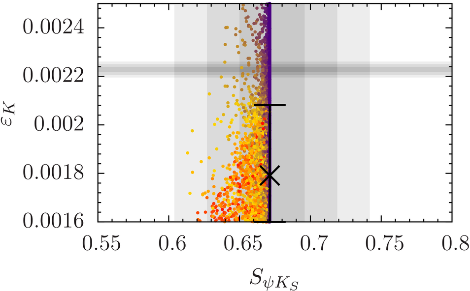
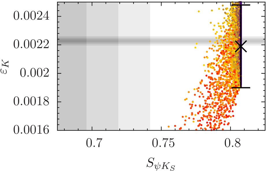
Refer to caption
(a) Exclusive ๐‘ฝ๐’–โ€‹๐’ƒsubscript๐‘ฝ๐’–๐’ƒV_{ub}
Refer to caption
(b) Inclusive ๐‘ฝ๐’–โ€‹๐’ƒsubscript๐‘ฝ๐’–๐’ƒV_{ub}
Figure 3: The correlation of ๐›†๐Šsubscript๐›†๐Š\varepsilon_{K} and ๐’๐›™โ€‹๐Š๐’subscript๐’๐›™subscript๐Š๐’S_{\psi K_{S}}. The shaded grey regions are the experimental ๐Ÿโ€‹๐›”1๐›”1\sigma-๐Ÿ‘โ€‹๐›”3๐›”3\sigma error ranges, while the cross is the central SM values reported in tab.ย 4. The colour of the points represent the percentage of the box-diagram contributions (purple) and of the flavour gauge boson ones (red) in ๐›†๐Šsubscript๐›†๐Š\varepsilon_{K}. In the NP points the theoretical error on ๐›†๐Šsubscript๐›†๐Š\varepsilon_{K} is included.

In fig.ย 3a, we show the correlation between ๐œบ๐‘ฒsubscript๐œบ๐‘ฒ\varepsilon_{K} and ๐‘บ๐โ€‹๐‘ฒ๐‘บsubscript๐‘บ๐subscript๐‘ฒ๐‘บS_{\psi K_{S}}. The plot confirms that the exclusive value of |๐‘ฝ๐’–โ€‹๐’ƒ|subscript๐‘ฝ๐’–๐’ƒ|V_{ub}| is favoured in this model. Indeed the NP contributions are able to solve the ๐œบ๐‘ฒsubscript๐œบ๐‘ฒ\varepsilon_{K}โ€“๐‘บ๐โ€‹๐‘ฒ๐‘บsubscript๐‘บ๐subscript๐‘ฒ๐‘บS_{\psi K_{S}} anomaly in a reasonably large region of the parameters space. This happens when the ๐œบ๐‘ฒsubscript๐œบ๐‘ฒ\varepsilon_{K} prediction approaches the data due to box-diagram contributions (purple points), while ๐‘บ๐โ€‹๐‘ฒ๐‘บsubscript๐‘บ๐subscript๐‘ฒ๐‘บS_{\psi K_{S}} is mostly unaffected. This is in particular possible when the flavour gauge bosons contributions are negligible. When the flavour gauge boson contributions are significant (red points) ๐‘บ๐โ€‹๐‘ฒ๐‘บsubscript๐‘บ๐subscript๐‘ฒ๐‘บS_{\psi K_{S}} is uniquely suppressed relatively to the SM value. However, as seen in the figure a combination of large box contributions as well as flavour gauge boson contributions (yellow points) allows bringing ๐œบ๐‘ฒsubscript๐œบ๐‘ฒ\varepsilon_{K} in agreement with the data while keeping ๐‘บ๐โ€‹๐‘ฒ๐‘บsubscript๐‘บ๐subscript๐‘ฒ๐‘บS_{\psi K_{S}} within the ๐Ÿโ€‹๐ˆ2๐ˆ2\sigma experimental error range.

On the other hand, points for which the box contributions are negligible and instead the flavour gauge boson contributions dominate in ๐œบ๐‘ฒsubscript๐œบ๐‘ฒ\varepsilon_{K} (purely red points) cannot explain the observed value of ๐œบ๐‘ฒsubscript๐œบ๐‘ฒ\varepsilon_{K}. However, this kind of contributions are best suited for the case with the inclusive determination of |๐‘ฝ๐’–โ€‹๐’ƒ|subscript๐‘ฝ๐’–๐’ƒ|V_{ub}|, reported in fig.ย 3b. Still, there exist no points, which simultaneously bring ๐œบ๐‘ฒsubscript๐œบ๐‘ฒ\varepsilon_{K} and ๐‘บ๐โ€‹๐‘ฒ๐‘บsubscript๐‘บ๐subscript๐‘ฒ๐‘บS_{\psi K_{S}} in a ๐Ÿ‘โ€‹๐ˆ3๐ˆ3\sigma agreement. The flavour gauge bosons contributions are not large enough to suitably correct ๐‘บ๐โ€‹๐‘ฒ๐‘บsubscript๐‘บ๐subscript๐‘ฒ๐‘บS_{\psi K_{S}}. We conclude that the inclusive determination of |๐‘ฝ๐’–โ€‹๐’ƒ|subscript๐‘ฝ๐’–๐’ƒ|V_{ub}| is disfavoured in this model and we shall not further pursue this case.
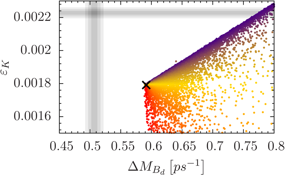
Refer to caption
(a) ๐‘ญ๐‘ฉ๐’…=๐Ÿ๐ŸŽ๐Ÿ“โ€‹๐Œ๐ž๐•subscript๐‘ญsubscript๐‘ฉ๐’…205๐Œ๐ž๐•F_{B_{d}}=205\,{\rm MeV}
Refer to caption
(b) ๐‘ญ๐‘ฉ๐’”=๐Ÿ๐Ÿ“๐ŸŽโ€‹๐Œ๐ž๐•subscript๐‘ญsubscript๐‘ฉ๐’”250๐Œ๐ž๐•F_{B_{s}}=250\,{\rm MeV}
Refer to caption
(c) ๐‘ญ๐‘ฉ๐’…=๐Ÿ๐Ÿ•๐Ÿ“โ€‹๐Œ๐ž๐•subscript๐‘ญsubscript๐‘ฉ๐’…175๐Œ๐ž๐•F_{B_{d}}=175\,{\rm MeV}
Refer to caption
(d) ๐‘ญ๐‘ฉ๐’”=๐Ÿ๐Ÿ๐Ÿ“โ€‹๐Œ๐ž๐•subscript๐‘ญsubscript๐‘ฉ๐’”225๐Œ๐ž๐•F_{B_{s}}=225\,{\rm MeV}
Figure 4: Correlation plot of ๐›†๐Šsubscript๐›†๐Š\varepsilon_{K} with ๐šซโ€‹๐Œ๐๐๐šซsubscript๐Œsubscript๐๐\Delta M_{B_{d}} and ๐šซโ€‹๐Œ๐๐ฌ๐šซsubscript๐Œsubscript๐๐ฌ\Delta M_{B_{s}} on the left and right, respectively. In the upper plots, we use for ๐…๐๐,๐ฌsubscript๐…subscript๐๐๐ฌF_{B_{d,s}} the values reported in tab.ย 3, while for the lower plots we adopt smaller values: ๐…๐๐subscript๐…subscript๐๐F_{B_{d}} is reduced down to ๐Ÿ–๐Ÿ“%percent8585\% of its value, close to the ๐Ÿ‘โ€‹๐›”3๐›”3\sigma error level and ๐…๐๐ฌsubscript๐…subscript๐๐ฌF_{B_{s}} is taken to be the new determination reported in Ref.ย [47]. In the plots above we have not included the ๐Ÿโ€‹๐›”1๐›”1\sigma error in ๐›†๐Šsubscript๐›†๐Š\varepsilon_{K} to best illustrate the interplay of box- (purple) and tree-contributions (red).

In fig.ย 4, we present the correlations between ๐œบ๐‘ฒsubscript๐œบ๐‘ฒ\varepsilon_{K} and ๐šซโ€‹๐‘ด๐‘ฉ๐’…,๐’”๐šซsubscript๐‘ดsubscript๐‘ฉ๐’…๐’”\Delta M_{B_{d,s}}. From LABEL:sub@fig:eK_DeltaMB_a and LABEL:sub@fig:eK_DeltaMB_b, we conclude that the model cannot solve the |๐œบ๐‘ฒ|โˆ’๐‘บ๐โ€‹๐‘ฒ๐‘บsubscript๐œบ๐‘ฒsubscript๐‘บ๐subscript๐‘ฒ๐‘บ|\varepsilon_{K}|-S_{\psi K_{S}} anomaly present in the SM, without worsening the already moderate agreement of this model with the ๐šซโ€‹๐‘ด๐‘ฉ๐’…,๐’”๐šซsubscript๐‘ดsubscript๐‘ฉ๐’…๐’”\Delta M_{B_{d,s}} experimental data. Indeed the values ๐šซโ€‹๐‘ด๐‘ฉ๐’…โ‰ˆ0.75/๐’‘โ€‹๐’”๐šซsubscript๐‘ดsubscript๐‘ฉ๐’…0.75๐’‘๐’”\Delta M_{B_{d}}\approx 0.75/ps and ๐šซโ€‹๐‘ด๐‘ฉ๐’”โ‰ˆ๐Ÿ๐Ÿ•/๐’‘โ€‹๐’”๐šซsubscript๐‘ดsubscript๐‘ฉ๐’”27๐’‘๐’”\Delta M_{B_{s}}\approx 27/ps are so larger that in the case that the central values of the weak decay constants ๐‘ญ๐‘ฉ๐’…,๐’”subscript๐‘ญsubscript๐‘ฉ๐’…๐’”F_{B_{d,s}} do not change in the future, but their and other input parameter uncertainties are further reduced, we will have to conclude that the model fails to describe the ๐šซโ€‹๐‘ญ=๐Ÿ๐šซ๐‘ญ2\Delta F=2 data.

However, we should emphasise that this problem could be avoided if the values for the weak decay constants ๐‘ญ๐‘ฉ๐’…,๐’”subscript๐‘ญsubscript๐‘ฉ๐’…๐’”F_{B_{d,s}} are smaller than the ones used in the plots LABEL:sub@fig:eK_DeltaMB_a and LABEL:sub@fig:eK_DeltaMB_b. Indeed, in LABEL:sub@fig:eK_DeltaMB_c we adopt a ๐Ÿ๐Ÿ“%percent1515\% reduced value for ๐‘ญ๐‘ฉ๐’…subscript๐‘ญsubscript๐‘ฉ๐’…F_{B_{d}}, close to its ๐Ÿ‘โ€‹๐ˆ3๐ˆ3\sigma value, while in LABEL:sub@fig:eK_DeltaMB_d the last determination of ๐‘ญ๐‘ฉ๐’”subscript๐‘ญsubscript๐‘ฉ๐’”F_{B_{s}} reported in Ref.ย [47]. This input, modifies the SM values to be

๐šซโ€‹๐‘ด๐‘ฉ๐’…=0.43โ€‹๐ฉ๐ฌโˆ’๐Ÿand๐šซโ€‹๐‘ด๐‘ฉ๐’”=16.4โ€‹๐ฉ๐ฌโˆ’๐Ÿ,formulae-sequence๐šซsubscript๐‘ดsubscript๐‘ฉ๐’…0.43superscript๐ฉ๐ฌ1and๐šซsubscript๐‘ดsubscript๐‘ฉ๐’”16.4superscript๐ฉ๐ฌ1\Delta M_{B_{d}}=0.43\,{\rm ps}^{-1}\,\qquad\text{and}\qquad\Delta M_{B_{s}}=16.4\,{\rm ps}^{-1}\,, (6.8)

such that now the enhancements of these observables by NP is welcomed by the data. From plots LABEL:sub@fig:eK_DeltaMB_c and LABEL:sub@fig:eK_DeltaMB_d we deduce that the NP contributions and the requirement of agreement of |๐œบ๐‘ฒ|subscript๐œบ๐‘ฒ|\varepsilon_{K}| with data within MGF automatically enhance ๐šซโ€‹๐‘ด๐‘ฉ๐’…,๐’”๐šซsubscript๐‘ดsubscript๐‘ฉ๐’…๐’”\Delta M_{B_{d,s}}. Even if also in this case ๐šซโ€‹๐‘ด๐‘ฉ๐’…,๐’”๐šซsubscript๐‘ดsubscript๐‘ฉ๐’…๐’”\Delta M_{B_{d,s}} are found above the data, the model is performing much better than in the previous case. This exercise shows that on one hand it is crucial to get a better control over hadronic parameters in order to obtain a clearer picture of NP contributions and on the other hand that other more precise observables should be analysed until the uncertainties on ๐šซโ€‹๐‘ด๐‘ฉ๐’…,๐’”๐šซsubscript๐‘ดsubscript๐‘ฉ๐’…๐’”\Delta M_{B_{d,s}} are lowered.

Refer to caption
Refer to caption
Figure 5: Correlation plot for ๐‘๐šซโ€‹๐Œ๐subscript๐‘๐šซsubscript๐Œ๐R_{\Delta M_{B}} and ๐‘๐โ€‹๐‘/๐šซโ€‹๐Œsubscript๐‘๐๐‘๐šซ๐ŒR_{BR/\Delta M}. The grey regions refer to the experimental ๐Ÿโ€‹๐›”1๐›”1\sigma-๐Ÿ‘โ€‹๐›”3๐›”3\sigma and ๐Ÿโ€‹๐›”2๐›”2\sigma-๐Ÿ‘โ€‹๐›”3๐›”3\sigma error ranges for ๐‘๐šซโ€‹๐Œ๐subscript๐‘๐šซsubscript๐Œ๐R_{\Delta M_{B}} and ๐‘๐โ€‹๐‘/๐šซโ€‹๐Œsubscript๐‘๐๐‘๐šซ๐ŒR_{BR/\Delta M}, respectively. The big black point refers to the SM values reported in tab.ย 4. On the left, red (blue) points refer to agreement (disagreement) of the points prediction of ๐›†๐Šsubscript๐›†๐Š\varepsilon_{K} and the data at ๐Ÿ‘โ€‹๐›”3๐›”3\sigma level. On the right the colours represent contribution of boxes and trees in ๐›†๐Šsubscript๐›†๐Š\varepsilon_{K}.

In fig.ย 5, we show the correlation between the ratio of the mass differences, ๐‘น๐šซโ€‹๐‘ด๐‘ฉsubscript๐‘น๐šซsubscript๐‘ด๐‘ฉR_{\Delta M_{B}}, and the ratio among the branching ratio of the ๐‘ฉ+โ†’๐‰+โ€‹๐‚bold-โ†’superscript๐‘ฉsuperscript๐‰๐‚B^{+}\to\tau^{+}\nu decay and the ๐šซโ€‹๐‘ด๐‘ฉ๐’…๐šซsubscript๐‘ดsubscript๐‘ฉ๐’…\Delta M_{B_{d}}, ๐‘น๐‘ฉโ€‹๐‘น/๐šซโ€‹๐‘ดsubscript๐‘น๐‘ฉ๐‘น๐šซ๐‘ดR_{BR/\Delta M}. Both observables have negligible theoretical uncertainties and are therefore very useful to provide strong constraints on the parameter space. On the left, the red points correspond to an ๐œบ๐‘ฒsubscript๐œบ๐‘ฒ\varepsilon_{K} prediction in agreement with the data at ๐Ÿ‘โ€‹๐ˆ3๐ˆ3\sigma, while the blue ones do not satisfy the ๐œบ๐‘ฒsubscript๐œบ๐‘ฒ\varepsilon_{K} constraint. This plot largely constrains the parameter space of the model; for only very few points ๐œบ๐‘ฒsubscript๐œบ๐‘ฒ\varepsilon_{K}, ๐‘น๐šซโ€‹๐‘ด๐‘ฉsubscript๐‘น๐šซsubscript๐‘ด๐‘ฉR_{\Delta M_{B}} and ๐‘น๐‘ฉโ€‹๐‘น/๐šซโ€‹๐‘ดsubscript๐‘น๐‘ฉ๐‘น๐šซ๐‘ดR_{BR/\Delta M} agree at ๐Ÿ‘โ€‹๐ˆ3๐ˆ3\sigma-level with the data simultaneously.

Furthermore, all red points correspond to values for ๐‘น๐‘ฉโ€‹๐‘น/๐šซโ€‹๐‘ดsubscript๐‘น๐‘ฉ๐‘น๐šซ๐‘ดR_{BR/\Delta M} smaller than the SM prediction and therefore the model can only worsen the SM tension. In the case that the experimental sensitivity to the ๐‘ฉโ€‹๐‘นโ€‹(๐‘ฉ+โ†’๐‰+โ€‹๐‚)๐‘ฉ๐‘นbold-โ†’superscript๐‘ฉsuperscript๐‰๐‚BR(B^{+}\to\tau^{+}\nu) improves, it will be possible to further constrain and possible exclude the present MGF model.
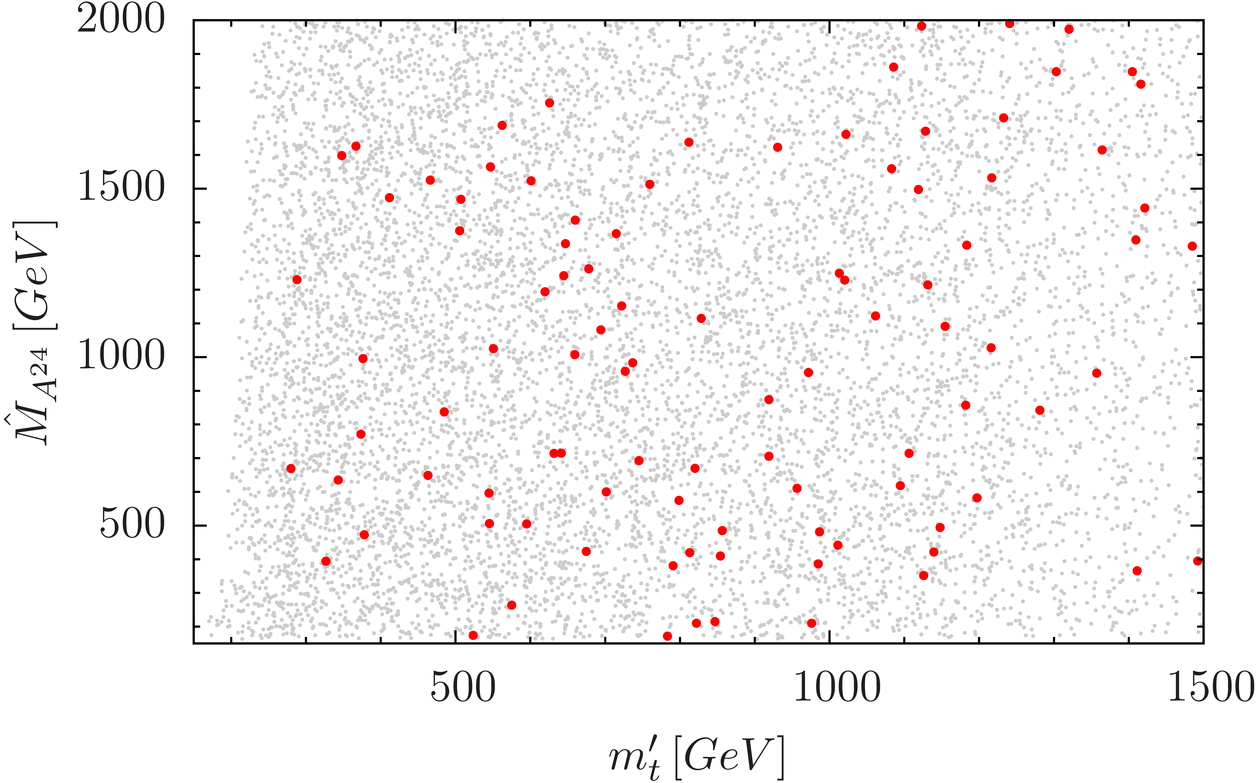
Refer to caption
Figure 6: ๐’Ž๐’•โ€ฒโˆ’๐‘ด^๐‘จ๐Ÿ๐Ÿ’subscript๐’Žsuperscript๐’•bold-โ€ฒsubscriptbold-^๐‘ดsuperscript๐‘จ24m_{t^{\prime}}-\hat{M}_{A^{24}} parameter space. For all red points in the plot ๐‘๐šซโ€‹๐Œ๐subscript๐‘๐šซsubscript๐Œ๐R_{\Delta M_{B}}, ๐‘๐โ€‹๐‘/๐šซโ€‹๐Œsubscript๐‘๐๐‘๐šซ๐ŒR_{BR/\Delta M} and ๐›†๐Šsubscript๐›†๐Š\varepsilon_{K} agree with the data at ๐Ÿ‘โ€‹๐›”3๐›”3\sigma-level.

Having reduced the parameter space, we concentrate now on a few other predictions of the model. In fig.ย 6, we show the ๐’Ž๐’•โ€ฒโˆ’๐‘ด^๐‘จ๐Ÿ๐Ÿ’subscript๐’Žsuperscript๐’•bold-โ€ฒsubscriptbold-^๐‘ดsuperscript๐‘จ24m_{t^{\prime}}-\hat{M}_{A^{24}} parameter space, where ๐’Ž๐’•โ€ฒsubscript๐’Žsuperscript๐’•bold-โ€ฒm_{t^{\prime}} is the mass of the exotic partner of the top-quark and ๐‘ด^๐‘จ๐Ÿ๐Ÿ’subscriptbold-^๐‘ดsuperscript๐‘จ24\hat{M}_{A^{24}} the mass of the lightest neutral gauge boson; the corresponding particles have the best chances to be detected at the LHC. The red and blue points are those identified in fig.ย 5 to agree and disagree in ๐‘น๐šซโ€‹๐‘ด๐‘ฉsubscript๐‘น๐šซsubscript๐‘ด๐‘ฉR_{\Delta M_{B}}, ๐‘น๐‘ฉโ€‹๐‘น/๐šซโ€‹๐‘ดsubscript๐‘น๐‘ฉ๐‘น๐šซ๐‘ดR_{BR/\Delta M} and ๐œบ๐‘ฒsubscript๐œบ๐‘ฒ\varepsilon_{K} with the data at the ๐Ÿโ€‹๐ˆ1๐ˆ1\sigma-๐Ÿ‘โ€‹๐ˆ3๐ˆ3\sigma level, respectively.

Interestingly, the phenomenological results presented above hold not only for light but also for heavy ๐’•โ€ฒsuperscript๐’•bold-โ€ฒt^{\prime}โ€™s. Also the mass of the lightest flavour gauge boson is not bounded.
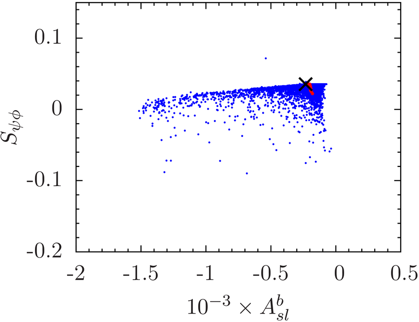
Refer to caption
(a)
Refer to caption
(b)
Figure 7: Correlation plot of ๐’๐›™โ€‹ฯ•subscript๐’๐›™bold-ฯ•S_{\psi\phi} and ๐€๐ฌโ€‹๐ฅ๐›subscriptsuperscript๐€๐›๐ฌ๐ฅA^{b}_{sl} on the left and ๐โ€‹๐‘โ€‹(๐ยฏโ†’๐—๐ฌโ€‹๐›„)๐๐‘bold-โ†’bold-ยฏ๐subscript๐—๐ฌ๐›„BR(\bar{B}\to X_{s}\gamma) and ๐ฆ๐ญโ€ฒsuperscriptsubscript๐ฆ๐ญbold-โ€ฒm_{t}^{\prime} on the right. Grey regions refer to the experimental error ranges. The big black point refers to the SM values reported in tab.ย 4. In red the points for which ๐‘๐šซโ€‹๐Œ๐subscript๐‘๐šซsubscript๐Œ๐R_{\Delta M_{B}}, ๐‘๐โ€‹๐‘/๐šซโ€‹๐Œsubscript๐‘๐๐‘๐šซ๐ŒR_{BR/\Delta M} and ๐›†๐Šsubscript๐›†๐Š\varepsilon_{K} agree with the data at ๐Ÿ‘โ€‹๐›”3๐›”3\sigma level, in blue all others for which there is no agreement.

Furthermore, in fig.ย 7 we show two correlation plots which represent also clear predictions for this model. Plot LABEL:sub@fig:SpsiphiAbsl is the correlation for ๐‘บ๐โ€‹ฯ•subscript๐‘บ๐bold-italic-ฯ•S_{\psi\phi} and ๐‘จ๐’”โ€‹๐’๐’ƒsubscriptsuperscript๐‘จ๐’ƒ๐’”๐’A^{b}_{sl} showing that only tiny deviations from the SM values are allowed: this turns out to be an interesting result for ๐‘บ๐โ€‹ฯ•subscript๐‘บ๐bold-italic-ฯ•S_{\psi\phi}, which is indeed close to the recent determination of LHCb. On the other hand, ๐‘จ๐’”โ€‹๐’๐’ƒsubscriptsuperscript๐‘จ๐’ƒ๐’”๐’A^{b}_{sl} has only been measured by D0, but hopefully LHCb will also have something to say in the near future. Once the experimental uncertainties are lowered, such clear predictions will be essential to provide the final answer on how well this model performs.

In plot LABEL:sub@fig:BSgammamtp, we show the correlation of ๐‘ฉโ€‹๐‘นโ€‹(๐‘ฉยฏโ†’๐‘ฟ๐’”โ€‹๐œธ)๐‘ฉ๐‘นbold-โ†’bold-ยฏ๐‘ฉsubscript๐‘ฟ๐’”๐œธBR(\bar{B}\to X_{s}\gamma) and ๐’Ž๐’•โ€ฒsuperscriptsubscript๐’Ž๐’•bold-โ€ฒm_{t}^{\prime}. We confirm the finding of Grinstein et al. that in this model the NP contributions to ๐‘ฉโ€‹๐‘นโ€‹(๐‘ฉโ†’๐‘ฟ๐’”โ€‹๐œธ)๐‘ฉ๐‘นbold-โ†’๐‘ฉsubscript๐‘ฟ๐’”๐œธBR(B\to X_{s}\gamma) always enhance it towards the central experiment value. However, interestingly only very small enhancements of this branching ratio are allowed when also the bounds from ๐šซโ€‹๐‘ญ=๐Ÿ๐šซ๐‘ญ2\Delta F=2 observables are taken into account.

7 Comparison with other Models

A complete comparison of the patterns of flavour violation in MGF with corresponding patterns found in numerous models [51] would require the study of ๐šซโ€‹๐‘ญ=๐Ÿ๐šซ๐‘ญ1\Delta F=1 processes, however already ๐šซโ€‹๐‘ญ=๐Ÿ๐šซ๐‘ญ2\Delta F=2 observables allow a clear distinction between the MGF and the simplest extensions of the SM. Here we just quote a few examples:

  • -

    In the original MFV framework restricted to LL operators, the so-called constrained MFV [52], the |๐œบ๐‘ฒ|โˆ’๐‘บ๐โ€‹๐‘ฒ๐‘บsubscript๐œบ๐‘ฒsubscript๐‘บ๐subscript๐‘ฒ๐‘บ|\varepsilon_{K}|-S_{\psi K_{S}} anomaly can only be solved by enhancing |๐œบ๐‘ฒ|subscript๐œบ๐‘ฒ|\varepsilon_{K}| since in this framework ๐‘บ๐โ€‹๐‘ฒ๐‘บsubscript๐‘บ๐subscript๐‘ฒ๐‘บS_{\psi K_{S}} remains SM-like. In this framework then only the exclusive value of |๐‘ฝ๐’–โ€‹๐’ƒ|subscript๐‘ฝ๐’–๐’ƒ|V_{ub}| is viable. An example of such a framework is the model with a single universal extra dimension (UED) for which a very detailed analysis of ๐šซโ€‹๐‘ญ=๐Ÿ๐šซ๐‘ญ2\Delta F=2 observables has been performed in [53]. In fact this is a general property of CMFV models as demonstrated in [54]. Thus after |๐œบ๐‘ฒ|subscript๐œบ๐‘ฒ|\varepsilon_{K}| has been taken into account and contributions from tree-level heavy gauge boson exchanges have been eliminated MGF resembles CMFV if only ๐šซโ€‹๐‘ญ=๐Ÿ๐šซ๐‘ญ2\Delta F=2 processes are considered. However ๐šซโ€‹๐‘ญ=๐Ÿ๐šซ๐‘ญ1\Delta F=1 processes can provide a distinction. In fact whereas in MGF the NP contributions uniquely enhance ๐‘ฉโ€‹๐‘นโ€‹(๐‘ฉยฏโ†’๐‘ฟ๐’”โ€‹๐œธ)๐‘ฉ๐‘นbold-โ†’bold-ยฏ๐‘ฉsubscript๐‘ฟ๐’”๐œธBR(\overline{B}\to X_{s}\gamma), in UED they uniquely suppress this branching ratio [55]. Concerning the |๐œบ๐‘ฒ|subscript๐œบ๐‘ฒ|\varepsilon_{K}|โ€“๐šซโ€‹๐‘ด๐‘ฉ๐’…,๐’”๐šซsubscript๐‘ดsubscript๐‘ฉ๐’…๐’”\Delta M_{B_{d,s}} tension MGF and CMFV are again similar.

  • -

    The 2HDM framework with MFV and flavour blind phases, the so-called ๐Ÿโ€‹๐‡โ€‹๐ƒโ€‹๐Œ๐Œ๐…๐•ยฏ2๐‡๐ƒsubscript๐Œbold-ยฏ๐Œ๐…๐•{\rm 2HDM_{\overline{MFV}}} [56], can on the other hand be easily distinguished from MGF. In this model NP contributions to ๐œบ๐‘ฒsubscript๐œบ๐‘ฒ\varepsilon_{K} are tiny and the inclusive value of |๐‘ฝ๐’–โ€‹๐’ƒ|subscript๐‘ฝ๐’–๐’ƒ|V_{ub}| is required in order to obtain the correct value of |๐œบ๐‘ฒ|subscript๐œบ๐‘ฒ|\varepsilon_{K}|. The interplay of the CKM phase with the flavour blind phases in Yukawa couplings and Higgs potential suppress ๐‘บ๐โ€‹๐‘ฒ๐‘บsubscript๐‘บ๐subscript๐‘ฒ๐‘บS_{\psi K_{S}} simultaneously enhancing the asymmetry ๐‘บ๐โ€‹ฯ•subscript๐‘บ๐bold-italic-ฯ•S_{\psi\phi}. As in the case of MGF this asymmetry is SM-like or has a reversed sign. It is ๐‘บ๐โ€‹ฯ•subscript๐‘บ๐bold-italic-ฯ•S_{\psi\phi} together with the value of |๐‘ฝ๐’–โ€‹๐’ƒ|subscript๐‘ฝ๐’–๐’ƒ|V_{ub}| which will distinguish MGF from ๐Ÿโ€‹๐‡โ€‹๐ƒโ€‹๐Œ๐Œ๐…๐•ยฏ2๐‡๐ƒsubscript๐Œbold-ยฏ๐Œ๐…๐•{\rm 2HDM_{\overline{MFV}}}.

  • -

    Finally, let us mention the left-right asymmetric model (LRAM) for which a very detailed FCNC analysis has been recently presented in [57]. As this model has many free parameters both values of |๐‘ฝ๐’–โ€‹๐’ƒ|subscript๐‘ฝ๐’–๐’ƒ|V_{ub}|, inclusive and exclusive, are valid. The model contains many new phases and the |๐œบ๐‘ฒ|โˆ’๐‘บ๐โ€‹๐‘ฒ๐‘บsubscript๐œบ๐‘ฒsubscript๐‘บ๐subscript๐‘ฒ๐‘บ|\varepsilon_{K}|-S_{\psi K_{S}} anomaly can be solved in many ways. Moreover, the model struggles with the ๐œบ๐‘ฒsubscript๐œบ๐‘ฒ\varepsilon_{K} constraint due to huge neutral Higgs tree-level contributions. However, as demonstrated in Section 7 of that paper a simple structure of the right-handed mixing matrix gives a transparent solution to the |๐œบ๐‘ฒ|โˆ’๐‘บ๐โ€‹๐‘ฒ๐‘บsubscript๐œบ๐‘ฒsubscript๐‘บ๐subscript๐‘ฒ๐‘บ|\varepsilon_{K}|-S_{\psi K_{S}} anomaly by enhancing |๐œบ๐‘ฒ|subscript๐œบ๐‘ฒ|\varepsilon_{K}|, keeping ๐‘บ๐โ€‹๐‘ฒ๐‘บsubscript๐‘บ๐subscript๐‘ฒ๐‘บS_{\psi K_{S}} at the SM value and in contrast to MGF automatically suppressing ๐šซโ€‹๐‘ด๐‘ฉ๐’…,๐’”๐šซsubscript๐‘ดsubscript๐‘ฉ๐’…๐’”\Delta M_{B_{d,s}} and significantly enhancing ๐‘บ๐โ€‹ฯ•subscript๐‘บ๐bold-italic-ฯ•S_{\psi\phi}. While MGF falls back in this comparison, one should emphasise than on the MGF has very few parameters and provides the explanation of quark masses and mixings, while this is not the case in the LRAM.

8 Conclusion

We have presented an extensive analysis of ๐šซโ€‹๐‘ญ=๐Ÿ๐šซ๐‘ญ2\Delta F=2 observables and ๐‘ฉโ†’๐‘ฟ๐’”โ€‹๐œธbold-โ†’๐‘ฉsubscript๐‘ฟ๐’”๐œธB\to X_{s}\gamma for a specific MGF model presented in Ref.ย [12], which is of special interest due to the small number of new parameters. In particular we performed a detailed study of the effects of tree-level contributions due to the presence of heavy flavour gauge bosons.

Our main findings are as follows. The model predicts a clear pattern of deviations from the SM:

  • -

    Enhancements of |๐œบ๐‘ฒ|subscript๐œบ๐‘ฒ|\varepsilon_{K}| and ๐šซโ€‹๐‘ด๐‘ฉ๐’…,๐’”๐šซsubscript๐‘ดsubscript๐‘ฉ๐’…๐’”\Delta M_{B_{d,s}} in a correlated manner by new box-diagram contributions and suppression of |๐œบ๐‘ฒ|subscript๐œบ๐‘ฒ|\varepsilon_{K}| by tree-level heavy gauge boson contributions with only small impact on ๐šซโ€‹๐‘ด๐‘ฉ๐’…,๐’”๐šซsubscript๐‘ดsubscript๐‘ฉ๐’…๐’”\Delta M_{B_{d,s}}.

  • -

    Mixing induced CP-asymmetries ๐‘บ๐โ€‹๐‘ฒ๐‘บsubscript๐‘บ๐subscript๐‘ฒ๐‘บS_{\psi K_{S}} and ๐‘บ๐โ€‹ฯ•subscript๐‘บ๐bold-italic-ฯ•S_{\psi\phi} are unaffected by box-diagram contributions, but receive sizeable destructive contributions from tree-level heavy gauge boson exchanges such that the sign of ๐‘บ๐โ€‹ฯ•subscript๐‘บ๐bold-italic-ฯ•S_{\psi\phi} can be reversed. However, these effects are basically eliminated once the ๐œบ๐‘ฒsubscript๐œบ๐‘ฒ\varepsilon_{K} constraint is taken into account.

  • -

    The ๐œบ๐‘ฒโˆ’๐‘บ๐โ€‹๐‘ฒ๐‘บsubscript๐œบ๐‘ฒsubscript๐‘บ๐subscript๐‘ฒ๐‘บ\varepsilon_{K}-S_{\psi K_{S}} anomaly present in the SM is removed through the enhancement of |๐œบ๐‘ฒ|subscript๐œบ๐‘ฒ|\varepsilon_{K}|, leaving ๐‘บ๐โ€‹๐‘ฒ๐‘บsubscript๐‘บ๐subscript๐‘ฒ๐‘บS_{\psi K_{S}} practically unmodified. This is achieved with the help of box-diagram contributions in the regions of the parameter space for which they are dominant over heavy flavour gauge boson contributions, which interfere destructively with the SM amplitudes.

  • -

    This structure automatically implies that in this model the exclusive determination of |๐‘ฝ๐’–โ€‹๐’ƒ|subscript๐‘ฝ๐’–๐’ƒ|V_{ub}| is favoured.

  • -

    ๐’ƒ๐’ƒb semileptonic CP-asymmetry ๐‘จ๐’”โ€‹๐’๐’ƒsubscriptsuperscript๐‘จ๐’ƒ๐’”๐’A^{b}_{sl}, that a priori could receive large contributions from the tree-level flavour gauge boson diagrams, remains close to the SM values once requiring |๐œบ๐‘ฒ|subscript๐œบ๐‘ฒ|\varepsilon_{K}| to be in agreement with the data.

  • -

    Most importantly, the ๐œบ๐‘ฒsubscript๐œบ๐‘ฒ\varepsilon_{K} constraint implies the central values of ๐šซโ€‹๐‘ด๐‘ฉ๐’…,๐’”๐šซsubscript๐‘ดsubscript๐‘ฉ๐’…๐’”\Delta M_{B_{d,s}} to be roughly ๐Ÿ“๐ŸŽ%percent5050\% higher than the very precise data. This disagreement cannot be cured fully by hadronic uncertainties although significant reduction in the values of ๐‘ญ๐‘ฉ๐’…,๐’”subscript๐‘ญsubscript๐‘ฉ๐’…๐’”F_{B_{d,s}} could soften this problem.

  • -

    We have pointed out that the ratio of the mass differences, ๐šซโ€‹๐‘ด๐‘ฉ๐’…/๐šซโ€‹๐‘ด๐‘ฉ๐’”๐šซsubscript๐‘ดsubscript๐‘ฉ๐’…๐šซsubscript๐‘ดsubscript๐‘ฉ๐’”\Delta M_{B_{d}}/\Delta M_{B_{s}} and the ratio of the ๐‘ฉ+โ†’๐‰+โ€‹๐‚bold-โ†’superscript๐‘ฉsuperscript๐‰๐‚B^{+}\to\tau^{+}\nu branching ratio and ๐šซโ€‹๐‘ด๐‘ฉ๐’…๐šซsubscript๐‘ดsubscript๐‘ฉ๐’…\Delta M_{B_{d}}, together with ๐œบ๐‘ฒsubscript๐œบ๐‘ฒ\varepsilon_{K}, provide strong constraints on the parameter space of the model. Furthermore, the correlation among these two observables encodes a serious tension on the flavour data that can only be deteriorated in the model.

  • -

    In agreement with Ref.ย [12], we find that ๐‘ฉโ€‹๐‘นโ€‹(๐‘ฉโ†’๐‘ฟ๐’”โ€‹๐œธ)๐‘ฉ๐‘นbold-โ†’๐‘ฉsubscript๐‘ฟ๐’”๐œธBR(B\to X_{s}\gamma) is naturally enhanced in this model, bringing the theory closer to the data, still only small corrections are allowed by the ๐šซโ€‹๐‘ญ=๐Ÿ๐šซ๐‘ญ2\Delta F=2 bounds.

  • -

    We have demonstrated how this model can be distinguished by means of the flavour data from other extensions of the SM.

In summary, the great virtue of this model is its predictivity, such that within the coming years it will be evident whether it can be considered as a valid description of low-energy data. Possibly the most transparent viability tests of the model are the future values of ๐‘ญ๐‘ฉ๐’…,๐’”subscript๐‘ญsubscript๐‘ฉ๐’…๐’”F_{B_{d,s}} and |๐‘ฝ๐’–โ€‹๐’ƒ|subscript๐‘ฝ๐’–๐’ƒ|V_{ub}|. For the model to accommodate the data, ๐‘ญ๐‘ฉ๐’…,๐’”subscript๐‘ญsubscript๐‘ฉ๐’…๐’”F_{B_{d,s}} have to be reduced by ๐Ÿ๐Ÿ“%percent1515\% and |๐‘ฝ๐’–โ€‹๐’ƒ|subscript๐‘ฝ๐’–๐’ƒ|V_{ub}| has to be close to 3.4ร—๐Ÿ๐ŸŽโˆ’๐Ÿ‘3.4superscript1033.4\times 10^{-3}. Violation of any of these requirements will put this extension of the SM in trouble. We emphasise that the triple correlation between ๐šซโ€‹๐‘ด๐‘ฉ๐’…,๐’”๐šซsubscript๐‘ดsubscript๐‘ฉ๐’…๐’”\Delta M_{B_{d,s}}, ๐œบ๐‘ฒsubscript๐œบ๐‘ฒ\varepsilon_{K} and ๐‘บ๐โ€‹๐‘ฒ๐‘บsubscript๐‘บ๐subscript๐‘ฒ๐‘บS_{\psi K_{S}} was instrumental in reaching this conclusion. The same result is derived by the complementary study on the ๐‘น๐‘ฉโ€‹๐‘น/๐šซโ€‹๐‘ดโˆ’๐‘น๐šซโ€‹๐‘ด๐‘ฉsubscript๐‘น๐‘ฉ๐‘น๐šซ๐‘ดsubscript๐‘น๐šซsubscript๐‘ด๐‘ฉR_{BR/\Delta M}-R_{\Delta M_{B}} correlation. Our work shows that the study of correlations among flavour observables and the accuracy of non-perturbative parameters like ๐‘ฉ^๐‘ฒsubscriptbold-^๐‘ฉ๐‘ฒ\hat{B}_{K} and ๐‘ญ๐‘ฉ๐’…,๐’”subscript๐‘ญsubscript๐‘ฉ๐’…๐’”F_{B_{d,s}} are crucial for the indirect searches for physics beyond the Standard Model.

Acknowledgements

We would like to thank Benjamรญn Grinstein for useful details on the Ref.ย [12], Ulrich Nierste and Paride Paradisi for very interesting discussions. This research was done in the context of the ERC Advanced Grant project โ€FLAVOURโ€(267104). The work of MVC has been partially supported by the Graduiertenkolleg GRK 1054 of DFG.

Appendix A Feynman Rules for MGF

A.1 Couplings of SM Gauge and Goldstone bosons

๐œธ๐œธ\gamma coupling

The photon coupling remains unchanged; proportional to the quark charges ๐‘ธ๐’–subscript๐‘ธ๐’–Q_{u} and ๐‘ธ๐’…subscript๐‘ธ๐’…Q_{d}.

๐‘ฎ๐‘ฎG coupling

The gluon coupling remains unchanged; proportional to the colour generators ๐€๐‘บโ€‹๐‘ผโ€‹(๐Ÿ‘)๐’‚superscriptsubscript๐€๐‘บ๐‘ผ3๐’‚\lambda_{SU(3)}^{a}.

๐‘พยฑsuperscript๐‘พplus-or-minusW^{\pm} coupling

[Uncaptioned image]

with the actual values for ๐’‡ยฏbold-ยฏ๐’‡\bar{f}, ๐’‡๐’‡f and ๐‘ช๐‘ณsubscript๐‘ช๐‘ณC_{L}:

๐‘พ+โ€‹๐’–ยฏ๐’Šโ€‹๐’…๐’‹superscript๐‘พsubscriptbold-ยฏ๐’–๐’Šsubscript๐’…๐’‹W^{+}\bar{u}_{i}d_{j} : ๐‘ช๐‘ณ=๐’„๐’–โ€‹๐‘ณโ€‹๐’Šโ€‹๐‘ฝ๐’Šโ€‹๐’‹โ€‹๐’„๐’…โ€‹๐‘ณโ€‹๐’‹subscript๐‘ช๐‘ณsubscript๐’„๐’–๐‘ณ๐’Šsubscript๐‘ฝ๐’Š๐’‹subscript๐’„๐’…๐‘ณ๐’‹C_{L}=c_{uLi}V_{ij}c_{dLj}
๐‘พ+โ€‹๐’–ยฏ๐’Šโ€ฒโ€‹๐’…๐’‹โ€ฒsuperscript๐‘พsubscriptsuperscriptbold-ยฏ๐’–bold-โ€ฒ๐’Šsubscriptsuperscript๐’…bold-โ€ฒ๐’‹W^{+}\bar{u}^{\prime}_{i}d^{\prime}_{j} : ๐‘ช๐‘ณ=๐’”๐’–โ€‹๐‘ณโ€‹๐’Šโ€‹๐‘ฝ๐’Šโ€‹๐’‹โ€‹๐’”๐’…โ€‹๐‘ณโ€‹๐’‹subscript๐‘ช๐‘ณsubscript๐’”๐’–๐‘ณ๐’Šsubscript๐‘ฝ๐’Š๐’‹subscript๐’”๐’…๐‘ณ๐’‹C_{L}=s_{uLi}V_{ij}s_{dLj}
๐‘พ+โ€‹๐’–ยฏ๐’Šโ€‹๐’…๐’‹โ€ฒsuperscript๐‘พsubscriptbold-ยฏ๐’–๐’Šsubscriptsuperscript๐’…bold-โ€ฒ๐’‹W^{+}\bar{u}_{i}d^{\prime}_{j} : ๐‘ช๐‘ณ=๐’„๐’–โ€‹๐‘ณโ€‹๐’Šโ€‹๐‘ฝ๐’Šโ€‹๐’‹โ€‹๐’”๐’…โ€‹๐‘ณโ€‹๐’‹subscript๐‘ช๐‘ณsubscript๐’„๐’–๐‘ณ๐’Šsubscript๐‘ฝ๐’Š๐’‹subscript๐’”๐’…๐‘ณ๐’‹C_{L}=c_{uLi}V_{ij}s_{dLj}
๐‘พ+โ€‹๐’–ยฏ๐’Šโ€ฒโ€‹๐’…๐’‹superscript๐‘พsubscriptsuperscriptbold-ยฏ๐’–bold-โ€ฒ๐’Šsubscript๐’…๐’‹W^{+}\bar{u}^{\prime}_{i}d_{j} : ๐‘ช๐‘ณ=๐’”๐’–โ€‹๐‘ณโ€‹๐’Šโ€‹๐‘ฝ๐’Šโ€‹๐’‹โ€‹๐’„๐’…โ€‹๐‘ณโ€‹๐’‹subscript๐‘ช๐‘ณsubscript๐’”๐’–๐‘ณ๐’Šsubscript๐‘ฝ๐’Š๐’‹subscript๐’„๐’…๐‘ณ๐’‹C_{L}=s_{uLi}V_{ij}c_{dLj}
๐‘พโˆ’โ€‹๐’…ยฏ๐’‹โ€‹๐’–๐’Šsuperscript๐‘พsubscriptbold-ยฏ๐’…๐’‹subscript๐’–๐’ŠW^{-}\bar{d}_{j}u_{i} : ๐‘ช๐‘ณ=๐’„๐’–โ€‹๐‘ณโ€‹๐’Šโ€‹๐‘ฝ๐’Šโ€‹๐’‹โˆ—โ€‹๐’„๐’…โ€‹๐‘ณโ€‹๐’‹subscript๐‘ช๐‘ณsubscript๐’„๐’–๐‘ณ๐’Šsuperscriptsubscript๐‘ฝ๐’Š๐’‹subscript๐’„๐’…๐‘ณ๐’‹C_{L}=c_{uLi}V_{ij}^{*}c_{dLj}
๐‘พโˆ’โ€‹๐’…ยฏ๐’‹โ€ฒโ€‹๐’–๐’Šโ€ฒsuperscript๐‘พsubscriptsuperscriptbold-ยฏ๐’…bold-โ€ฒ๐’‹subscriptsuperscript๐’–bold-โ€ฒ๐’ŠW^{-}\bar{d}^{\prime}_{j}u^{\prime}_{i} : ๐‘ช๐‘ณ=๐’”๐’–โ€‹๐‘ณโ€‹๐’Šโ€‹๐‘ฝ๐’Šโ€‹๐’‹โˆ—โ€‹๐’”๐’…โ€‹๐‘ณโ€‹๐’‹subscript๐‘ช๐‘ณsubscript๐’”๐’–๐‘ณ๐’Šsuperscriptsubscript๐‘ฝ๐’Š๐’‹subscript๐’”๐’…๐‘ณ๐’‹C_{L}=s_{uLi}V_{ij}^{*}s_{dLj}
๐‘พโˆ’โ€‹๐’…ยฏ๐’‹โ€‹๐’–๐’Šโ€ฒsuperscript๐‘พsubscriptbold-ยฏ๐’…๐’‹subscriptsuperscript๐’–bold-โ€ฒ๐’ŠW^{-}\bar{d}_{j}u^{\prime}_{i} : ๐‘ช๐‘ณ=๐’”๐’–โ€‹๐‘ณโ€‹๐’Šโ€‹๐‘ฝ๐’Šโ€‹๐’‹โˆ—โ€‹๐’„๐’…โ€‹๐‘ณโ€‹๐’‹subscript๐‘ช๐‘ณsubscript๐’”๐’–๐‘ณ๐’Šsuperscriptsubscript๐‘ฝ๐’Š๐’‹subscript๐’„๐’…๐‘ณ๐’‹C_{L}=s_{uLi}V_{ij}^{*}c_{dLj}
๐‘พโˆ’โ€‹๐’…ยฏ๐’‹โ€ฒโ€‹๐’–๐’Šsuperscript๐‘พsubscriptsuperscriptbold-ยฏ๐’…bold-โ€ฒ๐’‹subscript๐’–๐’ŠW^{-}\bar{d}^{\prime}_{j}u_{i} : ๐‘ช๐‘ณ=๐’„๐’–โ€‹๐‘ณโ€‹๐’Šโ€‹๐‘ฝ๐’Šโ€‹๐’‹โˆ—โ€‹๐’”๐’…โ€‹๐‘ณโ€‹๐’‹subscript๐‘ช๐‘ณsubscript๐’„๐’–๐‘ณ๐’Šsuperscriptsubscript๐‘ฝ๐’Š๐’‹subscript๐’”๐’…๐‘ณ๐’‹C_{L}=c_{uLi}V_{ij}^{*}s_{dLj}

๐’๐’Z coupling

[Uncaptioned image]

with the actual values for ๐’‡ยฏbold-ยฏ๐’‡\bar{f}, ๐’‡๐’‡f and C:

๐’โ€‹๐’–ยฏ๐’Šโ€‹๐’–๐’Š๐’subscriptbold-ยฏ๐’–๐’Šsubscript๐’–๐’ŠZ\bar{u}_{i}u_{i} : ๐‘ช๐‘น=โˆ’๐’”๐’˜๐Ÿ๐’„๐’˜โ€‹๐‘ธ๐’–subscript๐‘ช๐‘นsuperscriptsubscript๐’”๐’˜2subscript๐’„๐’˜subscript๐‘ธ๐’–C_{R}=-\frac{s_{w}^{2}}{c_{w}}Q_{u}
: ๐‘ช๐‘ณ=๐‘ป๐’–๐Ÿ‘โ€‹๐’„๐’–โ€‹๐‘ณโ€‹๐’Š๐Ÿโˆ’๐’”๐’˜๐Ÿโ€‹๐‘ธ๐’–๐’„๐’˜subscript๐‘ช๐‘ณsuperscriptsubscript๐‘ป๐’–3superscriptsubscript๐’„๐’–๐‘ณ๐’Š2superscriptsubscript๐’”๐’˜2subscript๐‘ธ๐’–subscript๐’„๐’˜C_{L}=\frac{T_{u}^{3}c_{uLi}^{2}-s_{w}^{2}Q_{u}}{c_{w}}
๐’โ€‹๐’–ยฏ๐’Šโ€ฒโ€‹๐’–๐’Šโ€ฒ๐’subscriptsuperscriptbold-ยฏ๐’–bold-โ€ฒ๐’Šsubscriptsuperscript๐’–bold-โ€ฒ๐’ŠZ\bar{u}^{\prime}_{i}u^{\prime}_{i} : ๐‘ช๐‘น=โˆ’๐’”๐’˜๐Ÿ๐’„๐’˜โ€‹๐‘ธ๐’–subscript๐‘ช๐‘นsuperscriptsubscript๐’”๐’˜2subscript๐’„๐’˜subscript๐‘ธ๐’–C_{R}=-\frac{s_{w}^{2}}{c_{w}}Q_{u}
: ๐‘ช๐‘ณ=+๐‘ป๐’–๐Ÿ‘โ€‹๐’”๐’–โ€‹๐‘ณโ€‹๐’Š๐Ÿโˆ’๐’”๐’˜๐Ÿโ€‹๐‘ธ๐’–๐’„๐’˜subscript๐‘ช๐‘ณsuperscriptsubscript๐‘ป๐’–3superscriptsubscript๐’”๐’–๐‘ณ๐’Š2superscriptsubscript๐’”๐’˜2subscript๐‘ธ๐’–subscript๐’„๐’˜C_{L}=+\frac{T_{u}^{3}s_{uLi}^{2}-s_{w}^{2}Q_{u}}{c_{w}}
๐’โ€‹๐’–ยฏ๐’Šโ€‹๐’–๐’Šโ€ฒ๐’subscriptbold-ยฏ๐’–๐’Šsubscriptsuperscript๐’–bold-โ€ฒ๐’ŠZ\bar{u}_{i}u^{\prime}_{i} : ๐‘ช๐‘น=๐ŸŽsubscript๐‘ช๐‘น0C_{R}=0
: ๐‘ช๐‘ณ=+๐‘ป๐’–๐Ÿ‘๐’„๐’˜โ€‹๐’„๐’–โ€‹๐‘ณโ€‹๐’Šโ€‹๐’”๐’–โ€‹๐‘ณโ€‹๐’Šsubscript๐‘ช๐‘ณsuperscriptsubscript๐‘ป๐’–3subscript๐’„๐’˜subscript๐’„๐’–๐‘ณ๐’Šsubscript๐’”๐’–๐‘ณ๐’ŠC_{L}=+\frac{T_{u}^{3}}{c_{w}}c_{uLi}s_{uLi}
๐’โ€‹๐’–ยฏ๐’Šโ€ฒโ€‹๐’–๐’Š๐’subscriptsuperscriptbold-ยฏ๐’–bold-โ€ฒ๐’Šsubscript๐’–๐’ŠZ\bar{u}^{\prime}_{i}u_{i} : ๐‘ช๐‘น=๐ŸŽsubscript๐‘ช๐‘น0C_{R}=0
: ๐‘ช๐‘ณ=+๐‘ป๐’–๐Ÿ‘๐’„๐’˜โ€‹๐’„๐’–โ€‹๐‘ณโ€‹๐’Šโ€‹๐’”๐’–โ€‹๐‘ณโ€‹๐’Šsubscript๐‘ช๐‘ณsuperscriptsubscript๐‘ป๐’–3subscript๐’„๐’˜subscript๐’„๐’–๐‘ณ๐’Šsubscript๐’”๐’–๐‘ณ๐’ŠC_{L}=+\frac{T_{u}^{3}}{c_{w}}c_{uLi}s_{uLi}
๐’โ€‹๐’…ยฏ๐’Šโ€‹๐’…๐’Š๐’subscriptbold-ยฏ๐’…๐’Šsubscript๐’…๐’ŠZ\bar{d}_{i}d_{i} : ๐‘ช๐‘น=โˆ’๐’”๐’˜๐Ÿ๐’„๐’˜โ€‹๐‘ธ๐’…subscript๐‘ช๐‘นsuperscriptsubscript๐’”๐’˜2subscript๐’„๐’˜subscript๐‘ธ๐’…C_{R}=-\frac{s_{w}^{2}}{c_{w}}Q_{d}
: ๐‘ช๐‘ณ=๐‘ป๐’…๐Ÿ‘โ€‹๐’„๐’…โ€‹๐‘ณโ€‹๐’Š๐Ÿโˆ’๐’”๐’˜๐Ÿโ€‹๐‘ธ๐’…๐’„๐’˜subscript๐‘ช๐‘ณsuperscriptsubscript๐‘ป๐’…3superscriptsubscript๐’„๐’…๐‘ณ๐’Š2superscriptsubscript๐’”๐’˜2subscript๐‘ธ๐’…subscript๐’„๐’˜C_{L}=\frac{T_{d}^{3}c_{dLi}^{2}-s_{w}^{2}Q_{d}}{c_{w}}
๐’โ€‹๐’…ยฏ๐’Šโ€ฒโ€‹๐’…๐’Šโ€ฒ๐’subscriptsuperscriptbold-ยฏ๐’…bold-โ€ฒ๐’Šsubscriptsuperscript๐’…bold-โ€ฒ๐’ŠZ\bar{d}^{\prime}_{i}d^{\prime}_{i} : ๐‘ช๐‘น=โˆ’๐’”๐’˜๐Ÿ๐’„๐’˜โ€‹๐‘ธ๐’…subscript๐‘ช๐‘นsuperscriptsubscript๐’”๐’˜2subscript๐’„๐’˜subscript๐‘ธ๐’…C_{R}=-\frac{s_{w}^{2}}{c_{w}}Q_{d}
: ๐‘ช๐‘ณ=+๐‘ป๐’…๐Ÿ‘โ€‹๐’”๐’…โ€‹๐‘ณโ€‹๐’Š๐Ÿโˆ’๐’”๐’˜๐Ÿโ€‹๐‘ธ๐’…๐’„๐’˜subscript๐‘ช๐‘ณsuperscriptsubscript๐‘ป๐’…3superscriptsubscript๐’”๐’…๐‘ณ๐’Š2superscriptsubscript๐’”๐’˜2subscript๐‘ธ๐’…subscript๐’„๐’˜C_{L}=+\frac{T_{d}^{3}s_{dLi}^{2}-s_{w}^{2}Q_{d}}{c_{w}}
๐’โ€‹๐’…ยฏ๐’Šโ€‹๐’…๐’Šโ€ฒ๐’subscriptbold-ยฏ๐’…๐’Šsubscriptsuperscript๐’…bold-โ€ฒ๐’ŠZ\bar{d}_{i}d^{\prime}_{i} : ๐‘ช๐‘น=๐ŸŽsubscript๐‘ช๐‘น0C_{R}=0
: ๐‘ช๐‘ณ=+๐‘ป๐’…๐Ÿ‘๐’„๐’˜โ€‹๐’„๐’…โ€‹๐‘ณโ€‹๐’Šโ€‹๐’”๐’…โ€‹๐‘ณโ€‹๐’Šsubscript๐‘ช๐‘ณsuperscriptsubscript๐‘ป๐’…3subscript๐’„๐’˜subscript๐’„๐’…๐‘ณ๐’Šsubscript๐’”๐’…๐‘ณ๐’ŠC_{L}=+\frac{T_{d}^{3}}{c_{w}}c_{dLi}s_{dLi}
๐’โ€‹๐’…ยฏ๐’Šโ€ฒโ€‹๐’…๐’Š๐’subscriptsuperscriptbold-ยฏ๐’…bold-โ€ฒ๐’Šsubscript๐’…๐’ŠZ\bar{d}^{\prime}_{i}d_{i} : ๐‘ช๐‘น=๐ŸŽsubscript๐‘ช๐‘น0C_{R}=0
: ๐‘ช๐‘ณ=+๐‘ป๐’…๐Ÿ‘๐’„๐’˜โ€‹๐’„๐’…โ€‹๐‘ณโ€‹๐’Šโ€‹๐’”๐’…โ€‹๐‘ณโ€‹๐’Šsubscript๐‘ช๐‘ณsuperscriptsubscript๐‘ป๐’…3subscript๐’„๐’˜subscript๐’„๐’…๐‘ณ๐’Šsubscript๐’”๐’…๐‘ณ๐’ŠC_{L}=+\frac{T_{d}^{3}}{c_{w}}c_{dLi}s_{dLi}

๐‘ฏ๐‘ฏH coupling

[Uncaptioned image]

with the actual values for ๐’‡ยฏbold-ยฏ๐’‡\bar{f}, ๐’‡๐’‡f and C:

๐‘ฏโ€‹๐’–ยฏ๐’Šโ€‹๐’–๐’Š๐‘ฏsubscriptbold-ยฏ๐’–๐’Šsubscript๐’–๐’ŠH\bar{u}_{i}u_{i} : ๐‘ช๐‘น=๐‘ช๐‘ณ=+๐€๐’–โ€‹๐’”๐’–โ€‹๐‘นโ€‹๐’Šโ€‹๐’„๐’–โ€‹๐‘ณโ€‹๐’Šsubscript๐‘ช๐‘นsubscript๐‘ช๐‘ณsubscript๐€๐’–subscript๐’”๐’–๐‘น๐’Šsubscript๐’„๐’–๐‘ณ๐’ŠC_{R}=C_{L}=+\lambda_{u}s_{uRi}c_{uLi}
๐‘ฏโ€‹๐’–ยฏ๐’Šโ€ฒโ€‹๐’–๐’Šโ€ฒ๐‘ฏsubscriptsuperscriptbold-ยฏ๐’–bold-โ€ฒ๐’Šsubscriptsuperscript๐’–bold-โ€ฒ๐’ŠH\bar{u}^{\prime}_{i}u^{\prime}_{i} : ๐‘ช๐‘น=๐‘ช๐‘ณ=โˆ’๐€๐’–โ€‹๐’„๐’–โ€‹๐‘นโ€‹๐’Šโ€‹๐’”๐’–โ€‹๐‘ณโ€‹๐’Šsubscript๐‘ช๐‘นsubscript๐‘ช๐‘ณsubscript๐€๐’–subscript๐’„๐’–๐‘น๐’Šsubscript๐’”๐’–๐‘ณ๐’ŠC_{R}=C_{L}=-\lambda_{u}c_{uRi}s_{uLi}
๐‘ฏโ€‹๐’–ยฏ๐’Šโ€‹๐’–๐’Šโ€ฒ๐‘ฏsubscriptbold-ยฏ๐’–๐’Šsubscriptsuperscript๐’–bold-โ€ฒ๐’ŠH\bar{u}_{i}u^{\prime}_{i} : ๐‘ช๐‘น=๐‘ช๐‘ณ=โˆ’๐€๐’–โ€‹๐’„๐’–โ€‹๐‘นโ€‹๐’Šโ€‹๐’„๐’–โ€‹๐‘ณโ€‹๐’Šsubscript๐‘ช๐‘นsubscript๐‘ช๐‘ณsubscript๐€๐’–subscript๐’„๐’–๐‘น๐’Šsubscript๐’„๐’–๐‘ณ๐’ŠC_{R}=C_{L}=-\lambda_{u}c_{uRi}c_{uLi}
๐‘ฏโ€‹๐’–ยฏ๐’Šโ€ฒโ€‹๐’–๐’Š๐‘ฏsubscriptsuperscriptbold-ยฏ๐’–bold-โ€ฒ๐’Šsubscript๐’–๐’ŠH\bar{u}^{\prime}_{i}u_{i} : ๐‘ช๐‘น=๐‘ช๐‘ณ=+๐€๐’–โ€‹๐’”๐’–โ€‹๐‘นโ€‹๐’Šโ€‹๐’”๐’–โ€‹๐‘ณโ€‹๐’Šsubscript๐‘ช๐‘นsubscript๐‘ช๐‘ณsubscript๐€๐’–subscript๐’”๐’–๐‘น๐’Šsubscript๐’”๐’–๐‘ณ๐’ŠC_{R}=C_{L}=+\lambda_{u}s_{uRi}s_{uLi}
๐‘ฏโ€‹๐’…ยฏ๐’Šโ€‹๐’…๐’Š๐‘ฏsubscriptbold-ยฏ๐’…๐’Šsubscript๐’…๐’ŠH\bar{d}_{i}d_{i} : ๐‘ช๐‘น=๐‘ช๐‘ณ=+๐€๐’…โ€‹๐’”๐’…โ€‹๐‘นโ€‹๐’Šโ€‹๐’„๐’…โ€‹๐‘ณโ€‹๐’Šsubscript๐‘ช๐‘นsubscript๐‘ช๐‘ณsubscript๐€๐’…subscript๐’”๐’…๐‘น๐’Šsubscript๐’„๐’…๐‘ณ๐’ŠC_{R}=C_{L}=+\lambda_{d}s_{dRi}c_{dLi}
๐‘ฏโ€‹๐’…ยฏ๐’Šโ€ฒโ€‹๐’…๐’Šโ€ฒ๐‘ฏsubscriptsuperscriptbold-ยฏ๐’…bold-โ€ฒ๐’Šsubscriptsuperscript๐’…bold-โ€ฒ๐’ŠH\bar{d}^{\prime}_{i}d^{\prime}_{i} : ๐‘ช๐‘น=๐‘ช๐‘ณ=โˆ’๐€๐’…โ€‹๐’„๐’…โ€‹๐‘นโ€‹๐’Šโ€‹๐’”๐’…โ€‹๐‘ณโ€‹๐’Šsubscript๐‘ช๐‘นsubscript๐‘ช๐‘ณsubscript๐€๐’…subscript๐’„๐’…๐‘น๐’Šsubscript๐’”๐’…๐‘ณ๐’ŠC_{R}=C_{L}=-\lambda_{d}c_{dRi}s_{dLi}
๐‘ฏโ€‹๐’…ยฏ๐’Šโ€‹๐’…๐’Šโ€ฒ๐‘ฏsubscriptbold-ยฏ๐’…๐’Šsubscriptsuperscript๐’…bold-โ€ฒ๐’ŠH\bar{d}_{i}d^{\prime}_{i} : ๐‘ช๐‘น=๐‘ช๐‘ณ=โˆ’๐€๐’…โ€‹๐’„๐’…โ€‹๐‘นโ€‹๐’Šโ€‹๐’„๐’…โ€‹๐‘ณโ€‹๐’Šsubscript๐‘ช๐‘นsubscript๐‘ช๐‘ณsubscript๐€๐’…subscript๐’„๐’…๐‘น๐’Šsubscript๐’„๐’…๐‘ณ๐’ŠC_{R}=C_{L}=-\lambda_{d}c_{dRi}c_{dLi}
๐‘ฏโ€‹๐’…ยฏ๐’Šโ€ฒโ€‹๐’…๐’Š๐‘ฏsubscriptsuperscriptbold-ยฏ๐’…bold-โ€ฒ๐’Šsubscript๐’…๐’ŠH\bar{d}^{\prime}_{i}d_{i} : ๐‘ช๐‘น=๐‘ช๐‘ณ=+๐€๐’…โ€‹๐’”๐’…โ€‹๐‘นโ€‹๐’Šโ€‹๐’”๐’…โ€‹๐‘ณโ€‹๐’Šsubscript๐‘ช๐‘นsubscript๐‘ช๐‘ณsubscript๐€๐’…subscript๐’”๐’…๐‘น๐’Šsubscript๐’”๐’…๐‘ณ๐’ŠC_{R}=C_{L}=+\lambda_{d}s_{dRi}s_{dLi}

๐‘ฎ๐ŸŽsubscript๐‘ฎ0G_{0} coupling

[Uncaptioned image]

with the actual values for ๐’‡ยฏbold-ยฏ๐’‡\bar{f}, ๐’‡๐’‡f and C:

๐‘ฎ๐ŸŽโ€‹๐’–ยฏ๐’Šโ€‹๐’–๐’Šsubscript๐‘ฎ0subscriptbold-ยฏ๐’–๐’Šsubscript๐’–๐’ŠG_{0}\bar{u}_{i}u_{i} : ๐‘ช๐‘น=โˆ’๐‘ช๐‘ณ=โˆ’๐’Šโ€‹๐€๐’–โ€‹๐’”๐’–โ€‹๐‘นโ€‹๐’Šโ€‹๐’„๐’–โ€‹๐‘ณโ€‹๐’Šsubscript๐‘ช๐‘นsubscript๐‘ช๐‘ณ๐’Šsubscript๐€๐’–subscript๐’”๐’–๐‘น๐’Šsubscript๐’„๐’–๐‘ณ๐’ŠC_{R}=-C_{L}=-i\lambda_{u}s_{uRi}c_{uLi}
๐‘ฎ๐ŸŽโ€‹๐’–ยฏ๐’Šโ€ฒโ€‹๐’–๐’Šโ€ฒsubscript๐‘ฎ0subscriptsuperscriptbold-ยฏ๐’–bold-โ€ฒ๐’Šsubscriptsuperscript๐’–bold-โ€ฒ๐’ŠG_{0}\bar{u}^{\prime}_{i}u^{\prime}_{i} : ๐‘ช๐‘น=โˆ’๐‘ช๐‘ณ=+๐’Šโ€‹๐€๐’–โ€‹๐’„๐’–โ€‹๐‘นโ€‹๐’Šโ€‹๐’”๐’–โ€‹๐‘ณโ€‹๐’Šsubscript๐‘ช๐‘นsubscript๐‘ช๐‘ณ๐’Šsubscript๐€๐’–subscript๐’„๐’–๐‘น๐’Šsubscript๐’”๐’–๐‘ณ๐’ŠC_{R}=-C_{L}=+i\lambda_{u}c_{uRi}s_{uLi}
๐‘ฎ๐ŸŽโ€‹๐’–ยฏ๐’Šโ€‹๐’–๐’Šโ€ฒsubscript๐‘ฎ0subscriptbold-ยฏ๐’–๐’Šsubscriptsuperscript๐’–bold-โ€ฒ๐’ŠG_{0}\bar{u}_{i}u^{\prime}_{i} : ๐‘ช๐‘น=โˆ’๐‘ช๐‘ณ=+๐’Šโ€‹๐€๐’–โ€‹๐’„๐’–โ€‹๐‘นโ€‹๐’Šโ€‹๐’„๐’–โ€‹๐‘ณโ€‹๐’Šsubscript๐‘ช๐‘นsubscript๐‘ช๐‘ณ๐’Šsubscript๐€๐’–subscript๐’„๐’–๐‘น๐’Šsubscript๐’„๐’–๐‘ณ๐’ŠC_{R}=-C_{L}=+i\lambda_{u}c_{uRi}c_{uLi}
๐‘ฎ๐ŸŽโ€‹๐’–ยฏ๐’Šโ€ฒโ€‹๐’–๐’Šsubscript๐‘ฎ0subscriptsuperscriptbold-ยฏ๐’–bold-โ€ฒ๐’Šsubscript๐’–๐’ŠG_{0}\bar{u}^{\prime}_{i}u_{i} : ๐‘ช๐‘น=โˆ’๐‘ช๐‘ณ=โˆ’๐’Šโ€‹๐€๐’–โ€‹๐’”๐’–โ€‹๐‘นโ€‹๐’Šโ€‹๐’”๐’–โ€‹๐‘ณโ€‹๐’Šsubscript๐‘ช๐‘นsubscript๐‘ช๐‘ณ๐’Šsubscript๐€๐’–subscript๐’”๐’–๐‘น๐’Šsubscript๐’”๐’–๐‘ณ๐’ŠC_{R}=-C_{L}=-i\lambda_{u}s_{uRi}s_{uLi}
๐‘ฎ๐ŸŽโ€‹๐’…ยฏ๐’Šโ€‹๐’…๐’Šsubscript๐‘ฎ0subscriptbold-ยฏ๐’…๐’Šsubscript๐’…๐’ŠG_{0}\bar{d}_{i}d_{i} : ๐‘ช๐‘น=โˆ’๐‘ช๐‘ณ=+๐’Šโ€‹๐€๐’…โ€‹๐’”๐’…โ€‹๐‘นโ€‹๐’Šโ€‹๐’„๐’…โ€‹๐‘ณโ€‹๐’Šsubscript๐‘ช๐‘นsubscript๐‘ช๐‘ณ๐’Šsubscript๐€๐’…subscript๐’”๐’…๐‘น๐’Šsubscript๐’„๐’…๐‘ณ๐’ŠC_{R}=-C_{L}=+i\lambda_{d}s_{dRi}c_{dLi}
๐‘ฎ๐ŸŽโ€‹๐’…ยฏ๐’Šโ€ฒโ€‹๐’…๐’Šโ€ฒsubscript๐‘ฎ0subscriptsuperscriptbold-ยฏ๐’…bold-โ€ฒ๐’Šsubscriptsuperscript๐’…bold-โ€ฒ๐’ŠG_{0}\bar{d}^{\prime}_{i}d^{\prime}_{i} : ๐‘ช๐‘น=โˆ’๐‘ช๐‘ณ=โˆ’๐’Šโ€‹๐€๐’…โ€‹๐’„๐’…โ€‹๐‘นโ€‹๐’Šโ€‹๐’”๐’…โ€‹๐‘ณโ€‹๐’Šsubscript๐‘ช๐‘นsubscript๐‘ช๐‘ณ๐’Šsubscript๐€๐’…subscript๐’„๐’…๐‘น๐’Šsubscript๐’”๐’…๐‘ณ๐’ŠC_{R}=-C_{L}=-i\lambda_{d}c_{dRi}s_{dLi}
๐‘ฎ๐ŸŽโ€‹๐’…ยฏ๐’Šโ€‹๐’…๐’Šโ€ฒsubscript๐‘ฎ0subscriptbold-ยฏ๐’…๐’Šsubscriptsuperscript๐’…bold-โ€ฒ๐’ŠG_{0}\bar{d}_{i}d^{\prime}_{i} : ๐‘ช๐‘น=โˆ’๐‘ช๐‘ณ=โˆ’๐’Šโ€‹๐€๐’…โ€‹๐’„๐’…โ€‹๐‘นโ€‹๐’Šโ€‹๐’„๐’…โ€‹๐‘ณโ€‹๐’Šsubscript๐‘ช๐‘นsubscript๐‘ช๐‘ณ๐’Šsubscript๐€๐’…subscript๐’„๐’…๐‘น๐’Šsubscript๐’„๐’…๐‘ณ๐’ŠC_{R}=-C_{L}=-i\lambda_{d}c_{dRi}c_{dLi}
๐‘ฎ๐ŸŽโ€‹๐’…ยฏ๐’Šโ€ฒโ€‹๐’…๐’Šsubscript๐‘ฎ0subscriptsuperscriptbold-ยฏ๐’…bold-โ€ฒ๐’Šsubscript๐’…๐’ŠG_{0}\bar{d}^{\prime}_{i}d_{i} : ๐‘ช๐‘น=โˆ’๐‘ช๐‘ณ=+๐’Šโ€‹๐€๐’…โ€‹๐’”๐’…โ€‹๐‘นโ€‹๐’Šโ€‹๐’”๐’…โ€‹๐‘ณโ€‹๐’Šsubscript๐‘ช๐‘นsubscript๐‘ช๐‘ณ๐’Šsubscript๐€๐’…subscript๐’”๐’…๐‘น๐’Šsubscript๐’”๐’…๐‘ณ๐’ŠC_{R}=-C_{L}=+i\lambda_{d}s_{dRi}s_{dLi}

๐‘ฎยฑsuperscript๐‘ฎplus-or-minusG^{\pm} coupling

[Uncaptioned image]

with the actual values for ๐’‡ยฏbold-ยฏ๐’‡\bar{f}, ๐’‡๐’‡f and ๐‘ช๐‘ณsubscript๐‘ช๐‘ณC_{L}:

๐‘ฎ+โ€‹๐’–ยฏ๐’Šโ€‹๐’…๐’‹superscript๐‘ฎsubscriptbold-ยฏ๐’–๐’Šsubscript๐’…๐’‹G^{+}\bar{u}_{i}d_{j} : ๐‘ช๐‘น=+๐€๐’…โ€‹๐’„๐’–โ€‹๐‘ณโ€‹๐’Šโ€‹๐‘ฝ๐’Šโ€‹๐’‹โ€‹๐’”๐’…โ€‹๐‘นโ€‹๐’‹subscript๐‘ช๐‘นsubscript๐€๐’…subscript๐’„๐’–๐‘ณ๐’Šsubscript๐‘ฝ๐’Š๐’‹subscript๐’”๐’…๐‘น๐’‹C_{R}=+\lambda_{d}c_{uLi}V_{ij}s_{dRj}
: ๐‘ช๐‘ณ=โˆ’๐€๐’–โ€‹๐’”๐’–โ€‹๐‘นโ€‹๐’Šโ€‹๐‘ฝ๐’Šโ€‹๐’‹โ€‹๐’„๐’…โ€‹๐‘ณโ€‹๐’‹subscript๐‘ช๐‘ณsubscript๐€๐’–subscript๐’”๐’–๐‘น๐’Šsubscript๐‘ฝ๐’Š๐’‹subscript๐’„๐’…๐‘ณ๐’‹C_{L}=-\lambda_{u}s_{uRi}V_{ij}c_{dLj}
๐‘ฎ+โ€‹๐’–ยฏ๐’Šโ€ฒโ€‹๐’…๐’‹โ€ฒsuperscript๐‘ฎsubscriptsuperscriptbold-ยฏ๐’–bold-โ€ฒ๐’Šsubscriptsuperscript๐’…bold-โ€ฒ๐’‹G^{+}\bar{u}^{\prime}_{i}d^{\prime}_{j} : ๐‘ช๐‘น=โˆ’๐€๐’…โ€‹๐’”๐’–โ€‹๐‘ณโ€‹๐’Šโ€‹๐‘ฝ๐’Šโ€‹๐’‹โ€‹๐’„๐’…โ€‹๐‘นโ€‹๐’‹subscript๐‘ช๐‘นsubscript๐€๐’…subscript๐’”๐’–๐‘ณ๐’Šsubscript๐‘ฝ๐’Š๐’‹subscript๐’„๐’…๐‘น๐’‹C_{R}=-\lambda_{d}s_{uLi}V_{ij}c_{dRj}
: ๐‘ช๐‘ณ=+๐€๐’–โ€‹๐’„๐’–โ€‹๐‘นโ€‹๐’Šโ€‹๐‘ฝ๐’Šโ€‹๐’‹โ€‹๐’”๐’…โ€‹๐‘ณโ€‹๐’‹subscript๐‘ช๐‘ณsubscript๐€๐’–subscript๐’„๐’–๐‘น๐’Šsubscript๐‘ฝ๐’Š๐’‹subscript๐’”๐’…๐‘ณ๐’‹C_{L}=+\lambda_{u}c_{uRi}V_{ij}s_{dLj}
๐‘ฎ+โ€‹๐’–ยฏ๐’Šโ€‹๐’…๐’‹โ€ฒsuperscript๐‘ฎsubscriptbold-ยฏ๐’–๐’Šsubscriptsuperscript๐’…bold-โ€ฒ๐’‹G^{+}\bar{u}_{i}d^{\prime}_{j} : ๐‘ช๐‘น=โˆ’๐€๐’…โ€‹๐’„๐’–โ€‹๐‘ณโ€‹๐’Šโ€‹๐‘ฝ๐’Šโ€‹๐’‹โ€‹๐’„๐’…โ€‹๐‘นโ€‹๐’‹subscript๐‘ช๐‘นsubscript๐€๐’…subscript๐’„๐’–๐‘ณ๐’Šsubscript๐‘ฝ๐’Š๐’‹subscript๐’„๐’…๐‘น๐’‹C_{R}=-\lambda_{d}c_{uLi}V_{ij}c_{dRj}
: ๐‘ช๐‘ณ=+๐€๐’–โ€‹๐’„๐’–โ€‹๐‘นโ€‹๐’Šโ€‹๐‘ฝ๐’Šโ€‹๐’‹โ€‹๐’„๐’…โ€‹๐‘ณโ€‹๐’‹subscript๐‘ช๐‘ณsubscript๐€๐’–subscript๐’„๐’–๐‘น๐’Šsubscript๐‘ฝ๐’Š๐’‹subscript๐’„๐’…๐‘ณ๐’‹C_{L}=+\lambda_{u}c_{uRi}V_{ij}c_{dLj}
๐‘ฎ+โ€‹๐’–ยฏ๐’Šโ€ฒโ€‹๐’…๐’‹superscript๐‘ฎsubscriptsuperscriptbold-ยฏ๐’–bold-โ€ฒ๐’Šsubscript๐’…๐’‹G^{+}\bar{u}^{\prime}_{i}d_{j} : ๐‘ช๐‘น=+๐€๐’…โ€‹๐’”๐’–โ€‹๐‘ณโ€‹๐’Šโ€‹๐‘ฝ๐’Šโ€‹๐’‹โ€‹๐’”๐’…โ€‹๐‘นโ€‹๐’‹subscript๐‘ช๐‘นsubscript๐€๐’…subscript๐’”๐’–๐‘ณ๐’Šsubscript๐‘ฝ๐’Š๐’‹subscript๐’”๐’…๐‘น๐’‹C_{R}=+\lambda_{d}s_{uLi}V_{ij}s_{dRj}
: ๐‘ช๐‘ณ=โˆ’๐€๐’–โ€‹๐’”๐’–โ€‹๐‘นโ€‹๐’Šโ€‹๐‘ฝ๐’Šโ€‹๐’‹โ€‹๐’”๐’…โ€‹๐‘ณโ€‹๐’‹subscript๐‘ช๐‘ณsubscript๐€๐’–subscript๐’”๐’–๐‘น๐’Šsubscript๐‘ฝ๐’Š๐’‹subscript๐’”๐’…๐‘ณ๐’‹C_{L}=-\lambda_{u}s_{uRi}V_{ij}s_{dLj}
๐‘ฎโˆ’โ€‹๐’…ยฏ๐’‹โ€‹๐’–๐’Šsuperscript๐‘ฎsubscriptbold-ยฏ๐’…๐’‹subscript๐’–๐’ŠG^{-}\bar{d}_{j}u_{i} : ๐‘ช๐‘น=โˆ’๐€๐’–โ€‹๐’”๐’–โ€‹๐‘นโ€‹๐’Šโ€‹๐‘ฝ๐’Šโ€‹๐’‹โˆ—โ€‹๐’„๐’…โ€‹๐‘ณโ€‹๐’‹subscript๐‘ช๐‘นsubscript๐€๐’–subscript๐’”๐’–๐‘น๐’Šsuperscriptsubscript๐‘ฝ๐’Š๐’‹subscript๐’„๐’…๐‘ณ๐’‹C_{R}=-\lambda_{u}s_{uRi}V_{ij}^{*}c_{dLj}
: ๐‘ช๐‘ณ=+๐€๐’…โ€‹๐’„๐’–โ€‹๐‘ณโ€‹๐’Šโ€‹๐‘ฝ๐’Šโ€‹๐’‹โˆ—โ€‹๐’”๐’…โ€‹๐‘นโ€‹๐’‹subscript๐‘ช๐‘ณsubscript๐€๐’…subscript๐’„๐’–๐‘ณ๐’Šsuperscriptsubscript๐‘ฝ๐’Š๐’‹subscript๐’”๐’…๐‘น๐’‹C_{L}=+\lambda_{d}c_{uLi}V_{ij}^{*}s_{dRj}
๐‘ฎโˆ’โ€‹๐’…ยฏ๐’‹โ€ฒโ€‹๐’–๐’Šโ€ฒsuperscript๐‘ฎsubscriptsuperscriptbold-ยฏ๐’…bold-โ€ฒ๐’‹subscriptsuperscript๐’–bold-โ€ฒ๐’ŠG^{-}\bar{d}^{\prime}_{j}u^{\prime}_{i} : ๐‘ช๐‘น=+๐€๐’–โ€‹๐’„๐’–โ€‹๐‘นโ€‹๐’Šโ€‹๐‘ฝ๐’Šโ€‹๐’‹โˆ—โ€‹๐’”๐’…โ€‹๐‘ณโ€‹๐’‹subscript๐‘ช๐‘นsubscript๐€๐’–subscript๐’„๐’–๐‘น๐’Šsuperscriptsubscript๐‘ฝ๐’Š๐’‹subscript๐’”๐’…๐‘ณ๐’‹C_{R}=+\lambda_{u}c_{uRi}V_{ij}^{*}s_{dLj}
: ๐‘ช๐‘ณ=โˆ’๐€๐’…โ€‹๐’”๐’–โ€‹๐‘ณโ€‹๐’Šโ€‹๐‘ฝ๐’Šโ€‹๐’‹โˆ—โ€‹๐’„๐’…โ€‹๐‘นโ€‹๐’‹subscript๐‘ช๐‘ณsubscript๐€๐’…subscript๐’”๐’–๐‘ณ๐’Šsuperscriptsubscript๐‘ฝ๐’Š๐’‹subscript๐’„๐’…๐‘น๐’‹C_{L}=-\lambda_{d}s_{uLi}V_{ij}^{*}c_{dRj}
๐‘ฎโˆ’โ€‹๐’…ยฏ๐’‹โ€‹๐’–๐’Šโ€ฒsuperscript๐‘ฎsubscriptbold-ยฏ๐’…๐’‹subscriptsuperscript๐’–bold-โ€ฒ๐’ŠG^{-}\bar{d}_{j}u^{\prime}_{i} : ๐‘ช๐‘น=+๐€๐’–โ€‹๐’„๐’–โ€‹๐‘นโ€‹๐’Šโ€‹๐‘ฝ๐’Šโ€‹๐’‹โˆ—โ€‹๐’„๐’…โ€‹๐‘ณโ€‹๐’‹subscript๐‘ช๐‘นsubscript๐€๐’–subscript๐’„๐’–๐‘น๐’Šsuperscriptsubscript๐‘ฝ๐’Š๐’‹subscript๐’„๐’…๐‘ณ๐’‹C_{R}=+\lambda_{u}c_{uRi}V_{ij}^{*}c_{dLj}
: ๐‘ช๐‘ณ=โˆ’๐€๐’…โ€‹๐’„๐’–โ€‹๐‘ณโ€‹๐’Šโ€‹๐‘ฝ๐’Šโ€‹๐’‹โˆ—โ€‹๐’„๐’…โ€‹๐‘นโ€‹๐’‹subscript๐‘ช๐‘ณsubscript๐€๐’…subscript๐’„๐’–๐‘ณ๐’Šsuperscriptsubscript๐‘ฝ๐’Š๐’‹subscript๐’„๐’…๐‘น๐’‹C_{L}=-\lambda_{d}c_{uLi}V_{ij}^{*}c_{dRj}
๐‘ฎโˆ’โ€‹๐’…ยฏ๐’‹โ€ฒโ€‹๐’–๐’Šsuperscript๐‘ฎsubscriptsuperscriptbold-ยฏ๐’…bold-โ€ฒ๐’‹subscript๐’–๐’ŠG^{-}\bar{d}^{\prime}_{j}u_{i} : ๐‘ช๐‘น=โˆ’๐€๐’–โ€‹๐’”๐’–โ€‹๐‘นโ€‹๐’Šโ€‹๐‘ฝ๐’Šโ€‹๐’‹โˆ—โ€‹๐’”๐’…โ€‹๐‘ณโ€‹๐’‹subscript๐‘ช๐‘นsubscript๐€๐’–subscript๐’”๐’–๐‘น๐’Šsuperscriptsubscript๐‘ฝ๐’Š๐’‹subscript๐’”๐’…๐‘ณ๐’‹C_{R}=-\lambda_{u}s_{uRi}V_{ij}^{*}s_{dLj}
: ๐‘ช๐‘ณ=+๐€๐’…โ€‹๐’”๐’–โ€‹๐‘ณโ€‹๐’Šโ€‹๐‘ฝ๐’Šโ€‹๐’‹โˆ—โ€‹๐’”๐’…โ€‹๐‘นโ€‹๐’‹subscript๐‘ช๐‘ณsubscript๐€๐’…subscript๐’”๐’–๐‘ณ๐’Šsuperscriptsubscript๐‘ฝ๐’Š๐’‹subscript๐’”๐’…๐‘น๐’‹C_{L}=+\lambda_{d}s_{uLi}V_{ij}^{*}s_{dRj}

A.2 Couplings of Flavour Gauge Bosons

There are three types of flavour gauge bosons, ๐‘จ๐‘ธ๐’‚superscriptsubscript๐‘จ๐‘ธ๐’‚A_{Q}^{a}, ๐‘จ๐‘ผ๐’‚superscriptsubscript๐‘จ๐‘ผ๐’‚A_{U}^{a}, and ๐‘จ๐‘ซ๐’‚superscriptsubscript๐‘จ๐‘ซ๐’‚A_{D}^{a}, which are flavour eigenstates but not mass eigenstates. We denote the mass eigenstates with ๐‘จ^๐’Žsuperscriptbold-^๐‘จ๐’Ž\hat{A}^{m}, where ๐’Ž=๐Ÿ,โ€ฆ,๐Ÿ๐Ÿ’๐’Ž1bold-โ€ฆ24m=1,\dots,24.

๐Œ๐Œ\displaystyle\chi =(๐‘จ๐‘ธ๐Ÿ,โ€ฆ,๐‘จ๐‘ธ๐Ÿ–,๐‘จ๐‘ผ๐Ÿ,โ€ฆ,๐‘จ๐‘ผ๐Ÿ–,๐‘จ๐‘ซ๐Ÿ,โ€ฆ,๐‘จ๐‘ซ๐Ÿ–)๐‘ปabsentsuperscriptsuperscriptsubscript๐‘จ๐‘ธ1bold-โ€ฆsuperscriptsubscript๐‘จ๐‘ธ8superscriptsubscript๐‘จ๐‘ผ1bold-โ€ฆsuperscriptsubscript๐‘จ๐‘ผ8superscriptsubscript๐‘จ๐‘ซ1bold-โ€ฆsuperscriptsubscript๐‘จ๐‘ซ8๐‘ป\displaystyle=(A_{Q}^{1},\dots,A_{Q}^{8},A_{U}^{1},\dots,A_{U}^{8},A_{D}^{1},\dots,A_{D}^{8})^{T}
๐‹๐‹\displaystyle\varphi =(๐‘จ^๐Ÿ,โ€ฆ,๐‘จ^๐Ÿ๐Ÿ’)๐‘ป.absentsuperscriptsuperscriptbold-^๐‘จ1bold-โ€ฆsuperscriptbold-^๐‘จ24๐‘ป\displaystyle=(\hat{A}^{1},\dots,\hat{A}^{24})^{T}.

Flavour basis ๐Œ๐Œ\chi and mass basis ๐‹๐‹\varphi are connected through the transformation

๐Œ=๐“ฆโ€‹๐‹,๐Œ๐“ฆ๐‹\chi=\mathcal{W}\varphi\,, (A.1)

where ๐“ฆ๐“ฆ\mathcal{W} is obtained numerically by diagonalising the mass matrix in eq.ย (2.15) such that:

๐“œ^๐‘จ๐Ÿ=๐“ฆ๐‘ปโ€‹๐“œ๐‘จ๐Ÿโ€‹๐“ฆsubscriptsuperscriptbold-^๐“œ2๐‘จsuperscript๐“ฆ๐‘ปsubscriptsuperscript๐“œ2๐‘จ๐“ฆ\mathcal{\hat{M}}^{2}_{A}=\mathcal{W}^{T}\mathcal{M}^{2}_{A}\mathcal{W} (A.2)

and ๐“œ^๐‘จsubscriptbold-^๐“œ๐‘จ\mathcal{\hat{M}}_{A} is a diagonal mass-matrix.

We define:

๐‘ผ๐‘ป=(๐’–,๐’„,๐’•,๐’–โ€ฒ,๐’„โ€ฒ,๐’•โ€ฒ)and๐‘ซ๐‘ป=(๐’…,๐’”,๐’ƒ,๐’…โ€ฒ,๐’”โ€ฒ,๐’ƒโ€ฒ)formulae-sequencesuperscript๐‘ผ๐‘ป๐’–๐’„๐’•superscript๐’–bold-โ€ฒsuperscript๐’„bold-โ€ฒsuperscript๐’•bold-โ€ฒandsuperscript๐‘ซ๐‘ป๐’…๐’”๐’ƒsuperscript๐’…bold-โ€ฒsuperscript๐’”bold-โ€ฒsuperscript๐’ƒbold-โ€ฒU^{T}=(u,c,t,u^{\prime},c^{\prime},t^{\prime})\quad\text{and}\quad D^{T}=(d,s,b,d^{\prime},s^{\prime},b^{\prime})

such that the coupling of the flavour gauge bosons to the quarks are described by the Lagrangian-part

๐“›โŠƒabsent๐“›\displaystyle\mathcal{L}\supset +๐‘ผยฏ๐’Šโ€‹๐œธ๐โ€‹(๐“–๐‘ณ๐’–+๐“–๐‘น๐’–)๐’Šโ€‹๐’‹,๐’Žโ€‹๐‘ผ๐’‹โ‹…๐Œ๐’Žbold-โ‹…subscriptbold-ยฏ๐‘ผ๐’Šsubscript๐œธ๐subscriptsubscriptsuperscript๐“–๐’–๐‘ณsubscriptsuperscript๐“–๐’–๐‘น๐’Š๐’‹๐’Žsubscript๐‘ผ๐’‹subscript๐Œ๐’Ž\displaystyle+\bar{U}_{i}\gamma_{\mu}({\cal G}^{u}_{L}+{\cal G}^{u}_{R})_{ij,m}U_{j}\cdot\chi_{m}
+๐‘ซยฏ๐’Šโ€‹๐œธ๐โ€‹(๐“–๐‘ณ๐’…+๐“–๐‘น๐’…)๐’Šโ€‹๐’‹,๐’Žโ€‹๐‘ซ๐’‹โ‹…๐Œ๐’Žbold-โ‹…subscriptbold-ยฏ๐‘ซ๐’Šsubscript๐œธ๐subscriptsubscriptsuperscript๐“–๐’…๐‘ณsubscriptsuperscript๐“–๐’…๐‘น๐’Š๐’‹๐’Žsubscript๐‘ซ๐’‹subscript๐Œ๐’Ž\displaystyle+\bar{D}_{i}\gamma_{\mu}({\cal G}^{d}_{L}+{\cal G}^{d}_{R})_{ij,m}D_{j}\cdot\chi_{m}

where ๐’Ž๐’Žm is understood to run from ๐Ÿ11 to ๐Ÿ๐Ÿ’2424 and the tensors ๐“–โ‰ก๐“–โ€‹[๐‘ช๐‘ณ,๐‘น,๐’ˆ๐‘ธ,๐‘ผ,๐‘ซ]๐“–๐“–subscript๐‘ช๐‘ณ๐‘นsubscript๐’ˆ๐‘ธ๐‘ผ๐‘ซ{\cal G}\equiv{\cal G}[C_{L,R},\,g_{Q,U,D}] can be read off from the couplings of flavour eigenstates ๐‘จ๐‘ธsubscript๐‘จ๐‘ธA_{Q}, ๐‘จ๐‘ผsubscript๐‘จ๐‘ผA_{U}, and ๐‘จ๐‘ซsubscript๐‘จ๐‘ซA_{D} to the quarks, that are listed below: i.e.

(๐“–๐‘ณ๐’–)๐Ÿ๐Ÿ‘,๐Ÿ=๐’ˆ๐‘ธ๐Ÿโ€‹๐’„๐’–๐‘ณโ€‹๐Ÿโ€‹(๐€๐‘บโ€‹๐‘ผโ€‹(๐Ÿ‘)๐Ÿ)๐Ÿ๐Ÿ‘โ€‹๐’„๐’–๐‘ณโ€‹๐Ÿ‘,(๐“–๐‘น๐’…)๐Ÿ’๐Ÿ,๐Ÿ๐Ÿ–=๐’ˆ๐‘ซ๐Ÿโ€‹๐’”๐’…๐‘ณโ€‹๐Ÿโ€‹(๐€๐‘บโ€‹๐‘ผโ€‹(๐Ÿ‘)๐Ÿ)๐Ÿ๐Ÿโ€‹๐’„๐’…๐‘ณโ€‹๐Ÿ.formulae-sequencesubscriptsuperscriptsubscript๐“–๐‘ณ๐’–131subscript๐’ˆ๐‘ธ2subscript๐’„subscript๐’–๐‘ณ1subscriptsuperscriptsubscript๐€๐‘บ๐‘ผ3113subscript๐’„subscript๐’–๐‘ณ3subscriptsuperscriptsubscript๐“–๐‘น๐’…4218subscript๐’ˆ๐‘ซ2subscript๐’”subscript๐’…๐‘ณ1subscriptsuperscriptsubscript๐€๐‘บ๐‘ผ3212subscript๐’„subscript๐’…๐‘ณ2\left({\cal G}_{L}^{u}\right)_{13,1}=\dfrac{g_{Q}}{2}\,c_{u_{L1}}\,(\lambda_{SU(3)}^{1})_{13}\,c_{u_{L3}}\,,\qquad\qquad\left({\cal G}_{R}^{d}\right)_{42,18}=\dfrac{g_{D}}{2}\,s_{d_{L1}}\,(\lambda_{SU(3)}^{2})_{12}\,c_{d_{L2}}\,. (A.3)

The rotation to the mass-eigenstates of the heavy gauge bosons redefines the couplings:

๐“›โŠƒabsent๐“›\displaystyle\mathcal{L}\supset +๐‘ผยฏ๐’Šโ€‹๐œธ๐โ€‹(๐“–^๐‘ณ๐’–+๐“–^๐‘น๐’–)๐’Šโ€‹๐’‹,๐’Œโ€‹๐‘ผ๐’‹โ‹…๐‹๐’Œbold-โ‹…subscriptbold-ยฏ๐‘ผ๐’Šsubscript๐œธ๐subscriptsubscriptsuperscriptbold-^๐“–๐’–๐‘ณsubscriptsuperscriptbold-^๐“–๐’–๐‘น๐’Š๐’‹๐’Œsubscript๐‘ผ๐’‹subscript๐‹๐’Œ\displaystyle+\bar{U}_{i}\gamma_{\mu}(\hat{\cal G}^{u}_{L}+\hat{\cal G}^{u}_{R})_{ij,k}U_{j}\cdot\varphi_{k}
+๐‘ซยฏ๐’Šโ€‹๐œธ๐โ€‹(๐“–^๐‘ณ๐’…+๐“–^๐‘น๐’…)๐’Šโ€‹๐’‹,๐’Œโ€‹๐‘ซ๐’‹โ‹…๐‹๐’Œ,bold-โ‹…subscriptbold-ยฏ๐‘ซ๐’Šsubscript๐œธ๐subscriptsubscriptsuperscriptbold-^๐“–๐’…๐‘ณsubscriptsuperscriptbold-^๐“–๐’…๐‘น๐’Š๐’‹๐’Œsubscript๐‘ซ๐’‹subscript๐‹๐’Œ\displaystyle+\bar{D}_{i}\gamma_{\mu}(\hat{\cal G}^{d}_{L}+\hat{\cal G}^{d}_{R})_{ij,k}D_{j}\cdot\varphi_{k}\,,

where

(๐“–^๐‘ณ,๐‘น๐œถ)๐’Šโ€‹๐’‹,๐’Ž=โˆ‘๐’Œ๐“ฆโ€‹(๐‹๐’Ž,๐Œ๐’Œ)โ€‹(๐“–๐‘ณ,๐‘น๐œถ)๐’Šโ€‹๐’‹,๐’Ž,with๐œถ=๐’–,๐’….formulae-sequencesubscriptsubscriptsuperscriptbold-^๐“–๐œถ๐‘ณ๐‘น๐’Š๐’‹๐’Žsubscript๐’Œ๐“ฆsubscript๐‹๐’Žsubscript๐Œ๐’Œsubscriptsubscriptsuperscript๐“–๐œถ๐‘ณ๐‘น๐’Š๐’‹๐’Žwith๐œถ๐’–๐’…\left(\hat{\cal G}^{\alpha}_{L,R}\right)_{ij,m}=\sum_{k}{\cal W}(\varphi_{m},\,\chi_{k})\,\left({\cal G}^{\alpha}_{L,R}\right)_{ij,m}\,,\qquad\text{with}\qquad\alpha=u,d\,. (A.4)

Notice that in the rest of the paper we either use {๐’Š,๐’‹}โˆˆ{๐Ÿ,โ€ฆ,๐Ÿ”}๐’Š๐’‹1bold-โ€ฆ6\{i,\,j\}\in\{1,\ldots,6\} or refer directly to the (SM or exotic) quark flavour: i.e.

(๐“–^๐‘ณ,๐‘น๐’–)๐Ÿ๐Ÿ“,๐’Žโ‰ก(๐“–^๐‘ณ,๐‘น๐’–)๐’–โ€‹๐’„โ€ฒ,๐’Ž,(๐“–^๐‘ณ,๐‘น๐’…)๐Ÿ๐Ÿ‘,๐’Žโ‰ก(๐“–^๐‘ณ,๐‘น๐’…)๐’”โ€‹๐’ƒ,๐’Ž.formulae-sequencesubscriptsubscriptsuperscriptbold-^๐“–๐’–๐‘ณ๐‘น15๐’Žsubscriptsubscriptsuperscriptbold-^๐“–๐’–๐‘ณ๐‘น๐’–superscript๐’„bold-โ€ฒ๐’Žsubscriptsubscriptsuperscriptbold-^๐“–๐’…๐‘ณ๐‘น23๐’Žsubscriptsubscriptsuperscriptbold-^๐“–๐’…๐‘ณ๐‘น๐’”๐’ƒ๐’Ž\left(\hat{\cal G}^{u}_{L,R}\right)_{15,m}\equiv\left(\hat{\cal G}^{u}_{L,R}\right)_{uc^{\prime},m}\,,\qquad\qquad\left(\hat{\cal G}^{d}_{L,R}\right)_{23,m}\equiv\left(\hat{\cal G}^{d}_{L,R}\right)_{sb,m}\,. (A.5)

๐‘จ๐‘ธsubscript๐‘จ๐‘ธA_{Q} coupling

[Uncaptioned image]

with the actual values for ๐’‡ยฏbold-ยฏ๐’‡\bar{f}, ๐’‡๐’‡f and C:

๐‘จ๐‘ธ๐’‚โ€‹๐’–ยฏ๐’Šโ€‹๐’–๐’‹superscriptsubscript๐‘จ๐‘ธ๐’‚subscriptbold-ยฏ๐’–๐’Šsubscript๐’–๐’‹A_{Q}^{a}\bar{u}_{i}u_{j} : ๐‘ช๐‘น=+๐’”๐’–โ€‹๐‘นโ€‹๐’Šโ€‹(๐‘ฝโ€‹๐€๐‘บโ€‹๐‘ผโ€‹(๐Ÿ‘)๐’‚โ€‹๐‘ฝโ€ )๐’Šโ€‹๐’‹โ€‹๐’”๐’–โ€‹๐‘นโ€‹๐’‹subscript๐‘ช๐‘นsubscript๐’”๐’–๐‘น๐’Šsubscript๐‘ฝsuperscriptsubscript๐€๐‘บ๐‘ผ3๐’‚superscript๐‘ฝbold-โ€ ๐’Š๐’‹subscript๐’”๐’–๐‘น๐’‹C_{R}=+s_{uRi}(V\lambda_{SU(3)}^{a}V^{\dagger})_{ij}s_{uRj} : ๐‘ช๐‘ณ=+๐’„๐’–โ€‹๐‘ณโ€‹๐’Šโ€‹(๐‘ฝโ€‹๐€๐‘บโ€‹๐‘ผโ€‹(๐Ÿ‘)๐’‚โ€‹๐‘ฝโ€ )๐’Šโ€‹๐’‹โ€‹๐’„๐’–โ€‹๐‘ณโ€‹๐’‹subscript๐‘ช๐‘ณsubscript๐’„๐’–๐‘ณ๐’Šsubscript๐‘ฝsuperscriptsubscript๐€๐‘บ๐‘ผ3๐’‚superscript๐‘ฝbold-โ€ ๐’Š๐’‹subscript๐’„๐’–๐‘ณ๐’‹C_{L}=+c_{uLi}(V\lambda_{SU(3)}^{a}V^{\dagger})_{ij}c_{uLj} ๐‘จ๐‘ธ๐’‚โ€‹๐’–ยฏ๐’Šโ€ฒโ€‹๐’–๐’‹โ€ฒsuperscriptsubscript๐‘จ๐‘ธ๐’‚subscriptsuperscriptbold-ยฏ๐’–bold-โ€ฒ๐’Šsubscriptsuperscript๐’–bold-โ€ฒ๐’‹A_{Q}^{a}\bar{u}^{\prime}_{i}u^{\prime}_{j} : ๐‘ช๐‘น=+๐’„๐’–โ€‹๐‘นโ€‹๐’Šโ€‹(๐‘ฝโ€‹๐€๐‘บโ€‹๐‘ผโ€‹(๐Ÿ‘)๐’‚โ€‹๐‘ฝโ€ )๐’Šโ€‹๐’‹โ€‹๐’„๐’–โ€‹๐‘นโ€‹๐’‹subscript๐‘ช๐‘นsubscript๐’„๐’–๐‘น๐’Šsubscript๐‘ฝsuperscriptsubscript๐€๐‘บ๐‘ผ3๐’‚superscript๐‘ฝbold-โ€ ๐’Š๐’‹subscript๐’„๐’–๐‘น๐’‹C_{R}=+c_{uRi}(V\lambda_{SU(3)}^{a}V^{\dagger})_{ij}c_{uRj} : ๐‘ช๐‘ณ=+๐’”๐’–โ€‹๐‘ณโ€‹๐’Šโ€‹(๐‘ฝโ€‹๐€๐‘บโ€‹๐‘ผโ€‹(๐Ÿ‘)๐’‚โ€‹๐‘ฝโ€ )๐’Šโ€‹๐’‹โ€‹๐’”๐’–โ€‹๐‘ณโ€‹๐’‹subscript๐‘ช๐‘ณsubscript๐’”๐’–๐‘ณ๐’Šsubscript๐‘ฝsuperscriptsubscript๐€๐‘บ๐‘ผ3๐’‚superscript๐‘ฝbold-โ€ ๐’Š๐’‹subscript๐’”๐’–๐‘ณ๐’‹C_{L}=+s_{uLi}(V\lambda_{SU(3)}^{a}V^{\dagger})_{ij}s_{uLj} ๐‘จ๐‘ธ๐’‚โ€‹๐’–ยฏ๐’Šโ€‹๐’–๐’‹โ€ฒsuperscriptsubscript๐‘จ๐‘ธ๐’‚subscriptbold-ยฏ๐’–๐’Šsubscriptsuperscript๐’–bold-โ€ฒ๐’‹A_{Q}^{a}\bar{u}_{i}u^{\prime}_{j} : ๐‘ช๐‘น=โˆ’๐’”๐’–โ€‹๐‘นโ€‹๐’Šโ€‹(๐‘ฝโ€‹๐€๐‘บโ€‹๐‘ผโ€‹(๐Ÿ‘)๐’‚โ€‹๐‘ฝโ€ )๐’Šโ€‹๐’‹โ€‹๐’„๐’–โ€‹๐‘นโ€‹๐’‹subscript๐‘ช๐‘นsubscript๐’”๐’–๐‘น๐’Šsubscript๐‘ฝsuperscriptsubscript๐€๐‘บ๐‘ผ3๐’‚superscript๐‘ฝbold-โ€ ๐’Š๐’‹subscript๐’„๐’–๐‘น๐’‹C_{R}=-s_{uRi}(V\lambda_{SU(3)}^{a}V^{\dagger})_{ij}c_{uRj} : ๐‘ช๐‘ณ=+๐’„๐’–โ€‹๐‘ณโ€‹๐’Šโ€‹(๐‘ฝโ€‹๐€๐‘บโ€‹๐‘ผโ€‹(๐Ÿ‘)๐’‚โ€‹๐‘ฝโ€ )๐’Šโ€‹๐’‹โ€‹๐’”๐’–โ€‹๐‘ณโ€‹๐’‹subscript๐‘ช๐‘ณsubscript๐’„๐’–๐‘ณ๐’Šsubscript๐‘ฝsuperscriptsubscript๐€๐‘บ๐‘ผ3๐’‚superscript๐‘ฝbold-โ€ ๐’Š๐’‹subscript๐’”๐’–๐‘ณ๐’‹C_{L}=+c_{uLi}(V\lambda_{SU(3)}^{a}V^{\dagger})_{ij}s_{uLj} ๐‘จ๐‘ธ๐’‚โ€‹๐’–ยฏ๐’Šโ€ฒโ€‹๐’–๐’‹superscriptsubscript๐‘จ๐‘ธ๐’‚subscriptsuperscriptbold-ยฏ๐’–bold-โ€ฒ๐’Šsubscript๐’–๐’‹A_{Q}^{a}\bar{u}^{\prime}_{i}u_{j} : ๐‘ช๐‘น=โˆ’๐’„๐’–โ€‹๐‘นโ€‹๐’Šโ€‹(๐‘ฝโ€‹๐€๐‘บโ€‹๐‘ผโ€‹(๐Ÿ‘)๐’‚โ€‹๐‘ฝโ€ )๐’Šโ€‹๐’‹โ€‹๐’”๐’–โ€‹๐‘นโ€‹๐’‹subscript๐‘ช๐‘นsubscript๐’„๐’–๐‘น๐’Šsubscript๐‘ฝsuperscriptsubscript๐€๐‘บ๐‘ผ3๐’‚superscript๐‘ฝbold-โ€ ๐’Š๐’‹subscript๐’”๐’–๐‘น๐’‹C_{R}=-c_{uRi}(V\lambda_{SU(3)}^{a}V^{\dagger})_{ij}s_{uRj} : ๐‘ช๐‘ณ=+๐’”๐’–โ€‹๐‘ณโ€‹๐’Šโ€‹(๐‘ฝโ€‹๐€๐‘บโ€‹๐‘ผโ€‹(๐Ÿ‘)๐’‚โ€‹๐‘ฝโ€ )๐’Šโ€‹๐’‹โ€‹๐’„๐’–โ€‹๐‘ณโ€‹๐’‹subscript๐‘ช๐‘ณsubscript๐’”๐’–๐‘ณ๐’Šsubscript๐‘ฝsuperscriptsubscript๐€๐‘บ๐‘ผ3๐’‚superscript๐‘ฝbold-โ€ ๐’Š๐’‹subscript๐’„๐’–๐‘ณ๐’‹C_{L}=+s_{uLi}(V\lambda_{SU(3)}^{a}V^{\dagger})_{ij}c_{uLj} ๐‘จ๐‘ธ๐’‚โ€‹๐’…ยฏ๐’Šโ€‹๐’…๐’‹superscriptsubscript๐‘จ๐‘ธ๐’‚subscriptbold-ยฏ๐’…๐’Šsubscript๐’…๐’‹A_{Q}^{a}\bar{d}_{i}d_{j} : ๐‘ช๐‘น=+๐’”๐’…โ€‹๐‘นโ€‹๐’Šโ€‹(๐€๐‘บโ€‹๐‘ผโ€‹(๐Ÿ‘)๐’‚)๐’Šโ€‹๐’‹โ€‹๐’”๐’…โ€‹๐‘นโ€‹๐’‹subscript๐‘ช๐‘นsubscript๐’”๐’…๐‘น๐’Šsubscriptsuperscriptsubscript๐€๐‘บ๐‘ผ3๐’‚๐’Š๐’‹subscript๐’”๐’…๐‘น๐’‹C_{R}=+s_{dRi}(\lambda_{SU(3)}^{a})_{ij}s_{dRj} : ๐‘ช๐‘ณ=+๐’„๐’…โ€‹๐‘ณโ€‹๐’Šโ€‹(๐€๐‘บโ€‹๐‘ผโ€‹(๐Ÿ‘)๐’‚)๐’Šโ€‹๐’‹โ€‹๐’„๐’…โ€‹๐‘ณโ€‹๐’‹subscript๐‘ช๐‘ณsubscript๐’„๐’…๐‘ณ๐’Šsubscriptsuperscriptsubscript๐€๐‘บ๐‘ผ3๐’‚๐’Š๐’‹subscript๐’„๐’…๐‘ณ๐’‹C_{L}=+c_{dLi}(\lambda_{SU(3)}^{a})_{ij}c_{dLj} ๐‘จ๐‘ธ๐’‚โ€‹๐’…ยฏ๐’Šโ€ฒโ€‹๐’…๐’‹โ€ฒsuperscriptsubscript๐‘จ๐‘ธ๐’‚subscriptsuperscriptbold-ยฏ๐’…bold-โ€ฒ๐’Šsubscriptsuperscript๐’…bold-โ€ฒ๐’‹A_{Q}^{a}\bar{d}^{\prime}_{i}d^{\prime}_{j} : ๐‘ช๐‘น=+๐’„๐’…โ€‹๐‘นโ€‹๐’Šโ€‹(๐€๐‘บโ€‹๐‘ผโ€‹(๐Ÿ‘)๐’‚)๐’Šโ€‹๐’‹โ€‹๐’„๐’…โ€‹๐‘นโ€‹๐’‹subscript๐‘ช๐‘นsubscript๐’„๐’…๐‘น๐’Šsubscriptsuperscriptsubscript๐€๐‘บ๐‘ผ3๐’‚๐’Š๐’‹subscript๐’„๐’…๐‘น๐’‹C_{R}=+c_{dRi}(\lambda_{SU(3)}^{a})_{ij}c_{dRj} : ๐‘ช๐‘ณ=+๐’”๐’…โ€‹๐‘ณโ€‹๐’Šโ€‹(๐€๐‘บโ€‹๐‘ผโ€‹(๐Ÿ‘)๐’‚)๐’Šโ€‹๐’‹โ€‹๐’”๐’…โ€‹๐‘ณโ€‹๐’‹subscript๐‘ช๐‘ณsubscript๐’”๐’…๐‘ณ๐’Šsubscriptsuperscriptsubscript๐€๐‘บ๐‘ผ3๐’‚๐’Š๐’‹subscript๐’”๐’…๐‘ณ๐’‹C_{L}=+s_{dLi}(\lambda_{SU(3)}^{a})_{ij}s_{dLj} ๐‘จ๐‘ธ๐’‚โ€‹๐’…ยฏ๐’Šโ€‹๐’…๐’‹โ€ฒsuperscriptsubscript๐‘จ๐‘ธ๐’‚subscriptbold-ยฏ๐’…๐’Šsubscriptsuperscript๐’…bold-โ€ฒ๐’‹A_{Q}^{a}\bar{d}_{i}d^{\prime}_{j} : ๐‘ช๐‘น=โˆ’๐’”๐’…โ€‹๐‘นโ€‹๐’Šโ€‹(๐€๐‘บโ€‹๐‘ผโ€‹(๐Ÿ‘)๐’‚)๐’Šโ€‹๐’‹โ€‹๐’„๐’…โ€‹๐‘นโ€‹๐’‹subscript๐‘ช๐‘นsubscript๐’”๐’…๐‘น๐’Šsubscriptsuperscriptsubscript๐€๐‘บ๐‘ผ3๐’‚๐’Š๐’‹subscript๐’„๐’…๐‘น๐’‹C_{R}=-s_{dRi}(\lambda_{SU(3)}^{a})_{ij}c_{dRj} : ๐‘ช๐‘ณ=+๐’„๐’…โ€‹๐‘ณโ€‹๐’Šโ€‹(๐€๐‘บโ€‹๐‘ผโ€‹(๐Ÿ‘)๐’‚)๐’Šโ€‹๐’‹โ€‹๐’”๐’…โ€‹๐‘ณโ€‹๐’‹subscript๐‘ช๐‘ณsubscript๐’„๐’…๐‘ณ๐’Šsubscriptsuperscriptsubscript๐€๐‘บ๐‘ผ3๐’‚๐’Š๐’‹subscript๐’”๐’…๐‘ณ๐’‹C_{L}=+c_{dLi}(\lambda_{SU(3)}^{a})_{ij}s_{dLj} ๐‘จ๐‘ธ๐’‚โ€‹๐’…ยฏ๐’Šโ€ฒโ€‹๐’…๐’‹superscriptsubscript๐‘จ๐‘ธ๐’‚subscriptsuperscriptbold-ยฏ๐’…bold-โ€ฒ๐’Šsubscript๐’…๐’‹A_{Q}^{a}\bar{d}^{\prime}_{i}d_{j} : ๐‘ช๐‘น=โˆ’๐’„๐’…โ€‹๐‘นโ€‹๐’Šโ€‹(๐€๐‘บโ€‹๐‘ผโ€‹(๐Ÿ‘)๐’‚)๐’Šโ€‹๐’‹โ€‹๐’”๐’…โ€‹๐‘นโ€‹๐’‹subscript๐‘ช๐‘นsubscript๐’„๐’…๐‘น๐’Šsubscriptsuperscriptsubscript๐€๐‘บ๐‘ผ3๐’‚๐’Š๐’‹subscript๐’”๐’…๐‘น๐’‹C_{R}=-c_{dRi}(\lambda_{SU(3)}^{a})_{ij}s_{dRj} : ๐‘ช๐‘ณ=+๐’”๐’…โ€‹๐‘ณโ€‹๐’Šโ€‹(๐€๐‘บโ€‹๐‘ผโ€‹(๐Ÿ‘)๐’‚)๐’Šโ€‹๐’‹โ€‹๐’„๐’…โ€‹๐‘ณโ€‹๐’‹subscript๐‘ช๐‘ณsubscript๐’”๐’…๐‘ณ๐’Šsubscriptsuperscriptsubscript๐€๐‘บ๐‘ผ3๐’‚๐’Š๐’‹subscript๐’„๐’…๐‘ณ๐’‹C_{L}=+s_{dLi}(\lambda_{SU(3)}^{a})_{ij}c_{dLj}

๐‘จ๐‘ผsubscript๐‘จ๐‘ผA_{U} coupling

[Uncaptioned image]

with the actual values for ๐’‡ยฏbold-ยฏ๐’‡\bar{f}, ๐’‡๐’‡f and C:

๐‘จ๐‘ผ๐’‚โ€‹๐’–ยฏ๐’Šโ€‹๐’–๐’‹superscriptsubscript๐‘จ๐‘ผ๐’‚subscriptbold-ยฏ๐’–๐’Šsubscript๐’–๐’‹A_{U}^{a}\bar{u}_{i}u_{j} : ๐‘ช๐‘น=+๐’„๐’–โ€‹๐‘นโ€‹๐’Šโ€‹(๐€๐‘บโ€‹๐‘ผโ€‹(๐Ÿ‘)๐’‚)๐’Šโ€‹๐’‹โ€‹๐’„๐’–โ€‹๐‘นโ€‹๐’‹subscript๐‘ช๐‘นsubscript๐’„๐’–๐‘น๐’Šsubscriptsuperscriptsubscript๐€๐‘บ๐‘ผ3๐’‚๐’Š๐’‹subscript๐’„๐’–๐‘น๐’‹C_{R}=+c_{uRi}(\lambda_{SU(3)}^{a})_{ij}c_{uRj}
: ๐‘ช๐‘ณ=+๐’”๐’–โ€‹๐‘ณโ€‹๐’Šโ€‹(๐€๐‘บโ€‹๐‘ผโ€‹(๐Ÿ‘)๐’‚)๐’Šโ€‹๐’‹โ€‹๐’”๐’–โ€‹๐‘ณโ€‹๐’‹subscript๐‘ช๐‘ณsubscript๐’”๐’–๐‘ณ๐’Šsubscriptsuperscriptsubscript๐€๐‘บ๐‘ผ3๐’‚๐’Š๐’‹subscript๐’”๐’–๐‘ณ๐’‹C_{L}=+s_{uLi}(\lambda_{SU(3)}^{a})_{ij}s_{uLj}
๐‘จ๐‘ผ๐’‚โ€‹๐’–ยฏ๐’Šโ€ฒโ€‹๐’–๐’‹โ€ฒsuperscriptsubscript๐‘จ๐‘ผ๐’‚subscriptsuperscriptbold-ยฏ๐’–bold-โ€ฒ๐’Šsubscriptsuperscript๐’–bold-โ€ฒ๐’‹A_{U}^{a}\bar{u}^{\prime}_{i}u^{\prime}_{j} : ๐‘ช๐‘น=+๐’”๐’–โ€‹๐‘นโ€‹๐’Šโ€‹(๐€๐‘บโ€‹๐‘ผโ€‹(๐Ÿ‘)๐’‚)๐’Šโ€‹๐’‹โ€‹๐’”๐’–โ€‹๐‘นโ€‹๐’‹subscript๐‘ช๐‘นsubscript๐’”๐’–๐‘น๐’Šsubscriptsuperscriptsubscript๐€๐‘บ๐‘ผ3๐’‚๐’Š๐’‹subscript๐’”๐’–๐‘น๐’‹C_{R}=+s_{uRi}(\lambda_{SU(3)}^{a})_{ij}s_{uRj}
: ๐‘ช๐‘ณ=+๐’„๐’–โ€‹๐‘ณโ€‹๐’Šโ€‹(๐€๐‘บโ€‹๐‘ผโ€‹(๐Ÿ‘)๐’‚)๐’Šโ€‹๐’‹โ€‹๐’„๐’–โ€‹๐‘ณโ€‹๐’‹subscript๐‘ช๐‘ณsubscript๐’„๐’–๐‘ณ๐’Šsubscriptsuperscriptsubscript๐€๐‘บ๐‘ผ3๐’‚๐’Š๐’‹subscript๐’„๐’–๐‘ณ๐’‹C_{L}=+c_{uLi}(\lambda_{SU(3)}^{a})_{ij}c_{uLj}
๐‘จ๐‘ผ๐’‚โ€‹๐’–ยฏ๐’Šโ€‹๐’–๐’‹โ€ฒsuperscriptsubscript๐‘จ๐‘ผ๐’‚subscriptbold-ยฏ๐’–๐’Šsubscriptsuperscript๐’–bold-โ€ฒ๐’‹A_{U}^{a}\bar{u}_{i}u^{\prime}_{j} : ๐‘ช๐‘น=+๐’„๐’–โ€‹๐‘นโ€‹๐’Šโ€‹(๐€๐‘บโ€‹๐‘ผโ€‹(๐Ÿ‘)๐’‚)๐’Šโ€‹๐’‹โ€‹๐’”๐’–โ€‹๐‘นโ€‹๐’‹subscript๐‘ช๐‘นsubscript๐’„๐’–๐‘น๐’Šsubscriptsuperscriptsubscript๐€๐‘บ๐‘ผ3๐’‚๐’Š๐’‹subscript๐’”๐’–๐‘น๐’‹C_{R}=+c_{uRi}(\lambda_{SU(3)}^{a})_{ij}s_{uRj}
: ๐‘ช๐‘ณ=โˆ’๐’”๐’–โ€‹๐‘ณโ€‹๐’Šโ€‹(๐€๐‘บโ€‹๐‘ผโ€‹(๐Ÿ‘)๐’‚)๐’Šโ€‹๐’‹โ€‹๐’„๐’–โ€‹๐‘ณโ€‹๐’‹subscript๐‘ช๐‘ณsubscript๐’”๐’–๐‘ณ๐’Šsubscriptsuperscriptsubscript๐€๐‘บ๐‘ผ3๐’‚๐’Š๐’‹subscript๐’„๐’–๐‘ณ๐’‹C_{L}=-s_{uLi}(\lambda_{SU(3)}^{a})_{ij}c_{uLj}
๐‘จ๐‘ผ๐’‚โ€‹๐’–ยฏ๐’Šโ€ฒโ€‹๐’–๐’‹superscriptsubscript๐‘จ๐‘ผ๐’‚subscriptsuperscriptbold-ยฏ๐’–bold-โ€ฒ๐’Šsubscript๐’–๐’‹A_{U}^{a}\bar{u}^{\prime}_{i}u_{j} : ๐‘ช๐‘น=+๐’”๐’–โ€‹๐‘นโ€‹๐’Šโ€‹(๐€๐‘บโ€‹๐‘ผโ€‹(๐Ÿ‘)๐’‚)๐’Šโ€‹๐’‹โ€‹๐’„๐’–โ€‹๐‘นโ€‹๐’‹subscript๐‘ช๐‘นsubscript๐’”๐’–๐‘น๐’Šsubscriptsuperscriptsubscript๐€๐‘บ๐‘ผ3๐’‚๐’Š๐’‹subscript๐’„๐’–๐‘น๐’‹C_{R}=+s_{uRi}(\lambda_{SU(3)}^{a})_{ij}c_{uRj}
: ๐‘ช๐‘ณ=โˆ’๐’„๐’–โ€‹๐‘ณโ€‹๐’Šโ€‹(๐€๐‘บโ€‹๐‘ผโ€‹(๐Ÿ‘)๐’‚)๐’Šโ€‹๐’‹โ€‹๐’”๐’–โ€‹๐‘ณโ€‹๐’‹subscript๐‘ช๐‘ณsubscript๐’„๐’–๐‘ณ๐’Šsubscriptsuperscriptsubscript๐€๐‘บ๐‘ผ3๐’‚๐’Š๐’‹subscript๐’”๐’–๐‘ณ๐’‹C_{L}=-c_{uLi}(\lambda_{SU(3)}^{a})_{ij}s_{uLj}

๐‘จ๐‘ซsubscript๐‘จ๐‘ซA_{D} coupling

[Uncaptioned image]

with the actual values for ๐’‡ยฏbold-ยฏ๐’‡\bar{f}, ๐’‡๐’‡f and C:

๐‘จ๐‘ซ๐’‚โ€‹๐’…ยฏ๐’Šโ€‹๐’…๐’‹superscriptsubscript๐‘จ๐‘ซ๐’‚subscriptbold-ยฏ๐’…๐’Šsubscript๐’…๐’‹A_{D}^{a}\bar{d}_{i}d_{j} : ๐‘ช๐‘น=+๐’„๐’…โ€‹๐‘นโ€‹๐’Šโ€‹(๐€๐‘บโ€‹๐‘ผโ€‹(๐Ÿ‘)๐’‚)๐’Šโ€‹๐’‹โ€‹๐’„๐’…โ€‹๐‘นโ€‹๐’‹subscript๐‘ช๐‘นsubscript๐’„๐’…๐‘น๐’Šsubscriptsuperscriptsubscript๐€๐‘บ๐‘ผ3๐’‚๐’Š๐’‹subscript๐’„๐’…๐‘น๐’‹C_{R}=+c_{dRi}(\lambda_{SU(3)}^{a})_{ij}c_{dRj}
: ๐‘ช๐‘ณ=+๐’”๐’…โ€‹๐‘ณโ€‹๐’Šโ€‹(๐€๐‘บโ€‹๐‘ผโ€‹(๐Ÿ‘)๐’‚)๐’Šโ€‹๐’‹โ€‹๐’”๐’…โ€‹๐‘ณโ€‹๐’‹subscript๐‘ช๐‘ณsubscript๐’”๐’…๐‘ณ๐’Šsubscriptsuperscriptsubscript๐€๐‘บ๐‘ผ3๐’‚๐’Š๐’‹subscript๐’”๐’…๐‘ณ๐’‹C_{L}=+s_{dLi}(\lambda_{SU(3)}^{a})_{ij}s_{dLj}
๐‘จ๐‘ซ๐’‚โ€‹๐’…ยฏ๐’Šโ€ฒโ€‹๐’…๐’‹โ€ฒsuperscriptsubscript๐‘จ๐‘ซ๐’‚subscriptsuperscriptbold-ยฏ๐’…bold-โ€ฒ๐’Šsubscriptsuperscript๐’…bold-โ€ฒ๐’‹A_{D}^{a}\bar{d}^{\prime}_{i}d^{\prime}_{j} : ๐‘ช๐‘น=+๐’”๐’…โ€‹๐‘นโ€‹๐’Šโ€‹(๐€๐‘บโ€‹๐‘ผโ€‹(๐Ÿ‘)๐’‚)๐’Šโ€‹๐’‹โ€‹๐’”๐’…โ€‹๐‘นโ€‹๐’‹subscript๐‘ช๐‘นsubscript๐’”๐’…๐‘น๐’Šsubscriptsuperscriptsubscript๐€๐‘บ๐‘ผ3๐’‚๐’Š๐’‹subscript๐’”๐’…๐‘น๐’‹C_{R}=+s_{dRi}(\lambda_{SU(3)}^{a})_{ij}s_{dRj}
: ๐‘ช๐‘ณ=+๐’„๐’…โ€‹๐‘ณโ€‹๐’Šโ€‹(๐€๐‘บโ€‹๐‘ผโ€‹(๐Ÿ‘)๐’‚)๐’Šโ€‹๐’‹โ€‹๐’„๐’…โ€‹๐‘ณโ€‹๐’‹subscript๐‘ช๐‘ณsubscript๐’„๐’…๐‘ณ๐’Šsubscriptsuperscriptsubscript๐€๐‘บ๐‘ผ3๐’‚๐’Š๐’‹subscript๐’„๐’…๐‘ณ๐’‹C_{L}=+c_{dLi}(\lambda_{SU(3)}^{a})_{ij}c_{dLj}
๐‘จ๐‘ซ๐’‚โ€‹๐’…ยฏ๐’Šโ€‹๐’…๐’‹โ€ฒsuperscriptsubscript๐‘จ๐‘ซ๐’‚subscriptbold-ยฏ๐’…๐’Šsubscriptsuperscript๐’…bold-โ€ฒ๐’‹A_{D}^{a}\bar{d}_{i}d^{\prime}_{j} : ๐‘ช๐‘น=+๐’„๐’…โ€‹๐‘นโ€‹๐’Šโ€‹(๐€๐‘บโ€‹๐‘ผโ€‹(๐Ÿ‘)๐’‚)๐’Šโ€‹๐’‹โ€‹๐’”๐’…โ€‹๐‘นโ€‹๐’‹subscript๐‘ช๐‘นsubscript๐’„๐’…๐‘น๐’Šsubscriptsuperscriptsubscript๐€๐‘บ๐‘ผ3๐’‚๐’Š๐’‹subscript๐’”๐’…๐‘น๐’‹C_{R}=+c_{dRi}(\lambda_{SU(3)}^{a})_{ij}s_{dRj}
: ๐‘ช๐‘ณ=โˆ’๐’”๐’…โ€‹๐‘ณโ€‹๐’Šโ€‹(๐€๐‘บโ€‹๐‘ผโ€‹(๐Ÿ‘)๐’‚)๐’Šโ€‹๐’‹โ€‹๐’„๐’…โ€‹๐‘ณโ€‹๐’‹subscript๐‘ช๐‘ณsubscript๐’”๐’…๐‘ณ๐’Šsubscriptsuperscriptsubscript๐€๐‘บ๐‘ผ3๐’‚๐’Š๐’‹subscript๐’„๐’…๐‘ณ๐’‹C_{L}=-s_{dLi}(\lambda_{SU(3)}^{a})_{ij}c_{dLj}
๐‘จ๐‘ซ๐’‚โ€‹๐’…ยฏ๐’Šโ€ฒโ€‹๐’…๐’‹superscriptsubscript๐‘จ๐‘ซ๐’‚subscriptsuperscriptbold-ยฏ๐’…bold-โ€ฒ๐’Šsubscript๐’…๐’‹A_{D}^{a}\bar{d}^{\prime}_{i}d_{j} : ๐‘ช๐‘น=+๐’”๐’…โ€‹๐‘นโ€‹๐’Šโ€‹(๐€๐‘บโ€‹๐‘ผโ€‹(๐Ÿ‘)๐’‚)๐’Šโ€‹๐’‹โ€‹๐’„๐’…โ€‹๐‘นโ€‹๐’‹subscript๐‘ช๐‘นsubscript๐’”๐’…๐‘น๐’Šsubscriptsuperscriptsubscript๐€๐‘บ๐‘ผ3๐’‚๐’Š๐’‹subscript๐’„๐’…๐‘น๐’‹C_{R}=+s_{dRi}(\lambda_{SU(3)}^{a})_{ij}c_{dRj}
: ๐‘ช๐‘ณ=โˆ’๐’„๐’…โ€‹๐‘ณโ€‹๐’Šโ€‹(๐€๐‘บโ€‹๐‘ผโ€‹(๐Ÿ‘)๐’‚)๐’Šโ€‹๐’‹โ€‹๐’”๐’…โ€‹๐‘ณโ€‹๐’‹subscript๐‘ช๐‘ณsubscript๐’„๐’…๐‘ณ๐’Šsubscriptsuperscriptsubscript๐€๐‘บ๐‘ผ3๐’‚๐’Š๐’‹subscript๐’”๐’…๐‘ณ๐’‹C_{L}=-c_{dLi}(\lambda_{SU(3)}^{a})_{ij}s_{dLj}

Appendix B Couplings of the Lightest Flavour Gauge Boson
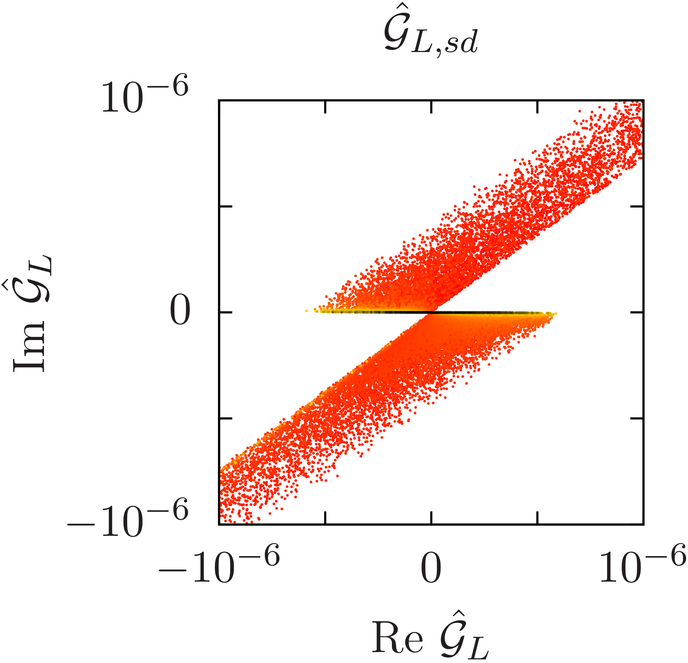
Refer to caption
Refer to caption
Refer to caption
Refer to caption
Refer to caption
Refer to caption
Figure 8: The couplings of the lightest flavour gauge boson to the down-type SM quarks.
Refer to caption
Refer to caption
Refer to caption
Refer to caption
Refer to caption
Refer to caption
Figure 9: The couplings of the lightest flavour gauge boson to the up-type SM quarks.

As an example, we report in fig.ย 8 and 9 the couplings of the lightest gauge boson to the light down- and up-type quarks for the exclusive ๐‘ฝ๐’–โ€‹๐’ƒsubscript๐‘ฝ๐’–๐’ƒV_{ub} case and scattering on all the parameters of the model. The colour-coding corresponds to the mass splitting of the lightest to the next-to-lightest flavour gauge boson mass. Namely, red points correspond to large splitting while black points to degeneracy, yellow to intermediate splitting. We observe that the flavour-violating couplings with the last (first) two generations are in general the largest (smallest) ones. This is related to the sequential breaking of the flavour symmetry encoded into hierarchical structure of the flavon VEVs.

References

  • [1] F.ย Feruglio, C.ย Hagedorn, Y.ย Lin, and L.ย Merlo, Lepton Flavour Violation in a Supersymmetric Model with ๐€๐Ÿ’subscript๐€4A_{4} Flavour Symmetry, Nucl. Phys. B832 (2010) 251โ€“288, arXiv:0911.3874.
  • [2] L.ย Merlo, S.ย Rigolin, and B.ย Zaldivar, Flavour Violation in a Supersymmetric ๐“โ€ฒsuperscript๐“bold-โ€ฒT^{\prime} Model, JHEP 11 (2011) 047, arXiv:1108.1795.
  • [3] R.ย S. Chivukula and H.ย Georgi, Composite Technicolor Standard Model, Phys. Lett. B188 (1987) 99.
  • [4] L.ย J. Hall and L.ย Randall, Weak Scale Effective Supersymmetry, Phys. Rev. Lett. 65 (1990) 2939โ€“2942.
  • [5] M.ย Ciuchini, G.ย Degrassi, P.ย Gambino, and G.ย F. Giudice, Next-To-Leading (QCD) Corrections to ๐ยฏโ†’๐—๐ฌโ€‹๐›„bold-โ†’bold-ยฏ๐subscript๐—๐ฌ๐›„\bar{B}\to X_{s}\gamma in Supersymmetry, Nucl. Phys. B534 (1998) 3โ€“20, hep-ph/9806308.
  • [6] A.ย J. Buras, P.ย Gambino, M.ย Gorbahn, S.ย Jager, and L.ย Silvestrini, Universal Unitarity Triangle and Physics Beyond the Standard Model, Phys. Lett. B500 (2001) 161โ€“167, hep-ph/0007085.
  • [7] G.ย Isidori, Y.ย Nir, and G.ย Perez, Flavor Physics Constraints for Physics Beyond the Standard Model, Ann. Rev. Nucl. Part. Sci. 60 (2010) 355, arXiv:1002.0900.
  • [8] G.ย Dโ€™Ambrosio, G.ย F. Giudice, G.ย Isidori, and A.ย Strumia, Minimal Flavour Violation: an Effective Field Theory Approach, Nucl. Phys. B645 (2002) 155โ€“187, hep-ph/0207036.
  • [9] V.ย Cirigliano, B.ย Grinstein, G.ย Isidori, and M.ย B. Wise, Minimal flavor violation in the lepton sector, Nucl. Phys. B728 (2005) 121โ€“134, hep-ph/0507001.
  • [10] S.ย Davidson and F.ย Palorini, Various Definitions of Minimal Flavour Violation for Leptons, Phys. Lett. B642 (2006) 72โ€“80, hep-ph/0607329.
  • [11] R.ย Alonso, G.ย Isidori, L.ย Merlo, L.ย A. Munoz, and E.ย Nardi, Minimal Flavour Violation Extensions of the Seesaw, JHEP 06 (2011) 037, arXiv:1103.5461.
  • [12] B.ย Grinstein, M.ย Redi, and G.ย Villadoro, Low Scale Flavor Gauge Symmetries, JHEP 11 (2010) 067, arXiv:1009.2049.
  • [13] T.ย Feldmann, See-Saw Masses for Quarks and Leptons in ๐’โ€‹๐”โ€‹(๐Ÿ“)๐’๐”5SU(5), JHEP 04 (2011) 043, arXiv:1010.2116.
  • [14] D.ย Guadagnoli, R.ย N. Mohapatra, and I.ย Sung, Gauged Flavor Group with Left-Right Symmetry, JHEP 04 (2011) 093, arXiv:1103.4170.
  • [15] T.ย Feldmann, M.ย Jung, and T.ย Mannel, Sequential Flavour Symmetry Breaking, Phys. Rev. D80 (2009) 033003, arXiv:0906.1523.
  • [16] R.ย Alonso, M.ย B. Gavela, L.ย Merlo, and S.ย Rigolin, On the Scalar Potential of Minimal Flavour Violation, JHEP 07 (2011) 012, arXiv:1103.2915.
  • [17] A.ย J. Buras, L.ย Merlo, and E.ย Stamou, The Impact of Flavour Changing Neutral Gauge Bosons on ๐ยฏโ†’๐—๐ฌโ€‹๐›„bold-โ†’bold-ยฏ๐subscript๐—๐ฌ๐›„\bar{B}\to X_{s}\gamma, JHEP 1108 (2011) 124, arXiv:1105.5146.
  • [18] A.ย J. Buras, M.ย Misiak, and J.ย Urban, Two-Loop QCD Anomalous Dimensions of Flavour-Changing Four-Quark Operators Within and Beyond the Standard Model, Nucl. Phys. B586 (2000) 397โ€“426, hep-ph/0005183.
  • [19] A.ย J. Buras, S.ย Jager, and J.ย Urban, Master Formulae for ๐šซ๐…=๐Ÿsubscript๐šซ๐…2\Delta_{F}=2 NLO-QCD Factors in the Standard Model and Beyond, Nucl. Phys. B605 (2001) 600โ€“624, hep-ph/0102316.
  • [20] R.ย Babich et.ย al., ๐‘ฒ๐ŸŽโˆ’๐‘ฒยฏ๐ŸŽsuperscript๐‘ฒ0superscriptbold-ยฏ๐‘ฒ0K^{0}-\bar{K}^{0} Mixing Beyond the Standard Model and CP-Violating Electroweak Penguins in Quenched QCD with Exact Chiral Symmetry, Phys. Rev. D74 (2006) 073009, hep-lat/0605016.
  • [21] D.ย Becirevic, V.ย Gimenez, G.ย Martinelli, M.ย Papinutto, and J.ย Reyes, B-Parameters of the Complete Set of Matrix Elements of ๐šซ๐=๐Ÿsubscript๐šซ๐2\Delta_{B}=2 Operators from the Lattice, JHEP 04 (2002) 025, hep-lat/0110091.
  • [22] A.ย J. Buras and D.ย Guadagnoli, Correlations among New CP Violating Effects in ๐šซโ€‹๐…=๐Ÿ๐šซ๐…2\Delta F=2 Observables, Phys. Rev. D78 (2008) 033005, arXiv:0805.3887.
  • [23] T.ย Blum etย al., The ๐Šโ†’(๐›‘โ€‹๐›‘)๐ˆ=๐Ÿbold-โ†’๐Šsubscript๐›‘๐›‘๐ˆ2K\to(\pi\pi)_{I=2} Decay Amplitude from Lattice QCD, arXiv:1111.1699.
  • [24] A.ย J. Buras, D.ย Guadagnoli, and G.ย Isidori, On ฯต๐Šsubscriptbold-ฯต๐Š\epsilon_{K} Beyond Lowest Order in the Operator Product Expansion, Phys. Lett. B688 (2010) 309โ€“313, arXiv:1002.3612.
  • [25] UTfit Collaboration, M.ย Bona et.ย al., The Utfit Collaboration Report on the Status of the Unitarity Triangle Beyond the Standard Model. I: Model- Independent Analysis and Minimal Flavour Violation, JHEP 03 (2006) 080, hep-ph/0509219.
  • [26] Belle Collaboration, K.ย Ikado et.ย al., Evidence of the Purely Leptonic Decay ๐โˆ’โ†’๐›•โˆ’โ€‹๐›Žยฏ๐›•bold-โ†’superscript๐superscript๐›•subscriptbold-ยฏ๐›Ž๐›•B^{-}\to\tau^{-}\bar{\nu}_{\tau}, Phys. Rev. Lett. 97 (2006) 251802, hep-ex/0604018.
  • [27] G.ย Isidori and P.ย Paradisi, Hints of Large Tan(Beta) in Flavour Physics, Phys. Lett. B639 (2006) 499โ€“507, hep-ph/0605012.
  • [28] D0 Collaboration, V.ย M. Abazov et.ย al., Measurement of the Anomalous Like-Sign Dimuon Charge Asymmetry with 9 Fb-1 of ๐ฉโ€‹๐ฉยฏ๐ฉbold-ยฏ๐ฉp\bar{p} Collisions, Phys. Rev. D84 (2011) 052007, arXiv:1106.6308.
  • [29] A.ย Lenz, Theoretical Status of the CKM Matrix, arXiv:1108.1218.
  • [30] T.ย Inami and C.ย S. Lim, Effects of Superheavy Quarks and Leptons in Low-Energy Weak Processes ๐Š๐‹โ†’๐›โ€‹๐›ยฏbold-โ†’subscript๐Š๐‹๐›bold-ยฏ๐›K_{L}\to\mu\bar{\mu}, ๐Š+โ†’๐›‘+โ€‹๐›Žโ€‹๐›Žยฏbold-โ†’superscript๐Šsuperscript๐›‘๐›Žbold-ยฏ๐›ŽK^{+}\to\pi^{+}\nu\bar{\nu} and ๐Š๐ŸŽโ†”๐Šยฏ๐ŸŽbold-โ†”superscript๐Š0superscriptbold-ยฏ๐Š0K^{0}\leftrightarrow\bar{K}^{0}, Prog. Theor. Phys. 65 (1981) 297.
  • [31] E.ย Lunghi and A.ย Soni, Possible Indications of New Physics in ๐โ€‹(๐ƒ)๐๐ƒB(D)-Mixing and in ๐ฌ๐ข๐งโก(๐Ÿโ€‹๐›ƒ)2๐›ƒ\sin(2\beta) Determinations, Phys. Lett. B666 (2008) 162โ€“165, arXiv:0803.4340.
  • [32] A.ย J. Buras and D.ย Guadagnoli, On the Consistency Between the Observed Amount of CP Violation in the ๐Š๐ŠK- and ๐โ€‹(๐ƒ)๐๐ƒB(D)-Systems Within Minimal Flavor Violation, Phys. Rev. D79 (2009) 053010, arXiv:0901.2056.
  • [33] A.ย Lenz et.ย al., Anatomy of New Physics in ๐โˆ’๐ยฏ๐bold-ยฏ๐B-\bar{B} Mixing, Phys. Rev. D83 (2011) 036004, arXiv:1008.1593.
  • [34] RBC Collaboration, D.ย J. Antonio et.ย al., Neutral Kaon Mixing from 2+1 Flavor Domain Wall QCD, Phys. Rev. Lett. 100 (2008) 032001, hep-ph/0702042.
  • [35] C.ย Aubin, J.ย Laiho, and R.ย S. Vanย de Water, The Neutral kaon mixing parameter B(K) from unquenched mixed-action lattice QCD, Phys.Rev. D81 (2010) 014507, arXiv:0905.3947.
  • [36] J.ย Laiho, E.ย Lunghi, and R.ย S. Vanย de Water, Lattice QCD Inputs to the CKM Unitarity Triangle Analysis, Phys. Rev. D81 (2010) 034503, arXiv:0910.2928.
  • [37] T.ย Bae, Y.-C. Jang, C.ย Jung, H.-J. Kim, J.ย Kim, et.ย al., ๐‘ฉ๐‘ฒsubscript๐‘ฉ๐‘ฒB_{K} using HYP-smeared staggered fermions in ๐๐Ÿ=๐Ÿ+๐Ÿsubscript๐๐Ÿ21N_{f}=2+1 unquenched QCD, Phys.Rev. D82 (2010) 114509, arXiv:1008.5179.
  • [38] ETM Collaboration Collaboration, M.ย Constantinou et.ย al., ๐‘ฉ๐‘ฒsubscript๐‘ฉ๐‘ฒB_{K}-parameter from ๐๐Ÿsubscript๐๐ŸN_{f} = 2 twisted mass lattice QCD, Phys.Rev. D83 (2011) 014505, arXiv:1009.5606.
  • [39] Y.ย Aoki et.ย al., Continuum Limit of ๐๐Šsubscript๐๐ŠB_{K} from 2+1 Flavor Domain Wall QCD, Phys. Rev. D84 (2011) 014503, arXiv:1012.4178.
  • [40] J.ย Brod and M.ย Gorbahn, ฯต๐‘ฒsubscriptbold-italic-ฯต๐‘ฒ\epsilon_{K} at Next-To-Next-To-Leading Order: the Charm-Top- Quark Contribution, Phys. Rev. D82 (2010) 094026, arXiv:1007.0684.
  • [41] J.ย Brod and M.ย Gorbahn, The NNLO Charm-Quark Contribution to ฯต๐Šsubscriptbold-ฯต๐Š\epsilon_{K} and ๐šซโ€‹๐Œ๐Š๐šซsubscript๐Œ๐Š\Delta M_{K}, arXiv:1108.2036.
  • [42] E.ย Lunghi and A.ย Soni, Possible Evidence for the Breakdown of the CKM-Paradigm of CP-Violation, Phys. Lett. B697 (2011) 323โ€“328, arXiv:1010.6069.
  • [43] Particle Data Group Collaboration, K.ย Nakamura et.ย al., Review of Particle Physics, J. Phys. G37 (2010) 075021.
  • [44] K.ย G. Chetyrkin et.ย al., Charm and Bottom Quark Masses: an Update, Phys. Rev. D80 (2009) 074010, arXiv:0907.2110.
  • [45] A.ย J. Buras, M.ย Jamin, and P.ย H. Weisz, Leading and Next-To-Leading QCD Corrections to Epsilon Parameter and ๐๐ŸŽโˆ’๐ยฏ๐ŸŽsuperscript๐0superscriptbold-ยฏ๐0B^{0}-\bar{B}^{0} Mixing in the Presence of a Heavy Top Quark, Nucl. Phys. B347 (1990) 491โ€“536.
  • [46] J.ย Urban, F.ย Krauss, U.ย Jentschura, and G.ย Soff, Next-To-Leading Order QCD Corrections for the ๐๐ŸŽโˆ’๐ยฏ๐ŸŽsuperscript๐0superscriptbold-ยฏ๐0B^{0}-\bar{B}^{0} Mixing with an Extended Higgs Sector, Nucl. Phys. B523 (1998) 40โ€“58, hep-ph/9710245.
  • [47] C.ย McNeile, C.ย T.ย H. Davies, E.ย Follana, K.ย Hornbostel, and G.ย P. Lepage, High-Precision ๐Ÿ๐๐ฌsubscript๐Ÿsubscript๐๐ฌf_{B_{s}} and HQET from Relativistic Lattice QCD, Phys.ย Rev. D85 (2012) 031503, arXiv:1110.4510.
  • [48] For the CDF Collaboration, G.ย Giurgiu, New Measurement of the ๐๐ฌsubscript๐๐ฌB_{s} Mixing Phase at CDF, PoS ICHEP2010 (2010) 236, arXiv:1012.0962.
  • [49] D0 Collaboration, V.ย M. Abazov et.ย al., Measurement of the CP-Violating Phase ฯ•๐ฌ๐‰/๐›™โ€‹ฯ•superscriptsubscriptbold-ฯ•๐ฌ๐‰๐›™bold-ฯ•\phi_{s}^{J/\psi\phi} Using the Flavor-Tagged Decay ๐๐ฌ๐ŸŽโ†’๐‰/๐›™โ€‹ฯ•bold-โ†’superscriptsubscript๐๐ฌ0๐‰๐›™bold-ฯ•B_{s}^{0}\rightarrow J/\psi\phi in 8 Fb-1 of ๐ฉโ€‹๐ฉยฏ๐ฉbold-ยฏ๐ฉp\bar{p} Collisions, Phys.ย Rev. D85 (2012) 032006, arXiv:1109.3166.
  • [50] P.ย Koppenburg โ€‹โ€‹, talk at Physics in Collision 2011, Vancouver, BC, Canada, 28 August-1 September 2011.
  • [51] A.ย J. Buras, Minimal Flavour Violation and Beyond: Towards a Flavour Code for Short Distance Dynamics, Acta Phys. Polon. B41 (2010) 2487โ€“2561, arXiv:1012.1447.
  • [52] M.ย Blanke, A.ย J. Buras, D.ย Guadagnoli, and C.ย Tarantino, Minimal Flavour Violation Waiting for Precise Measurements of ๐šซโ€‹๐Œ๐ฌ๐šซsubscript๐Œ๐ฌ\Delta M_{s}, ๐’๐›™โ€‹ฯ•subscript๐’๐›™bold-ฯ•S_{\psi\phi}, ๐€๐ฌโ€‹๐ฅ๐ฌsubscriptsuperscript๐€๐ฌ๐ฌ๐ฅA^{s}_{sl}, |๐•๐ฎโ€‹๐›|subscript๐•๐ฎ๐›|V_{ub}|, ๐›„๐›„\gamma and ๐๐ฌ,๐๐ŸŽโ†’๐›+โ€‹๐›โˆ’bold-โ†’subscriptsuperscript๐0๐ฌ๐superscript๐›superscript๐›B^{0}_{s,d}\to\mu^{+}\mu^{-}, JHEP 10 (2006) 003, hep-ph/0604057.
  • [53] A.ย J. Buras, M.ย Spranger, and A.ย Weiler, The Impact of Universal Extra Dimensions on the Unitarity Triangle and Rare ๐Š๐ŠK and ๐๐B Decays, Nucl. Phys. B660 (2003) 225โ€“268, hep-ph/0212143.
  • [54] M.ย Blanke and A.ย J. Buras, Lower Bounds on ๐šซโ€‹๐Œ๐ฌ,๐๐šซsubscript๐Œ๐ฌ๐\Delta M_{s,d} from Constrained Minimal Flavour Violation, JHEP 05 (2007) 061, hep-ph/0610037.
  • [55] A.ย J. Buras, A.ย Poschenrieder, M.ย Spranger, and A.ย Weiler, The Impact of Universal Extra Dimensions on ๐ยฏโ†’๐—๐ฌโ€‹๐›„bold-โ†’bold-ยฏ๐subscript๐—๐ฌ๐›„\bar{B}\to X_{s}\gamma, ๐ยฏโ†’๐—๐ฌโ€‹๐ bold-โ†’bold-ยฏ๐subscript๐—๐ฌ๐ \bar{B}\to X_{s}g, ๐ยฏโ€‹๐—๐ฌโ€‹๐›+โ€‹๐›โˆ’bold-ยฏ๐subscript๐—๐ฌsuperscript๐›superscript๐›\bar{B}X_{s}\mu^{+}\mu^{-}, ๐Š๐‹โ†’๐›‘๐ŸŽโ€‹๐ž+โ€‹๐žโˆ’bold-โ†’subscript๐Š๐‹superscript๐›‘0superscript๐žsuperscript๐žK_{L}\to\pi^{0}e^{+}e^{-}, and ฯตโ€ฒ/ฯตsuperscriptbold-ฯตbold-โ€ฒbold-ฯต\epsilon^{\prime}/\epsilon, Nucl. Phys. B678 (2004) 455โ€“490, hep-ph/0306158.
  • [56] A.ย J. Buras, M.ย V. Carlucci, S.ย Gori, and G.ย Isidori, Higgs-Mediated FCNCs: Natural Flavour Conservation Vs. Minimal Flavour Violation, JHEP 10 (2010) 009, arXiv:1005.5310.
  • [57] M.ย Blanke, A.ย J. Buras, K.ย Gemmler, and T.ย Heidsieck, ๐šซโ€‹๐‘ญ=๐Ÿ๐šซ๐‘ญ2\Delta F=2 Observables and ๐ยฏโ†’๐—๐โ€‹๐›„bold-โ†’bold-ยฏ๐subscript๐—๐๐›„\bar{B}\to X_{Q}\gamma Decays in the Left-Right Asymmetric Model: Higgs Particles Striking Back, JHEP 1230 (2012) 024, arXiv:1111.5014.