Numerical evidences of universality and self-similarity in the Forced Logistic Map

Abstract

We explore different families of quasi-periodically Forced Logistic Maps for the existence of universality and self-similarity properties. In the bifurcation diagram of the Logistic Map it is well known that there exist parameter values $s_{n}$ where the $2^{n}$-periodic orbit is superattracting. Moreover these parameter values lay between one period doubling and the next. Under quasi-periodic forcing, the superattracting periodic orbits give birth to two reducibility-loss bifurcations in the two dimensional parameter space of the Forced Logistic Map, both around the points $s_{n}$. In the present work we study numerically the asymptotic behavior of the slopes of these bifurcations with respect to $n$. This study evidences the existence of universality properties and self-similarity of the bifurcation diagram in the parameter space.

Universality and self-similarity properties of uniparametric families of unimodal maps are a well known phenomenon. The paradigmatic example of this phenomenon is the Logistic Map $l_{\alpha}(x)=\alpha x(1-x)$. Given a typical one parametric family of unimodal maps $\{l_{\alpha}\}_{\alpha\in I}$ one observes numerically that there exists a sequence of parameter values $\{d_{n}\}_{n\in\mathbb{N}}\subset I$ such that the attracting periodic orbit of the map undergoes a period doubling bifurcation. Between one period doubling and the next there exists a parameter value $s_{n}$, for which the critical point of $l_{s_{n}}$ is a periodic orbit with period $2^{n}$. One can also observe that

$$\lim_{n\rightarrow\infty}\frac{d_{n}-d_{n-1}}{d_{n+1}-d_{n}}=\lim_{n\rightarrow\infty}\frac{s_{n}-s_{n-1}}{s_{n+1}-s_{n}}=\text{\boldmath$\delta$}=\texttt{ 4.66920...}.$$ (1)

The convergence to this limit $\delta$ (the so-called Feigenbaum constant) indicates a self-similarity on the parameter space of the family. On the other hand, the constant $\delta$ is universal, in the sense that one obtains the same ratio $\delta$ for any family of unimodal maps with a quadratic turning point having a cascade of period doubling bifurcations. In this paper we explore if the same kind of phenomenon can be observed when the one dimensional maps is forced quasi-periodically. The answer is that universality and self-similarity do manifest, but they do it in different manners. Moreover, we show that they occur in a more “restrictive” class of maps, in the sense that the quasi-periodic forcing has to have a very particular form. We provide a theoretical explanation to this phenomenon in [20, 21, 22] (see also [19]).

1 Introduction

In the late seventies, Feigenbaum ([6, 7]) and Coullet and Treser ([24]) proposed at the same time the renormalization operator to explain the universal features observed in the cascade of period doubling bifurcations of the Logistic Map. This explanation was based on the existence of a hyperbolic fixed point of the operator with suitable properties. The first proof of the existence of this point and his hyperbolicity were obtained with numeric assistance [16, 5]. In [23] Sullivan generalized the operator and provided a theoretical proof of the hyperbolicity using complex dynamics. In [17, 4] a nice summary of the one dimensional renormalization theory can be found, up to the date of their respective publication, as well as contributions to this theory.

The kind of maps that we consider are maps in the cylinder where the dynamics on the periodic variable is given by a rigid rotation and the dynamics on the other variable is given by an unimodal one dimensional map plus a small perturbation which depends on both variables. These maps are known as quasi-periodically forced one dimensional maps and they have been extensively studied ([10, 11, 18, 12, 8, 14, 2, 9]) with a focus on the existence of strange non-chaotic attractors.

The paradigmatic example in our case of study is the Forced Logistic Map, which is the map on the cylinder $\mathbb{T}\times\mathbb{R}$ defined as

$$\left.\begin{array}[]{rcl}\bar{\theta}&=&\theta+\omega,\\ \bar{x}&=&\alpha x(1-x)(1+\varepsilon\cos(2\pi\theta)),\end{array}\right\}$$ (2)

where $(\alpha,\varepsilon)$ are parameters and $\omega$ is a fixed Diophantine number (typically it will be the golden mean). This family has interest not only for phenomena related with the existence of strange non-chaotic attractors ([11, 18, 8]) but also as a toy-model for the truncation of period doubling bifurcation cascade ([15, 13]). The term “truncation of the period doubling bifurcation cascade” refers to the fact that, when one fixes $\varepsilon$ and let $\alpha$ grow, the attracting set of the map undergoes only a finite number of period doubling bifurcations before exhibiting a chaotic behavior. This differs from the one dimensional case, where the number of period doubling bifurcations before chaos is infinite.

In [13] we studied the truncation of the period doubling cascade for the map (2). We observed that the reducibility of the attracting set plays a crucial role. We computed bifurcation diagrams in terms of the dynamics of the attracting set, taking into account different properties, as the Lyapunov exponent and, in the case of having a periodic invariant curve, its period and its reducibility. One of these bifurcation diagrams is reproduced in Figure 1 (see Table 1 for the label of every color).

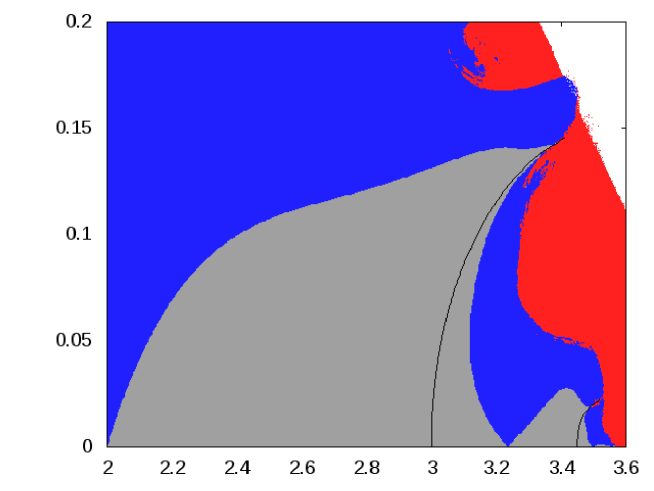
Figure 1: Diagram of the parameter space of the map (2) for $\omega=\frac{\sqrt{5}-1}{2}$. The axis correspond to the parameters $\alpha$ (horizontal) and $\varepsilon$ (vertical). For the correspondence of each color with the properties of the attractor see Table 1. The black lines represent the period doubling bifurcations from period one to two (left) and two to four (right).

Color		Dynamics of the attractor
Black		Invariant curve with zero Lyapunov exponent
Red		Chaotic attractor
Blue		Non-chaotic non-reducible attractor
Grey		Non-chaotic reducible attractor
White		No attractor (divergence to $-\infty$)

Table 1: Color coding for the Figure 1.

Let $d_{n}$ be the parameter value where the attracting periodic orbit of the one dimensional map doubles from period $2^{n}$ to period $2^{n+1}$. Figure 1 reveals that from every parameter $(\alpha,\varepsilon)=(d_{n},0)$ of the map (2) it is born a period doubling bifurcation curve of the attracting set. Let $s_{n}$ be the parameter value where the critical point of the (non-forced) one dimensional family is periodic with period $2^{n}$. In the case of analytic maps in the cylinder, the reducibility loss of an invariant curve can be characterized as a bifurcation, for more details see definition 2.3 in [13]. Figure 1 also reveals that from every parameter value $(\alpha,\varepsilon)=(s_{n},0)$ two curves of reducibility loss are born. These curves correspond to a reducibility-loss and “reducibility-recovery” bifurcations of the $2^{n}$-periodic invariant curve. In [20] we prove, under suitable hypothesis, that these curves exist. In Figure 1 we can observe that the period doubling bifurcation curve born around $(d_{n},0)$ is confined by one of the reducibility loss bifurcation curves born around $(s_{n},0)$ and another one born around $(s_{n+1},0)$.

In this paper we approximate numerically slopes of the reducibility loss bifurcations curves described above and use them to explore for the existence of universality and self-similarity properties within the quasi-periodic one dimensional maps. A posteriori we know that the self-similarity properties exists between the bifurcation diagrams of the map (2) for different values of $\omega$. For a better presentation of the concept, let us start the discussion looking for self-similarity withing the bifurcation diagram of the map (2) with $\omega$ fixed.

2 Description of the computations

Consider the sequence of values $s_{n}$ for which the Logistic Map has a superstable periodic orbit as before. In Figure 1 we can observe how the two curves (namely $S_{n}^{-}$ and $S_{n}^{+}$) that are born at the parameter values $(\alpha,\varepsilon)=(s_{n},0)$ define a region of non-reducibility around this point. Assume that each of these curves correspond to reducibility-loss bifurcations and they can be written locally with $\alpha$ as a graph of $\varepsilon$ (in [20] we give concrete conditions under which this is true). In other words, there exist a neighborhood $U_{n}$ of $s_{n}$, interval $I=[0,\rho)$ and functions $\alpha:I\rightarrow\mathbb{R}$ and $\beta:I\rightarrow\mathbb{R}$ such that $S^{-}_{n}\cap U=\{(\alpha_{n}(\varepsilon),\varepsilon)|\thinspace\varepsilon\in I\}$ and $S^{+}_{n}\cap U=\{(\beta_{n}(\varepsilon),\varepsilon)|\thinspace\varepsilon\in I\}$.

Assume that the functions $\alpha_{n}(\varepsilon)$ and $\beta_{n}(\varepsilon)$ are written at first order as

$$\alpha_{n}(\varepsilon)=s_{n}+\alpha^{\prime}_{n}\varepsilon+o(\varepsilon),\text{ and }\beta_{n}(\varepsilon)=s_{n}+\beta^{\prime}_{n}\varepsilon+o(\varepsilon).$$

Let $s^{*}$ be the limit of the parameter values $s_{n}$. The self-similarity in the bifurcation diagram of the Logistic Map is manifested in the following way. One observes that $s_{n}-s^{*}\approx\delta(s_{n+1}-s^{*})$. In terms of the parameter space this corresponds to the fact that the affine map $L(\alpha)=\delta(\alpha-s^{*})+s^{*}$ sends (approximately) the point $s_{n}$ to $s_{n-1}$. We would like to find an analog self-similarity in the parameter space of the Forced Logistic Map (2). We can use the curves $S^{\pm}_{n}$ to detect this self-similarity. Therefore we look for an affine map of the kind

$$L\left(\begin{array}[]{c}\alpha\\ \varepsilon\end{array}\right)=\left(\begin{array}[]{cc}\delta_{0}&0\\ 0&\delta_{1}\end{array}\right)\left(\begin{array}[]{c}\alpha-s^{*}\\ \varepsilon\end{array}\right)+\left(\begin{array}[]{c}s^{*}\\ 0\end{array}\right),$$ (3)

such that it maps the curves $S^{-}_{n}$ to $S^{-}_{n-1}$ (and respectively $S^{+}_{n}$ to $S^{+}_{n-1}$). If we impose these conditions to the local parameterization (around $s_{i}$) of the curves considered above then we get

$$\left(\begin{array}[]{c}\alpha_{n-1}+\alpha_{n-1}^{\prime}t+o(t)\\ t\end{array}\right)=\left(\begin{array}[]{cc}\delta_{0}&0\\ 0&\delta_{1}\end{array}\right)\left(\begin{array}[]{c}\alpha_{n}+\alpha_{n}^{\prime}s+o(s)-s^{*}\\ s\end{array}\right)+\left(\begin{array}[]{c}s^{*}\\ 0\end{array}\right),$$

for any $t$ and $s$. Then, replacing $s=t/\delta_{1}$ in the first coordinate and equating terms in the order of $t$, we obtain

$$\left\{\begin{array}[]{rcl}\alpha_{n}&=&\delta_{0}\alpha_{n-1}+(1-\delta_{0})s^{*}\\ \alpha^{\prime}_{n}&=&\frac{\delta_{0}}{\delta_{1}}\alpha^{\prime}_{n+1}.\end{array}\right.$$

Using these two equations we have that the value $\delta_{1}$ can be estimated as $\delta_{1}\approx\delta_{0}\frac{\alpha^{\prime}_{n}}{\alpha^{\prime}_{n-1}}$. For $\delta_{0}$ we recover the estimation $\delta_{0}\approx\frac{\alpha_{n}-\alpha_{n-1}}{\alpha_{n-1}-\alpha_{n-2}}$, which converges to the Feigenbaum constant $\delta$. Therefore we replace $\delta_{0}$ by $\delta$ in the estimation of $\delta_{1}$, obtaining $\delta_{1}\approx\text{\boldmath$\delta$}\frac{\alpha^{\prime}_{n}}{\alpha^{\prime}_{n-1}}$.

To obtain a numerical approximation of the values $\alpha^{\prime}_{n}$ we have computed points in the curve $(\alpha_{n}(\varepsilon),\varepsilon)\in S^{-}_{n}$ for small values of $\varepsilon=2^{-k}h_{n}$ for different values of $k=1,2,...,M$ and $h_{n}$ a prescribed value depending on $n$ (which have been decreased when we increased $n$). Then, we have used this set of points to estimate the value $\alpha_{n}^{\prime}\approx\frac{\alpha_{n}(2^{-k}h_{n})-\alpha_{n}(0)}{2^{-k}h_{n}}$, and we did three steps of extrapolation to improve the accuracy of the results. We have also considered consecutive approximations to estimate the accuracy of the results. These computations have been done with quadruple precision (using the library [1]).

To compute each of the values $(\alpha_{n}(\varepsilon),\varepsilon)$ with good accuracy we have used the following procedure. We have computed the $2^{n}$ periodic invariant curve of the system approximating it by its Fourier expansion. We use the same method described in Section 3.2.1 in [13] (originally from [3]) to continue the zero Lyapunov exponent but tuned to continue the reducibility loss bifurcation curve. To continue this curve we use the characterization of the reducibility loss bifurcation given by Definition 2.3 in [13].

3 Description of the results

The values of $\alpha^{\prime}_{n}$ actually depend on $\omega$ (the rotation number of the system). Hence, from now on, we write $\alpha^{\prime}_{n}=\alpha^{\prime}_{n}(\omega)$. The estimated values of $\alpha^{\prime}_{n}(\omega)$ for the family (2) when $\omega=\frac{\sqrt{5}-1}{2}$ are shown in Table 4. We have included the ratios $\alpha^{\prime}_{n}(\omega)/\alpha^{\prime}_{n-1}(\omega)$ in the third column of the table. The value $\epsilon_{a}$ in the fourth column corresponds to the estimated accuracy (in absolute terms) for the value of $\alpha_{n}^{\prime}$. In Tables 4 and 4 we included the same values for $\omega=2\frac{\sqrt{5}-1}{2}$ and $\omega=4\frac{\sqrt{5}-1}{2}$.

We have computed the approximate value of $\beta^{\prime}_{i}$ for the same values of $\omega$, but in all cases the value obtained has been equal (in the accuracy of the computations) to $-\alpha^{\prime}_{i}$. Because of that these results will be omitted of the discussion.

We can observe in Tables 4, 4 and 4 that the ratios $\alpha^{\prime}_{i}(\omega)/\alpha^{\prime}_{i-1}(\omega)$ do not converge to a constant. Therefore (a priory) it seems that there are no self-similarity of the bifurcation diagram. In fact, we will see in Section 3.2 that one has to do a more subtle analysis to uncover the self-similarity properties of the family.

3.1 Universality of the ratio sequence

A remarkable fact is that the ratios $\alpha^{\prime}_{i}(\omega)/\alpha^{\prime}_{i-1}(\omega)$ on the third column of Table 4 are approximately the same values on the third column of Table 4, but shifted on the index value $n$ by one position. Actually, the bigger is $n$ the closer are the values. The same phenomenon can be observed in Tables 4 and 4.

Let us introduce some additional notation to follow with the analysis of this phenomenon. Consider $F$ a quasi-periodic forced map as follows,

$$\begin{array}[]{rccc}F:&\mathbb{T}\times R&\rightarrow&\mathbb{T}\times R\\ &\left(\begin{array}[]{c}\theta\\ x\end{array}\right)&\mapsto&\left(\begin{array}[]{c}\theta+\omega\\ f(\theta,x)\end{array}\right),\end{array}$$ (4)

where $f$ is a $C^{r}$ map and $\omega$ an irrational number. This map $F$ can be identified with a pair $(\omega,f)\in\mathbb{T}\cap(\mathbb{R}\setminus\mathbb{Q})\times C^{r}(\mathbb{T}\times\mathbb{R},\mathbb{R})$. Consider $\alpha_{n}^{\prime}(\omega)$ the slope of the reducibility-loss bifurcation introduced before. Nothing ensures yet their existence for a general map $F=(\omega,f)$, but whenever they exist they can be thought also depending, not only on $\omega$, but also on the function $f$ of the map $F$ considered [25]. In other words we consider $\alpha_{n}^{\prime}(\omega)=\alpha_{n}^{\prime}(\omega,f)$.

Given two sequences $\{r_{i}\}_{i\in\mathbb{Z}_{+}}$ and $\{s_{i}\}_{i\in\mathbb{Z}_{+}}$ of real numbers, we say that they are asymptotically equivalent [26] if there exists $0<\rho<1$ and $K_{0}$ such that

$$|r_{i}-s_{i}|\leq K_{0}\rho^{i}\quad\forall i\in\mathbb{Z}_{+}.$$

We denote this equivalence relation simply by $s_{i}\sim r_{i}$.

Now we can resume the discussion on the phenomenon observed on Tables 4, 4 and 4. Our numerical computations suggest that

$$\frac{\alpha_{i}^{\prime}(\omega,f)}{\alpha_{i-1}^{\prime}(\omega,f)}\sim\frac{\alpha_{i-1}^{\prime}(2\omega,f)}{\alpha_{i-2}^{\prime}(2\omega,f)}.$$ (5)

Consider two different values $\omega_{0}$ and $\omega_{1}$ such that $2\omega_{0}=2\omega_{1}(\mod 1)$ . If equation (5) is true, then $\alpha_{i}^{\prime}(\omega_{0},f)/\alpha_{i-1}^{\prime}(\omega_{0},f)$ and $\alpha_{i}^{\prime}(\omega_{1},f)/\alpha_{i-1}^{\prime}(\omega_{1},f)$ should be asymptotically equivalent. This can be checked numerically. In Table 7 we have recomputed the same values of Table 4 but this time for $\omega=\frac{\sqrt{5}}{2}$ (and $f$ the function associated to the map (2) as before). Again the results obtained show asymptotic equivalence.

n	$\alpha_{n}^{\prime}(\omega)$	$\alpha_{n}^{\prime}(\omega)/\alpha_{n-1}^{\prime}(\omega)$	$\epsilon_{a}$
0	-2.0000000000e+00	- - -	3.0e-15
1	-5.8329149229e+00	2.9164574614e+00	1.5e-14
2	-8.4942599432e+00	1.4562633015e+00	8.4e-13
3	-1.6351279467e+01	1.9249798777e+00	7.4e-15
4	-1.1252460775e+01	6.8817004793e-01	3.0e-14
5	-1.2243326651e+01	1.0880577054e+00	1.6e-13
6	-1.8079693906e+01	1.4766978307e+00	1.6e-11
7	-3.4735234067e+01	1.9212291009e+00	2.0e-12
8	-2.9583312211e+01	8.5168023205e-01	2.1e-12
9	-4.1569457725e+01	1.4051657715e+00	4.2e-10
10	-7.8965495522e+01	1.8996036957e+00	9.1e-11
11	-7.4500733455e+01	9.4345932945e-01	8.1e-10

Table 2: Approximate values of $\alpha_{n}^{\prime}(\omega)$ for the map (2) for $\omega=\frac{\sqrt{5}-1}{2}$.

n	$\alpha_{n}^{\prime}(\omega)$	$\alpha_{n}^{\prime}(\omega)/\alpha_{n-1}^{\prime}(\omega)$	$\epsilon_{a}$
0	-2.0000000000e+00	- - -	4.1e-16
1	-4.7793787548e+00	2.3896893774e+00	9.2e-14
2	-9.9177338359e+00	2.0751094117e+00	8.0e-16
3	-6.9333908531e+00	6.9909023249e-01	4.3e-15
4	-7.5678156188e+00	1.0915028129e+00	2.4e-14
5	-1.1183261803e+01	1.4777397292e+00	2.3e-12
6	-2.1488744556e+01	1.9215095679e+00	3.0e-13
7	-1.8302110429e+01	8.5170682641e-01	3.1e-13
8	-2.5717669657e+01	1.4051750893e+00	6.1e-11
9	-4.8853450105e+01	1.8996064090e+00	2.6e-11
10	-4.6091257360e+01	9.4345961772e-01	1.2e-10
11	-7.1498516059e+01	1.5512381339e+00	4.1e-09

Table 3: Approximate values of $\alpha_{n}^{\prime}(\omega)$ for the map (2) for $\omega=2\frac{\sqrt{5}-1}{2}$.

n	$\alpha_{n}^{\prime}(\omega)$	$\alpha_{n}^{\prime}(\omega)/\alpha_{n-1}^{\prime}(\omega)$	$\epsilon_{a}$
0	-2.0000000000e+00	- - -	5.3e-15
1	-6.1135714539e+00	3.0567857269e+00	4.0e-17
2	-4.6432689399e+00	7.5950186809e-01	8.8e-16
3	-5.1662366620e+00	1.1126292121e+00	5.4e-15
4	-7.6637702641e+00	1.4834338350e+00	5.2e-13
5	-1.4738755184e+01	1.9231728870e+00	6.7e-14
6	-1.2555429245e+01	8.5186497017e-01	6.9e-14
7	-1.7643286059e+01	1.4052316105e+00	1.3e-11
8	-3.3515585777e+01	1.8996226477e+00	5.8e-12
9	-3.1620659727e+01	9.4346134772e-01	2.6e-11
10	-4.9051192417e+01	1.5512387420e+00	9.0e-10
11	-9.2911119039e+01	1.8941663691e+00	5.6e-12

Table 4: Approximate values of $\alpha_{n}^{\prime}(\omega)$ for the map (2) for $\omega=4\frac{\sqrt{5}-1}{2}$.

n	$\alpha_{n}^{\prime}(\omega)$	$\alpha_{n}^{\prime}(\omega)/\alpha_{n-1}^{\prime}(\omega)$	$\epsilon_{a}$
0	-2.0000000000e+00	- - -	5.3e-17
1	-3.7459592187e+00	1.8729796094e+00	3.6e-15
2	-6.1798012892e+00	1.6497246575e+00	2.4e-13
3	-1.2170152952e+01	1.9693437350e+00	2.1e-15
4	-8.4095313813e+00	6.9099635922e-01	9.5e-15
5	-9.1576001570e+00	1.0889548706e+00	5.2e-14
6	-1.3525371011e+01	1.4769558377e+00	5.0e-12
7	-2.5986306241e+01	1.9213008072e+00	6.5e-13
8	-2.2132200091e+01	8.5168703416e-01	6.6e-13
9	-3.1099463199e+01	1.4051681745e+00	1.3e-10
10	-5.9076676864e+01	1.8996043914e+00	5.6e-11
11	-5.5736446311e+01	9.4345940345e-01	2.5e-10

Table 5: Approximate values of $\alpha_{n}^{\prime}(\omega)$ for the map (2) for $\omega=\frac{\sqrt{5}}{2}$.

n	$\alpha_{n}^{\prime}(\omega)$	$\alpha_{n}^{\prime}(\omega)/\alpha_{n-1}^{\prime}(\omega)$	$\epsilon_{a}$
0	-4.0000000000e+00	- - -	2.7e-14
1	-8.1607837043e+00	2.0401959261e+00	5.1e-14
2	-1.1166652707e+01	1.3683309241e+00	2.4e-12
3	-2.1221554117e+01	1.9004400578e+00	2.1e-14
4	-1.4564213015e+01	6.8629342294e-01	8.6e-14
5	-1.5837452605e+01	1.0874224778e+00	4.6e-13
6	-2.3384207858e+01	1.4765132021e+00	4.5e-11
7	-4.4925217655e+01	1.9211776567e+00	5.8e-12
8	-3.8261700375e+01	8.5167534788e-01	5.9e-12
9	-5.3763965691e+01	1.4051640456e+00	1.1e-09
10	-1.0213020106e+02	1.8996031960e+00	1.1e-10
11	-9.6355685578e+01	9.4345927630e-01	2.3e-09

Table 6: Approximate values of $\alpha_{n}^{\prime}$ for the map (7) for $\omega=\frac{\sqrt{5}-1}{2}$.

n	$\alpha_{n}^{\prime}(\omega)$	$\alpha_{n}^{\prime}(\omega)/\alpha_{n-1}^{\prime}(\omega)$	$\epsilon_{a}$
0	-4.0000000000e+00	- - -	3.8e-15
1	-6.2417012728e+00	1.5604253182e+00	2.4e-13
2	-1.2036825830e+01	1.9284527253e+00	2.1e-15
3	-8.2891818940e+00	6.8865180997e-01	9.0e-15
4	-9.0187641307e+00	1.0880161934e+00	4.9e-14
5	-1.3318271659e+01	1.4767291245e+00	4.7e-12
6	-2.5587438370e+01	1.9212281462e+00	6.1e-13
7	-2.1792312360e+01	8.5168011135e-01	6.2e-13
8	-3.0621808757e+01	1.4051656497e+00	1.2e-10
9	-5.8169300479e+01	1.8996036760e+00	5.2e-11
10	-5.4880369083e+01	9.4345932701e-01	2.3e-10
11	-8.5132515708e+01	1.5512380316e+00	8.2e-09

Table 7: Approximate values of $\alpha_{n}^{\prime}$ for the map (7) for $\omega=2\frac{\sqrt{5}-1}{2}$.

Given $F$ a skew product map like (4), let $F^{2}$ denote the map composed with itself. Concretely, the map $F^{2}$ is given as $F^{2}(\theta,x)=(\theta+2\omega,f(\theta+\omega,f(\theta,x)))$. To simplify the notation, let us denote by $f^{2}$ the map defined as $f^{2}(\theta,x):=f(\theta+\omega,f(\theta,x))$. Then we have that the map $F^{2}$ corresponds to the pair $(2\omega,f^{2})$. Moreover we have that the $2^{k}$ periodic curves are $2^{k-1}$ periodic curves of the map $F^{2}$, therefore $\alpha_{i}^{\prime}(\omega,f)=\alpha_{i-1}^{\prime}(2\omega,f^{2})$. Hence the relation given by (5) can be rewritten as

$$\frac{\alpha_{i}^{\prime}(2\omega,f^{2})}{\alpha_{i-1}^{\prime}(2\omega,f^{2})}\sim\frac{\alpha_{i}^{\prime}(2\omega,f)}{\alpha_{i-1}^{\prime}(2\omega,f)}.$$ (6)

Now we have that the relation given by (5) can be explained as a consequence of a much more general phenomenon. We believe that the sequence $\frac{\alpha_{i}^{\prime}(2\omega,f)}{\alpha_{i-1}^{\prime}(2\omega,f)}$ is (asymptotically) universal, in the sense that it does not depend on the map $f$. This would imply (6) and consequently (5).

To check the universality of the sequence, we consider the following map,

$$\left.\begin{array}[]{rcl}\bar{\theta}&=&\theta+\omega,\\ \bar{x}&=&\alpha x(1-x)+\varepsilon\cos(2\pi\theta).\end{array}\right\}$$ (7)

This map is like (2) but with an additive forcing instead of a multiplicative one. In the literature, sometimes (2) is referred as the Driven Logistic Map and (7) is referred as the Forced Logistic Map. We do not do this distinction in this paper and we consider both as two different versions of the Forced Logistic Map.

Note that both maps are in the class of quasi-periodically forced one dimensional unimodal maps, with a quasi-periodic forcing of the type $h(x)\cos(2\pi\theta)$, where $h$ is a function of one variable. This is certainly a very restrictive class of maps. In Section 3.3 we explore what happens when the quasi-periodic forcing is not of this form.

We have computed the slopes $\alpha_{n}^{\prime}(\omega)$, the associated ratios $\alpha_{n}^{\prime}(\omega)/\alpha_{n-1}^{\prime}(\omega)$ and the estimation of the accuracy for the family (7) as we did before for the family (2). The results are shown in Table 7 for $\omega=\frac{\sqrt{5}-1}{2}$ and Table 7 for $\omega=2\frac{\sqrt{5}-1}{2}$.

Now we can compare the sequences $\alpha_{i}^{\prime}(\omega_{0})/\alpha_{i-1}^{\prime}(\omega_{0})$ in Table 4 (respectively 4) with the ones of Table 7 (respectively 7). Again we can observe that both sequences have an equivalent asymptotic behavior for equal values of $\omega$. This agrees with the conjectured universal behavior.

3.2 Self-similarity of the bifurcation diagram

n	$\delta_{1,n}(\omega_{0})$	$\delta_{1,n}-\delta_{1,n-1}$	$\delta_{1,n}(\omega_{0})$	$\delta_{1,n}-\delta_{1,n-1}$
1	1.36175279e+01	- - -	1.11579415e+01	- - -
2	8.29844510e+00	-5.3e+00	7.57460662e+00	-3.6e+00
3	7.69807112e+00	-6.0e-01	6.97211386e+00	-6.0e-01
4	7.57782290e+00	-1.2e-01	6.83972864e+00	-1.3e-01
5	7.55390503e+00	-2.4e-02	6.81347460e+00	-2.6e-02
6	7.54857906e+00	-5.3e-03	6.80758174e+00	-5.9e-03
7	7.54747726e+00	-1.1e-03	6.80631795e+00	-1.3e-03
8	7.54724159e+00	-2.4e-04	6.80604419e+00	-2.7e-04
9	7.54719154e+00	-5.0e-05	6.80598601e+00	-5.8e-05
10	7.54718076e+00	-1.1e-05	6.80597353e+00	-1.2e-05
11	7.54717846e+00	-2.3e-06	6.80597086e+00	-2.7e-06

Table 8: Estimations of the value $\delta_{1,n}=\delta_{1,n}(\omega)=\text{\boldmath$\delta$}\frac{\alpha_{n}^{\prime}(\omega_{0})}{\alpha_{n-1}^{\prime}(2\omega_{0})}$ for $\omega_{0}=\frac{\sqrt{5}-1}{2}$ on the left and $\omega_{1}=2\frac{\sqrt{5}-1}{2}$ on the right.

n	$\delta_{1,n}(\omega_{0})$	$\delta_{1,n}-\delta_{1,n-1}$
1	9.52608610e+00	- - -
2	8.35338804e+00	-1.2e+00
3	8.23204689e+00	-1.2e-01
4	8.20385506e+00	-2.8e-02
5	8.19937833e+00	-4.5e-03
6	8.19817945e+00	-1.2e-03
7	8.19796400e+00	-2.2e-04
8	8.19791815e+00	-4.6e-05
9	8.19790879e+00	-9.4e-06
10	8.19790672e+00	-2.1e-06
11	8.19790628e+00	-4.4e-07

Table 9: Estimations of the value $\delta_{1,n}=\delta_{1,n}(\omega)=\text{\boldmath$\delta$}\frac{\alpha_{n}^{\prime}(\omega_{0})}{\alpha_{n-1}^{\prime}(2\omega_{0})}$ for $\omega_{0}=\frac{\sqrt{5}-1}{2}$ for the family (7) with $\omega_{0}=\frac{\sqrt{5}-1}{2}$ .

In order to find self-similarity properties of the parameter space we need to refine our analysis. Given a one dimensional map in the interval $g:I\rightarrow I$, its (doubling) renormalization is defined as $\mathcal{R}(f)=A^{-1}\circ g\circ g\circ A$ with $A$ an affine transformation. Given a q.p. forced map like (4), one might try to define a renormalization for these kind of maps. The most simple choice would be to define its (doubling) renormalization also as $\mathcal{T}(F)=A^{-1}\circ F\circ F\circ A$, with $A$ a suitable affine map. If the map $F$ has rotation number $\omega$, its (doubling) renormalization will have rotation number $2\omega$. This is due to the composition of $F$ with itself when we define its renormalization. This argument become more clear in the rigorous definition of the renormalization operator for quasi-periodically maps done in [20].

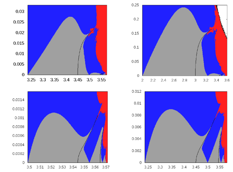
Figure 2: Diagram of the parameter space of the map (2) for $\omega=\frac{\sqrt{5}-1}{2}$ on the left hand side and for $\omega=\sqrt{5}-1$ on the right. See Table 1 for the coding of each color and the text for more details.

Consider the reducibility loss curves $S^{\pm}_{n}$ as in the parameter space of the map (2) (see Section 2). We have that these curves depend on the rotation number (i.e. $S^{\pm}_{n}=S^{\pm}_{n}(\omega)$). Now we can look for self-similarity of the parameter space as in Section 2 but taking into account the doubling of the rotation number. In other words we can look for affine relationship between the bifurcation diagram around $s_{n}$ for $\omega_{0}$ and the bifurcation diagram around $s_{n-1}$ for $2\omega_{0}$. Consider an affine map like (3), but such that it maps the curves $S^{-}_{i}(\omega)$ to $S^{-}_{i-1}(2\omega)$ (and respectively $S^{+}_{i}(\omega)$ to $S^{+}_{i-1}(2\omega)$). Redoing the same computation of Section 2 we have that if there exists an affine relation between the parameters spaces it should be given by $\delta_{1}\approx\text{\boldmath$\delta$}\frac{\alpha_{i}(\omega)}{\alpha_{i-1}(2\omega)}$.

In Table 8 we have estimations of these values for the family (2) for $\omega=\frac{\sqrt{5}-1}{2}$ (left) and $\omega=\sqrt{5}-1$ (right). In Table 9 we have the same estimation for the family (7) and $\omega=\frac{\sqrt{5}-1}{2}$. In all cases the sequence converges to a concrete value. This convergence means that there exists an affine relation between the reducibility loss bifurcation curves around the superstable periodic orbits of the uncoupled map. Note that the limit constants obtained in each of these three cases are different one to each other. This indicates that the renormalization factor depends both on the value of $\omega$ taken and the family of maps considered. Therefore the renormalization factor $\delta_{1}$ is not universal.

These evidences of self-similarity are only valid for infinitely small values of the coupling parameter $\varepsilon$. If the self-similarity between families extends to larger values of $\varepsilon$, the bifurcation diagram of the map (2) in a box $I_{1}\times I_{2}$ of the parameters space for a prescribed $\omega=\omega_{0}$ should be approximately the same as the diagram in the box $L(I_{1}\times I_{2})$ for $\omega=2\omega_{0}$, where $L$ is the affine map (3).

In Figure 2 we have a bifurcation diagram of the map (2) analog to the one displayed in Figure 1. The boxes have been selected such that the one in the left is the image of the one in the right through the affine map $L$ given by (3). The value of $\delta_{0}$ has been taken equal to the Feigenbaum constant ($\approx\texttt{4,66920}$) and $\delta_{1}\approx\texttt{7,54718}$ the experimental value obtained in Table 8. The results indicate that self-similarity properties extend to the whole reducibility region around each period doubling bifurcation.

3.3 Non-universality of the ratio sequence under more general conditions

n	$\alpha_{n}^{\prime}(\omega)$	$\alpha_{n}^{\prime}(\omega)/\alpha_{n-1}^{\prime}(\omega)$	$\epsilon_{a}$
0	-4.4000000000e+00	- - -	2.1e-14
1	-8.5708073961e+00	1.9479107718e+00	3.2e-14
2	-1.2367363641e+01	1.4429636637e+00	2.5e-12
3	-2.2002414361e+01	1.7790707058e+00	2.0e-14
4	-1.5466051366e+01	7.0292519321e-01	1.2e-13
5	-1.7124001858e+01	1.1071993396e+00	7.5e-13
6	-2.5233583736e+01	1.4735798293e+00	5.0e-11
7	-4.5526415150e+01	1.8041993411e+00	4.4e-12
8	-4.0793050977e+01	8.9603037802e-01	3.7e-12
9	-5.9579098646e+01	1.4605207804e+00	1.1e-09
10	-1.0695246126e+02	1.7951339260e+00	9.0e-11
11	-1.0464907069e+02	9.7846341692e-01	3.1e-09

Table 10: Approximate values of $\alpha_{n}^{\prime}(\omega)$ of the family (8) for $\omega=\frac{\sqrt{5}-1}{2}$ and $E=10^{-1}$.

n	$\alpha_{n}^{\prime}(\omega)$	$\alpha_{n}^{\prime}(\omega)/\alpha_{n-1}^{\prime}(\omega)$	$\epsilon_{a}$
0	-4.4000000000e+00	- - -	4.2e-15
1	-6.8849393233e+00	1.5647589371e+00	2.6e-13
2	-1.2339134533e+01	1.7921921972e+00	1.9e-15
3	-8.8252833730e+00	7.1522709709e-01	1.0e-14
4	-9.9507316299e+00	1.1275254526e+00	2.6e-14
5	-1.5240261120e+01	1.5315719172e+00	4.9e-12
6	-2.6987715314e+01	1.7708171207e+00	6.9e-13
7	-2.4101506278e+01	8.9305471016e-01	1.0e-12
8	-3.4274713216e+01	1.4220983876e+00	1.4e-10
9	-5.9739968275e+01	1.7429750002e+00	4.0e-11
10	-6.0772668123e+01	1.0172865818e+00	3.5e-10
11	-9.7063373626e+01	1.5971550472e+00	8.3e-09

Table 11: Approximate values of $\alpha_{n}^{\prime}(\omega)$ of the family (8) for $\omega=2\frac{\sqrt{5}-1}{2}$ and $E=10^{-1}$.

n	$\alpha_{n}^{\prime}(\omega)$	$\alpha_{n}^{\prime}(\omega)/\alpha_{n-1}^{\prime}(\omega)$	$\epsilon_{a}$
0	-4.0400000000e+00	- - -	2.6e-14
1	-8.1970065912e+00	2.0289620275e+00	4.9e-14
2	-1.1286613379e+01	1.3769189098e+00	2.4e-12
3	-2.1298993542e+01	1.8871022535e+00	2.1e-14
4	-1.4654396022e+01	6.8803232383e-01	8.9e-14
5	-1.5964802815e+01	1.0894207302e+00	5.0e-13
6	-2.3545880397e+01	1.4748619617e+00	4.5e-11
7	-4.4967877741e+01	1.9097981041e+00	5.6e-12
8	-3.8501241787e+01	8.5619432630e-01	4.8e-12
9	-5.4345411904e+01	1.4115236128e+00	1.1e-09
10	-1.0260055779e+02	1.8879341272e+00	1.0e-10
11	-9.7178352178e+01	9.4715227943e-01	2.3e-09

Table 12: Approximate values of $\alpha_{n}^{\prime}(\omega)$ of the family (8) for $\omega=\frac{\sqrt{5}-1}{2}$ and $E=10^{-2}$.

n	$\alpha_{n}^{\prime}(\omega)$	$\alpha_{n}^{\prime}(\omega)/\alpha_{n-1}^{\prime}(\omega)$	$\epsilon_{a}$
0	-4.0400000000e+00	- - -	3.8e-15
1	-6.2967793362e+00	1.5586087466e+00	2.4e-13
2	-1.2062745707e+01	1.9157008786e+00	2.1e-15
3	-8.3390918858e+00	6.9130959805e-01	9.0e-15
4	-9.1092083960e+00	1.0923501648e+00	4.6e-14
5	-1.3509885744e+01	1.4831020608e+00	4.7e-12
6	-2.5722289496e+01	1.9039605503e+00	6.1e-13
7	-2.2023032848e+01	8.5618478288e-01	6.8e-13
8	-3.0953588852e+01	1.4055098163e+00	1.2e-10
9	-5.8281365651e+01	1.8828629510e+00	5.1e-11
10	-5.5448581611e+01	9.5139468666e-01	2.5e-10
11	-8.6313143445e+01	1.5566339289e+00	8.2e-09

Table 13: Approximate values of $\alpha_{n}^{\prime}(\omega)$ of the family (8) for $\omega=2\frac{\sqrt{5}-1}{2}$ and $E=10^{-2}$.

n	$\alpha_{n}^{\prime}(\omega)$	$\alpha_{n}^{\prime}(\omega)/\alpha_{n-1}^{\prime}(\omega)$	$\epsilon_{a}$
0	-4.0040000000e+00	- - -	2.7e-14
1	-8.1643491058e+00	2.0390482282e+00	5.0e-14
2	-1.1178647202e+01	1.3692024995e+00	2.4e-12
3	-2.1229290655e+01	1.8990930004e+00	2.1e-14
4	-1.4573231305e+01	6.8646812284e-01	8.6e-14
5	-1.5850170411e+01	1.0876222355e+00	4.7e-13
6	-2.3400073191e+01	1.4763294391e+00	4.5e-11
7	-4.4929300750e+01	1.9200495820e+00	5.7e-12
8	-3.8285483755e+01	8.5212730036e-01	5.8e-12
9	-5.3822109356e+01	1.4058098286e+00	1.1e-09
10	-1.0217709608e+02	1.8984223641e+00	1.0e-10
11	-9.6437862923e+01	9.4383053171e-01	2.2e-09

Table 14: Approximate values of $\alpha_{n}^{\prime}(\omega)$ of the family (8) for $\omega=\frac{\sqrt{5}-1}{2}$ and $E=10^{-3}$.

n	$\alpha_{n}^{\prime}(\omega)$	$\alpha_{n}^{\prime}(\omega)/\alpha_{n-1}^{\prime}(\omega)$	$\epsilon_{a}$
0	-4.0040000000e+00	- - -	3.7e-15
1	-6.2470810635e+00	1.5602100558e+00	2.4e-13
2	-1.2039370639e+01	1.9271993618e+00	2.1e-15
3	-8.2941266770e+00	6.8891696467e-01	9.0e-15
4	-9.0277699390e+00	1.0884533466e+00	4.8e-14
5	-1.3337423899e+01	1.4773774686e+00	4.7e-12
6	-2.5600860673e+01	1.9194756698e+00	6.1e-13
7	-2.1815381589e+01	8.5213469453e-01	6.3e-13
8	-3.0654499563e+01	1.4051782426e+00	1.2e-10
9	-5.8180013759e+01	1.8979273708e+00	5.2e-11
10	-5.4936892373e+01	9.4425712239e-01	2.4e-10
11	-8.5250385421e+01	1.5517875464e+00	8.2e-09

Table 15: Approximate values of $\alpha_{n}^{\prime}(\omega)$ of the family (8) for $\omega=2\frac{\sqrt{5}-1}{2}$ and $E=10^{-3}$.

n $\delta_{1,n}(\omega_{0})$ $\delta_{1,n}-\delta_{1,n-1}$ 1 9.095188 - - - 2 8.387251 -7.1e-01 3 8.325844 -6.1e-02 4 8.182639 -1.4e-01 5 8.035129 -1.5e-01 6 7.730884 -3.0e-01 7 7.876621 1.5e-01 8 7.902866 2.6e-02 9 8.116387 2.1e-01 10 8.359271 2.4e-01 11 8.040253 -3.2e-01 n $\delta_{1,n}(\omega_{0})$ $\delta_{1,n}-\delta_{1,n-1}$ 1 9.473633 - - - 2 8.369274 -1.1e+00 3 8.244333 -1.2e-01 4 8.205249 -3.9e-02 5 8.183245 -2.2e-02 6 8.137779 -4.5e-02 7 8.162729 2.5e-02 8 8.162820 9.1e-05 9 8.197747 3.5e-02 10 8.219826 2.2e-02 11 8.183173 -3.7e-02 n $\delta_{1,n}(\omega_{0})$ $\delta_{1,n}-\delta_{1,n-1}$ 1 9.520727 - - - 2 8.355159 -1.2e+00 3 8.233307 -1.2e-01 4 8.204041 -2.9e-02 5 8.197777 -6.3e-03 6 8.191961 -5.8e-03 7 8.194411 2.4e-03 8 8.194339 -7.1e-05 9 8.198023 3.7e-03 10 8.200161 2.1e-03 11 8.196456 -3.7e-03

Table 16: Estimations of the value $\delta_{1,n}=\delta_{1,n}(\omega)=\text{\boldmath$\delta$}\frac{\alpha_{n}^{\prime}(\omega_{0})}{\alpha_{n-1}^{\prime}(2\omega_{0})}$ for the map (8) (where $\delta$ is the Feigenbaum constant). The different boxes correspond (from left to right) to $E=10^{-1},10^{-2}$ and $10^{-3}$. In all the cases we have taken $\omega=\frac{\sqrt{5}-1}{2}$.

A natural question to ask after the numerical evidences of universality and renormalization reported in the previous sections is “how general are these phenomena?”. In this section we present an example which demonstrates that the universality and the self similarity properties depend on the Fourier expansion of the quasi-periodic forcing. We must say that we designed this example after developing some of the theory presented in [20, 21, 22] and the cited theory provides a theoretical explanation to both behaviors.

Consider the following family,

$$\left.\begin{array}[]{rcl}\bar{\theta}&=&\theta+\omega,\\ \bar{x}&=&\alpha x(1-x)+\varepsilon(\cos(2\pi\theta)+E\cos(4\pi\theta)).\end{array}\right\}$$ (8)

We consider $E$ a fixed value and $\alpha$ and $\varepsilon$ as true parameters, obtaining a two parametric family. Remark that for $E=0$ we recover the family (7) introduced in Section 3.1.

We have done the computation of the values $\alpha_{n}^{\prime}(\omega)$ for the family (8), for $E=10^{-1},10^{-2},10^{-3}$ and $\omega=\frac{\sqrt{5}-1}{2},2\frac{\sqrt{5}-1}{2}$. The results are shown in Tables 12 to 15. To compute the values in the tables we have used the same procedure that we have used for the families (2) and (7) before. In these tables we have also included the estimated values of the ratios $\alpha_{n}^{\prime}(\omega)/\alpha_{n-1}^{\prime}(\omega)$ and the estimated accuracies. In Table 16 we include the ratios $\delta_{1,n}(\omega)=\alpha_{n}^{\prime}(\omega)/\alpha_{n-1}^{\prime}(2\omega)$ and the differences $\delta_{1,n}(\omega)-\delta_{1,n-1}(\omega)$.

In the third column of Tables 12 to 15 we can observe that the sequence of ratios $\alpha_{n}^{\prime}(\omega)/\alpha_{n-1}^{\prime}(\omega)$ ceases to be universal. In other words, the sequence is not asymptotically equivalent to the sequences obtained for the maps (2) and (7) (displayed in Tables 4 to 7). We can also observe in Table 16 that the different sequences $\text{\boldmath$\delta$}\alpha_{n}^{\prime}(\omega)/\alpha_{n-1}^{\prime}(2\omega)$ cease to converge. Recall that the limit of this sequence gives us the scale factor between the bifurcations diagram of the map and itself for a doubled period. In other words, the self-similarity properties of the maps disappear.

Analyzing the results with more detail we can observe in Tables 12 to 16 that (when the parameter $E$ is small) the map is not self-similar, but it behaves “close to self-similar” in the following sense. The values $\alpha_{n}^{\prime}(\omega)$ of the family (8) (see Tables 12 to 15) differ form the same values of the family (7) (see Tables 4 and 4) an order of magnitude similar to the magnitude of $E$. The same happens with the sequences $\alpha_{n}^{\prime}(\omega)/\alpha_{n-1}^{\prime}(\omega)$ and $\alpha_{n}^{\prime}(\omega)/\alpha_{n-1}^{\prime}(2\omega)$. Actually, this indicates that if two maps are “close”, they still being “close” after several renormalizations (or after several magnifications of the parameter space).

4 Summary, conclusions and further development

In this paper we have done a numerical study of the asymptotic behavior of the slopes $\alpha_{n}^{\prime}(\omega,f)$ of the reducibility loss bifurcations of quasi-periodic perturbations of the Logistic Map. Concretely we have considered families of maps in the cylinder $\mathbb{T}\times\mathbb{R}$ which can be written as,

$$\left.\begin{array}[]{rcl}\bar{\theta}&=&\theta+\omega,\\ \bar{x}&=&\alpha x(1-x)+\varepsilon g(\theta,x),\end{array}\right\}$$ (9)

with $\omega$ an irrational number. Our numerical discoveries can be summarized as follows.

• First numerical observation (Section 3.1): the sequence $\alpha_{n}^{\prime}(\omega)/\alpha_{n-1}^{\prime}(\omega)$ is not convergent in $n$. But, for $\omega$ fix, one obtains the same sequence for any family of quasi-periodic forced maps like (9), with a quasi-periodic forcing of the type $g(\theta,x)=h(x)\cos(\theta)$.

• Second numerical observation (Section 3.2): the sequence $\alpha_{n}^{\prime}(\omega)/\alpha_{n-1}^{\prime}(2\omega)$ is convergent in $n$ when the quasi-periodic forcing of the type $g(\theta,x)=h(x)\cos(\theta)$. The limit depends on $\omega$ and on the particular family considered.

• Third numerical observation (Section 3.3): the two previous observations are not true when the quasi-periodic forcing is of the type $g(\theta,x)=g_{E}(\theta,x)=h_{1}(x)\cos(\theta)+Eh_{2}(x)\cos(2\theta)$ when $E\neq 0$. But the sequence $\alpha_{n}^{\prime}(\omega)/\alpha_{n-1}^{\prime}(2\omega)$ associated to the map (9) with $g=g_{E}$ is $E$-close to the same maps with $g=g_{0}$

These numerical observations evidence the existence of some structure which govern the asymptotic behavior of the sequence $\alpha_{n}^{\prime}(\omega)$. This structure is indeed the fixed point of a suitable renormalization operator acting on the space of functions where the families live. The dynamics of this operator determine the asymptotic behavior of the sequences $\alpha_{n}^{\prime}(\omega)/\alpha_{n-1}^{\prime}(\omega)$. This dynamics depend on the Fourier expansion of the quasi-periodic forcing $g(\theta,x)$, giving place to different behaviors depending on the number of non-trivial Fourier nodes of $g(\theta,x)$. This is described with much more detail in the series of papers [20, 21, 22]. In the first one we give the definition of the operator for the case of quasi-periodic maps and we use it to prove the existence of reducibility loss bifurcations when the coupling parameter goes to zero. In the second one we give a theoretical explanation to each of the numerical observations above in terms of the dynamics of the quasi-periodic renormalization operator. Our quasi-periodic extension of the renormalization operator is not complete in the sense that several conjectures must be assumed. In [22] we include numerical computations which support our conjectures and we show that the theoretical results agree completely with the behavior observed numerically.

References

- [1] D.H. Bailey, Y. Hida, X.S. Li, and Y. Renard. http://crd.lbl.gov/ dhbailey/mpdist/.
- [2] K. Bjerklöv. SNA’s in the quasi-periodic quadratic family. Comm. Math. Phys., 286(1):137–161, 2009.
- [3] E. Castellà and A. Jorba. On the vertical families of two-dimensional tori near the triangular points of the bicircular problem. Celestial Mech. Dynam. Astronom., 76(1):35–54, 2000.
- [4] W. de Melo and S. van Strien. One-dimensional dynamics, volume 25 of Ergebnisse der Mathematik und ihrer Grenzgebiete (3) [Results in Mathematics and Related Areas (3)]. Springer-Verlag, Berlin, 1993.
- [5] J.-P. Eckmann and P. Wittwer. A complete proof of the Feigenbaum conjectures. J. Statist. Phys., 46(3-4):455–475, 1987.
- [6] M. J. Feigenbaum. Quantitative universality for a class of nonlinear transformations. J. Statist. Phys., 19(1):25–52, 1978.
- [7] M. J. Feigenbaum. The universal metric properties of nonlinear transformations. J. Statist. Phys., 21(6):669–706, 1979.
- [8] U. Feudel, S. Kuznetsov, and A. Pikovsky. Strange nonchaotic attractors, volume 56 of World Scientific Series on Nonlinear Science. Series A: Monographs and Treatises. World Scientific Publishing Co. Pte. Ltd., Hackensack, NJ, 2006. Dynamics between order and chaos in quasiperiodically forced systems.
- [9] J. Figueras and A. Haro. Computer assisted proofs of the existence of fiberwise hyperbolic invariant tori in skew products over rotations. Preprint available at http://www.ma.utexas.edu/mp_arc/c/10/10-185.pdf, 2010.
- [10] C. Grebogi, E. Ott, Pelikan S., and J.A. Yorke. Strange attractors that are not chaotic. Phys. D, 13(1-2):261–268, 1984.
- [11] J. F. Heagy and S. M. Hammel. The birth of strange nonchaotic attractors. Phys. D, 70(1-2):140–153, 1994.
- [12] T. H. Jaeger. Quasiperiodically forced interval maps with negative schwarzian derivative. Nonlinearity, 16(4):1239–1255, 2003.
- [13] A. Jorba, P. Rabassa, and J.C. Tatjer. Period doubling and reducibility in the quasi-periodically forced logistic map. Preprint available at http://www.maia.ub.es/dsg/2011/, 2011.
- [14] A. Jorba and J. C. Tatjer. A mechanism for the fractalization of invariant curves in quasi-periodically forced 1-D maps. Discrete Contin. Dyn. Syst. Ser. B, 10(2-3):537–567, 2008.
- [15] K. Kaneko. Doubling of torus. Progr. Theoret. Phys., 69(6):1806–1810, 1983.
- [16] O. E. Lanford, III. A computer-assisted proof of the Feigenbaum conjectures. Bull. Amer. Math. Soc. (N.S.), 6(3):427–434, 1982.
- [17] M. Lyubich. Feigenbaum-Coullet-Tresser universality and Milnor’s hairiness conjecture. Ann. of Math. (2), 149(2):319–420, 1999.
- [18] A. Prasad, V. Mehra, and R. Ramaskrishna. Strange nonchaotic attractors in the quasiperiodically forced logistic map. Phys. Rev. E, 57(2):1576–1584, 1998.
- [19] P. Rabassa. Contribution to the study of perturbations of low dimensional maps. PhD thesis, Universitat de Barcelona, 2010.
- [20] P. Rabassa, A. Jorba, and J.C. Tatjer. Towards a renormalization theory for quasi-periodically forced one dimensional maps I. Existence of reducibily loss bifurcations. In preparation, 2011.
- [21] P. Rabassa, A. Jorba, and J.C. Tatjer. Towards a renormalization theory for quasi-periodically forced one dimensional maps II. Asymptotic behavior of reducibility loss bifurcations. In preparation, 2011.
- [22] P. Rabassa, A. Jorba, and J.C. Tatjer. Towards a renormalization theory for quasi-periodically forced one dimensional maps III. Numerical support to the conjectures. In preparation, 2011.
- [23] D. Sullivan. Bounds, quadratic differentials, and renormalization conjectures. In American Mathematical Society centennial publications,Vol. II (Providence, RI, 1988), pages 417–466. Amer. Math. Soc., Providence, RI, 1992.
- [24] C. Tresser and P. Coullet. Itérations d’endomorphismes et groupe de renormalisation. C. R. Acad. Sci. Paris Sér. A-B, 287(7):A577–A580, 1978.
- [25] In [20] we address this problem and we prove that this is the case under suitable hypotheses.
- [26] Actually we should say -geometrically asymptotically equivalent, but we will simply say asymptotically equivalent.