Quasi-one-dimensional flow of polariton condensate past an obstacle

Abstract

Nonlinear wave patterns generated by the flow of polariton condensate past an obstacle are studied for quasi-one-dimensional microcavity geometry. It is shown that pumping and nonlinear damping play a crucial role in this process leading to sharp differences in subsonic and supersonic regimes. Subsonic flows result in a smooth disturbance of the equilibrium condensate around the obstacle whereas supersonic flow generates a dispersive shock wave in the flow upstream the obstacle and a long smooth downstream tail. Main characteristics of the wave pattern are calculated analytically and analytical results are in excellent agreement with the results of numerical simulations. The conditions for existence of stationary wave patterns are determined numerically.

1 Introduction

Recent experimental progresses in studying the microcavity polaritons have lead to a huge growth of interest in their collective dynamics (see, e.g., review articles [1, 2] and references therein). Polaritons possess an extremely small effective mass which allows their condensation at temperatures much greater than that of ultracold atomic vapors. Besides that, parameters of the polariton superfluid can be easily tuned with the use of resonant lasers. However, polaritons have a finite lifetime, and to maintain their steady-state population a continuous pumping is required. Experimentally, it is observed [3, 4] that above a threshold pumping strength an accumulation of low energy polaritons is accompanied by a significant increase of spatial coherence that extends over the entire cloud of polaritons which can then be described by a single order parameter (polariton condensate wave function) obeying an effective Gross-Pitaevskii equation. On the contrary to the atomic condensate situation, the density of the polariton condensate is not an arbitrary parameter anymore. Instead, it is determined by the condition of balance between pumping and dissipation processes. This implies that the non-conservative effects can play a crucial role in the condensate’s nonlinear dynamics. For example, the generation of oblique solitons by the flow of a condensate past a localized obstacle has been observed [5] at subsonic speed which is impossible in the case of conservative atomic condensate. The formation of oblique solitons followed by their decay into vortex streets in a non-uniform cloud of polariton condensate has been studied in [6]. Other geometries are also of great interest. In particular, quasi-1D flow of polariton condensate along “quantum wires” was studied experimentally in [7]. In the atomic condensate case such a flow past an obstacle leads to generation of dispersive shock waves propagating upstream and downstream from the obstacle [8, 9, 10], as it was observed in the experiment [11] and explained theoretically in [12]. However, it is easy to see that this theory cannot be applied to the polariton condensate flow which density must be fixed (if pumping and dissipation are balanced) far enough from the obstacle thus preventing formation of jumps in the flow parameters. This means that in the dissipative case the dispersive shock waves generated by the flow must always be attached to the obstacle and relax to the steady-state flow far enough from the obstacle. This qualitative difference between wave patterns in conservative and dissipative cases makes the theory of dissipative flow much more complicated and this Letter is devoted to its development.

2 Theoretical model

Several models have been suggested for theoretical description of polariton condensate (see, e.g., [13]). They were based on various generalizations of the Gross-Pitaevskii (GP) equation. Here we have to take into account the effects of losses and pumping of polaritons on generation of dispersive shock waves by the flow of condensate past an obstacle. To this end, we will use the simple model introduced in [14] where nonresonant pumping due to stimulated scattering of polaritons into the condensate and their linear losses are described by the effective “gain” term $\partial_{t}\psi=\gamma\psi$ where $\psi$ is the polariton condensate wave function. The saturation of gain is modeled by the nonlinear term $\partial_{t}\psi=-\Gamma|\psi|^{2}\psi$ which brings the condensate density into equilibrium with the one of external reservoir, $\rho\equiv|\psi|^{2}=\gamma/\Gamma$. The dispersion of the lower branch of polaritons in the effective mass approximation and the nonlinear interaction due to the exciton component of polaritons lead to the following generalized GP equation

$$i\psi_{t}+\tfrac{1}{2}\psi_{xx}-|\psi|^{2}\psi=V(x)\psi+i(\gamma-\Gamma|\psi|^{2})\psi,$$ (1)

(written in standard non-dimensional units) where $V(x)$ denotes the potential of the obstacle and $x$ is the direction of the flow of the condensate. The theory developed below can be generalized to other forms of nonlinear gain as, for example, the model considered in [15], and the results remain qualitatively similar. However, to be definite, we shall consider here the model (1) for which the description looks especially simple.

It is easy to see that eq. (1) without potential ($V(x)\equiv 0$) admits a plane wave solution which constant amplitude is determined by the gain and damping coefficients,

$$\psi=ae^{i(u_{0}x-\mu t)},\quad a=\sqrt{{\gamma}/{\Gamma}},\quad\mu={\gamma}/{\Gamma}+\tfrac{1}{2}u_{0}^{2},$$ (2)

where $u_{0}$ denotes the uniform flow velocity of the condensate and $\rho_{0}={\gamma}/{\Gamma}$ is its density. The analysis of modulation stability of such plane waves with respect to harmonic perturbations $\propto\exp[i(Kx-\Omega t)]$ shows that the disturbance propagates along the wave (2) with the dispersion law

$$\Omega=u_{0}K-i\gamma\pm\sqrt{K^{2}(a^{2}+K^{2}/4)-\gamma^{2}}.$$ (3)

The expression under the square root vanishes at the wave number

$$K_{c}=a\left[2(\sqrt{1+\Gamma^{2}}-1)\right]^{1/2}$$ (4)

which separates two different regimes of evolution of a harmonic perturbation; see the plots in fig. 1. In the conservative limit $\gamma,\,\Gamma\to 0,\,\gamma/\Gamma=\mathrm{const}$ we reproduce the standard Bogoliubov dispersion law with sound velocity $c_{s}=a=\sqrt{\rho_{0}}$. We shall call this parameter “sound velocity” also for small $\gamma,\,\Gamma\ll 1$; it corresponds to the almost linear part $\Omega\approx c_{s}K$ of the dispersion law for $K_{c}\approx\Gamma a\ll K\ll a$ (see fig. 1). Notice that, as long as repulsive nonlinearity is considered, the plane wave solution (2) is modulationally stable, since $\mathrm{Im}(\Omega)<0$ for any $K$-value.

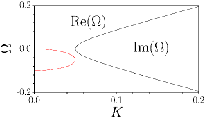
Figure 1: (Color online) The real and imaginary parts of $\Omega$ as functions of $K$ (see eq. (3)) are shown in the case $\gamma=\Gamma=0.05$ and $u_{0}=0$.

It is convenient to transform eq. (1) into a hydrodynamic form by means of the substitution

$$\psi=\sqrt{\rho}\,\exp\left(i\int^{x}u(x^{\prime},t)\upd x^{\prime}\right)e^{-i\mu t}$$ (5)

which yields

$$\rho_{t}+(\rho u)_{x}=2\Gamma\rho(\rho_{0}-\rho),$$ (6)

$$u_{t}+uu_{x}+\rho_{x}+\left(\frac{\rho_{x}^{2}}{8\rho^{2}}-\frac{\rho_{xx}}{4\rho}\right)_{x}=-V_{x}.$$ (7)

The last term in the left-hand side of (7) describes the dispersion effects; the right-hand side of (6) describes the gain and loss effects in the system; the other terms in eqs. (6),(7) have standard hydrodynamic meaning.

3 Hydraulic approximation

In what follows we assume that the size $l$ of the obstacle is much greater than the “healing length” (equal to unity in our non-dimensional variables). In our numerical simulations we will use an obstacle potential in the form

$$V(x)=V_{m}\exp(-x^{2}/l^{2}),\quad l\gg 1.$$ (8)

All numerical plots below are obtained for $l=5$. We are interested in stationary patterns with $\rho_{t}\equiv 0,\,u_{t}\equiv 0$ generated by the steady flow of the condensate past a localized obstacle ($V(x)\to 0$ as $|x|\to\infty$), i.e. $\rho$ and $u$ must satisfy the boundary conditions

$$\rho\to\rho_{0},\quad u\to u_{0}\quad\text{as}\quad|x|\to\infty.$$ (9)

Then eq. (6) can be reduced to

$$(\rho u)_{x}=2\Gamma\rho(\rho_{0}-\rho)$$ (10)

and the stationary eq. (7) can be integrated once to give

$$\tfrac{1}{2}{u^{2}}+\rho+\frac{\rho_{x}^{2}}{8\rho^{2}}-\frac{\rho_{xx}}{4\rho}+V(x)=\tfrac{1}{2}{u_{0}^{2}}+\rho_{0}$$ (11)

For $l\gg 1$ it is natural to assume that the wave pattern has the characteristic length about $l$ and, hence, the dispersive terms in (11) having higher order derivatives are negligibly small compared with other terms; then we get

$$\tfrac{1}{2}{u^{2}}+\rho+V(x)=\tfrac{1}{2}{u_{0}^{2}}+\rho_{0}.$$ (12)

Integration of eq. (10) over space shows that stationary patterns satisfy the condition (see also [14])

$$\int_{-\infty}^{\infty}\rho(\rho_{0}-\rho)\upd x=0.$$ (13)

Excluding $u$ from Eqs. (12) and (10) we get the equation

$$\left(\rho\sqrt{u_{0}^{2}+2(\rho_{0}-\rho-V(x))}\right)_{x}=2\Gamma\rho(\rho_{0}-\rho)$$ (14)

which determines the dependence of $\rho$ on $x$ for a given potential $V(x)$ provided the solution satisfies the condition (9). This equation represents the so-called hydraulic approximation for our system. (It generalizes the well-known Thomas-Fermi approximation to non-zero flow velocity.)

At the tails of the wave pattern ($|x|\to\infty$) we can neglect the potential $V(x)$ and linearize eq. (14) with respect to small deviations $\rho-\rho_{0}$ from the steady state. This gives the asymptotic behavior

$$|\rho-\rho_{0}|\propto\exp\left(\frac{2\Gamma\rho_{0}u_{0}}{\rho_{0}-u_{0}^{2}}x\right)$$ (15)

which shows that such tails extending beyond the range of the potential can exist only under the condition

$$\frac{|\rho_{0}-u_{0}^{2}|}{\Gamma\rho_{0}u_{0}}\gg l.$$ (16)

This means that the sound velocity $c_{s}=\sqrt{\rho_{0}}$ separates two different regimes—subsonic ($u_{0}<c_{s}$) and supersonic ($u_{0}>c_{s}$)—with drastically different properties. We shall discuss them separately.

4 Subsonic flow

The hydraulic approximation describes the profiles of the disturbance well enough practically in the entire subsonic regime $u_{0}<\sqrt{\rho_{0}}$ if the velocity is not too close to the sound velocity. In fig. 2 we compare the direct numerical solution of eq. (1) with its hydraulic approximation obtained by the numerical solution of eq. (14); quite good agreement is observed (notice that in all simulations we use $\gamma=\Gamma=0.05$ that gives sound velocity $c_{s}=1$). Naturally, the asymptotic behavior (15) is also confirmed in the upstream flow $x<0$. However, there is no linearized solution decaying to zero at $x\to+\infty$, hence the transition to the asymptotic steady flow in the downstream region $x>0$ has to occur within the range of the potential $V(x)$, and this conclusion is confirmed by direct numerical solution. Indeed, as one observes in fig. 2, the stationary disturbance has a smooth shape with a very long monotonically decaying left tail. This tail is attached to the density dip located almost completely within the potential region. The amplitude of the disturbance (i.e. the difference between maximal and minimal density in the condensate) in the subsonic regime monotonically increases with growth of the potential strength. It is convenient to introduce the “number of particles”

$$N=\int_{-\infty}^{\infty}[\rho^{1/2}(x)-a]^{2}\upd x$$ (17)

disturbed by the flow. This variable monotonically increases with the strength of potential [fig. 3(a)]. Interestingly, there exists a critical strength of potential $V_{m}^{cr}$ above which one cannot find stationary profiles. When $V_{m}\to V_{m}^{cr}$ the tangent to $N(V_{m})$ becomes vertical. For this strength of potential the amplitude of disturbance is maximal. Note that the critical potential strength $V_{m}^{cr}$ diverges when the incident velocity of the condensate $u_{0}\to 0$ and it monotonically decreases when $u_{0}$ increases [fig. 3(b)]. We were able to obtain the critical potential strength only for $0<u_{0}<0.8c_{s}$. For higher velocities $[0.8c_{s}<u_{0}<c_{s}]$ the condensate starts developing small oscillations on its right tail. Solutions characterized by different number of oscillations on their right tail may form continuous families that may be obtained even for potentials with $V_{m}>1$.

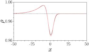
Figure 2: (Color online) Comparison of density profile at $u_{0}=0.6$, $V_{m}=0.1$, and $\gamma=\Gamma=0.05$ obtained numerically from eq. (1) (black curve) and in the framework of the hydraulic approximation (red curve). The dashed line shows plane wave solution (2) in absense of potential.

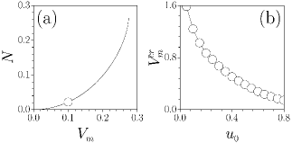
Figure 3: (a) Number of particles (17) versus potential strength for subsonic flow with $u_{0}=0.6$. The circle corresponds to the parameters used in fig. 2. (b) Critical strength of potential versus $u_{0}$. In all cases $\gamma=\Gamma=0.05$.

The condition (16) breaks down when the incident velocity $u_{0}$ is close to the critical value $\sqrt{\rho_{0}}$. In this case the potential $V(x)$ cannot be neglected in the hydraulic approximation (14. Even more, as $u_{0}$ approaches the critical value, the upstream density profile steepens and its slope can become so large that the dispersive terms in eq. (11) can no longer be neglected. As is known, the dispersive effects lead to generation of oscillations in the regions with fast change of the variables. Hence, for $u_{0}\gtrsim\sqrt{\rho_{0}}$ we should expect generation of dispersive shock waves and now we proceed to the discussion of the supersonic flow.

5 Supersonic flow

If $u_{0}>\sqrt{\rho_{0}}$ and the condition (16) is fulfilled, then the linearized solution (15) describes decaying disturbance in the downstream flow at $x\to+\infty$. Thus, contrarily to the subsonic case, the right tail for $x>0$ can extend far beyond the range of the potential.

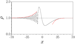
Figure 4: (Color online) The density distribution for shock wave at $u_{0}=1.4$, $V_{m}=0.8$, and $\gamma=\Gamma=0.05$. Red curves show analytical approximations of tails from eqs. (15) and (42). Dashed line shows plane wave solution in the absence of potential.

As mentioned above, the generation of an oscillatory dispersive shock wave is expected in the upstream flow. This is confirmed by numerical solution of (1) with the supersonic boundary conditions; see fig. 4. The dispersive shock waves can be represented as a modulated solution of the undisturbed ($\Gamma=\gamma=0,\,V(x)\equiv 0$) equation (1) or the system (6), (7) which can be written in the form (see, e.g., [16])

$$\begin{split}\rho(x,t)&=\nu_{1}+(\nu_{2}-\nu_{1})\mathrm{sn}^{2}(\sqrt{\nu_{3}-\nu_{1}}\,\theta,m)\\ &=\tfrac{1}{4}(\lambda_{1}-\lambda_{2}-\lambda_{3}+\lambda_{4})^{2}+(\lambda_{2}-\lambda_{1})(\lambda_{4}-\lambda_{3})\\ &\times\mathrm{sn}^{2}(\sqrt{(\lambda_{4}-\lambda_{2})(\lambda_{3}-\lambda_{1})}\,\theta,m),\end{split}$$ (18)

$$\begin{split}u(x,t)&=U-{q}/{\rho(x,t)},\\ q&=-\tfrac{1}{8}(\lambda_{1}-\lambda_{2}-\lambda_{3}+\lambda_{4})(\lambda_{1}-\lambda_{2}+\lambda_{3}-\lambda_{4})\\ &\times(\lambda_{1}+\lambda_{2}-\lambda_{3}-\lambda_{4}),\end{split}$$ (19)

where

$$\theta=x-Ut,\quad U=\tfrac{1}{2}(\lambda_{1}+\lambda_{2}+\lambda_{3}+\lambda_{4})$$ (20)

$\nu_{1},\nu_{2},\nu_{3}$ are related to the Riemann invariants $\lambda_{i},i=1,2,3,4,$ by the formulae

$$\begin{split}\nu_{1}&=\tfrac{1}{4}(\lambda_{1}-\lambda_{2}-\lambda_{3}+\lambda_{4})^{2},\\ \nu_{2}&=\tfrac{1}{4}(\lambda_{1}-\lambda_{2}+\lambda_{3}-\lambda_{4})^{2},\\ \nu_{3}&=\tfrac{1}{4}(\lambda_{1}+\lambda_{2}-\lambda_{3}-\lambda_{4})^{2},\end{split}$$ (21)

and

$$m=\frac{\nu_{2}-\nu_{1}}{\nu_{3}-\nu_{1}}=\frac{(\lambda_{2}-\lambda_{1})(\lambda_{4}-\lambda_{3})}{(\lambda_{3}-\lambda_{1})(\lambda_{4}-\lambda_{2})}.$$ (22)

In the modulated wave the Riemann invariants $\lambda_{i}$ become slow functions of $x$ and $t$ and their evolution is governed by the Whitham equations. They were derived for the case of eq. (1) with $\Gamma=0$ in [17] and their generalization to the nonzero $\Gamma$ is straightforward. Therefore we will write down here the final result without its derivation.

In our stationary case $\lambda_{i}$ do not depend on $t$ and the phase velocity $U$ equals to zero,

$$\lambda_{1}+\lambda_{2}+\lambda_{3}+\lambda_{4}=0.$$ (23)

Then the Whitham equations can be written in the form

$$\frac{\upd\lambda_{i}}{\upd x}=\frac{2}{L}\cdot\frac{I_{1}\lambda_{i}+I_{2}}{\prod_{m\neq i}(\lambda_{i}-\lambda_{m})},$$ (24)

where

$$\begin{split}I_{1}&=\Gamma\int_{\nu_{1}}^{\nu_{2}}\frac{\nu(\rho_{0}-\nu)}{\sqrt{\mathcal{R}(\nu)}}\upd\nu,\\ I_{2}&=\frac{\Gamma u_{0}\rho_{0}}{2}\int_{\nu_{1}}^{\nu_{2}}\frac{\rho_{0}-\nu}{\sqrt{\mathcal{R}(\nu)}}\upd\nu,\end{split}$$ (25)

$$\mathcal{R}=(\nu-\nu_{1})(\nu-\nu_{2})(\nu-\nu_{3})$$ (26)

and $L$ is the wavelength

$$L=\frac{2\mathrm{K}(m)}{\sqrt{(\lambda_{3}-\lambda_{1})(\lambda_{4}-\lambda_{2})}},$$ (27)

$\mathrm{K}(m)$ being the complete elliptic integral of the first kind.

Due to the special structure of Eqs. (24), the symmetric functions of $\lambda_{i}$,

$$\begin{split}s_{1}&=\sum_{i}\lambda_{i},\quad s_{2}=\sum_{i\neq j}\lambda_{i}\lambda_{j},\quad s_{3}=\sum_{i\neq j\neq k}\lambda_{i}\lambda_{j}\lambda_{k},\\ s_{4}&=\lambda_{1}\lambda_{2}\lambda_{3}\lambda_{4},\end{split}$$ (28)

obey very simple equations

$$\frac{\upd s_{1}}{\upd x}=0,\quad\frac{\upd s_{2}}{\upd x}=0,\quad\frac{\upd s_{3}}{\upd x}=\frac{2I_{1}}{L},\quad\frac{\upd s_{4}}{\upd x}=-\frac{2I_{2}}{L}.$$ (29)

The condensate density $\rho$ oscillates in the interval $\nu_{1}\leq\rho\leq\nu_{2}$, i.e. $\nu_{1}$ and $\nu_{2}$ are the envelopes of the oscillations in the dispersive shock wave. Let us study their asymptotic behavior at $x\to-\infty$.

The asymptotic plane wave corresponds to $\nu_{2}=\nu_{1}$ (or $\lambda_{2}=\lambda_{1}$) so that the parameters of the incident condensate are expressed in terms of the Riemann invariants as

$$\rho_{0}=\tfrac{1}{4}(\lambda_{4}-\lambda_{3})^{2}$$ (30)

and

$$u_{0}=\tfrac{1}{2}(\lambda_{3}+\lambda_{4}-2\lambda_{1}).$$ (31)

From (23), (30) and (31) we find the asymptotic values of the Riemann invariants

$$\begin{split}\lambda_{1}&=\lambda_{2}=-\frac{u_{0}}{2},\\ \lambda_{3}&=\frac{u_{0}}{2}-\sqrt{\rho_{0}},\quad\lambda_{4}=\frac{u_{0}}{2}+\sqrt{\rho_{0}}.\end{split}$$ (32)

The periodic solution corresponds to the ordering $\lambda_{1}\leq\lambda_{2}\leq\lambda_{3}\leq\lambda_{4}$, so that from $\lambda_{3}\geq\lambda_{2}$ we find that $u_{0}\geq\sqrt{\rho_{0}}$, i.e. the incident flow must be supersonic for the generation of such a stationary shock wave. The wavelength (27) of small amplitude oscillations ($m=0$) reduces in the limit $x\to-\infty$ to

$$L=\frac{\pi}{\sqrt{u_{0}^{2}-\rho_{0}}}.$$ (33)

The asymptotic values of $\nu_{1},\nu_{2},\nu_{3}$ at $x\to-\infty$ are $\nu_{1}(-\infty)=\nu_{2}(-\infty)=\rho_{0}$, $\nu_{3}(-\infty)=u_{0}^{2}$. We introduce small deviations from these values,

$$\nu_{1}=\rho_{0}+\delta\nu_{1},\quad\nu_{2}=\rho_{0}+\delta\nu_{2},\quad\nu_{3}=u_{0}^{2}+\delta\nu_{3},$$ (34)

and linearize eqs. (29) with respect to $\delta\nu_{i}$ with account of the identities

$$\begin{split}&\nu_{1}+\nu_{2}+\nu_{3}=-2s_{2},\\ &\nu_{1}\nu_{2}+\nu_{1}\nu_{3}+\nu_{2}\nu_{3}=-s_{2}^{2}+4s_{4},\quad\nu_{1}\nu_{2}\nu_{3}=s_{3}^{2}.\end{split}$$ (35)

As a result we arrive at the equations

$$\frac{\upd(\delta\nu_{1}+\delta\nu_{2})}{\upd x}=-\frac{\upd\delta\nu_{3}}{\upd x}=\frac{2\Gamma\rho_{0}u_{0}}{u_{0}^{2}-\rho_{0}}(\delta\nu_{1}+\delta\nu_{2}).$$ (36)

Hence we get

$$\delta\nu_{1}+\delta\nu_{2},\delta\nu_{3}\propto\exp\left(\frac{2\Gamma\rho_{0}u_{0}}{u_{0}^{2}-\rho_{0}}x\right).$$ (37)

These equations suggest that the sum of deviations $\delta\nu_{1}+\delta\nu_{2}$ decays at $x\to-\infty$ faster than the deviations $\delta\nu_{1}$ and $\delta\nu_{2}$ separately. If we introduce small deviations of the Riemann invariants from their asymptotic values (32)

$$\begin{split}\lambda_{1}&=-\frac{u_{0}}{2}+\delta\lambda_{1},\quad\lambda_{2}=-\frac{u_{0}}{2}+\delta\lambda_{2}\\ \lambda_{3}&=\frac{u_{0}}{2}-\sqrt{\rho_{0}}+\delta\lambda_{3},\quad\lambda_{4}=\frac{u_{0}}{2}+\sqrt{\rho_{0}}+\delta\lambda_{4},\end{split}$$ (38)

then we find that the asymptotic behavior (37) corresponds to $|\delta\lambda_{3}|,|\delta\lambda_{4}|\ll|\delta\lambda_{1}|,|\delta\lambda_{2}|$ so that

$$\begin{split}&\nu_{1}\cong\tfrac{1}{4}(2\sqrt{n_{0}}+\delta\lambda_{1}-\delta\lambda_{2})^{2},\\ &\nu_{2}\cong\tfrac{1}{4}(2\sqrt{n_{0}}-\delta\lambda_{1}+\delta\lambda_{2})^{2},\\ &\nu_{3}\cong\tfrac{1}{4}(2u_{0}-\delta\lambda_{1}-\delta\lambda_{2})^{2},\end{split}$$ (39)

and in leading order approximation $\delta\nu_{1}+\delta\nu_{2}=0$ which means that (37) corresponds to higher order corrections.

Thus, in the main approximation we assume that $\nu_{3}\cong u_{0}^{2}$ and from (25) we obtain the following equations for $\delta\lambda_{1}$ and $\delta\lambda_{2}$:

$$\begin{split}\frac{\upd\delta\lambda_{1}}{\upd x}&=\frac{\Gamma\rho_{0}u_{0}}{2(u_{0}^{2}-\rho_{0})}(\delta\lambda_{1}-\delta\lambda_{2}),\\ \frac{\upd\delta\lambda_{2}}{\upd x}&=-\frac{\Gamma\rho_{0}u_{0}}{2(u_{0}^{2}-\rho_{0})}(\delta\lambda_{1}-\delta\lambda_{2}).\end{split}$$ (40)

From these equations we get

$$\delta\lambda_{1,2}\cong\pm C\exp\left(\frac{\Gamma\rho_{0}u_{0}}{u_{0}^{2}-\rho_{0}}x\right)$$ (41)

($C$ is the integration constant), and hence the envelopes of oscillations in the dispersive shock decay at leading order approximation as

$$\delta\nu_{1},\delta\nu_{2}\propto\exp\left(\frac{\Gamma\rho_{0}u_{0}}{u_{0}^{2}-\rho_{0}}x\right).$$ (42)

This is slower than the dependence in (37) as it should be.

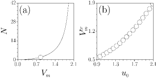
Figure 5: (a) Number of particles versus potential strength for supersonic flow with $u_{0}=1.4$. The circle corresponds to solution in fig. 4. (b) Critical strength of potential versus $u_{0}$. In all cases $\gamma=\Gamma=0.05$.

These analytical predictions were confirmed by the direct solution of eq. (1). As one can see from fig. 4, a typical shock wave solution may extend far beyond the repulsive potential, both in the positive and negative $x$ directions. Note the excellent agreement at $x\to\pm\infty$ between the numerical density and its analytical fit that uses the expressions (15) and (42). The wavelength of small amplitude oscillations estimated numerically for the parameters of the flow shown in fig. 4 is equal to $L_{num}\cong 3.16$ and the analytical formula (33) gives $L_{theor}\cong 3.21$, with an accuracy better than 2%. It should be stressed that the solution in fig. 4 is fully stationary (that is, it does not change in time), in contrast to previously reported one-dimensional shock waves in conservative systems. The oscillating left tail of the dispersive shock wave in the supersonic regime becomes more pronounced with increase of potential strength $V_{m}$ and incident velocity $u_{0}$. Just as for the subsonic flow the increase of $V_{m}$ is accompanied by an increase of the amplitude of the shock wave. However, in the supersonic regime the amplitude of shock wave may be comparable with the amplitude of the unperturbed plane wave and the density may decrease almost to zero in the downstream region, especially for strong potentials. The number of particles in the shock wave increases with $V_{m}$ [fig. 5(a)] and the character of this dependence also points to the existence of a critical defect strength beyond which shock waves do not exist.

A linear stability analysis performed for stationary solutions shows that wave patterns are stable for any strength of potential $V_{m}$ up to the critical one as long as the incident velocity is small enough, $u_{0}<0.9c_{s}$. When $u_{0}>0.9c_{s}$, stationary solutions become unstable if the strength of potential exceeds certain limiting value $V_{m}^{cr}$ (the instability of the dispersive shock waves at $V_{m}>V_{m}^{cr}$ is accompanied by the development and emission of small-scale disturbances on the right tail of the shock wave). Still, even shock waves with very long oscillating tails, like the one shown in fig.4, may be stable. The critical value of potential increases monotonically with $u_{0}$ as it is shown in fig. 5(b).

6 Conclusion

It is instructive to compare our results with those obtained in the case of the flow of a conservative fluid past an obstacle. As was shown in [12], in the conservative case one can distinguish three characteristic ranges of flow velocity—subcritical ($u_{0}<u_{-}$), transcritical ($u_{-}<u_{0}<u_{+}$), and supercritical ($u_{0}>u_{+}$) where the critical values of the velocity are located at opposite sides of the value of the sound velocity ($u_{-}<c_{s}<u_{+}$). If the flow velocity is subcritical or supercritical, then the disturbance is stationary and has the dimension of the obstacle’s size with definite sign of the difference $\rho-\rho_{0}$; it has a form of a dip in subcritical region and of a hump in supercritical region. In the present case of non-conservative dynamics the disturbance must have “dips” and “humps” to be compensated in the integral (13). Examples of such disturbances shown in figs. 2 and 4 demonstrate this property.

In the conservative situation the transcritical regime corresponds to non-stationary generation of upstream and/or downstream dispersive shock waves. In the non-conservative situation this regime actually disappears and instead a supersonic flow generates a stationary dispersive shock wave upstream the obstacle. There are no downstream dispersive shock waves; instead they are replaced by smooth profiles decaying asymptotically to the stationary plane wave.

The above properties of the wave patterns generated by the flow of polariton condensate past an obstacle are derived for the model (1). We believe, however, that these properties remain qualitatively the same for other models having stationary plane wave states formed due to balance of pumping and dissipation effects. In particular, this theory can find applications to a so-called “superfluid motion of light” [18, 19, 20].

- [1] \NameKeeling J., Marchetti F. M., Szymańska M. H. Littlewood P.B. \REVIEWSemicond. Sci. Technol.222007R1.
- [2] \NameAmo A., Sunvitto D. Viña L. \REVIEWSemicond. Sci. Technol.252010043001.
- [3] \NameKasprzak J., Richard M., Kundermann S., Baas A., Jeambrun P., Keeling J. M. J., Marchetti F. M., Szymańska M. H., André R., Staehli J. L., Savona V., Littlewood P. B., Deveaud B. Dang Le Si \REVIEWNature4432006409.
- [4] \NameLai C. W., Kim N. Y., Utsunomiya S., Roumpos G., Deng H., Fraser M. D., Byrnes T., Recher P., Kumada N., Fujisawa T. Yamamoto Y. \REVIEWNature4502007529.
- [5] \NameAmo A., Pigeon S., Sunvitto D., Sala V. G., Hivet R., Carusotto I., Pisanello F., Lemenager G., Houdré R., Giacobino E., Ciuti C., Bramati A. \REVIEWScience33220111167.
- [6] \NameGrosso G., Nardin G., Morier-Genoud F., Léger Y., Deveaud-Plédran B. \REVIEWarXiv: 1109.68592011.
- [7] \NameWertz E., Ferrier L., Solnyshkov D. D., Johne R., Sanvitto D., Lemaître A., Sagnes I., Grousson R., Kavokin A. V., Senellart P., Malpeuch G. Bloch J. \REVIEWNat. Phys.62010860.
- [8] \NameHakim V. \REVIEWPhys. Rev. E5519972835.
- [9] \NamePavloff N. \REVIEWPhys. Rev. A662002013610.
- [10] \NameRadouani A. \REVIEWPhys. Rev. A702004013602.
- [11] \NameEngels P. Atherton C. \REVIEWPhys. Rev. Lett.992007160405.
- [12] \NameLeszczyszyn A. M., El G. A., Gladush Yu. G. Kamchatnov A. M. \REVIEWPhys. Rev. A792009063608.
- [13] \NameKavokin A. V. Malpeuch G. \BookCavity Polaritons \PublElsevier \Year2003.
- [14] \NameKeeling J. Berloff N. G. \REVIEWPhys. Rev. Lett.1002008250401.
- [15] \NameWouters M. Carusotto I. \REVIEWPhys. Rev. Lett.992007140402.
- [16] \NameKamchatnov A. M. \BookNonlinear Periodic Waves and Their Modulations \PublWorld Scientific, Singapore \Year2000.
- [17] \NameKamchatnov A. M. \REVIEWPhysica D1882004247.
- [18] \NamePomeau Y. Rica S. \REVIEWC. R. Acad. Sci. Paris,31719931287.
- [19] \NameBolda E. L., Chiao R. Y., Zurek W. H. \REVIEWPhys. Rev. Lett.862001416.
- [20] \NameLeboeuf P. Moulieras S. \REVIEWPhys. Rev. Lett.1052010163904.