Evaluation of the screened vacuum-polarization corrections to the hyperfine splitting of Li-like bismuth

Abstract

The rigorous calculation of the vacuum-polarization screening corrections to the hyperfine splitting in Li-like bismuth is presented. The two-electron diagrams with electric and magnetic vacuum-polarization loops are evaluated to all orders in $\alpha Z$, including the Wichmann-Kroll contributions. This improves the accuracy of the theoretical prediction for the specific difference of the hyperfine splitting values of H- and Li-like bismuth.

I Introduction

High-precision measurements of the ground-state hyperfine splitting (HFS) were performed for various heavy H-like ions, including ²⁰⁹Bi, ¹⁶⁵Ho, ¹⁸⁵Re, ²⁰⁷Pb, ²⁰³Tl and ²⁰⁵Tl kl-prl-73 ; cr-prl-77 ; cr-pra-57 ; se-prl-81 ; be-pra-64 . Progress in experiments motivated intensive theoretical calculations of the hyperfine splitting in highly charged heavy ions sc-pra-50 ; sh-jpb-27 ; sh-pra-52 ; persson:96:prl ; bl-pra-55 ; sh-pra-56 ; su-pra-58 ; shabaev:98:hi ; boucard:00:epjd ; shabaev:00:hi ; sa-pra-63 ; sh-prl-86 ; ar-pra-63 ; ye-pra-64 aiming to test quantum electrodynamics (QED) in strong electromagnetic fields. It was found that in heavy ions the QED effects are obscured by the uncertainty of the nuclear magnetization distribution correction (Bohr-Weisskopf effect). However, simultaneous study of H- and Li-like ions of the same isotope can help to overcome this problem, since the uncertainty of the Bohr-Weisskopf effect is significantly reduced in the specific difference of the corresponding HFS values sh-prl-86 . High-precision measurements of the hyperfine splitting of H- and Li-like bismuth are feasible at the experimental storage ring (ESR) and the HITRAP facility in GSI an-hi-196 ; no-hi-199 . Recently, after 13 years of attempts, the HFS of the ground state Li-like Bi has been directly observed in GSI no-hi-pc . These measurements together with accurate theoretical calculations will provide the possibility for the stringent tests of QED in strong fields.

The recent improvements of the theoretical accuracy for the specific difference of the HFS values are related to the calculations of the screened QED corrections vo-prl-103 ; gl-pra-81 and the two-photon exchange corrections vo-prl-2011 to the HFS of the Li-like ions. Now the uncertainty of the specific HFS difference is mainly determined by the Wichmann-Kroll part of the screened QED corrections. In Refs. sa-pra-63 ; sapirstein:08:pra ; or-oas-102 ; ko-pra-76 ; or-pla-372 ; vo-pra-78 the screened QED corrections were evaluated by introducing an effective local screening potential in the zeroth-order (Dirac) equation. However, the screening potential approximation does not provide reliable estimation of the uncertainty. Recently, the two-electron self-energy diagrams and a dominant part of the two-electron vacuum-polarization diagrams, which represent the leading contribution to this effect, have been evaluated within the systematic QED approach vo-prl-103 ; gl-pra-81 . The present paper is devoted to the rigorous evaluation of the two-electron vacuum-polarization diagrams, which have been treated approximately in Refs. vo-prl-103 ; gl-pra-81 . In particular, the electric-loop and magnetic-loop diagrams are evaluated to all orders in $\alpha Z$, including the Wichmann-Kroll contributions. The Wichmann-Kroll terms of the remaining internal-loop contributions are estimated. The numerical results are presented for the hyperfine structure of Li-like bismuth ${}^{209}\textrm{Bi}^{80+}$.

The relativistic units ($\hbar=1$, $c=1$, $m=1$) and the Heaviside charge unit [${\alpha=e^{2}/(4\pi),e<0}$] are used throughout the paper.

II Basic formulas

The interaction of atomic electrons with the nuclear magnetic moment is described by the Fermi-Breit operator,

$$H_{\mu}=\frac{|e|}{4\pi}\bm{\mu}\cdot{\bf T}\,,$$ (1)

where $\bm{\mu}$ is the operator of the nuclear magnetic moment. The electronic operator ${\bf T}$ is given by

$${\bf T}=\sum_{i}\frac{[{\bf n}_{i}\times{\bm{\alpha}}_{i}]}{r_{i}^{2}}F(r_{i})\,,$$ (2)

where the summation runs over the atomic electrons, ${\bm{\alpha}}$ is the Dirac-matrix vector, ${\bf n}_{i}={\bf r}_{i}/r_{i}$, and $F(r)$ is the nuclear magnetization distribution factor (see, e.g., Refs. sh-pra-56 ; vo-pra-78 ). Here we employ the homogeneous sphere model,

$$F(r)=\begin{cases}(r/R_{0})^{3},&\mbox{if }r\leq R_{0}\,,\\ 1,&\mbox{if }r>R_{0}\,,\end{cases}$$ (3)

where $R_{0}$ is the radius of the sphere, related to the root-mean-square charge radius ${\langle r^{2}\rangle}^{1/2}$ of the nucleus as $R_{0}=\sqrt{5/3}{\langle r^{2}\rangle}^{1/2}$. The ground-state hyperfine splitting of a highly charged Li-like ion in the non-recoil limit can be written as

$$\Delta E_{\text{hfs}}^{(a)}=\frac{\alpha(\alpha Z)^{3}}{12}\frac{g_{I}}{m_{p}}(2I+1) \left[A(\alpha Z)(1-\delta)(1-\varepsilon)+\frac{1}{Z}B(\alpha Z)+\frac{1}{Z^{2}}C(\alpha Z)\right.$$ (4)

$$\left.+\frac{1}{Z^{3}}D(Z,\alpha Z)+x_{\text{QED}}+x_{\text{SQED}}\right]\,.$$

Here $g_{I}=\mu/(\mu_{N}I)$ is the $g$ factor of the nucleus with magnetic moment $\mu$ and spin $I$, $\mu_{N}$ is the nuclear magneton, and $m_{p}$ denotes the proton mass. $A(\alpha Z)$ is the one-electron relativistic factor, $\delta$ and $\varepsilon$ are the corrections due to the finite distribution of the charge and the magnetic moment over the nucleus, respectively, which can be found either analytically sh-jpb-27 ; vo-epjd-23 or numerically. The interelectronic-interaction correction of first order in $1/Z$ is represented by the function $B(\alpha Z)$. The function $C(\alpha Z)$ incorporates the interelectronic-interaction corrections in the second order in $1/Z$, $D(Z,\alpha Z)$ corresponds to the third- and higher-order corrections in $1/Z$. $x_{\text{QED}}$ and $x_{\text{SQED}}$ correspond to the one-electron and many-electron (screened) QED corrections, respectively.

To first order in $\alpha$ and $1/Z$, the screened QED correction $x_{\text{SQED}}$ to the hyperfine splitting is given by the sum of the self-energy (SE) and vacuum-polarization (VP) parts

$$x_{\text{SQED}}=x_{\text{SQED}}^{\text{SE}}+x_{\text{SQED}}^{\text{VP}}.$$ (5)

In the present paper the vacuum-polarization part $x_{\text{SQED}}^{\text{VP}}$ is considered. The corresponding diagrams are depicted in Fig. 1.

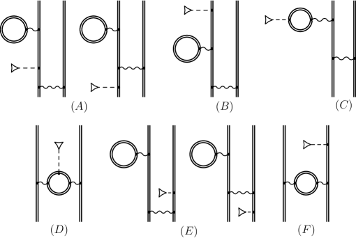
Figure 1: Diagrams, contributing to the screened VP correction to the hyperfine splitting. The wavy line indicates the photon propagator and the double line indicates the electron propagator in the Coulomb field. The dashed line terminated by the triangle denotes the interaction with the nuclear magnetic field.

The total contribution of these diagrams is conveniently divided into reducible and irreducible parts. The irreducible parts of each diagram A–F are denoted by the same letter: $x_{\text{SQED}}^{\text{VP(A-F)}}$. The reducible contributions are to be considered together with the non-diagram terms (see Ref. gl-pra-81 for details). They are divided into three parts, G, H, and I, according to the type of the vacuum-polarization loop: G is associated with the electric-loop diagrams A, B, and E; H corresponds to the magnetic-loop diagram C; and I — to the internal-loop diagram F.

The total correction due to the two-electron vacuum-polarization is given by the sum

$$x_{\text{SQED}}^{\text{VP}} = x_{\text{SQED}}^{\text{VP(A)}}+x_{\text{SQED}}^{\text{VP(B)}}+x_{\text{SQED}}^{\text{VP(C)}}+x_{\text{SQED}}^{\text{VP(D)}}+x_{\text{SQED}}^{\text{VP(E)}}+x_{\text{SQED}}^{\text{VP(F)}}$$ (6)

$$+x_{\text{SQED}}^{\text{VP(G)}}+x_{\text{SQED}}^{\text{VP(H)}}+x_{\text{SQED}}^{\text{VP(I)}}\,.$$

II.1 Electric-loop diagrams

The terms A, B, E, and G in Eq. (6) correspond to the so-called electric-loop (el) diagrams A, B and E. The contributions of these terms are given by the following expressions vo-prl-103 ; gl-pra-81

$$x_{\text{SQED}}^{\text{VP(A)}}=2\,G_{a}\sum_{b}\sum_{PQ}(-1)^{P+Q} \left[{\sum_{n_{1},n_{2}}}^{\prime}\langle Pa|U_{\text{VP}}^{\text{el}}|n_{1}\rangle\frac{\langle n_{1}|T_{0}|n_{2}\rangle\langle n_{2}Pb|I(\Delta)|QaQb\rangle}{(\varepsilon_{Pa}-\varepsilon_{n_{1}})(\varepsilon_{Pa}-\varepsilon_{n_{2}})}\right.$$ (7)

$$\left.+{\sum_{n_{1},n_{2}}}^{\prime}\langle Pa|U_{\text{VP}}^{\text{el}}|n_{1}\rangle\frac{\langle n_{1}Pb|I(\Delta)|n_{2}Qb\rangle\langle n_{2}|T_{0}|Qa\rangle}{(\varepsilon_{Pa}-\varepsilon_{n_{1}})(\varepsilon_{Qa}-\varepsilon_{n_{2}})}\right]\,,$$

$$x_{\text{SQED}}^{\text{VP(B)}}=2\,G_{a}\sum_{b}\sum_{PQ}(-1)^{P+Q}{\sum_{n_{1},n_{2}}}^{\prime}\frac{\langle Pa|T_{0}|n_{1}\rangle}{\varepsilon_{Pa}-\varepsilon_{n_{1}}}\langle n_{1}|U_{\text{VP}}^{\text{el}}|n_{2}\rangle\frac{\langle n_{2}Pb|I(\Delta)|QaQb\rangle}{\varepsilon_{Pa}-\varepsilon_{n_{2}}}\,,$$ (8)

$$x_{\text{SQED}}^{\text{VP(E)}}=2\,G_{a}\sum_{b}\sum_{PQ}(-1)^{P+Q} \left[{\sum_{n_{1},n_{2}}}^{\prime}\langle Pa|U_{\text{VP}}^{\text{el}}|n_{1}\rangle\frac{\langle Pb|T_{0}|n_{2}\rangle\langle n_{1}n2|I(\Delta)|QaQb\rangle}{(\varepsilon_{Pa}-\varepsilon_{n_{1}})(\varepsilon_{Pb}-\varepsilon_{n_{2}})}\right.$$ (9)

$$\left.+{\sum_{n_{1},n_{2}}}^{\prime}\langle Pa|U_{\text{VP}}^{\text{el}}|n_{1}\rangle\frac{\langle n_{1}Pb|I(\Delta)|Qan_{2}\rangle\langle n_{2}|T_{0}|Qb\rangle}{(\varepsilon_{Pa}-\varepsilon_{n_{1}})(\varepsilon_{Qb}-\varepsilon_{n_{2}})}\right]\,,$$

$$x_{\text{SQED}}^{\text{VP(G)}} = -2\,G_{a}\sum_{b}\sum_{PQ}(-1)^{P+Q}{\sum_{n_{1}}}^{\prime}\frac{1}{(\varepsilon_{Pa}-\varepsilon_{n_{1}})^{2}}$$ (10)

$$\left\{\langle Pa|U_{\text{VP}}^{\text{el}}|n_{1}\rangle\langle n_{1}|T_{0}|Pa\rangle\langle PaPb|I(\Delta)|QaQb\rangle\right.$$

$$+\langle Pa|U_{\text{VP}}^{\text{el}}|Pa\rangle\langle Pa|T_{0}|n_{1}\rangle\langle n_{1}Pb|I(\Delta)|QaQb\rangle$$

$$\left.+\langle Pa|T_{0}|Pa\rangle\langle Pa|U_{\text{VP}}^{\text{el}}|n_{1}\rangle\langle n_{1}Pb|I(\Delta)|QaQb\rangle\right\}$$

$$+2\,G_{a}\sum_{b}\sum_{PQ}(-1)^{P+Q}\left\{{\sum_{n_{1}}}^{\prime}\frac{1}{\varepsilon_{Pa}-\varepsilon_{n_{1}}}\right.$$

$$\times\left[\langle Pa|U_{\text{VP}}^{\text{el}}|n_{1}\rangle\langle n_{1}|T_{0}|Pa\rangle\langle PaPb|I^{\prime}(\Delta)|QaQb\rangle\right.$$

$$\left.+\langle Pa|U_{\text{VP}}^{\text{el}}|n_{1}\rangle\langle n_{1}Pb|I^{\prime}(\Delta)|QaQb\rangle\left(\langle Qb|T_{0}|Qb\rangle-\langle Pb|T_{0}|Pb\rangle\right)\right]$$

$$+\langle Pa|U_{\text{VP}}^{\text{el}}|Pa\rangle\left[{\sum_{n_{1}}}^{\prime}\frac{\langle PaPb|I^{\prime}(\Delta)|n_{1}Qb\rangle\langle n_{1}|T_{0}|Qa\rangle}{\varepsilon_{Qa}-\varepsilon_{n_{1}}}\right.$$

$$\left.\left.+{\sum_{n_{1}}}^{\prime}\frac{\langle PaPb|I^{\prime}(\Delta)|Qan_{1}\rangle\langle n_{1}|T_{0}|Qb\rangle}{\varepsilon_{Qb}-\varepsilon_{n_{1}}}\right]\right\}$$

$$+G_{a}\sum_{b}\sum_{PQ}(-1)^{P+Q}\langle Pa|U_{\text{VP}}^{\text{el}}|Pa\rangle\langle PaPb|I^{\prime\prime}(\Delta)|QaQb\rangle$$

$$\times\left(\langle Qb|T_{0}|Qb\rangle-\langle Pb|T_{0}|Pb\rangle\right)\,.$$

Here and below (Eqs. (16), (17), (30), (31)) $P$ and $Q$ are the permutation operators, interchanging $a$ and $b$, $\Delta\equiv\varepsilon_{Qb}-\varepsilon_{Qa}$. The summation over $b$ runs over two core electron states with different projections of the angular momentum. The prime at the summation sign ${\sum}^{\prime}$ indicates that the energy of the intermediate state differs from the energy of the initial state, so that the corresponding denominator is non-zero. The interelectronic-interaction operator $I(\Delta)$ and its derivatives are defined as in Ref. sh-pr-356 . The factor $G_{a}$ is defined by the quantum numbers of the valence state,

$$G_{a}=\frac{n^{3}(2l+1)j(j+1)}{2(\alpha Z)^{3}m_{j}}=\frac{3}{(\alpha Z)^{3}m_{j}}\,,$$ (11)

where $m_{j}$ is the projection of the angular momentum $j$.

Equations (7)–(10) involve the matrix elements of the standard electric-field-induced vacuum-polarization potential $U_{\text{VP}}^{\text{el}}$. The unrenormalized expression for $U_{\text{VP}}^{\text{el}}$ is given by

$$U_{\text{VP}}^{\text{el}}({\bf r})=\frac{\alpha}{2\pi i}\int d^{3}{\bf r}^{\prime}\,\frac{1}{|{\bf r}-{\bf r}^{\prime}|}\int_{-\infty}^{\infty}d\omega\,\text{Tr}[G(\omega,{\bf r}^{\prime},{\bf r}^{\prime})]\,,$$ (12)

where $G(\omega,{\bf r},{\bf r}^{\prime})$ is the Dirac-Coulomb Green function

$$G(\omega,{\bf r},{\bf r}^{\prime})=\sum_{n}\frac{\psi_{n}({\bf r})\psi_{n}^{\dagger}({\bf r}^{\prime})}{\omega-\varepsilon_{n}(1-i0)}\,.$$ (13)

The decomposition of the vacuum-polarization loop into the Uehling (Ue) and the Wichmann-Kroll (WK) terms is depicted in Fig. 2. In this expansion only the lowest order term, the Uehling term, is divergent. The charge renormalization yields a finite well known renormalized expression

$$U_{\text{VP}}^{\text{el-Ue}}(r) = -\alpha Z\,\frac{2\alpha}{3\pi}\int_{0}^{\infty}d{r^{\prime}}\,4\pi{r^{\prime}}\,\rho({r^{\prime}})\int_{1}^{\infty}dt\,\left(1+\frac{1}{2t^{2}}\right)\frac{\sqrt{t^{2}-1}}{t^{2}}$$ (14)

$$\times\frac{1}{4rt}\left[\exp(-2|r-{r^{\prime}}|t)-\exp(-2(r+{r^{\prime}})t)\right]\,,$$

where the density of the nuclear charge distribution $\rho(r)$ is normalized to 1. The Wichmann-Kroll part (the term in brackets in the decomposition in Fig. 2) is calculated to all orders in $\alpha Z$ as the difference between the unrenormalized total and Uehling contributions. The resulting expression is free from divergencies, completely isolated in the Uehling term mo-pr-293 . It is known, that no spurious terms contribute, if the calculation is based on the the partial-wave expansion of the electron Green function and the summation is terminated after a finite number of terms gy-npa-244 ; ri-pra-12 ; so-pra-38 . Thus the WK contribution after Wick-rotation of the contour of $\omega$-integration in the complex plane can be written as ar-pra-60

$$U_{\text{VP}}^{\text{el-WK}}(r) = \frac{2\alpha}{\pi}\sum_{\kappa}|\kappa|\int_{0}^{\infty}d\omega\int_{0}^{\infty}d{r^{\prime}}\,{r^{\prime}}^{2}\int_{0}^{\infty}d{r^{\prime\prime}}\,{r^{\prime\prime}}^{2}\frac{1}{\text{max}(r,{r^{\prime}})}V({r^{\prime\prime}})$$ (15)

$$\times\sum_{i,k=1}^{2}\text{Re}\left\{F_{\kappa}^{ik}(i\omega,{r^{\prime}},{r^{\prime\prime}})[G_{\kappa}^{ik}(i\omega,{r^{\prime}},{r^{\prime\prime}})-F_{\kappa}^{ik}(i\omega,{r^{\prime}},{r^{\prime\prime}})]\right\}\,.$$

Here $G_{\kappa}^{ik}$ and $F_{\kappa}^{ik}$ are the radial components of the partial-wave contributions to the bound and free electron Green’s functions, respectively, and $V(r)$ is the electric potential of the extended nucleus.

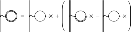
Figure 2: The decomposition of the $U_{\text{VP}}^{\text{el}}$ into the Uehling (Ue) and the Wichmann-Kroll (WK) terms.

II.2 Magnetic-loop diagrams

The magnetic-loop (ml) diagram C corresponds to the terms C and H in Eq. (6), given by vo-prl-103 ; gl-pra-81

$$x_{\text{SQED}}^{\text{VP(C)}}=2\,G_{a}\sum_{b}\sum_{PQ}(-1)^{P+Q}{\sum_{n_{1}}}^{\prime}\langle Pa|U_{\text{VP}}^{\text{ml}}|n_{1}\rangle\frac{\langle n_{1}Pb|I(\Delta)|QaQb\rangle}{\varepsilon_{Pa}-\varepsilon_{n_{1}}}\,,$$ (16)

$$x_{\text{SQED}}^{\text{VP(H)}}=\frac{1}{2}\,G_{a}\sum_{b}\sum_{PQ}(-1)^{P+Q}\langle PaPb|I^{\prime}(\Delta)|QaQb\rangle\left(\langle Qb|U_{\text{VP}}^{\text{ml}}|Qb\rangle-\langle Pb|U_{\text{VP}}^{\text{ml}}|Pb\rangle\right)\,.$$ (17)

Equations (16), (17) involve the matrix elements of the magnetic-field-induced vacuum-polarization potential $U_{\text{VP}}^{\text{ml}}$. Its unrenormalized expression reads

$$U_{\text{VP}}^{\text{ml}}({\bf r})=\frac{\alpha}{2\pi i}\int_{-\infty}^{\infty}d\omega\int d^{3}{\bf r}^{\prime}\int d^{3}{\bf r}^{\prime\prime}\frac{{\bm{\alpha}}}{|{\bf r}-{\bf r}^{\prime}|}\text{Tr}[{\bm{\alpha}}G(\omega,{\bf r}^{\prime},{\bf r}^{\prime\prime})T_{0}({\bf r}^{\prime\prime})G(\omega,{\bf r}^{\prime\prime},{\bf r}^{\prime})]\,.$$ (18)

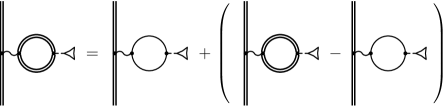
Figure 3: The decomposition of the $U_{\text{VP}}^{\text{ml}}$ into the Uehling and the Wichmann-Kroll terms.

The scalar product is implicit in Eq. (18). Similar to the electric-loop potential, the decomposition of the magnetic-loop potential into the first order term and the remainder (Fig. 3) leads to the isolation of the divergency in the leading Uehling term. It is given by the Eq. (18) with the bound-electron Green function replaced by the free-electron one. For the sphere model of the nuclear magnetization distribution ($F(r)$ given by Eq. (3)) the analytical expression for the renormalized magnetic-loop Uehling term reads vo-pra-78

$$U_{\text{VP}}^{\text{ml-Ue}}({\bf r})=\frac{\alpha}{\pi}\frac{[\textbf{n}\times{\bm{\alpha}}]_{0}}{r^{2}}\frac{3}{16R_{0}^{3}}\, \left[4rR_{0}[\beta_{1}(R_{0}+r)+\beta_{1}(|R_{0}-r|)]\right.$$ (19)

$$+2(R_{0}+r)\beta_{2}(R_{0}+r)-2|R_{0}-r|\beta_{2}(|R_{0}-r|)$$

$$\left.+\beta_{3}(R_{0}+r)-\beta_{3}(|R_{0}-r|)\right]\,,$$

where the function $\beta_{n}$ is defined by

$$\beta_{n}(r)=\frac{2}{3}\int_{1}^{\infty}dt\,\frac{\sqrt{t^{2}-1}}{t^{n+2}}\left(1+\frac{1}{2t^{2}}\right)\exp(-2tr)\,.$$ (20)

Similar to the case of electric-loop term, the magnetic-loop Wichmann-Kroll contribution is calculated by summing up the partial-wave differences between the unrenormalized total and Uehling contributions. The magnetic-loop diagram contributes also to the nuclear magnetic moment. The corresponding Uehling term is equal to zero, however the Wichmann-Kroll term is not. Therefore, in the calculations of the WK contribution one should account for the related contribution to the nuclear magnetic moment in the zeroth-order HFS value (see Refs. su-pra-58 ; ar-pra-63 ; mi-plb-233 ). This implies the replacement of the nuclear magnetic moment $\mu$ by the ‘bare’ value

$$\mu\rightarrow\mu_{\text{bare}}=\mu-\Delta\mu\,.$$ (21)

The nuclear magnetic moment correction $\Delta\mu$ due to the magnetic-loop WK part can be expressed as $\Delta\mu=\epsilon\mu$ with the dimensionless parameter $\epsilon$ given by

$$\epsilon=\frac{1}{2\pi i}\frac{\alpha}{2}\int d^{3}{\bf r}\int d^{3}{\bf r}^{\prime}\int_{-\infty}^{\infty}d\omega \left[\text{Tr}\left\{[{\bf r}\times{\bm{\alpha}}]_{0}G(\omega,{\bf r},{\bf r}^{\prime})T_{0}({\bf r}^{\prime})G(\omega,{\bf r}^{\prime},{\bf r})\right\}\right.$$ (22)

$$\left.-\text{Tr}\left\{[{\bf r}\times{\bm{\alpha}}]_{0}F(\omega,{\bf r},{\bf r}^{\prime})T_{0}({\bf r}^{\prime})F(\omega,{\bf r}^{\prime},{\bf r})\right\}\right]\,.$$

Finally, the corrected magnetic-loop WK contribution is obtained by subtraction of $\epsilon T_{0}$ from the WK part of Eq. (18). The corresponding expression reads

$$U_{\text{VP}}^{\text{ml-WK}}({\bf r}) = \frac{\alpha}{2\pi i}\int_{-\infty}^{\infty}d\omega\int d^{3}{\bf r}^{\prime}\int d^{3}{\bf r}^{\prime\prime}$$ (23)

$$\times\left(\frac{{\bm{\alpha}}}{|{\bf r}-{\bf r}^{\prime}|}\left[\text{Tr}\left\{{\bm{\alpha}}G(\omega,{\bf r}^{\prime},{\bf r}^{\prime\prime})T_{0}({\bf r}^{\prime\prime})G(\omega,{\bf r}^{\prime\prime},{\bf r}^{\prime})\right\}\right.\right.$$

$$\left.-\text{Tr}\left\{{\bm{\alpha}}F(\omega,{\bf r}^{\prime},{\bf r}^{\prime\prime})T_{0}({\bf r}^{\prime\prime})F(\omega,{\bf r}^{\prime\prime},{\bf r}^{\prime})\right\}\right]$$

$$-\frac{1}{2}\,T_{0}({\bf r})\left[\text{Tr}\left\{[{\bf r}^{\prime}\times{\bm{\alpha}}]_{0}G(\omega,{\bf r}^{\prime},{\bf r}^{\prime\prime})T_{0}({\bf r}^{\prime\prime})G(\omega,{\bf r}^{\prime\prime},{\bf r}^{\prime})\right\}\right.$$

$$\left.\left.-\text{Tr}\left\{[{\bf r}^{\prime}\times{\bm{\alpha}}]_{0}F(\omega,{\bf r}^{\prime},{\bf r}^{\prime\prime})T_{0}({\bf r}^{\prime\prime})F(\omega,{\bf r}^{\prime\prime},{\bf r}^{\prime})\right\}\right]\vphantom{\frac{{\bm{\alpha}}}{|{\bf x}-{\bf y}|}}\right)\,.$$

The angular-momentum conservation allows one to distinguish in this expression the following angular dependence

$$U_{\text{VP}}^{\text{ml-WK}}({\bf r})=[{\bf n}\times{\bm{\alpha}}]_{0}\,u_{\text{VP}}^{\text{ml-WK}}(r)\,.$$ (24)

The radial part $u_{\text{VP}}^{\text{ml-WK}}(r)$ can be presented in the form

$$u_{\text{VP}}^{\text{ml-WK}}(r)=\int_{0}^{\infty}d{r^{\prime}}{r^{\prime}}^{2}\left(\frac{r_{<}}{r_{>}^{2}}-\frac{{r^{\prime}}}{r^{2}}\,F(r)\right)\rho_{\text{ml}}({r^{\prime}})\,,$$ (25)

where the magnetic-loop WK charge density $\rho_{\text{ml}}({r^{\prime}})$ after rotating the contour of $\omega$-integration can be written as

$$\rho_{\text{ml}}({r^{\prime}})=\frac{\alpha}{6\pi}\int_{0}^{\infty}d{r^{\prime\prime}}F({r^{\prime\prime}})\int_{0}^{\infty}d\omega\sum_{\kappa_{1},\kappa_{2}}B^{2}(\kappa_{1},\kappa_{2})S_{\kappa_{1}\kappa_{2}}(\omega,{r^{\prime}},{r^{\prime\prime}})\,.$$ (26)

Here the Green-function trace $S_{\kappa_{1}\kappa_{2}}$ is given by

$$S_{\kappa_{1}\kappa_{2}}(\omega,{r^{\prime}},{r^{\prime\prime}})= \Big{\{}G^{11}_{\kappa_{1}}(i\omega,{r^{\prime}},{r^{\prime\prime}})\,G^{22}_{\kappa_{2}}(i\omega,{r^{\prime}},{r^{\prime\prime}})+G^{12}_{\kappa_{1}}(i\omega,{r^{\prime}},{r^{\prime\prime}})\,G^{21}_{\kappa_{2}}(i\omega,{r^{\prime}},{r^{\prime\prime}})$$ Re (27)

$$+G^{21}_{\kappa_{1}}(i\omega,{r^{\prime}},{r^{\prime\prime}})\,G^{12}_{\kappa_{2}}(i\omega,{r^{\prime}},{r^{\prime\prime}})+G^{22}_{\kappa_{1}}(i\omega,{r^{\prime}},{r^{\prime\prime}})\,G^{11}_{\kappa_{2}}(i\omega,{r^{\prime}},{r^{\prime\prime}})$$

$$-F^{11}_{\kappa_{1}}(i\omega,{r^{\prime}},{r^{\prime\prime}})\ F^{22}_{\kappa_{2}}(i\omega,{r^{\prime}},{r^{\prime\prime}})-F^{12}_{\kappa_{1}}(i\omega,{r^{\prime}},{r^{\prime\prime}})\ F^{21}_{\kappa_{2}}(i\omega,{r^{\prime}},{r^{\prime\prime}})$$

$$-F^{21}_{\kappa_{1}}(i\omega,{r^{\prime}},{r^{\prime\prime}})\ F^{12}_{\kappa_{2}}(i\omega,{r^{\prime}},{r^{\prime\prime}})-F^{22}_{\kappa_{1}}(i\omega,{r^{\prime}},{r^{\prime\prime}})\ F^{11}_{\kappa_{2}}(i\omega,{r^{\prime}},{r^{\prime\prime}})\Big{\}}\,,$$

and the angular factor $B(\kappa_{1},\kappa_{2})$ is defined by the following expression

$$B(\kappa_{1},\kappa_{2})=\frac{1+(-1)^{l_{1}+l_{2}}}{2}\sqrt{2(2j_{1}+1)(2j_{2}+1)}\,(-1)^{l_{1}}\left(\begin{array}[]{ccc}j_{1}&j_{2}&1\\ \frac{1}{2}&\frac{1}{2}&-1\\ \end{array}\right)\,.$$ (28)

The selection rule, following from this expression, forces $\kappa_{2}$ to be equal to either $\kappa_{1}$ or $-\kappa_{1}\pm 1$. Therefore the double $\kappa$-summation can be reduced to a single one, including diagonal and off-diagonal $\kappa$-terms,

$$\sum_{\kappa_{1},\kappa_{2}}B^{2}(\kappa_{1},\kappa_{2})S_{\kappa_{1}\kappa_{2}}=\sum_{\kappa}\left[\frac{2|\kappa|^{3}}{\kappa^{2}-1/4}S_{\kappa\kappa}+2\frac{|\kappa|(|\kappa|+1)}{|\kappa|+1/2}S_{\kappa\bar{\kappa}}\right]\,,$$ (29)

where $\bar{\kappa}=-\kappa-\text{sign}(\kappa)$.

II.3 Internal-loop diagrams

The internal-loop diagram F corresponds to the terms F and I in Eq. (6), given by vo-prl-103 ; gl-pra-81

$$x_{\text{SQED}}^{\text{VP(F)}}=2\,G_{a}\sum_{b}\sum_{PQ}(-1)^{P+Q}{\sum_{n_{1}}}^{\prime}\frac{\langle Pa|T_{0}|n_{1}\rangle}{\varepsilon_{Pa}-\varepsilon_{n_{1}}}\langle n_{1}Pb|I_{\text{VP}}(\Delta)|QaQb\rangle\,,$$ (30)

$$x_{\text{SQED}}^{\text{VP(I)}}=\frac{1}{2}\,G_{a}\sum_{b}\sum_{PQ}(-1)^{P+Q}\langle PaPb|I_{\text{VP}}^{\prime}(\Delta)|QaQb\rangle\left(\langle Qb|T_{0}|Qb\rangle-\langle Pb|T_{0}|Pb\rangle\right)\,.$$ (31)

Equations (30) and (31) involve the interelectronic-interaction operator, modified by the vacuum-polarization loop,

$$I_{\text{VP}}(\varepsilon,{\bf r}_{1},{\bf r}_{2}) = \frac{\alpha^{2}}{2\pi i}\int_{-\infty}^{\infty}d\omega\int d^{3}{\bf r}^{\prime}_{1}\int d^{3}{\bf r}^{\prime}_{2}\,\frac{\alpha_{1\mu}\exp(i|\varepsilon||{\bf r}_{1}-{\bf r}^{\prime}_{1}|)}{|{\bf r}_{1}-{\bf r}^{\prime}_{1}|}\,\frac{\alpha_{2\nu}\exp(i|\varepsilon||{\bf r}_{2}-{\bf r}^{\prime}_{2}|)}{|{\bf r}_{2}-{\bf r}^{\prime}_{2}|}$$ (32)

$$\times\text{Tr}\left[\alpha^{\mu}G(\omega-\varepsilon/2,{\bf r}^{\prime}_{1},{\bf r}^{\prime}_{2})\alpha^{\nu}G(\omega+\varepsilon/2,{\bf r}^{\prime}_{2},{\bf r}^{\prime}_{1})\right]\,,$$

where $\varepsilon$ is the energy of the transmitted photon, $\alpha^{\mu}=(1,{\bm{\alpha}})$ is the four-vector of the Dirac matrices, and the summation over $\mu$ and $\nu$ is implicit. The matrices $\alpha_{1\mu}$ and $\alpha_{2\nu}$ act on the spinor variables corresponding to ${\bf r}_{1}$ and ${\bf r}_{2}$, respectively. This operator is also divided into the leading divergent Uehling part and the remaining finite Wichmann-Kroll part (see Fig. 4). The renormalized expression for the Uehling term reads (see, e.g., ar-pra-60 )

$$I_{\text{VP}}^{\text{Ue}}(\varepsilon,{\bf r}_{1},{\bf r}_{2})=\frac{2\alpha^{2}}{3\pi}\,\frac{\alpha_{1\mu}\alpha^{\mu}_{2}}{|{\bf r}_{1}-{\bf r}_{2}|}\,\int_{1}^{\infty}dt\left(1+\frac{1}{2t^{2}}\right)\frac{\sqrt{t^{2}-1}}{t^{2}}\exp\left(-\sqrt{4t^{2}-\varepsilon^{2}}\,|{\bf r}_{1}-{\bf r}_{2}|\right)\,.$$ (33)

The corresponding contribution is taken into account rigorously. The direct part of the Wichmann-Kroll contribution with the hyperfine interaction vertex on the $2s$-electron line has been calculated by introducing the screening potential of the $(1s)^{2}$ closed shell electrons into the electric loop. We take the difference between the contributions with the Green function inside the loop calculated with and without the screening potential. The calculation of the direct part of the diagram D, which involves the internal loop modified by the hyperfine interaction vertex, has been performed in a similar way. It is evaluated by including the potential of the closed shell into the Green functions of the internal loop, that leads to a diagram of the magnetic-loop type. The evaluation of the remaining exchange diagrams is currently underway.

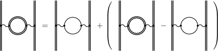
Figure 4: The decomposition of the internal electric-loop $I_{\text{VP}}$ into the Uehling and the Wichmann-Kroll terms.

III Results and discussion

The contribution of the two-electron vacuum-polarization diagrams to the hyperfine splitting of Li-like ion is calculated in coordinate space according to the formulas presented above. The electric-loop terms (A, B, E, G) and the magnetic-loop terms (C and H) are taken into account completely, including the Uehling and the Wichmann-Kroll parts. The internal-loop diagram F and the corresponding reducible term I are calculated rigorously in the Uehling approximation. The related WK contributions are evaluated for the direct parts with the hyperfine interaction vertex on the $2s$-electron. The remaining terms are estimated employing the assumption that the ratio of the WK part to the corresponding Uehling part is the same. The uncertainty is ascribed as high as $200\%$ of the value obtained in this way. The contribution of the direct part of the diagram D is evaluated as described in the previous section. We ascribe a $200\%$ uncertainty to the D contribution as a conservative estimation of the uncalculated exchange term. The numerical evaluation of the one-electron wave functions for the initial ($a$) and intermediate ($n_{1,2}$) states is performed using the dual kinetic balance (DKB) approach sh-prl-04 with the basis set constructed from the B-splines sapirstein:96:jpb . The Fermi model for the nuclear charge distribution is employed in these calculations. The Uehling parts of the vacuum-polarization potentials are calculated according to the expressions (14), (19), and (33). The Wichmann-Kroll parts involve the free- and bound-electron Green functions for the Dirac equation. The spherical shell model (possessing analytical solution for the bare nucleus case) and Fermi model of the nuclear charge distribution were employed in calculations of the Green function. The nuclear magnetization distribution effect is taken into account within the homogeneous sphere model. The partial-wave expansion is terminated at $|\kappa|=5$ in case of the electric-loop Wichmann-Kroll parts and at $|\kappa|=10$ in case of the magnetic-loop Wichmann-Kroll parts. The remainders of the k-summations are estimated using the least-square inverse-polynomial fitting. The numerical calculation procedure has been performed in different gauges, the gauge invariance should hold for the complete set of the two-electron vacuum-polarization diagrams. The total values obtained in the Feynman and Coulomb gauges for the photon propagator mediating the interelectronic interaction agree within the level of the numerical accuracy. The results for Li-like bismuth ${}^{209}\text{Bi}^{80+}$ in both gauges are presented term by term in Table 1.

Table 1: Screened VP corrections to the HFS of Li-like bismuth ${}^{209}\!\text{Bi}^{80+}$ in terms of $x_{\text{SQED}}$ for the Coulomb and Feynman gauges. Ue $=$ Uehling, WK $=$ Wichmann-Kroll.

	Feynman				Coulomb
	Ue		WK		Ue		WK
A	$-$0	.000 5074	0	.000 0178	$-$0	.000 5085	0	.000 0179
B	$-$0	.000 2192	0	.000 0056	$-$0	.000 2166	0	.000 0055
C	$-$0	.000 1692	0	.000 0461	$-$0	.000 1670	0	.000 0455
D	$-$		0	.000 0021	$-$		0	.000 0021
E	$-$0	.000 0033	0	.000 0002	$-$0	.000 0031	0	.000 0002
F	0	.000 0015	$-$0	.000 0002	0	.000 0015	$-$0	.000 0002
G	0	.000 2896	$-$0	.000 0123	0	.000 2879	$-$0	.000 0124
H	0	.000 0023	$-$0	.000 0006	0	.000 0001	$-$0	.000 0000
I	0	.000 0000	0	.000 0000	0	.000 0000	0	.000 0000
Total (A-I)	$-$0	.000 6056	0	.000 0586	$-$0	.000 6056	0	.000 0586
Total (Ue+WK)	$-$0.000 5470				$-$0.000 5470

Table 2: Screened VP corrections to the HFS of Li-like bismuth ${}^{209}\textrm{Bi}^{80+}$ in terms of $x_{\textrm{SQED}}$ in the Feynman gauge are compared to the corresponding corrections from Ref. gl-pra-81 . The Wichmann-Kroll part of the magnetic-loop diagram (WK-ml) is separated for comparison with the estimation of Ref. gl-pra-81 .

	This work		Ref. gl-pra-81
A	$-$0	.000 4897	$-$0	.000 4881
B	$-$0	.000 2136	$-$0	.000 2128
C	$-$0	.000 1692	$-$0	.000 1691
D	0	.000 0021(42)
E	$-$0	.000 0031	$-$0	.000 0031
F	0	.000 0013(3)	0	.000 0015
G	0	.000 2773	0	.000 2766
H	0	.000 0023	0	.000 0023
I	0	.000 0000	0	.000 0000
WK-ml	0	.000 0454	0	.000 05(2)
Total	$-$0	.000 547(4)	$-$0	.000 54(2)

In Table 2 the individual terms are compared with those from Ref. gl-pra-81 . For the electric-loop terms the sums of the Uehling and Wichmann-Kroll contributions are presented. In Ref. gl-pra-81 the Wichmann-Kroll parts were calculated by means of the approximate formulas for the electric WK-potential from Ref. fa-jpb-23 . For the magnetic-loop terms (C and H) the Wichmann-Kroll part is figured out separately (WK-ml) in order to compare the result with the estimation given in Ref. gl-pra-81 . In that work it was evaluated utilizing the hydrogenic 2s value from Ref. ar-pra-63 , assuming that it enters with the same screening ratio as the Uehling term.

The uncertainty of the present evaluation is determined by the uncalculated terms in sets D and F. It was estimated as high as $200\%$ of the calculated WK terms in these sets.

Table 3: Individual contributions to the specific difference $\Delta^{\prime}E$ of the hyperfine splittings of Li-like and H-like bismuth ${}^{209}\textrm{Bi}$. Units are meV.

	$\Delta E^{(2s)}$		$\xi\Delta E^{(1s)}$		$\Delta^{\prime}E$
Dirac value	844	.829	876	.638	$-$31	.809
Interelectronic interaction, $\sim 1/\text{Z}$	$-$ 29	.995			$-$29	.995
Interelectronic interaction, $\sim 1/\text{Z}^{2}$	0	.258			0	.258
Interelectronic interaction, $\sim 1/\text{Z}^{3}$ and h.o.	$-$ 0	.003(3)			$-$0	.003(3)
QED	$-$ 5	.052	$-$5	.088	0	.036
Screened SE	0	.381			0	.381
Screened VP, this work	$-$ 0	.188(2)			$-$ 0	.188(2)
Screened VP, Refs. vo-prl-103 ; gl-pra-81	$-$ 0	.187(6)			$-$ 0	.187(6)
Total					$-$61	.320(4)(5)

In Table 3 the specific difference of the ground-state hyperfine splitting in H-like bismuth ${}^{209}\textrm{Bi}^{82+}$ and in Li-like bismuth ${}^{209}\textrm{Bi}^{80+}$, $\Delta^{\prime}E=\Delta E^{(2s)}-\xi\Delta E^{(1s)}$, is considered. The parameter $\xi$ is chosen to cancel the Bohr-Weisskopf correction, $\xi=0.16886$ vo-prl-103 . The rms radius was taken to be $\langle r^{2}\rangle^{1/2}=5.5211$ fm an-adndt-04 , the nuclear spin and parity $I^{\pi}=9/2-$, and the magnetic moment $\mu/\mu_{N}=4.1106(2)$ st-adndt-05 . The most accurate values for the interelectronic-interaction contributions are taken from the recent paper vo-prl-2011 , where the contribution of the two-photon-exchange diagrams has been evaluated in the framework of QED. The contribution of the screened vacuum polarization calculated in this work equals $-0.188(2)$ meV that agrees with the previous value $-0.187(6)$ meV from Refs. vo-prl-103 ; gl-pra-81 . The uncertainty of the present result, being $3$ times smaller than the previous one, is determined by the conservative estimates for the contributions which have not been taken into account rigorously so far. The first error bar in the total value of the specific difference $-61.320(4)(5)$ originates from the uncertainties of the screened VP contribution and the $1/\text{Z}^{3}$ and h.o. interelectronic-interaction term. The second uncertainty comes from the nuclear magnetic moment, the nuclear polarization corrections ne-plb-552 , and other nuclear effects, which are not completely cancelled in the specific difference.

In summary, calculations of the major part of the screened vacuum-polarization correction to the hyperfine splitting in Li-like bismuth have been performed. The Wichmann-Kroll contributions to the two-electron electric-loop and magnetic-loop diagrams and to the direct parts of the internal-loop diagrams have been evaluated within the rigorous QED approach. As a result, the accuracy of the screened QED contribution to the hyperfine splitting of Li-like bismuth has been significantly improved. These results, combined with the recent rigorous calculations of the two-photon exchange contributions vo-prl-2011 , provide a new value of the specific difference of the HFS values in H-like and Li-like bismuth which is by an order of magnitude more precise compared to the previous one vo-prl-103 ; gl-pra-81 .

- (1) I. Klaft, S. Borneis, T. Engel, B. Fricke, R. Grieser, G. Huber, T. Kühl, D. Marx, R. Neumann, S. Schröder, P. Seelig, and L. Völker, Phys. Rev. Lett. 73, 2425 (1994).
- (2) J. R. Crespo López-Urrutia, P. Beiersdorfer, D. W. Savin, and K. Widmann, Phys. Rev. Lett. 77, 826 (1996).
- (3) J. R. Crespo López-Urrutia, P. Beiersdorfer, K. Widmann, B. B. Birkett, A.-M. Mårtensson-Pendrill, and M. G. H. Gustavsson, Phys. Rev. A 57, 879 (1998).
- (4) P. Seelig, S. Borneis, A. Dax, T. Engel, S. Faber, M. Gerlach, C. Holbrow, G. Huber, T. Kühl, D. Marx, K. Meier, P. Merz, W. Quint, F. Schmitt, M. Tomaselli, L. Völker, H. Winter, M. Würtz, K. Beckert, B. Franzke, F. Nolden, H. Reich, M. Steck, and T. Winkler, Phys. Rev. Lett. 81, 4824 (1998).
- (5) P. Beiersdorfer, S. B. Utter, K. L. Wong, J. R. Crespo López-Urrutia, J. A. Britten, H. Chen, C. L. Harris, R. S. Thoe, D. B. Thorn, E. Trabert, M. G. H. Gustavsson, C. Forssén, and A.-M. Mårtensson-Pendrill, Phys. Rev. A 64, 032506 (2001).
- (6) S. M. Schneider, W. Greiner, and G. Soff, Phys. Rev. A 50, 118 (1994).
- (7) V. M. Shabaev, J. Phys. B 27, 5825 (1994).
- (8) V. M. Shabaev, M. B. Shabaeva, and I. I. Tupitsyn, Phys. Rev. A 52, 3686 (1995).
- (9) H. Persson, S. M. Schneider, W. Greiner, G. Soff, and I. Lindgren, Phys. Rev. Lett. 76, 1433 (1996).
- (10) S. A. Blundell, K. T. Cheng, and J. Sapirstein, Phys. Rev. A 55, 1857 (1997).
- (11) V. M. Shabaev, M. Tomaselli, T. Kühl, A. N. Artemyev, and V. A. Yerokhin, Phys. Rev. A 56, 252 (1997).
- (12) P. Sunnergren, H. Persson, S. Salomonson, S. M. Schneider, I. Lindgren, and G. Soff, Phys. Rev. A 58, 1055 (1998).
- (13) V. M. Shabaev, M. B. Shabaeva, I. I. Tupitsyn, and V. A. Yerokhin, Hyperfine Interact. 14, 129 (1998).
- (14) S. Boucard and P. Indelicato, Eur. Phys. J. D 8, 59 (2000).
- (15) V. M. Shabaev, A. N. Artemyev, O. M. Zherebtsov, V. A. Yerokhin, G. Plunien, and G. Soff, Hyperfine Interact. 27, 279 (2000).
- (16) J. Sapirstein and K. T. Cheng, Phys. Rev. A 63, 032506 (2001).
- (17) V. M. Shabaev, A. N. Artemyev, V. A. Yerokhin, O. M. Zherebtsov, and G. Soff, Phys. Rev. Lett. 86, 3959 (2001).
- (18) A. N. Artemyev, V. M. Shabaev, G. Plunien, G. Soff, and V. A. Yerokhin, Phys. Rev. A 63, 062504 (2001).
- (19) V. A. Yerokhin and V. M. Shabaev, Phys. Rev. A 64, 012506 (2001).
- (20) Z. Andjelkovic, S. Bharadia, B. Sommer, M. Vogel and W. Nörtershäuser, Hyperfine Interact. 196, 81 (2010).
- (21) W. Nörtershäuser, Hyperfine Interact. 199, 131 (2011).
- (22) W. Nörtershäuser, private communication.
- (23) A. V. Volotka, D. A. Glazov, V. M. Shabaev, I. I. Tupitsyn, and G. Plunien, Phys. Rev. Lett. 103, 033005 (2009).
- (24) D. A. Glazov, A. V. Volotka, V. M. Shabaev, I. I. Tupitsyn, and G. Plunien, Phys. Rev. A 81, 062112 (2010).
- (25) A. V. Volotka, D. A. Glazov, O. V. Andreev, V. M. Shabaev, I. I. Tupitsyn, and G. Plunien, to be published in Phys. Rev. Lett.
- (26) J. Sapirstein and K. T. Cheng, Phys. Rev. A 67, 022512 (2003); 74, 042513 (2006); 78, 022515 (2008).
- (27) N. S. Oreshkina, A. V. Volotka, D. A. Glazov, I. I. Tupitsyn, V. M. Shabaev, and G. Plunien, Opt. Spektrosk. 102, 889 (2007) [Opt. Spectrosc. 102, 815 (2007)].
- (28) Y. S. Kozhedub, D. A. Glazov, A. N. Artemyev, N. S. Oreshkina, V. M. Shabaev, I. I. Tupitsyn, A. V. Volotka, and G. Plunien, Phys. Rev. A 76, 012511 (2007).
- (29) N. S. Oreshkina, D. A. Glazov, A. V. Volotka, V. M. Shabaev, I. I. Tupitsyn, and G. Plunien, Phys. Lett. A 372, 675 (2008).
- (30) A. V. Volotka, D. A. Glazov, I. I. Tupitsyn, N. S. Oreshkina, G. Plunien, and V. M. Shabaev, Phys. Rev. A 78, 062507 (2008).
- (31) A. V. Volotka, V. M. Shabaev, G. Plunien, and G. Soff Eur. Phys. J. D 23, 51 (2003).
- (32) V. M. Shabaev, Phys. Rep. 356, 119 (2002).
- (33) P. J. Mohr, G. Plunien, and G. Soff, Phys. Rep. 293, 227 (1998).
- (34) M. Gyulassy, Nucl. Phys. A 244, 497 (1975).
- (35) G. A. Rinker and L. Wilets, Phys. Rev. A 12, 748 (1975).
- (36) G. Soff and P. Mohr, Phys. Rev. A 38, 5066 (1988).
- (37) A. N. Artemyev, T. Beier, G. Plunien, V. M. Shabaev, G. Soff, and V. A. Yerokhin, Phys. Rev. A 60, 45 (1999).
- (38) A. I. Milstein and A. S. Yelkhovsky, Phys. Lett. B 233, 11 (1989); Zh. Eksp. Teor. Fiz. 99, 1068 (1991) [Sov. Phys. JETP 72, 592 (1991)].
- (39) V. M. Shabaev, I. I. Tupitsyn, V. A. Yerokhin, G. Plunien, and G. Soff, Phys. Rev. Lett. 93, 130405 (2004).
- (40) J. Sapirstein and W. R. Johnson, J. Phys. B 29, 5213 (1996).
- (41) A. G. Fainshtein, N. L. Manakov, and A. A. Nekipelov, J. Phys. B 23, 559 (1990).
- (42) I. Angeli, At. Data Nucl. Data Tables 87, 185 (2004).
- (43) N. J. Stone, At. Data Nucl. Data Tables 90, 75 (2005).
- (44) A. V. Nefiodov, G. Plunien, and G. Soff, Phys. Lett. B 552, 35 (2003).