The quantum Levy walk

Abstract

We introduce the quantum Levy walk to study transport and decoherence in a quantum random model. We have derived from second order perturbation theory the quantum master equation for a Levy-like particle that moves along a lattice through hopping scale-free while interacting with a thermal bath of oscillators. The general evolution of the quantum Levy particle has been solved for different preparations of the system. We examine the evolution of the quantum purity, the localized correlation, and the probability to be in a lattice site, all them leading to important conclusions concerning quantum irreversibility and decoherence features. We prove that the quantum thermal mean-square displacement is finite under a constraint that is different when compared to the classical Weierstrass random walk. We prove that when the mean-square displacement is infinite the density of state has a complex null-set inside the Brillouin zone. We show the existence of a critical behavior in the continuous eigenenergy which is related to its non-differentiability and self-affine characteristics. In general our approach allows to study analytically quantum fluctuations and decoherence in a long-range hopping model.

PACS numbers: 05.60.Gg,71.35.-y,32.80.Rm, 34.20.Cf

KEYWORDS: Scale free Hamiltonian, Quantum Levy walk, Weierstrass probability, Decoherence.

I Introduction

Random walks have been studied for a long time now in order to obtain information about the effect of dimensionality, symmetry, and topological structures on the general properties of classical transport phenomena. Via the Central Limit Theorem the Gaussian distribution plays a fundamental role for all random walks (dynamic semigroup) with finite mean square displacement per step kampen ; libro . Levy flights are classical Markovian random walks in a continuous space with infinite mean square displacement per step (thus Levy flights are not in the attractor of the Gaussian distribution). The interesting point about these walks is that the set of points visited by these Levy flights has a self-similar clustering property, so a fractal dimension has been extensively discussed and in particular magnificently illustrated by Mandelbrot Mandelbrot . A Weierstrass random walk is a discrete (lattice) version of Levy flights which was introduced by Schlesinger et al. HSM81 . This transport model (also called Levy walk) shows the fractal nature of the random walk trajectory, and several mathematical concepts such as non-differentiable function, lacunary Taylor series, fractals, renormalization group transformation, etc., have been related to this Weierstrass random walk and mapped to important characteristics of transport phenomena MSh94 .

Recently it has been reported that power-law discrete-stable (step) distributions can be obtained as the stationary state of immigration Markov processes HJM-JPA-L745 , showing that the statistics of the steps of the particle is inherited from the $m-$tuplets rates (mesoscopic) fluctuations appearing in the master equation HJM-JPA-36 . To tackle this kind of program from a non-classical point of view is much more harder because in quantum mechanics it is necessary to include the cause of damping and noise explicitly, thus apart from the Hamiltonian of the system of interest $\mathcal{S}$ one has to include a thermal bath $\mathcal{B}$ an interaction between both kampen ; vK95 . The program of the present work is not in the direction of reference HJM-JPA-36 , rather our purpose here can be presented in two fold: first to get a quantum semigroup description of a mechanical particle that moves doing scale-free hopping along a lattice of sites, and second to study the quantum decoherence phenomena in a long-range dissipative model. In order to achieve this program we will adopt the simplest quantum mechanical assumptions to get an analytical model.

To gain insight into the relationship between dimensionality, topological structures and disorder, many quantum models of transport phenomena have been introduced Economou . Among them the tight-binding approximation for a quantum particle over a regular structure with nearest-neighbor (NN) interactions, is a simple description which is equivalent to the quantum random walk (QRW), a quantum particle that moves along a lattice of sites doing NN steps while interacting with a bath vK95 ; MOC-CH97 . One of the most interesting facts that distinguishes quantum mechanics from classical mechanics is the coherent superposition of distinct physical states. Many of the non-intuitive aspects of the quantum theory of matter can be traced to the coherent superposition feature. Two important question are:

$\bullet$ How does the coherent superposition operate in the presence of dissipation?

$\bullet$ How does a long-range interaction characterize quantum decoherence?

These subjects have been important issues of research since the pioneer works of Feynmann and Vernon Feynmann1 ; Feynmann2 , Caldeira and Leggett caldeira among others, see for example the references cited in: kampen ; plenio ; blum ; spohn ; QN .

The study of a quantum walk subjected to different sources of decoherence is an active topic that has been considered by several authors, in particular, by their interest in understanding Laser cooling experiments Bouchaud03 , modeling Blinking Statistics Margolin , and also in doing quantum simulations Romanelli . It should be noted that the most usual Laser cooling scheme is based on the idea that the microscopic quantum description of subrecoil cooling can be replaced by a study of a related random (anomalous) walk in momentum space, this is the point where the concept of Levy waiting-time, for the statistical description of the elapsed time between walks, appears. The definition of our Quantum Levy Walk (QLW) is base in a long-range jump model without introducing any waiting-time statistics. The physical motivation of using a Levy-like probability for the jump was inspired on recent experiments showing long-range interaction as in Rydberg gases Lukin ; Ates ; Anderson . We end this paragraph noting that our QLW is quite different from the quantum walk with Levy waiting-time.

In this paper we introduce a scale free open quantum model, i.e., a quantum mechanical particle that moves along a lattice through hopping scale free while interacting with a thermal phonon bath. We have chosen the interaction Hamiltonian with the bath in such a way that it produces a long-range superposition of vector states. We highlight some of the issues of interpretation of the coherent superposition by tackling a soluble long-range hopping model. The asymptotic long-time regime of the quantum purity is characterized by a long-tail with a non-trivial exponent that depends on the Weierstrass parameters of the Hamiltonian. A long-time coherent behavior for the localized correlation function is also explained in terms of the present scale free hopping model.

In appendix A we present some formal aspects of quantum dynamic semigroups, and we revisit the second order approximation obtained for an open quantum system weakly coupled to the environment plenio ; blum ; spohn ; alicki ; kossa ; lindblad ; davies ; QN ; kampen . Thus we emphasize some general conditions on the system of interest, the environment and the interaction Hamiltonian to obtain a true semigroup. In the core of the paper we present our open quantum model: The Quantum Levy Walk, which is a generalization of the QRW Hamiltonian vK95 . Then we obtain the evolution equation for the reduced density matrix under the Markovian approximation jpa ; ukranian , its solution, and solve analytically some correlation functions associated to the coherent superposition feature.

II The quantum Levy model

For open quantum systems, the Markovian description of the dynamics is based on the concept of quantum dynamic semigroups spohn ; alicki . Only with these semigroups are the properties of the reduced density matrix of the quantum system of interest, preserved during the whole time evolution (positivity, trace and hermiticity) kossa ; lindblad ; davies . From a microscopic description considering the total Hamiltonian of the system of interest and the environment, it is possible to derive a picture involving the quantum dynamic semigroups.

One of the pioneers work in obtaining the QRW model from first principles can be found in van Kampen’s paper vK95 , where it is shown that tracing out the baths variables a bona-fide semigroup is obtained. Here we will do something similar, but introducing a scale free Hamiltonian, for the free particle, and generalizing the interaction with the phonon thermal bath. Let the system $\mathcal{S}$ be a free particle that can reside in any lattice site $l=0,\pm 1,\pm 2\cdots,$ the dynamics of the system $\mathcal{S}$ will be described by the Hamiltonian

$$H_{S}=\Omega\left(1-\frac{a+a^{{\dagger}}}{2}\right),$$ (1)

where the shift operators $a,a^{{\dagger}}$ act on the orthonormal set of Wannier basis $\left|l\right\rangle$ that spans the Hilbert space $\mathbf{H}$. A general form for these shift operators can be expressed as:

$$a = \sum\limits_{n=0}^{\infty}\sum\limits_{l\in\mathcal{Z}}f(\epsilon_{n})\left|l-\epsilon_{n}\right\rangle\left\langle l\right|\ ,\qquad\epsilon_{n}\in\mathcal{Z},$$ (2)

$$a^{{\dagger}} = \sum\limits_{n=0}^{\infty}\sum\limits_{l\in\mathcal{Z}}f(\epsilon_{n})\left|l+\epsilon_{n}\right\rangle\left\langle l\right|,$$ (3)

with $f(\epsilon_{n})\geq 0$ and fulfilling normalization to one, to help its physical interpretation.

A particular choice of $f(\epsilon_{n})$ will describe a tight-binding-like Hamiltonian ranging form NN to long-range hopping, thus the set $a,a^{{\dagger}}$ will be the fundamental operators to modelling the interaction Hamiltonian between system $\mathcal{S}$ and the bath (a thermal set of oscillators), see appendix A. A classical one dimensional random walk is defined in terms of the probability for a particle to make a step of a given length to the left or to the right. Quantum random walk Hamiltonians are described instead in terms of probabilities amplitudes (here the shift operators $a$ and $a^{{\dagger}}$). Related NN discrete-time models are (coined) quantum random walks Aharonov . Also the NN random walk Hamiltonian (in a ring) has been used to study transport in a quantum trapping model Blumen07 . Quantum random walk, is the counterpart of a classical random walk for particles which cannot be precisely localized due to quantum uncertainties. When $f(\epsilon_{n})=0,\ \forall\epsilon_{n}\neq\epsilon_{0}$ with lattice parameter $\epsilon_{0}=1$ we reobtain the usual NN random walk in the line vK95 . When $f(\epsilon_{n})\propto n^{-1-\alpha}$, $\epsilon_{n}=n$, $\alpha>0$, $n=1,2,3\cdots$ we get the Gillis and Weiss lattice walk model Gillis , etc.

If $f(\epsilon_{n})$ is characterized by a power-law probability we obtain a Levy-like jumping walk, this type of quantum walk has been previously reported in order to study long-range interaction in a non-dissipative model Blumen08a , as well as in a trapping transport model Blumen08 . Here we propose to study a jumping model characterized by the Weierstrass probability, this class of lacunary long-range probability has been widely study in classical transport phenomena, nevertheless up to our knowledge nothing has been reported in the context of quantum transport. Two important consequence appear from the definitions (2) and (3): using that $\epsilon_{n}$ belongs to the Wannier index we can see that $a$ and $a^{{\dagger}}$ are diagonal in the Fourier basis, this fact leads to the conclusion that also $H_{S}$ will be diagonal, and also it can be proved that $a$ and $a^{{\dagger}}$ commute. These results will be shown in the Appendix B for the particular Weierstrass jumping probability.

We define the Weierstrass shift operators in the form:

$$a = \frac{\mathcal{A-}1}{\mathcal{A}}\sum\limits_{n=0}^{\infty}\sum\limits_{l=-\infty}^{\infty}\frac{1}{\mathcal{A}^{n}}\left|l-b^{n}\right\rangle\left\langle l\right|\qquad;\ \mathcal{A}>1,b(\mbox{integer})\geq 1,$$ (4)

$$a^{{\dagger}} = \frac{\mathcal{A-}1}{\mathcal{A}}\sum\limits_{n=0}^{\infty}\sum\limits_{l=-\infty}^{\infty}\frac{1}{\mathcal{A}^{n}}\left|l+b^{n}\right\rangle\left\langle l\right|\qquad;\ \mathcal{A}>1,b(\mbox{integer})\geq 1.$$

This means that the application in the Weierstrass shift operators to any vector $\left|l_{1}\right\rangle$ produces a linear combination in the Wannier basis. This linear combination is scale free and has a clustering structure slesinger . This clustering is characterized –in average– by the probability $\propto 1/\mathcal{A}^{n}$ to have a projection on a Wannier vector distant $b^{n}$ from $\left|l_{1}\right\rangle$. For example

$$a^{{\dagger}}\left|l_{1}\right\rangle=\frac{\mathcal{A-}1}{\mathcal{A}}\sum\limits_{n=0}^{\infty}\frac{1}{\mathcal{A}^{n}}\left|l_{1}+b^{n}\right\rangle.$$

Interestingly as we mention before,

$$[a,a^{{\dagger}}]=0;\ \forall\mathcal{A}>1,\forall b(\mbox{integer})\geq 1,$$

this and other important results are shown in Appendix B.

We noted that only in the case $b=1$ the operators $a$ and $a^{{\dagger}}$ are truly translation operators, in the sense that the product of successive translations is equivalent to one resultant translation, i.e., for example the application of $n$ translations gives:

$$a^{{\dagger}}\cdots a^{{\dagger}}\left|l\right\rangle=\left|l+n\right\rangle\qquad\text{only if\qquad}b=1.$$

Therefore it is simple to see that taking $b=1$ in (4) we reobtain the QRW model vK95 ; MOC-CH97 .

In general for $b>1$ the Hamiltonian $H_{S}$ describes a scale free tight-binding-like Hamiltonian (the QLW model), i.e., a quantum free particle in a lattice that moves, making hopping like a Levy walk, while interacting with a bath (in the present paper we work in a discrete one dimensional infinite Hilbert space). The eigenfunctions of $H_{S}$ are denoted by the kets $\left|k\right\rangle$ (with $-\pi<k<\pi$) and are given by the Fourier transform of the Wannier vectors:

$$\left|k\right\rangle = \frac{1}{\sqrt{2\pi}}\sum\limits_{l=-\infty}^{\infty}e^{ikl}\left|l\right\rangle,$$

$$\left\langle k\right| = \frac{1}{\sqrt{2\pi}}\sum\limits_{l=-\infty}^{\infty}e^{-ikl}\left\langle l\right|,$$

thus $\left\langle k_{1}\right|H_{S}\left|k_{2}\right\rangle=\mathcal{E}_{k_{1}}(b,\mathcal{A})\ \delta\left(k_{1}-k_{2}\right)$, where

$$\mathcal{E}_{k}(b,\mathcal{A})=\Omega\left\{1-\frac{\mathcal{A-}1}{\mathcal{A}}\sum_{n=0}^{\infty}\frac{\cos\left(b^{n}k\right)}{\mathcal{A}^{n}}\right\}\qquad;\ -\pi<k<\pi.$$ (5)

The eigenenergy $\mathcal{E}_{k}(b,\mathcal{A})$ can be related to lacunary Taylor and Fourier series HMSch . From (5) we can define $\lambda(k)\equiv 1-\frac{1}{\Omega}\mathcal{E}_{k}(b,\mathcal{A})$, this function obeys the scaling equation

$$\lambda(k)=\frac{1}{\mathcal{A}}\lambda(bk)+\frac{\mathcal{A-}1}{\mathcal{A}}\cos(k).$$

It has been shown HMSch81 that the nonanalytic part $\lambda_{\text{s}}(k)$ of $\lambda(k)$ satisfies the homogeneous equation

$$\lambda_{\text{s}}(k)=\frac{1}{\mathcal{A}}\lambda_{\text{s}}(bk),$$ (6)

so that

$$\lambda_{\text{s}}(k)=\left|k\right|^{\mu}Q(k),\text{ with}\ \mu=\ln\mathcal{A}/\ln b,$$

here $Q(k)=Q(bk)$ is a bounded function periodic in $\ln\left|k\right|$ with period $\ln b$ of quite intrincated structure HSM81 . Therefore our eigenenergy $\mathcal{E}_{k}(b,\mathcal{A})$ shares some similarities with critical phenomena analysis (renormalization group transformation). In addition if the parameter $b$ is an integer it has been shown HMSch that the power series in $z\equiv e^{ik}$ of $\lambda(k)$, has gaps or missing terms. These gaps lead, by using the Fabry’s theorem, to the concept of noncontinuability of the series of $\lambda(k)$, and so to the conclusion that $\lambda(k)$ has extremely complicated behavior as a function of $k$. In fact, for $\mu<1$, $\lambda(k)$ is Weierstrass’ example of a function which at no point possesses a finite derivative. When this result is translated to the eigenenergy $\mathcal{E}_{k}(b,\mathcal{A})$ we may conclude that the density of states (DOS) is not well defined if $\mu<1$ this will be shown also in the next subsection, see Eq. (8).

As we mentioned before the type of Hamiltonians (1), with shift operators as presented in (2) and (3), share the properties of been diagonalized in Fourier space. The important point of our Weierstrass quantum model is that the eigenenergy turns to be non differentiable for the critical value $\mu<1$ (i.e., $b>A$), this fact will be analyzed in the context of the time evolution of the reduced density matrix, in detail, in the next sections.

An analysis concerning quantum walks with long-range steps (but without dissipation) was carried out by Mülken et al. Blumen08a , in that paper it was shown that there exist a universal behavior for the quantum walks which is different from the universality of long-range classical random walks. In our present work we go one step forward and study a long-range quantum walk coupled to a thermal bath, then new universalities are found for the decoherence of the system.

II.0.1 Density of states

Using the Green function of the Hamiltonian $H_{S}$ the DOS can straightforwardly be calculated if we known the matrix elements of $\mathbf{G}(Z)=\left[Z-H_{S}\right]^{-1}$, for example by using the formula $D(\mathcal{E})=\lim_{\delta\rightarrow 0^{+}}\frac{-1}{\pi}\mbox{Im}Tr\left[\mathbf{G}(\mathcal{E}+i\delta)\right].$ Nevertheless for the particular case of our QLW Hamiltonian, and due to the fact that we already have an analytic expression for the continuous energy eigenvalue $\mathcal{E}_{k}(b,\mathcal{A})$, it is more convenient here to calculate the DOS by the alternative formula

$$D(\mathcal{E}) = \frac{1}{2\pi}\int_{-\pi}^{+\pi}\delta\left(\mathcal{E}-\mathcal{E}_{k}(b,\mathcal{A})\right)dk$$

$$= \frac{1}{2\pi}\sum_{k_{j}}\left[\left.\frac{d\mathcal{E}_{k}(b,\mathcal{A)}}{dk}\right|_{k=k_{j}}\right]^{-1},$$

where $k_{j}=k_{j}(\mathcal{E})$ are the solutions of the transcendental equation: $\mathcal{E}=\mathcal{E}_{k_{j}}(b,\mathcal{A})$. From (5) we see that

$$\frac{d\mathcal{E}_{k}(b,\mathcal{A})}{dk}=\Omega\frac{\mathcal{A-}1}{\mathcal{A}}\sum_{n=0}^{\infty}\left(\frac{b}{\mathcal{A}}\right)^{n}\sin\left(b^{n}k\right),$$ (8)

then we expect that when $b>\mathcal{A}$ the right-hand-side may diverge for some values of $k_{j}$. This fact ultimately leads the DOS to be not well defined, this issue can be seen as the occurrence of a complex null-set inside the Brillouin zone, and is in agreement with the previous mathematical report, coming from (6), on the non differentiability of $\lambda(k)$ when $\mu<1$. Only when $b<\mathcal{A}$  the eigenenergy $\mathcal{E}_{k}(b,\mathcal{A})$ is differentiable anywhere and the behavior of the DOS for the Weierstrass’ model shares analogies with the DOS numerically calculated by Mülken et al. in a long-range model Blumen08a .

The Hamiltonian (1) in the limit $b\rightarrow 1^{+\text{ }}$ is the QRW model vK95 ; MOC-CH97 ; Blumen07 , then as expected, we can reobtain from (5) the usual tight-binding eigenvalues $\mathcal{E}_{k}(b=1,\mathcal{A})=\Omega\left\{1-\cos\left(k\right)\right\}$, and from (II.0.1) the corresponding DOS:

$$D(\mathcal{E})=\frac{1}{\pi}\left(2\Omega\mathcal{E}-\mathcal{E}^{2}\right)^{-1/2},\qquad 0\leq\mathcal{E}\leq 2\Omega\qquad if\qquad b=1.$$

In conclusion: for $b>1$ the DOS follows from (II.0.1), but this density only is well defined under the constraint $b/\mathcal{A}<1.$ In the opposite case $b/\mathcal{A}>1$ the DOS is not defined because the function $\mathcal{E}_{k}(b,\mathcal{A})$ is non-differentiable. In figure 1 we have plotted $\mathcal{E}_{k}(b,\mathcal{A})$ for several values of Weierstrass’ parameters $b,\mathcal{A}$, in this plot the non differentiable signature of the eigenenergy of the Levy walk Hamiltonian can clearly be seen.

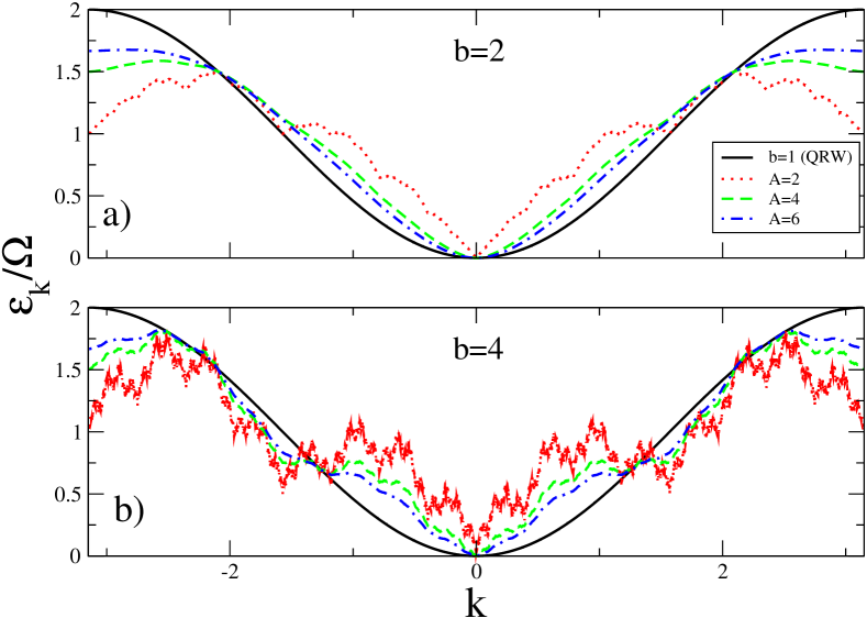
Figure 1: Plot of $\mathcal{E}_{k}(b,\mathcal{A)}/\Omega$, the continuous energy eigenvalue of Hamiltonian (1) as a function of the Fourier number $k$ in the first Brillouin zone (reciprocal to the Wannier lattice index). In (a) and (b) the straight lines correspond to the tight-binding case, i.e., the QRW model ($b=1$). The other lines (dotted, slashed and dotted-slashed) correspond to the QLW for different values of Weierstrass’ parameters: $b(=2,4),\mathcal{A}(=2,4,6)$. For large values of the Weierstrass’ rate $b/\mathcal{A}>1$ the non-differentiable structure of $\mathcal{E}_{k}(b,\mathcal{A)}$ is clearly visible as was predicted from the scaling (6) and also from Eq. (8).

Here it is important to note the difference with the classical characteristic function of the Weierstrass random walk (discrete space Levy flight Mandelbrot ; HSM81 ; MSh94 ; slesinger ; libro ). In the classical walk the condition to have an infinite mean square displacement per step is $b^{2}/\mathcal{A}>1$ (because the second moment is given by the second derivative of $\lambda(k)$). Then when clustering occurs, the number of subclusters within a distance $b^{n}$ of the origin is, on average, $\mathcal{A}^{n}$. Note that for the classical walk, the characteristic function of the Weierstrass walk is non-differentiable when $0<\mu<1$. Then it is possible to call to the value $\mu=\ln\mathcal{A}/\ln b$ the Hausdorff-Besicovitch dimension of the set of sites visited by a classical walk slesinger ; HMSch . In quantum mechanics a similar analysis could be done in the context of the Schödringer-Langevin picture jpa , i.e., without using the density matrix.

We want to remark that if $\mu<1$ ($b>A$) the eigenenergy $\mathcal{E}_{k}(b,\mathcal{A})$ is non-differentiable and the DOS is not well defined. A rigorous calculus based on the scaling properties (6) of the eigenenergy leads to the conclusion that the record of $\mathcal{E}_{k}(b,\mathcal{A})$ as a function of $k$, for $b$ above the critical value $b>A$, is a self-affine function. In fact, a fractal dimension can be measured (for example) by using the Box-counting technique and the prediction gives $D=2-\mu$ for $0<\mu<1$ Mandelbrot2 ; Feder ; libro . An alternative technique based in the analysis properties of the zero crossing HIJ-2007 has recently been reported to be suitable to characterizes processes that are continuous, but the derivative has fractal properties. Interestingly many years ago these processes were termed “subfractals” J1981 .

Note that we are assuming integer values for $b$ to avoid non-commensurability problems for the walk in the associated discrete infinite dimensional Hilbert space $\mathbf{H}$ of lattice parameter $\epsilon=1$ (at the end of appendix B we present some discussion on the case when the lattice parameter $\epsilon$ goes to the continuous limit).

II.1 The Quantum Master Equation for the quantum Levy walk

Concerning the quantum bath (see appendix A for details), we will assume that the thermal bath $\mathcal{B}$ is an infinite set of oscillators, and that the interaction with the phonon bath causes the free particle to jump either to the right or to the left. Thus we consider the operators $V_{\beta}$ appearing in the interaction Hamiltonian (47) to be proportional to the Weierstrass shift operators $a$ and $a^{{\dagger}}$ defined in Eq. (4). In the present paper we will study a particular coupling with the heat bath, nevertheless going back to appendices A, B and C it is straightforward to write down the QME considering any other type of coupling. For example: if $V_{\beta}\propto a-a^{{\dagger}}$ we can model an interaction that in the continuos limit (lattice parameter going to zero) coupled the velocity of the free particle with the heat bath.

Taking into account that $[a^{{\dagger}},a]=0$ we trivially get that in the Heisenberg representation Weierstrass’s shift operator does not have a time evolution, i.e.,:

$$V_{\beta}(-\tau)\equiv\exp(-i\tau H_{S}/\hbar)V_{\beta}\exp(i\tau H_{S}/\hbar)=V_{\beta}(0).$$

This result ultimately will lead to the fact that the Kossakowski-Lindblad (KL) generator kossa ; lindblad will be completely positive jpa . Thus, using Eqs. (48) and (49) in (42), we can write the Quantum Master Equation (QME), for the reduced density matrix $\rho$, in the form (see (C) in appendix C)

$$\dot{\rho}=\frac{-i}{\hbar}\left[H_{eff},\rho\right]+\frac{\pi\alpha}{4\beta\hbar}\left(2a\rho a^{{\dagger}}-a^{{\dagger}}a\rho-\rho a^{{\dagger}}a\right)+\frac{\pi\alpha}{4\beta\hbar}\left(2a^{{\dagger}}\rho a-aa^{{\dagger}}\rho-\rho aa^{{\dagger}}\right).$$ (9)

Here $\alpha>0$ is the dissipative constant and $\beta$ the inverse of the temperature of the bath.

Note that in the case $b\neq 1$ we have $a^{{\dagger}}a\neq\mathbf{1}$ (see appendix B) therefore the effective Hamiltonian has a non-trivial contribution:

$$H_{eff}=H_{S}-\hbar\omega_{c}a^{{\dagger}}a,\quad\omega_{c}>0.$$ (10)

The effective Hamiltonian can also be diagonalized in the Fourier basis, therefore we get

$$\left\langle k_{1}\right|H_{eff}\left|k_{2}\right\rangle = \left[\mathcal{E}_{k_{1}}(b,\mathcal{A)}\ -\hbar\omega_{c}\left(\frac{\mathcal{A-}1}{\mathcal{A}}\right)^{2}\sum\limits_{n_{2},n_{1}=0}^{\infty}\frac{\cos k_{1}\left(b^{n_{2}}-b^{n_{1}}\right)}{\mathcal{A}^{n_{1}+n_{2}}}\right]\delta\left(k_{1}-k_{2}\right)$$ (11)

$$\equiv \mathrm{E}_{k_{1}}(b,\mathcal{A)}\ \delta\left(k_{1}-k_{2}\right),$$

where we have used (53) and $\mathcal{E}_{k_{1}}(b,\mathcal{A)}$ is given in (5). Note that $\hbar\omega_{c}$ is an upper bound energy which is characteristic of the Ohmic approximation caldeira , (see (62) in the appendix C). In figure 2 we have plotted $\mathrm{E}_{k}(b,\mathcal{A)}$ for several values of Weierstrass’ parameters $b,\mathcal{A}$, in this plot it can be seen that the effective eigenenergy associated to the Hamiltonian (10) has larger fluctuations than $\mathcal{E}_{k_{1}}(b,\mathcal{A)}$ the eigenenergy associated to the naked Levy walk Hamiltonian.

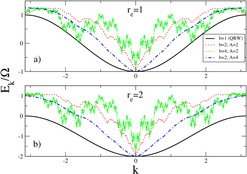
Figure 2: Plot of $\mathrm{E}_{k_{1}}(b,\mathcal{A)}/\Omega$, the continuous energy eigenvalue of the effective Hamiltonian (10) as a function of the Fourier number $k$ in the first Brillouin zone. In (a) the energy rate is $r_{e}=\hbar\omega_{c}/\Omega=1$, and in (b) is $r_{e}=2$. The straight lines correspond to the tight-binding case ($b=1$). Other lines (dotted, slashed and dotted-slashed) correspond to the QLW model for different values of Weierstrass’ parameters $b(=2,4),\mathcal{A}(=2,4)$. The physical meaning of the contribution $\hbar\omega_{c}a^{{\dagger}}a$ in the effective Hamiltonian $H_{eff}$ can be thought as increasing the multiplicity of the hopping structure, see (52). For $b>A$ and large values of the rate $r_{e}$ the amplitude of the non-differential structure get larger.

When $b=1$ (the QRW case) the effective Hamiltonian only introduces a trivial constant because $\lim_{b\rightarrow 1}a^{{\dagger}}a\rightarrow\mathbf{1}$. Therefore, for $b=1$ the KL generator has a very simple expression, form (9) the QME results vK95 ; MOC-CH97

$$L\left[\rho\right]=\frac{-i}{\hbar}\left[H_{S},\rho\right]+\frac{\pi\alpha}{2\beta\hbar}\left(a\rho a^{{\dagger}}+a^{{\dagger}}\rho a\right)-\frac{\pi\alpha}{\beta\hbar}\rho\qquad\text{if\qquad}b=1,$$

the group $\pi\alpha/2\beta\hbar$ can be called the diffusion constant $D$ and is given in units of [time]^-1 because the lattice parameter is dimensionless. The case $D\rightarrow\infty$ corresponds to the high temperature limit, see appendix C.

II.2
On the second moment of the quantum Levy walk

From the QME (9) we can obtain the dynamics of any operator, in particular here we are interested in the evolution of the dispersion of the position operator $\mathbf{q}$, which in the Wannier basis has the matrix elements:

$$\left\langle l_{1}\right|\mathbf{q}\left|l_{2}\right\rangle=l\delta_{l_{1},l_{2}},$$ (12)

note that $\mathbf{q}$ is defined as a dimensionless position operator. In the $\left|l\right\rangle$ representation it is possible to see that the thermal mean-value time-evolution of the first and second quantum moments can be written in the form:

$$\frac{d}{dt}\left\langle\mathbf{q}(t)\right\rangle = \frac{d}{dt}Tr\left\{\mathbf{q}(t)\rho(0)\right\}=Tr\left\{\mathbf{q}\dot{\rho}(t)\right\}$$

$$= \frac{-i}{\hbar}Tr\left\{\rho\left[\mathbf{q},H_{eff}\right]\right\}$$

$$\frac{d}{dt}\left\langle\mathbf{q}^{2}(t)\right\rangle = Tr\left\{\mathbf{q}^{2}\dot{\rho}(t)\right\}$$

$$= \frac{-i}{\hbar}Tr\left\{\rho\left[\mathbf{q}^{2},H_{eff}\right]\right\}+\frac{\pi\alpha}{\beta\hbar}\left(\frac{\mathcal{A-}1}{\mathcal{A}}\right)^{2}\sum_{n_{1},n_{2}=0}^{\infty}\sum_{l=-\infty}^{\infty}\frac{b^{n_{1}}b^{n_{2}}}{\mathcal{A}^{n_{1}+n_{2}}}\left\langle l\right|\rho(t)\left|l-b^{n_{1}}+b^{n_{2}}\right\rangle.$$

Setting $b=1$ in (II.2) and (II.2), i.e., in the limit of the usual QRW, we can write in the Heisenberg representation:

$$\frac{d}{dt}\mathbf{q}(t) = \frac{-i}{\hbar}\left[\mathbf{q},H_{S}\right]\qquad if\qquad b=1,$$ (15)

$$\frac{d}{dt}\mathbf{q}^{2}(t) = \frac{-i}{\hbar}\left[\mathbf{q}^{2},H_{S}\right]+\frac{\pi\alpha}{\beta\hbar}\qquad if\qquad b=1.$$ (16)

These equations can easily be solved. Using that $\left[\mathbf{q},H_{S}\right]=\frac{\Omega}{2}\left(a-a^{{\dagger}}\right)$ (see appendix B), and that $a(t)=a(0),a^{{\dagger}}(t)=a^{{\dagger}}(0)$ we get for the time evolution of the position operator:

$$\mathbf{q}(t)=\frac{-i\Omega}{2\hbar}\left(a-a^{{\dagger}}\right)t+\mathbf{q}(0)\qquad if\qquad b=1.$$

In the same way, the variance of the QRW (the NN walk model) can be calculated giving: $\left\langle\mathbf{q}(t)^{2}\right\rangle-\left\langle\mathbf{q}(t)\right\rangle^{2}=\frac{1}{2}\left(\frac{\Omega t}{\hbar}\right)^{2}+2Dt$, with $2D\equiv$ $\frac{\pi\alpha}{\beta\hbar}$, which is the expected dissipative result MOC-CH97 ; kampen ; libro ; vK95 . From (15) and (16) it is possible to see that von Neumann’s term gives a contribution of the form $\propto t^{2}$ for the time-evolution of the second moment, this is a well known quantum result Blumen08a , see eq. (23) for a general discussion. The dissipative contribution comes from the interaction with the bath $\mathcal{B}$, giving the classical diffusive behavior $\propto t$.

From (II.2) and due to the coherent dynamics involved through the time-evolution of the off-diagonal elements $\left\langle l\right|\rho(t)\left|l-b^{n_{1}}+b^{n_{2}}\right\rangle$, it is not simple to realize what will be the dynamics in the general case when $b\neq 1$. But in principle any higher moments of $\mathbf{q}(t)$ can also be analyzed in the same way from our QME (9).

Let us now analyze the case $b\neq 1$. In this case the interaction with $\mathcal{B}$ produces long-range hopping, and consistently a non-trivial quantum decoherence phenomenon. The dissipative term of (II.2), can also be written in the form:

$$\frac{\pi\alpha}{\beta\hbar}\left(\frac{\mathcal{A-}1}{\mathcal{A}}\right)^{2}\sum_{n_{1},n_{2}=0}^{\infty}\left(\frac{b}{\mathcal{A}}\right)^{n_{1}+n_{2}}\sum_{l=-\infty}^{\infty}\left\langle l+b^{n_{1}}\right|\rho(t)\left|l+b^{n_{2}}\right\rangle.$$ (17)

We can explicitly calculate this contribution by going to the Fourier representation. First of all, here we will assume that the initial condition for the reduced density matrix was prepared in a pure Wannier state: $\rho(0)=\left|l_{0}\right\rangle\left\langle l_{0}\right|$, so

$$\rho(0)_{k_{1},k_{2}}\equiv\left\langle k_{1}\right|\rho(0)\left|k_{2}\right\rangle=\frac{1}{2\pi}\exp\left(-i(k_{1}-k_{2})l_{0}\right),$$ (18)

thus $\left\langle k\right|\rho(0)\left|k\right\rangle=\frac{1}{2\pi}$. On the other hand, from (9) is possible to see that $\frac{d}{dt}\left\langle k\right|\rho(t)\left|k\right\rangle=0$ therefore $\left\langle k\right|\rho(t)\left|k\right\rangle=\frac{1}{2\pi},\forall t$, (see next section). Now going back to (17) we can write:

$$(\ref{non-D}) = \frac{\pi\alpha}{\beta\hbar}\left(\frac{\mathcal{A-}1}{\mathcal{A}}\right)^{2}\int\int dk_{1}dk_{2}\sum_{n_{1},n_{2}=0}^{\infty}\left(\frac{b}{\mathcal{A}}\right)^{{}^{n_{1}+n_{2}}}\sum_{l=-\infty}^{\infty}\left\langle l+b^{n_{1}}\right|\left.k_{1}\right\rangle\left\langle k_{1}\right|\rho(t)\left|k_{2}\right\rangle\left\langle k_{2}\right.\left|l+b^{n_{2}}\right\rangle$$

$$= \frac{\pi\alpha}{\beta\hbar}\left(\frac{\mathcal{A-}1}{\mathcal{A}}\right)^{2}\int\int dk_{1}dk_{2}\sum_{n_{1},n_{2}=0}^{\infty}\left(\frac{b}{\mathcal{A}}\right)^{{}^{n_{1}+n_{2}}}e^{ib^{n_{1}}k_{1}-ib^{n_{2}}k_{2}}\left\langle k_{1}\right|\rho(t)\left|k_{2}\right\rangle\sum_{l=-\infty}^{\infty}\frac{e^{i(k_{1}-k_{2})l}}{2\pi}$$

$$= \frac{\pi\alpha}{\beta\hbar}\left(\frac{\mathcal{A-}1}{\mathcal{A}}\right)^{2}\sum_{n_{1},n_{2}=0}^{\infty}\left(\frac{b}{\mathcal{A}}\right)^{{}^{n_{1}+n_{2}}}\int_{-\pi}^{\pi}dk_{1}e^{i(b^{n_{1}}-b^{n_{2}})k_{1}}\left\langle k_{1}\right|\rho(t)\left|k_{1}\right\rangle$$

$$= \frac{\pi\alpha}{\beta\hbar}\left(\frac{\mathcal{A-}1}{\mathcal{A}}\right)^{2}\sum_{n_{1},n_{2}=0}^{\infty}\left(\frac{b}{\mathcal{A}}\right)^{{}^{n_{1}+n_{2}}}\frac{1}{2\pi}\int_{-\pi}^{\pi}dk_{1}e^{i(b^{n_{1}}-b^{n_{2}})k_{1}}$$

$$= \frac{\pi\alpha}{\beta\hbar}\left(\frac{\mathcal{A-}1}{\mathcal{A}}\right)^{2}\sum_{n_{1},n_{2}=0}^{\infty}\left(\frac{b}{\mathcal{A}}\right)^{{}^{n_{1}+n_{2}}}\frac{\sin(b^{n_{1}}-b^{n_{2}})\pi}{(b^{n_{1}}-b^{n_{2}})\pi},$$

noting that we have assumed $b=\mbox{integer}$ we can write:

$$(\ref{non-D}) = \frac{\pi\alpha}{\beta\hbar}\left(\frac{\mathcal{A-}1}{\mathcal{A}}\right)^{2}\left(\frac{\mathcal{A}^{2}}{\mathcal{A}^{2}-b^{2}}+\sum_{n_{1}\neq n_{2}}^{\infty}\left(\frac{b}{\mathcal{A}}\right)^{{}^{n_{1}+n_{2}}}\frac{\sin(b^{n_{1}}-b^{n_{2}})\pi}{(b^{n_{1}}-b^{n_{2}})\pi}\right)$$ (22)

$$= \left\{\begin{array}[]{c}\!\frac{\pi\alpha}{\beta\hbar},\quad if\quad b=1,\\ \qquad\frac{\pi\alpha}{\beta\hbar}\frac{\left(\mathcal{A-}1\right)^{2}}{\mathcal{A}^{2}-b^{2}},\quad if\quad\mathcal{A}>1,b(\text{integer})<\mathcal{A},\\ \!\infty,\quad if\quad b>\mathcal{A}.\qquad\qquad\blacksquare\end{array}\right.$$

The expression (22) shows that it is only in the case when $b>$ $\mathcal{A}$ that a divergent behavior for the thermal second moment of the QLW, $\left\langle\mathbf{q}^{2}(t)\right\rangle,$ can arise. This quantum result is quite different from the classical clustering Levy flight counterpart ($b^{2}>\mathcal{A}$) Mandelbrot ; HSM81 ; MSh94 ; slesinger ; libro .

The explicit solution of $\left\langle\mathbf{q}^{2}(t)\right\rangle$ can alternatively be obtained calculating $Tr\left[\mathbf{q}^{2}\rho(t)\right]$ (this is done in appendix D):

$$\left\langle\mathbf{q}^{2}(t)\right\rangle=\left\{\begin{array}[]{c}\frac{1}{2}\left(\frac{\Omega}{\hbar}t\right)^{2}+\frac{\pi\alpha}{\beta\hbar}t+l_{0}^{2},\quad if\quad\mathcal{A}>1,b=1,\\ \\ \frac{\left(\mathcal{A-}1\right)^{2}}{\mathcal{A}^{2}-b^{2}}\left(\frac{1}{2}\frac{\Omega^{2}}{\hbar^{2}}t^{2}+\frac{2\omega_{c}^{2}\left(b-1\right)^{2}}{\left(1-1/\mathcal{A}^{2}\right)\left(1-b/\mathcal{A}^{2}\right)^{2}}t^{2}+\frac{\pi\alpha}{\beta\hbar}t\right)+l_{0}^{2},\quad if\quad\mathcal{A}>1,b<\mathcal{A}.\end{array}\right.$$ (23)

By taking the limit of null dissipation, i.e., $\alpha=0$ we reobtain the quantum behavior $\left\langle\mathbf{q}^{2}(t)\right\rangle\propto t^{2}$ for $b<\mathcal{A}$, this result is in agreement with previous reports on the universal behavior of quantum walks with long-range steps Blumen08a .

We conclude this section noting that the quantum coherence enlarges the threshold (compared to the classical one) to have a finite second moment for the walk. For example, if $b=2,\mathcal{A}=3$ the classical second moment is not defined, but the thermal quantum average $\left\langle\mathbf{q}^{2}(t)\right\rangle$ is finite!

II.3 Time evolution of the density matrix

II.3.1
Off-diagonal relaxation

The QME (9) can be solved in the basis of the eigenvectors of $H_{S}$. Introducing the representation $\left|k\right\rangle$, and using that $\left\langle k_{1}\right|H_{eff}\left|k_{2}\right\rangle=\mathrm{E}_{k_{1}}\ \delta\left(k_{1}-k_{2}\right)$, with E${}_{k_{1}}\equiv\mathrm{E}_{k_{1}}(b,\mathcal{A})$ given in (11) we get (see appendix C):

$$\left\langle k_{1}\right|\dot{\rho}\left|k_{2}\right\rangle = \frac{-i}{\hbar}\left(\mathrm{E}_{k_{1}}-\mathrm{E}_{k_{2}}\right)\left\langle k_{1}\right|\rho\left|k_{2}\right\rangle$$ (24)

$$+\frac{\pi\alpha}{2\beta\hbar}\left(\frac{\mathcal{A-}1}{\mathcal{A}}\right)^{2}\sum_{n_{1},n_{2}=0}^{\infty}\frac{1}{\mathcal{A}^{n_{1}+n_{2}}}\left[2\cos\left(k_{1}b^{n_{1}}-k_{2}b^{n_{2}}\right)\right.$$

$$-\left.\cos k_{1}\left(b^{n_{1}}-b^{n_{2}}\right)-\cos k_{2}\left(b^{n_{1}}-b^{n_{2}}\right)\right]\left\langle k_{1}\right|\rho\left|k_{2}\right\rangle.$$

From (24) the general solution for the reduced density matrix is

$$\left\langle k_{1}\right|\rho(t)\left|k_{2}\right\rangle=\rho(0)_{k_{1}k_{2}}\ \exp\left(\mathcal{F}\left(k_{1},k_{2},b,\mathcal{A}\right)t\right),$$ (25)

with

$$\mathcal{F}\left(k_{1},k_{2},b,\mathcal{A}\right) \equiv \frac{i}{\hbar}\left[\Omega\frac{\mathcal{A-}1}{\mathcal{A}}\sum_{n=0}^{\infty}\frac{1}{\mathcal{A}^{n}}\left(\cos\left(b^{n}k_{1}\right)-\cos\left(b^{n}k_{2}\right)\right)\right.$$ (26)

$$+\left.\hbar\omega_{c}\left(\frac{\mathcal{A-}1}{\mathcal{A}}\right)^{2}\sum\limits_{n_{2},n_{1}=0}^{\infty}\frac{\cos k_{1}\left(b^{n_{2}}-b^{n_{1}}\right)}{\mathcal{A}^{n_{1}+n_{2}}}-\frac{\cos k_{2}\left(b^{n_{2}}-b^{n_{1}}\right)}{\mathcal{A}^{n_{1}+n_{2}}}\right]$$

$$+\frac{\pi\alpha}{2\beta\hbar}\left(\frac{\mathcal{A-}1}{\mathcal{A}}\right)^{2}\sum_{n_{1},n_{2}=0}^{\infty}\frac{1}{\mathcal{A}^{n_{1}+n_{2}}}\left[2\cos\left(k_{1}b^{n_{1}}-k_{2}b^{n_{2}}\right)\right.$$

$$-\left.\cos k_{1}\left(b^{n_{1}}-b^{n_{2}}\right)-\cos k_{2}\left(b^{n_{1}}-b^{n_{2}}\right)\right],$$

note that $\mathcal{F}\left(k,k,b,\mathcal{A}\right)=0.$

For the QRW (case $b=1$) the QME (24) reduces to a simpler form

$$\left\langle k_{1}\right|\dot{\rho}\left|k_{2}\right\rangle=\left[\frac{-i}{\hbar}\left(\mathrm{E}_{k_{1}}-\mathrm{E}_{k_{2}}\right)+\frac{\pi\alpha}{\beta\hbar}\left(\cos\left(k_{1}-k_{2}\right)-1\right)\right]\left\langle k_{1}\right|\rho\left|k_{2}\right\rangle,$$

where $\mathrm{E}_{k}=\Omega\left\{1-\cos k\right\}-\hbar\omega_{c}.$ Note that in the NN case, the off-diagonal relaxation of the element $\rho_{k,0}(t)$ (from the homogeneous Fourier mode) is just controlled by a trivial trigonometric function:

$$\mathcal{F}\left(k,0,b=1,\mathcal{A}\right)=-\left[i\frac{\Omega}{\hbar}+\frac{\pi\alpha}{\beta\hbar}\right]\left(1-\cos k\right).$$

This result resembles the relaxation of the Fourier modes of a classical one dimensional ordered walk with a diffusion coefficient $2D=\frac{\pi\alpha}{\beta\hbar}$ (see appendix E). Note however that in quantum mechanic the relaxation of the initial position is controlled by a double Fourier integral, so we cannot expect the same long-time asymptotic behavior as in classic (see next sections for details).

II.3.2 Diagonal relaxation

In general for $b\geq 1,$ by putting $k_{1}=k_{2}$ in (24), we see that the diagonal elements $\rho_{kk}(t)$ remain constant in time:

$$\frac{d}{dt}\left\langle k\right|\rho\left|k\right\rangle=0.$$ (27)

This result tell that even when there is a decoherence in the off-diagonal elements of the density matrix, the probability distribution of the Fourier modes is invariant in time. The physical interpretation of this fact can be understood by noting that the thermal average of the kinetic energy is constant in time. As we mention before this is a consequence of the general form of the shift operators (2) and (3).

To prove this fact for the Weierstrass model, we first define a pseudo-momentum operator:

$$\mathbf{p}\equiv\frac{m}{i\hbar}\left[\mathbf{q},H_{S}\right],$$ (28)

where $m$ represents the mass of our free particle in the lattice. From (54) it is simple to see that $\mathbf{p}$ is diagonal in the Fourier basis $\mathbf{p}\left|k\right\rangle=\mathbf{p}_{k}\left|k\right\rangle$, i.e.,

$$\left\langle k_{1}\right|\mathbf{p}\left|k\right\rangle = \frac{m\Omega}{\hbar}\left(\frac{\mathcal{A-}1}{\mathcal{A}}\right)\sum_{n}\left(\frac{b}{\mathcal{A}}\right)^{n}\sin\left(kb^{n}\right)\delta\left(k-k_{1}\right)$$

$$\equiv \delta\left(k-k_{1}\right)\mathbf{p}_{k}.$$

Once again the eigenvalue $\mathbf{p}_{k}$ is well defined only below the threshold $b<\mathcal{A}$.

Assuming the system was prepared in the pure state: $\rho(0)=\left|l_{0}\right\rangle\left\langle l_{0}\right|$, the thermal average of the pseudo-momentum gives $\left\langle\mathbf{p}(t)\right\rangle=0,\forall t$, and for $\left\langle\mathbf{p}^{2}(t)\right\rangle$ we get

$$\left\langle\mathbf{p}^{2}(t)\right\rangle = Tr\left[\mathbf{p}^{2}\rho(t)\right]=\int_{-\pi}^{\pi}dk\int_{-\pi}^{\pi}dk_{1}\left\langle k\right|\mathbf{p}^{2}\left|k_{1}\right\rangle\left\langle k_{1}\right|\rho(t)\left|k\right\rangle$$

$$= \int_{-\pi}^{\pi}dk\int_{-\pi}^{\pi}dk_{1}\ \left(\mathbf{p}_{k}\right)^{2}\delta\left(k_{1}-k\right)\left\langle k_{1}\right|\rho(t)\left|k\right\rangle$$

$$= \frac{1}{2\pi}\int_{-\pi}^{\pi}dk\ \left(\mathbf{p}_{k}\right)^{2}=\text{constant,}$$

where we have used that $\left\langle k\right|\rho(t)\left|k\right\rangle=\frac{1}{2\pi},\forall t.$ In general it is possible to prove that the thermal average of any observable which is diagonal in the Fourier basis, will be constant in time.

It is interesting to comment here that for the QRW (the NN case) the pseudo-momentum operator (28) is in fact a discrete version of the momentum, and can be written in the form (see appendix B)

$$\mathbf{p}\equiv\frac{\Omega m}{i\hbar 2}\left(a-a^{{\dagger}}\right),\qquad\text{if\qquad}b=1,$$

then it is simple to see that $\mathbf{\dot{p}}\equiv\frac{1}{i\hbar}\left[\mathbf{p},H_{S}\right]=0$, so the discrete momentum in the Heisenberg representation is constant in time. The “lattice” commutation relation between the position and the momentum gives

$$\left[\mathbf{q},\mathbf{p}\right]\equiv-\frac{\Omega m}{i\hbar 2}\left(a+a^{{\dagger}}\right),\qquad\text{if\qquad}b=1.$$

Thus in the continuous limit (taking the lattice parameter $\epsilon\rightarrow 0$, see appendix B) we reobtain the usual commutation relation $\left[\mathbf{q},\mathbf{p}\right]\equiv i\hbar\mathbf{1}$, MOC-CH97 .

II.3.3 Quantum decoherence from a pure state

In order to study the quantum decoherence due to the interaction with the thermal bath $\mathcal{B}$, we propose here to analyze the time evolution of the density matrix assuming that at time $t=0$ the system was prepared in a pure state: $\rho(0)=\left|l_{0}\right\rangle$ $\left\langle l_{0}\right|$. Then the quantum probability to be at site $l$ at time $t$ is given by

$$\left\langle l\right|\rho(t)\left|l\right\rangle = \int_{-\pi}^{\pi}dk_{1}\int_{-\pi}^{\pi}dk_{2}\left\langle l\right.\left|k_{1}\right\rangle\left\langle k_{1}\right|\rho(t)\left|k_{2}\right\rangle\left\langle k_{2}\right|\left.l\right\rangle$$

$$= \frac{1}{2\pi}\int_{-\pi}^{\pi}dk_{1}\int_{-\pi}^{\pi}dk_{2}\exp\left[i\left(k_{1}-k_{2}\right)l\right]\left\langle k_{1}\right|\rho(t)\left|k_{2}\right\rangle$$

$$= \left(\frac{1}{2\pi}\right)^{2}\int_{-\pi}^{\pi}dk_{1}\int_{-\pi}^{\pi}dk_{2}\exp\left[i\left(k_{1}-k_{2}\right)(l-l_{0})\right]\exp\left(\mathcal{F}\left(k_{1},k_{2},b,\mathcal{A}\right)t\right).$$

Calling $(l-l_{0})=\Delta l$ the distance form the initial condition, we can plot the probability $\mathit{P}(\Delta l,t)\equiv\left\langle l\right|\rho(t)\left|l\right\rangle$ as a function of $\Delta l$ for different values of time $t$, and Weierstrass’ parameters $b,\mathcal{A}$. Note that $\mathit{P}(\Delta l,t)\leq 1$ as expected because the density matrix is well normalized $\sum_{l}\left\langle l\right|\rho(t)\left|l\right\rangle=1,\forall t\neq\infty$, as can easily be checked from (II.3.3). In figure 3 we plot $\mathit{P}(\Delta l,t)$ for different values of the frequency rates $r=\frac{\Omega}{\hbar}/D$, $r_{c}=\omega_{c}/D$ and Weierstrass’ parameters $b,\mathcal{A}$, the non diffusive characteristics of the profile $\mathit{P}(\Delta l,t)$ as well as its trimodality behavior can clearly be seen. This trimodality is the result of the combination between the non-diffusive characteristics (clustering) of the Levy walk (by increasing $b>A$) and the quantum oscillations (coherence by increasing $r>1,r_{c}>1$). All Fourier integrals were made using the numerical integration quadrature method numerical .

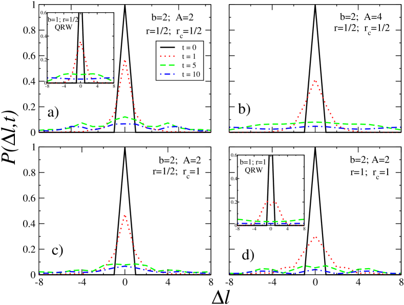
Figure 3: Plot of the position probability $\mathit{P}(\Delta l,t)$ when the system is prepared in the pure state $\rho(0)=\left|l_{0}\right\rangle\left\langle l_{0}\right|$ as a function of $\Delta l$ (dimensionless space difference $\Delta l\equiv l-l_{0}$), for several values of dimensionless time $t$ ($D$ is given in units of [time]^-1). In the insets we show the QRW case $(b=1)$, then it is possible to see that by increasing the frequency rate $r=\frac{\Omega}{\hbar}/D$ the quantum time-oscillations around $\Delta l=0$ persist longer before the profile spreads in a diffusive way. In figures (a)-(d) we show the same profile but for the QLW model $(b\neq 1)$ for $r=\frac{1}{2},1,$ two values of the Weierstrass’ rate $b/\mathcal{A}$ and frequency rate $r_{c}=\omega_{c}/D$.  For the QLW there is a non-trivial effective Hamiltonian (10), then we have to specify $r_{c}$ which is the dimensionless number comparing the Caldeira-Legget upper frequency caldeira against the diffusion coefficient. In (a), (d) and (c), we chose $b/\mathcal{A}=1$ then the trimodality of the profile is easily seen. In (a) for $r_{c}=\frac{1}{2}$ the non-diffusive behavior is more visible than in (c) for $r_{c}=1$, this trimodality behavior is enhanced by increasing the Weierstrass’ rate $b/\mathcal{A}>1$ and the frequency rate $r$. In (b) we chose $b/\mathcal{A}<1$ so the second moment of the $\mathit{P}(\Delta l,t)$ is finite, see (23), here the profile spreads but its non-diffusion characteristics is clearly visible.

From (II.3.3) we see that in quantum mechanic the relaxation of the initial position is controlled by a double integral:

$$\left\langle l_{0}\right|\rho(t)\left|l_{0}\right\rangle=\left(\frac{1}{2\pi}\right)^{2}\int_{-\pi}^{\pi}dk_{1}\int_{-\pi}^{\pi}dk_{2}\exp\left(\mathcal{F}\left(k_{1},k_{2},b,\mathcal{A}\right)t\right).$$

For the case $b=1$, i.e., the QRW, we can calculate analytically the long-time asymptotic behavior in the following way

$$\left\langle l_{0}\right|\rho(t)\left|l_{0}\right\rangle = \left(\frac{1}{2\pi}\right)^{2}\int_{-\pi}^{\pi}dk_{1}\int_{-\pi}^{\pi}dk_{2}\exp\left[\frac{-i}{\hbar}\left(\mathrm{E}_{k_{1}}-\mathrm{E}_{k_{2}}\right)+\frac{\pi\alpha}{\beta\hbar}\left(\cos\left(k_{1}-k_{2}\right)-1\right)\right]t$$

$$= \left(\frac{1}{2\pi}\right)^{2}\int_{-\pi}^{\pi}dk_{1}\int_{-\pi}^{\pi}dk_{2}\exp\left[\frac{i\Omega}{\hbar}\left(\cos k_{1}-\cos k_{2}\right)+\frac{\pi\alpha}{\beta\hbar}\left(\cos\left(k_{1}-k_{2}\right)-1\right)\right]t$$

$$= \left(\frac{1}{2\pi}\right)^{2}\int_{-\pi}^{\pi}e^{\frac{i\Omega}{\hbar}t\cos k_{1}}\ dk_{1}\int_{-\pi}^{\pi}e^{\frac{-i\Omega}{\hbar}t\cos k_{2}}\exp\left[\frac{\pi\alpha}{\beta\hbar}\left(\cos\left(k_{1}-k_{2}\right)-1\right)\right]t\ dk_{2}.$$

In the limit of $t\rightarrow\infty$ we can use the method of steepest descent MSP , so defining the parameter $r=\left.\frac{\Omega}{\hbar}\right/\frac{\pi\alpha}{2\beta\hbar}$ it is possible to see that for $r\neq 0$ each Fourier integral introduces a factor $1/\sqrt{rt}$, thus the relaxation (in one dimension) goes like $\propto 1/rt$. On the other hand, if $r=0$ (infinite temperature limit) it is also possible to see analytically that the dominant contribution in the double integral comes from a small area near $k_{1}=k_{2}$, then we get for the quantum asymptotic behavior: $\propto 1/\sqrt{t}$, like in a classic random walk (see appendix E).

In general for $b\neq 1$ another alternative to study the quantum decoherence, is to evaluate some correlation function associated to the interference measurement phenomena. This can be done by analyzing the localization probability $\left\langle l_{0}\right|\rho(t)\left|l_{0}\right\rangle$. From the general expression for the density matrix, $\rho(t)$, in an arbitrary basis $\left|\phi_{j}\right\rangle$, we have

$$\rho(t)=\sum_{i\neq j}C_{i}(t)C_{j}^{\ast}(t)\ \left|\phi_{i}\right\rangle\left\langle\phi_{j}\right|+\sum_{j}\left|C_{j}(t)\right|^{2}\ \left|\phi_{j}\right\rangle\left\langle\phi_{j}\right|,$$

then we may conclude that $\sum_{j}\left|C_{j}(t)\right|^{2}\ \left|\left\langle\phi_{j}\right|\left.l_{0}\right\rangle\right|^{2}$ represents the classical probability mixture to measure the localization at time $t$. We can take into account the relaxation of the quantum interference, from the pure state $\rho(0)=\left|l_{0}\right\rangle$ $\left\langle l_{0}\right|$, as follows: the probability to measure at time $t$ the particle at the initial position is from (II.3.3):

$$\left\langle l_{0}\right|\rho(t)\left|l_{0}\right\rangle = \left(\frac{1}{2\pi}\right)^{2}\int_{-\pi}^{\pi}dk_{1}\int_{-\pi}^{\pi}dk_{2}\left[1-\delta\left(k_{1}-k_{2}\right)+\delta\left(k_{1}-k_{2}\right)\right]\exp\left(\mathcal{F}\left(k_{1},k_{2},b,\mathcal{A}\right)t\right)$$

$$= \left(\frac{1}{2\pi}\right)^{2}\int_{-\pi}^{\pi}dk_{1}\int_{-\pi}^{\pi}dk_{2}\left[1-\delta\left(k_{1}-k_{2}\right)\right]\exp\left(\mathcal{F}\left(k_{1},k_{2},b,\mathcal{A}\right)t\right)$$

$$+\left(\frac{1}{2\pi}\right)^{2}\int_{-\pi}^{\pi}dk_{1}\exp\left(\mathcal{F}\left(k_{1},k_{1},b,\mathcal{A}\right)t\right).$$

Thus using that $\exp\left(\mathcal{F}\left(k_{1},k_{1},b,\mathcal{A}\right)t\right)=1$, we see that the quantum interference is characterized by the localized correlation function $\chi(t)=\left\langle l_{0}\right|\rho(t)\left|l_{0}\right\rangle-\frac{1}{2\pi},$ i.e.,

$$\chi(t)=\left(\frac{1}{2\pi}\right)^{2}\int_{-\pi}^{\pi}dk_{1}\int_{-\pi}^{\pi}dk_{2}\exp\left(\mathcal{F}\left(k_{1},k_{2},b,\mathcal{A}\right)t\right)-\frac{1}{2\pi}.$$ (33)

In figure 4 we have plotted the localized correlation $\chi(t)$ as a function of time for different values of Weierstrass’ parameters $b,\mathcal{A}$, and for several frequency rates $r,r_{c}$ characterizing different energy regimes in the QME. In this figure the long-time coherence of $\chi(t)$ for the QLW can be compared against the diffusive decoherence corresponding to the QRW case, i.e., $\propto 1/t$. On the other hand, only in the infinite temperature limit $r\rightarrow 0$ the classical behavior $\propto 1/\sqrt{t}$ is reobtained (see Appendix E). There is some numerical evidence that $\chi(t)$ for the QLW is in fact bounded from above $\propto 1/\sqrt{t}$, and its long-time wavy behavior is the signature of the slow decoherence due to the scale-free hopping structure.

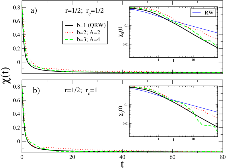
Figure 4: Plot of the localized correlation $\chi(t)$ for the QLW as a function of dimensionless time $t$ when the system is prepared in the pure state $\rho(0)=\left|l_{0}\right\rangle\left\langle l_{0}\right|$. The function $\chi(t)$ is plotted with $r=\frac{1}{2}$ for two values of Weierstrass’ rate $b/\mathcal{A}$ and frequency rate $r_{c}$. The insets show the log-log asymptotic behavior of $\chi_{0}(t)\equiv\chi(t)+\frac{1}{2\pi}$ against the QRW decay $\propto 1/t$ (wide straight line), also in the inset we have plotted (thin straight line) the classical RW localized probability $P_{0}(t)\propto 1/\sqrt{t}$, see (73). The long-time coherent behavior of $\chi(t)$ for the QLW is much more visible for large values of $r_{c}$. Note that if $r\neq 0$ none of the cases: QLW or the QRW behave asymptotically like a classical 1D walk (see appendix E for details). The localized quantum correlation $\chi(t)$ is bounded from above $\propto 1/\sqrt{t}$ and its wavy behavior for long-time (shown in the inset) is the signature of the slow decoherence due to Levy’s hopping structure.

In order to study the decoherence of a pure state due to the interaction with the thermal bath $B$, we propose here to analyze the time evolution of $Tr\left[\rho^{2}\right]$, this function is some time called the quantum purity. Assuming that at time $t=0$ the system was prepared in the Wannier pure state $\rho(0)=\left|l_{0}\right\rangle$ $\left\langle l_{0}\right|$, the quantum purity is given by

$$Tr\left[\rho(t)^{2}\right] = \int_{-\pi}^{\pi}dk_{1}\int_{-\pi}^{\pi}dk_{2}\left\langle k_{1}\right|\rho(t)\left|k_{2}\right\rangle\left\langle k_{2}\right|\rho(t)\left|k_{1}\right\rangle$$

$$= \left(\frac{1}{2\pi}\right)^{2}\int_{-\pi}^{\pi}dk_{1}\int_{-\pi}^{\pi}dk_{2}\exp\left[\mathcal{F}\left(k_{1},k_{2},b,\mathcal{A}\right)+\ \exp\mathcal{F}\left(k_{2},k_{1},b,\mathcal{A}\right)\right]t.$$

Introducing the definition of the rates $r,r_{c}$ in the explicit expression of $F\left(k_{1},k_{2},b,\mathcal{A}\right)$, from (26) we can see that

$$Tr\left[\rho(t)^{2}\right]=\left(\frac{1}{2\pi}\right)^{2}\int_{-\pi}^{\pi}dk_{1}\int_{-\pi}^{\pi}dk_{2}\ \exp\left\{\left.\mathcal{F}\left(k_{1},k_{2},b,\mathcal{A}\right)\right|_{r=r_{c}=0}\ 2Dt\right\}.$$ (34)

Thus the time can be rescaled in unit of the diffusion constant $D$, we also see that the behavior of the purity will be similar to the localized correlation function $\chi(t)$ but subtracting the quantum time-dependent oscillations, this is so because $F\left(k_{1},k_{2},b,\mathcal{A}\right)$ is evaluated at $r=r_{c}=0$, compare with (33). In figure 5 we show $Tr\left[\rho(t)^{2}\right]$ in a log-log plot for different values of Weierstrass’ parameters $b,A$. From this plot the non-trivial long tail behavior of the QLW can clearly be compared against the QRW case. For the case $b=1$ (the NN walks) and using the method of the steepest descent MSP from (34) is it possible to prove that the asymptotic behavior of the purity for the QRW is $\propto 1/\sqrt{Dt}$, this asymptotic regime is also shown (straight line) in figure 5. For the QLW $(b>1)$ we can see that the asymptotic behavior looks like $\propto 1/t^{\xi}$, where the exponent $\xi$ is a non-trivial function of Weierstrass’ parameters $b,A$. In the inset of this figure we also show the long-tail exponent $\xi$ versus the Weierstrass parameter $A$, here a transition in the behavior of $\xi$ for $b/A\lessgtr 1$ can be seen. From this inset it is also possible to see that if $A\gg 1$ the exponent $\xi$ goes to $0.5$ corresponding to the QRW case.

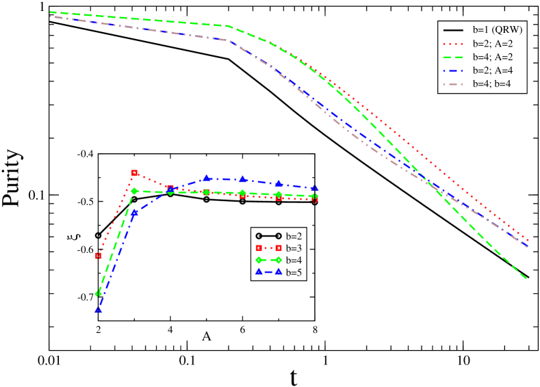
Figure 5: Log-log plot of the quantum purity $Tr\left[\rho^{2}\right]$ as a function of dimensionless time $t$ when the system is prepared in the pure state $\rho(0)=\left|l_{0}\right\rangle\left\langle l_{0}\right|$. The purity function is plotted for several values of Weierstrass’ rate $b/\mathcal{A}$. The purity for the QRW (straight line) shows the predicted long-time decoherent decay $\propto 1/\sqrt{t}$, see (34). The long-time asymptotic behavior for the QLW shows an asymptotic behavior like $\propto 1/t^{\xi}$ where the exponent $\xi$ depends on the Weierstrass’ parameters $b,\mathcal{A}$ in a non-trivial way, see inset.

II.3.4 Quantum decoherence from a coherent preparation in $\left|k\right\rangle$

Now we will study the relaxation from a coherente preparation in the Fourier bases. In order to simplify this analysis we adopt here the following initial preparation for the system

$$\rho(0)=\frac{1}{k_{c}}\int_{0}^{k_{c}}dk\int_{0}^{k_{c}}dk^{\prime}\left|k\right\rangle\left\langle k^{\prime}\right|,$$ (35)

where $k_{c}\leq\pi$ characterizes the initial uniform probability distribution in Fourier space. Therefore the mean-value of the Fourier modes appearing in the initial preparation is $\int_{-\pi}^{\pi}k\rho_{kk}(0)dk=k_{c}/2$. On the other hand, from (35) we get

$$\rho_{k_{1}k_{2}}(0) = \left\langle k_{1}\right|\rho(0)\left|k_{2}\right\rangle=\frac{1}{k_{c}}\int_{0}^{k_{c}}dk\int_{0}^{k_{c}}dk^{\prime}\delta\left(k_{1}-k\right)\delta\left(k^{\prime}-k_{2}\right)$$

$$= \frac{1}{k_{c}}\Theta\left(k_{c}-k_{1}\right)\Theta\left(k_{1}\right)\Theta\left(k_{c}-k_{2}\right)\Theta\left(k_{2}\right),$$

where $\Theta\left(z\right)$ is the step function. As indicated before the uniform initial probability distribution will be invariant in time $\rho_{kk}(0)=\frac{1}{k_{c}}\Theta\left(k_{c}-k\right)\Theta\left(k\right)$, and fulfills normalization:

$$\int_{-\pi}^{\pi}dk\rho_{kk}(0)=\frac{1}{k_{c}}\int_{-\pi}^{\pi}\Theta\left(k_{c}-k\right)\Theta\left(k\right)dk=1.$$

Therefore the probability $\left\langle l\right|\rho(t)\left|l\right\rangle$ will have a time dependent spreading, but with a well defined mean-velocity characterized by the Fourier value $k_{c}$. Using (II.3.4) as the initial preparation of the system, we get for the time-dependent probability to be at lattice site $l$

$$\left\langle l\right|\rho(t)\left|l\right\rangle = \int_{-\pi}^{\pi}dk_{1}\int_{-\pi}^{\pi}dk_{2}\left\langle l\right.\left|k_{1}\right\rangle\left\langle k_{1}\right|\rho(t)\left|k_{2}\right\rangle\left\langle k_{2}\right|\left.l\right\rangle$$ (37)

$$= \frac{1}{2\pi}\int_{-\pi}^{\pi}dk_{1}\int_{-\pi}^{\pi}dk_{2}\exp\left[i\left(k_{1}-k_{2}\right)l\right]\left\langle k_{1}\right|\rho(t)\left|k_{2}\right\rangle$$

$$= \frac{1}{2\pi k_{c}}\int_{0}^{k_{c}}dk_{1}\int_{0}^{k_{c}}dk_{2}\exp\left[i\left(k_{1}-k_{2}\right)l\right]\exp\left(\mathcal{F}\left(k_{1},k_{2},b,\mathcal{A}\right)t\right).$$

Note that at $t=0$ the initial distribution was delocalized in all the lattice according to:

$$\left\langle l\right|\rho(0)\left|l\right\rangle = \frac{1}{2\pi k_{c}}\int_{0}^{k_{c}}dk_{1}\int_{0}^{k_{c}}dk_{2}\exp\left[i\left(k_{1}-k_{2}\right)l\right]$$

$$= \frac{1}{\pi k_{c}l^{2}}\left(1-\cos k_{c}l\right),\qquad l\in\left(-\infty,+\infty\right).$$

In figure 6 we have plotted the probability $\left\langle l\right|\rho(t)\left|l\right\rangle$ from (37) as a function of the position $l$ for different values of time. The non-diffusive behavior as well as the reentrance phenomenon of the (driven) profile probability $\left\langle l\right|\rho(t)\left|l\right\rangle$ for the QLW can clearly be seen. What we call reentrance phenomenon is just the cooperative result of the clustering that occurs for $b>A$  and the quantum coherence. Classically the clustering is certain when $0<\mu<1$; only in the case $\mu\geq 1$ the walker ultimately returns to fill in any gaps in the set of sites visited and the clustering eventually disappears HMSch .

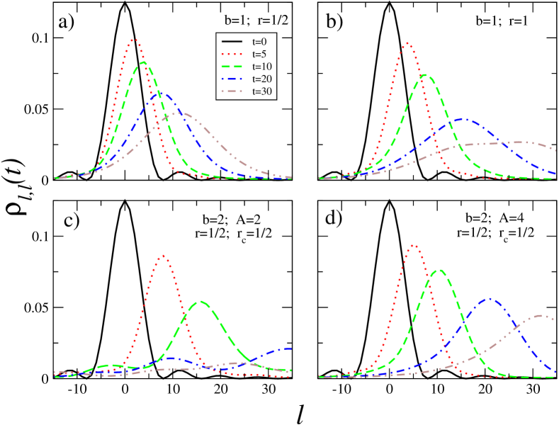
Figure 6: Plot of the probability $\rho_{l,l}(t)\equiv\left\langle l\right|\rho(t)\left|l\right\rangle$ as a function of lattice site $l$ for several values of dimensionless time $t$, Weierstrass’ rate $b/\mathcal{A}$, frequency rate $r$ and for $r_{c}=\frac{1}{2}$, when the system is prepared in a Fourier coherent state like in (35). The straight line corresponds to the profile at $t=0$ as is given in (II.3.4) for $k_{c}=\pi/4$. figures (a) and (b) correspond to the QRW $(b=1)$ for two values of rate $r$, the profile moves to the right with a thermal mean velocity as predicted in (39). In figure (c) it is possible to see the ”reentrance” of the probability to small values of $l$ for increasing time $(t=20)$, this phenomenon is due to the clustering of the visited sites and occurs above the critical value $b/\mathcal{A}>1.$

The agreement between the driven profile and the prediction associated to the pseudo-momentum is clearly visible from figure 6. Note that for the coherent preparation (35), the thermal mean value of the pseudo-momentum will be different from zero

$$\left\langle\mathbf{p}(t)\right\rangle = Tr\left[\mathbf{p}\rho(t)\right]=\int_{-\pi}^{\pi}dk\int_{-\pi}^{\pi}dk_{1}\left\langle k\right|\mathbf{p}\left|k_{1}\right\rangle\left\langle k_{1}\right|\rho(t)\left|k\right\rangle$$ (39)

$$= \int_{-\pi}^{\pi}dk\int_{-\pi}^{\pi}dk_{1}\ \mathbf{p}_{k}\delta\left(k_{1}-k\right)\left\langle k_{1}\right|\rho(t)\left|k\right\rangle$$

$$= \frac{1}{k_{c}}\int_{0}^{k_{c}}dk\ \mathbf{p}_{k}$$

$$= \frac{m\Omega}{\hbar k_{c}}\left(\frac{\mathcal{A-}1}{\mathcal{A}}\right)\sum_{n}\frac{1}{\mathcal{A}^{n}}\left[1-\cos\left(k_{c}b^{n}\right)\right],$$

where we have used (II.3.2). Interestingly taking $b=1$ in (39) we get that for the coherent initial preparation (35) the QRW has a thermal mean velocity characterized by $\left\langle\mathbf{p}(t)\right\rangle_{\text{QRW}}/m=\frac{\Omega}{\hbar k_{c}}\left[1-\cos\left(k_{c}\right)\right].$Therefore we may conclude that for the initial preparation (35), the driven profile of the QLW moves faster than the corresponding profile for the QRW, as can be seen from the following inequality:

$$\frac{\hbar k_{c}}{m\Omega}\left\langle\mathbf{p}(t)\right\rangle_{\text{QLW}}=\left(\frac{\mathcal{A-}1}{\mathcal{A}}\right)\sum_{n=0}\frac{1}{\mathcal{A}^{n}}\left[1-\cos\left(k_{c}b^{n}\right)\right]>\frac{\hbar k_{c}}{m\Omega}\left\langle\mathbf{p}(t)\right\rangle_{\text{QRW}}$$

Note from (39) that even when the eigenvalue $\mathbf{p}_{k}$, see (II.3.2), is not defined for $b>\mathcal{A}$, the double Fourier integral restores the regularity, i.e., the thermal mean-value of the pseudo-momentum $\left\langle\mathbf{p}(t)\right\rangle$ is well defined for any value of the Weierstrass parameters $b,\mathcal{A}$. Of course this is nothing more than the fact that by using the initial preparation (35) the probabilistic profile move to the right with a finite velocity. In the case $\mathcal{A}\gg 1$ the value of the thermal mean velocity goes to the one corresponding to the NN model.

III Discussions

In this work we have introduced the Weierstrass shift operators to build up the quantum master equation (also called Born-Markov equation) governing the quantum Levy walk process. We have started from the microscopic dynamics of a free particle, in a lattice, in interaction with a thermal phonon bath. The coupling with the heat bath was chosen proportional to shift operators (see (55) and (56)), but any type other coupling can be worked out using the recipes that we have write down in appendices A, B, C. Then the Kossakowski-Lindblad generator of the quantum semigroup, which is the starting point to analyze the positivity condition of the structure matrix, was built up. For the present model it was not necessary to apply Davies’s formalism (random phase approximation) to calculate the generator because Weierstrass’ shift operators, in the Heisenberg representation, are constant in time. This results in that the complete positivity condition of the generator was assured. The quantum Levy walk Hamiltonian shows for $b>\mathcal{A}$ that the DOS has a complex null-set inside the Brillouin zone, because the continuous eigenenergy $\mathcal{E}_{k}(b,\mathcal{A})$ is non-differentiable when $b/\mathcal{A}>1$. We proved that several physical objects show the signature of this singular characteristic. A rigorous calculus based on the scaling properties of the eigenenergy (6) leads to the conclusion that the record of $\mathcal{E}_{k}(b,\mathcal{A})$ as a function of $k$ shows a critical behavior for values $b>A$. In fact, the eigenenergy $\mathcal{E}_{k}(b,\mathcal{A})$ is self-affine with a (Box-counting) fractal dimension $D=2-\mu,$ for $0<\mu\equiv\ln\mathcal{A}/\ln b<1$.

The analytical solution of the quantum master equation has been found in the Fourier basis, see (25). In particular the evolution equation for the second moment (II.2), and its solution (23), has been calculated. Thus we prove that the thermal second moment is not divergent under the restriction $b<\mathcal{A}$, which is different when compared with the classical Weierstrass universality $b^{2}<\mathcal{A}$. The present quantum master equation can also be used to get information about higher moments and correlations of the quantum Levy walk process. The quantum decoherence has been characterized analyzing the probability to be in a lattice site considering different initial preparations for the system, i.e., we have worked out two different preparations for the reduced density matrix: a pure state in the Wannier basis, and a coherent preparation in the reciprocal Fourier basis. We have also examined the interference correlation function associated to the localization measurement process. In the present paper we work in a discrete infinite dimensional Hilbert space $\mathbf{H}$ with lattice parameter $\epsilon=1$. The important issue about discrete against continuum dissipative model can also be tackled, for the present scale free Hamiltonian, by introducing the small lattice parameter limit $\epsilon\rightarrow 0$ and using the Wigner transformation in the quantum master equation (9) (see end of appendix B for details).

The continuous eigenvalues of the scale free Hamiltonian (1), and the effective Hamiltonian (10) have been studied as a function of the Fourier number $k$ (the tight-binding case corresponds to take $b=1$ in (5)). The quantum Levy walk Hamiltonian ($H_{S}$) for different values of Weierstrass’ parameters $b$ and $\mathcal{A}$ has been plotted showing the non-differentiable structure of its spectrum $\mathcal{E}_{k}(b,\mathcal{A)}$ when the rate $b/\mathcal{A}$ is larger than $1$, this was also quoted in connection to the critical behavior of the DOS (II.0.1). We show that the continuous eigenvalue of the effective Hamiltonian ($H_{S}-\hbar\omega_{c}\ a^{\dagger}a$) has fluctuations of larger amplitude for increasing energy rate $r_{e}=\hbar\omega_{c}/\Omega$, see figure 2.

For the transport of a quantum Levy particle the non-trivial effective Hamiltonian can be characterized in terms of the frequency rate $r_{c}=\omega_{c}/D$, this dimensionless number compares the Caldeira-Legget upper frequency caldeira against the diffusion coefficient $D=\pi\alpha/2\beta\hbar$, being $\alpha$ the dissipative parameter and $\beta$ the inverse of the temperature of the bath (see C). When the system is prepared in a pure Wannier state, the probability to be at distance $\Delta l$ from the initial position $l_{0}$, i.e., $\mathit{P}(\Delta l,t)$, was studied as a function of $\Delta l$ for several values of time $t$ and for several values of the frequency rates $r=\frac{\Omega}{\hbar}/D,\ r_{c}.$ The larger the frequency rate $r$ is the longer the quantum coherence persists before the profile starts to spread. The opposite case $r\rightarrow 0$ corresponds to the high temperature limit. We have shown that the profile $\mathit{P}(\Delta l,t)$ spreads in a non-diffusive way when $b\neq 1$, i.e., characterizing a Levy-like behavior. The larger the rate $r_{c}$ is the more the time oscillations of $\mathit{P}(\Delta l=0,t)$ there are. We have also shown that the profile shows an important trimodality, this behavior is intensified by increasing Weierstrass’ rate $b/\mathcal{A}$ above the critical value $b/\mathcal{A}=1.$ The localized correlation $\chi(t)$ has been studied as a function of time $t$ when the Levy particle is prepared in the pure state $\rho(0)=\left|l_{0}\right\rangle\left\langle l_{0}\right|$. The function $\chi(t)$ has been plotted for different values of Weierstrass’ parameters $b,\mathcal{A}$ and frequency rate $r_{c}$, we have shown that the asymptotic decay of $\chi(t)$ does not have the 1D classical $\propto 1/\sqrt{t}$ diffusive behavior, on the contrary the localized correlation function $\chi(t)$ shows a long-time coherent persistence, see figure 4. The quantum purity $Tr\left[\rho^{2}\right]$ has been studied as a function of time $t$ for several values of Weierstrass’ parameters $b,\mathcal{A}$. The purity for the quantum random walk $(b=1)$ shows the predicted long-time decay $\propto 1/\sqrt{t}$ for the NN case (34). Nevertheless, for the quantum Levy particle the purity has a long-time asymptotic behavior that looks like $\propto 1/t^{\xi}$, where the exponent $\xi$ depends on the Weierstrass parameters $b/\mathcal{A}$ in a non-trivial way, see inset of figure 5.

When the system is prepared in a coherent state as in (35), the probability $\left\langle l\right|\rho(t)\left|l\right\rangle$ for the quantum Levy particle has been studied as a function of $l$ for several values of time $t$, Weierstrass’ parameters $b,\mathcal{A}$ and frequency rate $r$. We have checked numerically that for the coherent preparation (35), with $k_{c}=\pi/4$, the profile moves to the right with a thermal mean-velocity as predicted in (39). We have also shown that the profile has an interesting reentrance behavior. In figure 6c the reentrance of the probability to small values of $l$ for increasing time is clearly visible, this phenomenon is the result of the cooperative phenomena of clustering (for the critical value $b>A$) and quantum coherence. The trimodality that occurs from a pure initial preparation like $\rho(0)=\left|l_{0}\right\rangle\left\langle l_{0}\right|$, also is shown to occur when there is clustering in the walks.

In the present framework it is also possible to analyze the quantum jump picture (A) which is of great value to measure the dissipative decoherence kossa ; dalibard . This last analysis can be done by studying the fluctuation superoperator $F\left[\bullet\right]$ in the Fourier basis, i.e., (C). We have prove in the appendix C, that the superoperator $F\left[\bullet\right]$ can be handled in terms of the elements of the operators $a,a^{{\dagger}}$, which for $b\neq 1$ have a non-trivial Fourier structure resembling the characteristic function of the classical Weierstrass random walk. Further works along these lines are in progress.

In conclusion, the open quantum Levy lattice model introduced here for transport in a infinite dimensional Hilbert space, is of remarkable usefulness for calculating analytically many interesting measures of irreversibility. The important issue of decoherence in a dissipative long range model was tackled analytically. The analysis of other irreversible measures like entropy in the context of the coherence-vector formulation, etc. alicki , can also be worked out in the present framework and is in progress.

Appendix A Quantum dynamic semigroups revisited

Quantum dynamic semigroups are the generalization of Markov semigroups for non-commutative algebras spohn ; alicki . In the Markovian approximation, Kossakowski and Lindblad established the form of the Quantum Master Equation (QME) in order that the evolution of the system of interest shall correspond to a quantum dynamic semigroup (these semigroups are also called “completely positive semigroups” CPS). In the structural theorem, Lindblad lindblad established that the generator of a CPS, acting on the reduced density matrix of the system, $\rho$, has the form: $L\left[\bullet\right]\equiv-\frac{i}{\hbar}[H_{eff},\bullet]+\frac{1}{2}\sum_{\alpha}\left[V_{\alpha}\bullet,V_{\alpha}^{\dagger}\right]+\left[V_{\alpha},\bullet V_{\alpha}^{\dagger}\right]$, where $V_{\alpha}$ are bounded operators. If the system has a finite number of degrees of freedom, the expression for the generator $L\left[\bullet\right]$ can alternatively be written in a different way. Consider for example the algebra of the $N\times N$ complex matrices, then assume that the set of operators $\{V_{\alpha}\}_{\alpha=1}^{N^{2}-1}$ fulfilling $Tr[V_{\alpha}^{\dagger}V_{\alpha^{\prime}}]=\delta_{\alpha,\alpha^{\prime}},$ is a basis in that space (i.e.: the basis is orthonormal with respect to the scalar product: $<A|B>=Tr[A^{\dagger}B]$). In term of this basis, the generator of the CPS is kossa

$$L\left[\bullet\right]=-\frac{i}{\hbar}[H_{eff},\bullet]+\frac{1}{2}\sum_{\alpha,\gamma=1}^{N^{2}-1}a_{\alpha\gamma}(\left[V_{\alpha}\bullet,V_{\gamma}^{\dagger}\right]+\left[V_{\alpha},\bullet V_{\gamma}^{\dagger}\right]),$$ (40)

where the matrix of elements $a_{\alpha\gamma}$ is positive-definite. This generator is written in the Schrödinger representation and acts on the density matrix of the system of interest. In the Heisenberg representation the dual generator $L^{\ast}\left[\bullet\right],$ defined as $Tr[L^{\ast}[A]\rho]=Tr[AL[\rho]]$ acts on any physical observable $A$ (Hermitian operator). Now we define the superoperator

$$F[\bullet]=\sum_{\alpha,\gamma=1}^{N^{2}-1}a_{\alpha\gamma}V_{\alpha}\bullet V_{\gamma}^{\dagger},$$ (41)

and we consider its dual $F^{\ast}[\mathbf{\bullet}]$ evaluated in the identity operator $\mathbf{1}$, i.e., $F^{\ast}[\mathbf{1}]=\sum_{\alpha,\gamma=1}^{N^{2}-1}a_{\alpha\gamma}V_{\gamma}^{\dagger}V_{\alpha}$ . Then the generator (40) can be written in the compact form

$$L\left[\bullet\right]=-\frac{i}{\hbar}[H_{eff},\bullet]+F[\bullet]-\frac{1}{2}\left\{F^{\ast}[\mathbf{1}],\bullet\right\}_{+},$$ (42)

The operator $\frac{1}{2}F^{\ast}[\mathbf{1}]$ can be regarded as a dissipative operator, and $F[\bullet]$ the fluctuating superoperator. Equations (41) and (42) allow us to define the structure matrix $[a_{\alpha\gamma}]$. This matrix contain the information concerning the relaxation times of the dynamic system in contact with a thermal bath. We say that a generator with the structure (42), with an Hermitian matrix $[a_{\alpha\gamma}]$ has the form of a Kossakowski-Lindblad generator (KL) jpa . We note that the corresponding semigroup is completely positive if and only if  $[a_{\alpha\gamma}]$ is a positive-definite matrix, and it is equivalent to say that the generator $L\left[\bullet\right]$ fulfills the structural theorem. Alternatively, we will say that when  $[a_{\alpha\gamma}]\geq 0$ the generator is a well defined KL generator sandu ; dekker .

The formal solution of the QME, $\dot{\rho}=L[\rho]$, is

$$\rho(t)=\exp\left\{(-\frac{i}{\hbar}[H_{eff},\bullet]+F[\bullet]-\frac{1}{2}\left\{F^{\ast}[\mathbf{1}],\bullet\right\}_{+})\,t\right\}\rho(0).$$ (43)

This expression can be put in the form plenio

$$\rho(t) = \sum_{m=0}^{\infty}\int_{0}^{t}dt_{m}\int_{0}^{t_{m}}dt_{m-1}\cdots\int_{0}^{t_{2}}dt_{1}$$

$$\times\{S(t-t_{m})F[\bullet]S(t_{m}-t_{m-1})\cdots F[\bullet]S(t_{1})\}\rho(0).$$

In this way the dynamics of the system can be interpreted as if it were composed by quantum jumps (associated to the superoperator $F[\bullet]$) and in between them there is a smooth non-unitary evolution determined by

$$S(t)\rho=\exp\left\{(-\frac{i}{\hbar}[H_{eff},\bullet]-\frac{1}{2}\left\{F^{\ast}[\mathbf{1}],\bullet\right\}_{+})\,t\right\}\rho\equiv\mathbf{N}(t)\rho\mathbf{N}^{\dagger}(t),$$

where $\mathbf{N}(t)=\exp(-\left[\frac{i}{\hbar}H_{eff}+\frac{1}{2}F^{\ast}[\mathbf{1}]\right]t)$ characterizes decay. This representation is very suitable for describing the decoherence of the off-diagonal elements of the density matrix kossa ; dalibard .

A.1 The quantum master equation and the second order approximation

It is known that the QME arising from second order perturbation theory has, in general, the KL form (42). To see this assume that the total Hamiltonian is of the form: $H_{T}=H_{S}+H_{B}+\theta H_{I},$ and that the system $\mathcal{S}$ interacts with a equilibrium thermal bath $\mathcal{B}$ through the term $\theta H_{I}$ ($\theta$ is the coupling intensity), also we assume that the initial condition for the total density matrix can be written in the form $\rho_{T}(0)=\rho(0)\otimes\rho_{B}^{e}$, where $\rho_{B}^{e}$ is the equilibrium density matrix of the bath. Now consider the Liouville equation for the total density matrix and trace out the bath variables, keeping only up to the second order $\mathcal{O}(\theta^{2})$. This procedure gives a QME for the reduced density matrix of the system $\rho$ having a KL form where the generator is defined through an effective Hamiltonian $H_{eff}$ and the superoperator $F\left[\bullet\right]$ jpa ,

$$H_{eff}=H_{S}-i\frac{\theta^{2}}{2\hbar}\int_{0}^{\infty}d\tau\ Tr_{B}\left(\left[H_{I},H_{I}(-\tau)\right]\rho_{B}^{e}\right),$$ (45)

$$F\left[\rho(t)\right]=\left(\frac{\theta}{\hbar}\right)^{2}\int_{0}^{\infty}d\tau\ Tr_{B}\left(H_{I}\,\,\,\rho(t)\otimes\rho_{B}^{e}\,\,H_{I}(-\tau)+H_{I}(-\tau)\,\,\,\rho(t)\otimes\rho_{B}^{e}\,\,H_{I}\right).$$ (46)

Where $H_{I}(-\tau)=e^{-i\tau(H_{S}+H_{B})/\hbar}H_{I}\,e^{i\tau(H_{S}+H_{B})/\hbar}$. We remark that this structure for the generator is independent of any particular system $\mathcal{S}$ under consideration; it is also valid for finite or infinite dimensional Hilbert spaces. Now we consider the interaction Hamiltonian to be characterized by the direct product of operators:

$$H_{I}=\sum\limits_{\beta}V_{\beta}\otimes B_{\beta},\,$$ (47)

Then using explicitly the Hermitian condition of $H_{I}$, $H_{eff}$ and the form of the superoperator $F\left[\bullet\right]$, we can write

$$H_{eff}=H_{S}-i\frac{\theta^{2}}{2\hbar}\sum\limits_{\alpha\beta}\int_{0}^{\infty}d\tau\left(\chi_{\alpha\beta}(-\tau)V_{\alpha}^{\dagger}V_{\beta}(-\tau)-\chi_{\alpha\beta}^{\ast}(-\tau)V_{\beta}^{\dagger}(-\tau)V_{\alpha}\right),$$ (48)

$$F\left[\bullet\right]=\left(\frac{\theta}{\hbar}\right)^{2}\sum\limits_{\alpha\beta}\int_{0}^{\infty}d\tau\left(\chi_{\alpha\beta}(-\tau)V_{\beta}(-\tau)\bullet V_{\alpha}^{\dagger}+\chi_{\alpha\beta}^{\ast}(-\tau)V_{\alpha}\bullet V_{\beta}^{\dagger}(-\tau)\right).$$ (49)

Here we have introduced the correlation functions of the thermal bath:

$$\chi_{\alpha\beta}(-\tau)\equiv Tr_{B}\left(\rho_{B}^{e}\ B_{\alpha}^{\dagger}\,B_{\beta}(-\tau)\right),$$ (50)

where

$$B_{\alpha}(-\tau) \equiv \exp(-i\tau H_{B}/\hbar)B_{\alpha}\exp(i\tau H_{B}/\hbar),$$

$$V_{\beta}(-\tau) \equiv \exp(-i\tau H_{S}/\hbar)V_{\beta}\exp(i\tau H_{S}/\hbar).$$

Because the thermal bath is stationary the correlation function fulfills the symmetry condition: $\chi_{\alpha\beta}(-\tau)=\chi_{\beta\alpha}^{\ast}(\tau).$ The KL form (42) allow us to analyze its possible positivity. We do this because, even when the QME up to the second order approximation can be written in a KL form, it is not possible to assure that the semigroup will be completely positive.

In the case of working with a finite dimensional Hilbert space the analysis of the structure $[a_{\alpha\gamma}]$ allows us to introduce a necessary condition on the Hamiltonian $H_{I}$ in order to arrive to a well defined KL. Assuming, that the interaction Hamiltonian can be written (in any particular basis) in the form: $H_{I}=\sum\limits_{\beta=1}^{n}V_{\beta}\otimes B_{\beta}\,$ with $n\leq N^{2}-1$. The set $\left\{V_{\beta}\right\}_{\beta=1}^{n}$ must be closed in the Heisenberg representation, i.e.:

$$V_{\beta}(-\tau)=\sum\limits_{\gamma=1}^{m}C_{\beta\gamma}(-\tau)V_{\gamma}\quad\text{with}\quad m\leq n;$$ (51)

otherwise the matrix $[a_{\alpha\gamma}]$ will not be positive-definite jpa . If the KL generator were not a genuine CPS we ought to apply some random phase approximation (Davies’ devices davies ).

Appendix B On the Weierstrass shift operators

Consider the product of two Weierstrass’ shift operators, using (4) we write (for $\mathcal{A}>1,b(\mbox{integer})\geq 1$):

$$aa^{{\dagger}}=\left(\frac{\mathcal{A-}1}{\mathcal{A}}\right)^{2}\sum\limits_{n_{1}=0}^{\infty}\ \sum\limits_{l=-\infty}^{\infty}\frac{1}{\mathcal{A}^{n_{1}}}\left|l-b^{n_{1}}\right\rangle\left\langle l\right|\sum\limits_{n_{2}=0}^{\infty}\ \sum\limits_{l_{4}=-\infty}^{\infty}\frac{1}{\mathcal{A}^{n_{2}}}\left|l_{4}+b^{n_{2}}\right\rangle\left\langle l_{4}\right|.$$

Then, in Wannier’s representation we get the off-diagonal elements

$$\left\langle l_{1}\right|aa^{{\dagger}}\left|l_{2}\right\rangle = \left(\frac{\mathcal{A-}1}{\mathcal{A}}\right)^{2}\sum\limits_{n_{1},n_{2}=0}^{\infty}\ \sum\limits_{l,l_{3},l_{4}=-\infty}^{\infty}\frac{1}{\mathcal{A}^{n_{1}+n_{2}}}\left\langle l_{1}\right.\left|l-b^{n_{1}}\right\rangle\left\langle l\right.\left|l_{3}\right\rangle\left\langle l_{3}\right.\left|l_{4}+b^{n_{2}}\right\rangle\left\langle l_{4}\right.\left|l_{2}\right\rangle$$

$$= \left(\frac{\mathcal{A-}1}{\mathcal{A}}\right)^{2}\sum\limits_{n_{1},n_{2}=0}^{\infty}\ \sum\limits_{l_{3}=-\infty}^{\infty}\frac{1}{\mathcal{A}^{n_{1}+n_{2}}}\left\langle l_{1}+b^{n_{1}}\right|\left.l_{3}\right\rangle\left\langle l_{3}\right.\left|l_{2}+b^{n_{2}}\right\rangle$$

$$= \left(\frac{\mathcal{A-}1}{\mathcal{A}}\right)^{2}\sum\limits_{n_{1},n_{2}=0}^{\infty}\frac{\delta_{l_{1}-l_{2},b^{n_{2}}-b^{n_{1}}}}{\mathcal{A}^{n_{1}+n_{2}}}\quad,\quad(\mathcal{A}>1,b\geq 1).$$

In a similar way it is simple to show that:

$$\left\langle l_{1}\right|a^{{\dagger}}a\left|l_{2}\right\rangle=\left(\frac{\mathcal{A-}1}{\mathcal{A}}\right)^{2}\sum\limits_{n_{2},n_{1}=0}^{\infty}\frac{\delta_{l_{1}-l_{2},b^{n_{1}}-b^{n_{2}}}}{\mathcal{A}^{n_{1}+n_{2}}},\quad(\mathcal{A}>1,b\geq 1),$$ (52)

therefore $\left\langle l_{1}\right|aa^{{\dagger}}\left|l_{2}\right\rangle=\left\langle l_{1}\right|a^{{\dagger}}a\left|l_{2}\right\rangle$, telling that $[a^{{\dagger}},a]=0$. $\qquad\qquad\blacksquare$

Note that if $b=1$ we explicitly get from (52) that $a^{{\dagger}}a=\mathbf{1}$. Assuming that $b=\mbox{integer}$, we can write for the diagonal elements

$$\left\langle l\right|a^{{\dagger}}a\left|l\right\rangle=\left(\frac{\mathcal{A-}1}{\mathcal{A}}\right)^{2}\sum\limits_{n_{1},n_{2}=0}^{\infty}\frac{\delta_{b^{n_{2}},b^{n_{1}}}}{\mathcal{A}^{n_{1}+n_{2}}}=\left\{\begin{array}[]{c}\frac{\mathcal{A-}1}{\mathcal{A}+1}<1,\ (\mathcal{A}>1,b>1),\\ \\ 1,\ (\mathcal{A}>1,b=1).\end{array}\right.$$

Alternatively, in the Fourier representation we can write:

$$\left\langle k_{1}\right|a^{{\dagger}}a\left|k_{2}\right\rangle = \delta\left(k_{1}-k_{2}\right)\left(\frac{\mathcal{A-}1}{\mathcal{A}}\right)^{2}\sum\limits_{n_{2},n_{1}=0}^{\infty}\frac{\exp\left[-ik_{1}\left(b^{n_{2}}-b^{n_{1}}\right)\right]}{\mathcal{A}^{n_{1}+n_{2}}}$$ (53)

$$= \delta\left(k_{1}-k_{2}\right)\left(\frac{\mathcal{A-}1}{\mathcal{A}}\right)^{2}\sum\limits_{n_{2},n_{1}=0}^{\infty}\frac{\cos k_{1}\left(b^{n_{2}}-b^{n_{1}}\right)}{\mathcal{A}^{n_{1}+n_{2}}},\quad(\mathcal{A}>1,b\geq 1).$$

So if $b\neq 1$ (i.e., for the QLW) $a^{{\dagger}}a$ is not the identity operator, only in the NN case ($b=1$) we get $a^{{\dagger}}a=\mathbf{1}$. From all these results and considering the structure of the Hamiltonian $H_{S\text{ }}$ we may conclude also that $[H_{S\text{ }},a^{{\dagger}}]=[H_{S\text{ }},a]=0$, telling us that Weierstrass’ shift operators, in the Heisenberg representation, are constant in time.

Here we calculate the matrix elements of $\left[\mathbf{q},H_{S}\right]$ for the general case $b\neq 1$. In the Wannier basis we obtain

$$\left\langle l_{1}\right|\left[\mathbf{q},H_{S}\right]\left|l_{2}\right\rangle = \sum_{l}\left\langle l_{1}\right|\mathbf{q}\left|l\right\rangle\left\langle l\right|H_{S}\left|l_{2}\right\rangle-\left\langle l_{1}\right|H_{S}\left|l\right\rangle\left\langle l\right|\mathbf{q}\left|l_{2}\right\rangle$$ (54)

$$= \sum_{l}l\delta_{l_{1},l}\left\langle l\right|H_{S}\left|l_{2}\right\rangle-l_{2}\delta_{l,l_{2}}\left\langle l_{1}\right|H_{S}\left|l\right\rangle$$

$$= \left(l_{1}-l_{2}\right)\Omega\left[\delta_{l_{1},l_{2}}-\frac{\mathcal{A-}1}{2\mathcal{A}}\left(\sum_{n}\frac{1}{\mathcal{A}^{n}}\delta_{l_{1}-l_{2},-b^{n}}+\delta_{l_{1}-l_{2},b^{n}}\right)\right]$$

$$= \frac{\Omega}{2}\left(\frac{\mathcal{A-}1}{\mathcal{A}}\right)\left(\sum_{n}\left(\frac{b}{\mathcal{A}}\right)^{n}\left(\delta_{l_{1}-l_{2},-b^{n}}-\delta_{l_{1}-l_{2},b^{n}}\right)\right).$$

Note that when $b=1$ we get $\left[\mathbf{q},H_{S}\right]=\Omega/2\left(a-a^{{\dagger}}\right)$, because

$$\left\langle l_{1}\right|\left[\mathbf{q},H_{S}\right]\left|l_{2}\right\rangle = \frac{\Omega}{2}\left(\frac{\mathcal{A-}1}{\mathcal{A}}\right)\left(\sum_{n}\left(\frac{1}{\mathcal{A}}\right)^{n}\left(\delta_{l_{1}-l_{2},-1}-\delta_{l_{1}-l_{2},1}\right)\right)$$

$$= \frac{\Omega}{2}\left\langle l_{1}\right|\left(a-a^{{\dagger}}\right)\left|l_{2}\right\rangle.$$

Therefore the operator $\mathbf{p}=\frac{\Omega m}{i2\hbar}\left(a-a^{{\dagger}}\right)=\frac{\Omega m}{i2\hbar}\left(e^{-\epsilon\partial_{l}}-e^{\epsilon\partial_{l}}\right)$ can be associated to a “discrete” momentum operator in a lattice with scaling parameter $\epsilon$. Also it is trivial to see that $\left[\mathbf{p},H_{S}\right]=0$ as expected for a free particle model. As a matter of fact, taking the limit of the lattice parameter going to zero, i.e.,

$$\lim_{\epsilon\rightarrow 0}\frac{\left(a+a^{{\dagger}}\right)}{2} = \lim_{\epsilon\rightarrow 0}\cosh(\epsilon\partial_{l})\rightarrow(1+\frac{1}{2}\epsilon\partial_{l}),$$

$$\lim_{\epsilon\rightarrow 0}\frac{\left(a-a^{{\dagger}}\right)}{2} = -\lim_{\epsilon\rightarrow 0}\sinh(\epsilon\partial_{l})\rightarrow-(\epsilon\partial_{l}),$$

we recover the usual commutation relation $\left[\mathbf{q},\mathbf{p}\right]=-\frac{\Omega m}{i\hbar}\frac{\left(a+a^{{\dagger}}\right)}{2}\rightarrow i\hbar\mathbf{1}$ MOC-CH97 .

Appendix C The QME for the density matrix of the QLW

Here we find the QME for our quantum Levy model. To write the QME we have to calculate the superoperator $F[\bullet]$ and the effective Hamiltonian $H_{eff}$, both objects are given in (46) and (45) respectively. We assume that the interaction Hamiltonian (47) is written in term of two system operators

$$V_{1}=\hbar\Gamma a=V_{2}^{{\dagger}},\quad\Gamma>0,$$ (55)

and two baths operators (infinity set of thermal harmonic oscillators haken )

$$B_{1}=\sum_{k}v_{k}\mathcal{B}_{k}=B_{2}^{{\dagger}},$$ (56)

which fulfill $\chi_{\alpha\beta}(-\tau)\equiv Tr_{B}\left(\rho_{B}^{e}\ B_{\alpha}^{\dagger}\,B_{\beta}(-\tau)\right)=\delta_{\alpha\beta}\chi_{\alpha\alpha}(-\tau)$. So the correlation functions of the bath are characterized by:

$$\chi_{1}(-\tau) = \sum_{k}\left|v_{k}\right|^{2}\exp\left(-i\omega_{k}\tau\right)\left(n(\omega)+1\right),$$ (57)

$$\chi_{2}(-\tau) = \sum_{k}\left|v_{k}\right|^{2}\exp\left(i\omega_{k}\tau\right)n(\omega),$$ (58)

where $n(\omega)=\left[\exp(\hbar\omega/k_{B}T)-1\right]^{-1}$. Using that $V_{\alpha}(-\tau)=V_{\alpha}(0),\alpha=1,2$, i.e., they are constant in time, we can write from (49) the fluctuating superoperator in the form

$$F\left[\bullet\right] = \left(\frac{\theta}{\hbar}\right)^{2}\sum\limits_{\alpha}\int_{0}^{\infty}d\tau\left(\chi_{\alpha\alpha}(-\tau)+\chi_{\alpha\alpha}^{\ast}(-\tau)\right)V_{\alpha}\bullet V_{\alpha}^{\dagger}$$

$$= \left(\frac{\theta}{\hbar}\right)^{2}\left(\hbar\Gamma\right)^{2}\int_{0}^{\infty}d\tau\left[\left(\chi_{1}(-\tau)+\chi_{1}^{\ast}(-\tau)\right)a\bullet a^{\dagger}+\left(\chi_{2}(-\tau)+\chi_{2}^{\ast}(-\tau)\right)a^{\dagger}\bullet a\right],$$

and from (48) the effective Hamiltonian as

$$H_{eff}-H_{S} = -i\frac{\theta^{2}}{2\hbar}\sum\limits_{\alpha}\int_{0}^{\infty}d\tau\left(\chi_{\alpha\alpha}(-\tau)-\chi_{\alpha\alpha}^{\ast}(-\tau)\right)V_{\alpha}^{\dagger}V_{\alpha}$$

$$= -i\frac{\theta^{2}}{2\hbar}\left(\hbar\Gamma\right)^{2}\left[\int_{0}^{\infty}d\tau\left(\chi_{1}(-\tau)-\chi_{1}^{\ast}(-\tau)\right)a^{\dagger}a+\left(\chi_{2}(-\tau)-\chi_{2}^{\ast}(-\tau)\right)aa^{\dagger}\right].$$

From (57) and (58) the Fourier transform of the thermal bath-correlations are

$$h_{1}(\omega) \equiv \int_{-\infty}^{+\infty}d\tau\exp(-i\omega)\chi_{1}(-\tau)=2\pi g(-\omega)\left[n(-\omega)+1\right]$$

$$h_{2}(\omega) \equiv \int_{-\infty}^{+\infty}d\tau\exp(-i\omega)\chi_{2}(-\tau)=2\pi g(\omega)n(\omega),$$

where $g(\omega)=\sum_{k}\left|v_{k}\right|^{2}\delta\left(\omega-\omega_{k}\right)$ is the spectral function of the phonon baths caldeira . In general the half-Fourier transform, that appear in (C) and C), can be written in terms of $h_{\alpha}(\omega)$, i.e.,:

$$\int_{0}^{+\infty}d\tau\exp(-i\omega)\chi_{\alpha\alpha}(-\tau)=\frac{h_{\alpha}(\omega)}{2}+i\frac{s_{\alpha}(\omega)}{2},$$

where $s_{\alpha}(\omega)=\frac{1}{\pi}\mathcal{VP}\int_{-\infty}^{\infty}du\ h_{\alpha}(u)(u-\omega)^{-1}$ is its Hilbert transform. Note that $h_{\alpha}(\omega)\in\mathcal{R}_{e}$, and so $s_{\alpha}(\omega)\in\mathcal{R}_{e}$, because the thermal bath correlation function is stationary $\chi_{\alpha\alpha}(-\tau)=\chi_{\alpha\alpha}^{\ast}(\tau)$. Then we only need to evaluate the integrals

$$\int_{0}^{\infty}d\tau\left(\chi_{\alpha\alpha}(-\tau)+\chi_{\alpha\alpha}^{\ast}(-\tau)\right) = h_{\alpha}(0),$$

$$\int_{0}^{\infty}d\tau\left(\chi_{\alpha\alpha}(-\tau)-\chi_{\alpha\alpha}^{\ast}(-\tau)\right) = is_{\alpha}(0).$$

The c-numbers $\{h_{\alpha}(0),s_{\alpha}(0)\}$ are given in terms of the Fourier representation of the bath correlation function at zero frequency. Modeling the coupling constant in the Ohmic approximation $g(\omega)=g\omega$ if $0<\omega<\tilde{\omega}_{c},\ g>0$ (where $\tilde{\omega}_{c}$ is larger than any characteristic system’s frequency caldeira ) and taking into account that $\left.\omega n(\omega)\right|_{\omega=0}=\left(\beta\hbar\right)^{-1}$, we get $h_{1}(\omega\rightarrow 0)=h_{2}(\omega\rightarrow 0)=2\pi g\left(\beta\hbar\right)^{-1}$ where $\beta\equiv 1/k_{B}T$ is the inverse of the temperature of the bath, and $s_{1}(\omega\rightarrow 0)=s_{2}(\omega\rightarrow 0)=-2g\tilde{\omega}_{c}$. Then

$$F\left[\bullet\right] = \theta^{2}\Gamma^{2}2\pi g\left(\beta\hbar\right)^{-1}\left[a\bullet a^{\dagger}+a^{\dagger}\bullet a\right]$$

$$\equiv \frac{\pi\alpha}{2\hbar\beta}\left[a\bullet a^{\dagger}+a^{\dagger}\bullet a\right],\quad\alpha>0,$$

where $\alpha\equiv 4\theta^{2}\Gamma^{2}g$ is the dissipative constant. For the effective Hamiltonian we get

$$H_{eff} = H_{S}-\frac{\theta^{2}}{2\hbar}\left(\hbar\Gamma\right)^{2}\left(s_{1}(0)a^{\dagger}a+s_{2}(0)aa^{\dagger}\right)$$ (62)

$$= H_{S}-2g\tilde{\omega}_{c}\theta^{2}\Gamma^{2}\hbar a^{\dagger}a=H_{S}-\hbar\omega_{c}a^{\dagger}a,\quad\omega_{c}>0,$$

where $\omega_{c}\equiv 2g\tilde{\omega}_{c}\theta^{2}\Gamma^{2}$ is an upper bound frequency. With these expressions for $F[\bullet]$ and $H_{eff}$ we can write, using (48), (49) and (42), the QME in the form

$$\dot{\rho} = \frac{-i}{\hbar}\left[H_{eff},\rho\right]+F[\rho]-\frac{1}{2}\left\{F^{\ast}[\mathbf{1}],\rho\right\}_{+}$$

$$= \frac{-i}{\hbar}\left[H_{eff},\rho\right]+\frac{\pi\alpha}{4\beta\hbar}\left(2a\rho a^{{\dagger}}-a^{{\dagger}}a\rho-\rho a^{{\dagger}}a\right)+\frac{\pi\alpha}{4\beta\hbar}\left(2a^{{\dagger}}\rho a-aa^{{\dagger}}\rho-\rho aa^{{\dagger}}\right).$$

Now we explicitly calculate the evolution equation for the elements of the density matrix $\rho$. Using the Fourier basis in the (C), we get

$$\frac{d}{dt}\left\langle k_{1}\right|\rho\left|k_{2}\right\rangle = \frac{-i}{\hbar}\left\langle k_{1}\right|\left[H_{eff},\rho\right]\left|k_{2}\right\rangle+\frac{\pi\alpha}{2\hbar\beta}\left\langle k_{1}\right|\left(a\rho a^{\dagger}+a^{\dagger}\rho a\right)\left|k_{2}\right\rangle$$

$$-\frac{\pi\alpha}{2\hbar\beta}\left\langle k_{1}\right|\left(aa^{\dagger}\rho+\rho aa^{\dagger}\right)\left|k_{2}\right\rangle,$$

where $H_{eff}=H_{S}-\hbar\omega_{c}a^{{\dagger}}a$, and we have used that $\left[a,a^{\dagger}\right]=0$. Note that

$$\left\langle k_{1}\right|aa^{\dagger}\rho\left|k_{2}\right\rangle = \int_{-\pi}^{\pi}dk\left\langle k_{1}\right|aa^{\dagger}\left|k\right\rangle\left\langle k\right|\rho\left|k_{2}\right\rangle$$

$$= \int_{-\pi}^{\pi}dk\delta\left(k_{1}-k\right)\left(\frac{\mathcal{A-}1}{\mathcal{A}}\right)^{2}\sum\limits_{n_{2},n_{1}=0}^{\infty}\frac{\cos k_{1}\left(b^{n_{2}}-b^{n_{1}}\right)}{\mathcal{A}^{n_{1}+n_{2}}}\left\langle k\right|\rho\left|k_{2}\right\rangle$$

$$= \left(\frac{\mathcal{A-}1}{\mathcal{A}}\right)^{2}\sum\limits_{n_{2},n_{1}=0}^{\infty}\frac{\cos k_{1}\left(b^{n_{2}}-b^{n_{1}}\right)}{\mathcal{A}^{n_{1}+n_{2}}}\left\langle k_{1}\right|\rho\left|k_{2}\right\rangle,$$

and

$$\left\langle k_{1}\right|\rho aa^{\dagger}\left|k_{2}\right\rangle = \int_{-\pi}^{\pi}dk\left\langle k_{1}\right|\rho\left|k\right\rangle\delta\left(k_{2}-k\right)\left(\frac{\mathcal{A-}1}{\mathcal{A}}\right)^{2}\sum\limits_{n_{2},n_{1}=0}^{\infty}\frac{\cos k_{2}\left(b^{n_{2}}-b^{n_{1}}\right)}{\mathcal{A}^{n_{1}+n_{2}}}$$

$$= \left(\frac{\mathcal{A-}1}{\mathcal{A}}\right)^{2}\sum\limits_{n_{2},n_{1}=0}^{\infty}\frac{\cos k_{2}\left(b^{n_{2}}-b^{n_{1}}\right)}{\mathcal{A}^{n_{1}+n_{2}}}\left\langle k_{1}\right|\rho\left|k_{2}\right\rangle,$$

where we have used (53). Using that

$$\left\langle k_{1}\right|a\left|k_{2}\right\rangle=\left(\frac{\mathcal{A-}1}{\mathcal{A}}\right)\sum\limits_{n}^{\infty}\frac{\exp ik_{2}b^{n}}{\mathcal{A}^{n}}\delta\left(k_{1}-k_{2}\right),$$

we can also write

$$\left\langle k_{1}\right|a\rho a^{\dagger}\left|k_{2}\right\rangle = \int_{-\pi}^{\pi}dk\int_{-\pi}^{\pi}dk_{3}\left\langle k_{1}\right|a\left|k\right\rangle\left\langle k\right|\rho\left|k_{3}\right\rangle\left\langle k_{3}\right|a^{\dagger}\left|k_{2}\right\rangle$$

$$= \left(\frac{\mathcal{A-}1}{\mathcal{A}}\right)^{2}\sum\limits_{n,m}^{\infty}\frac{\exp ik_{1}b^{n}}{\mathcal{A}^{n}}\frac{\exp-ik_{2}b^{m}}{\mathcal{A}^{m}}\left\langle k_{1}\right|\rho\left|k_{2}\right\rangle,$$

and

$$\left\langle k_{1}\right|a^{\dagger}\rho a\left|k_{2}\right\rangle=\left(\frac{\mathcal{A-}1}{\mathcal{A}}\right)^{2}\sum\limits_{n,m}^{\infty}\frac{\exp-ik_{1}b^{n}}{\mathcal{A}^{n}}\frac{\exp ik_{2}b^{m}}{\mathcal{A}^{m}}\left\langle k_{1}\right|\rho\left|k_{2}\right\rangle.$$ (68)

Therefore putting (C,C,C,68) in (C) we get the final result (for $b\geq 1,\mathcal{A}>1$)

$$\frac{d}{dt}\left\langle k_{1}\right|\rho\left|k_{2}\right\rangle = \frac{-i}{\hbar}\left(\mathrm{E}_{k_{1}}-\mathrm{E}_{k_{2}}\right)\left\langle k_{1}\right|\rho\left|k_{2}\right\rangle$$

$$+\frac{\pi\alpha}{2\hbar\beta}\left(\frac{\mathcal{A-}1}{\mathcal{A}}\right)^{2}\sum\limits_{n,m=0}^{\infty}\frac{1}{\mathcal{A}^{n+m}}\left[2\cos\left(k_{1}b^{n}-k_{2}b^{m}\right)\right.$$

$$-\left.\cos k_{1}\left(b^{n}-b^{m}\right)-\cos k_{2}\left(b^{n}-b^{m}\right)\right]\left\langle k_{1}\right|\rho\left|k_{2}\right\rangle,$$

where $\mathrm{E}_{k_{1}}$ is the effective eigenenergy:

$$\mathrm{E}_{k_{1}} \equiv \Omega\left(1-\frac{\mathcal{A-}1}{\mathcal{A}}\sum_{n=0}^{\infty}\frac{1}{\mathcal{A}^{n}}\cos\left(b^{n}k_{1}\right)\right)$$ (70)

$$-\hbar\omega_{c}\left(\frac{\mathcal{A-}1}{\mathcal{A}}\right)^{2}\sum\limits_{n_{2},n_{1}=0}^{\infty}\frac{\cos k_{1}\left(b^{n_{2}}-b^{n_{1}}\right)}{\mathcal{A}^{n_{1}+n_{2}}}.$$

Appendix D The second moment of the QLW

In the present appendix we explicitly calculate the quantum thermal mean-value $\left\langle\mathbf{q}^{2}(t)\right\rangle$, thus

$$\left\langle\mathbf{q}^{2}(t)\right\rangle=Tr\left[\mathbf{q}^{2}\rho(t)\right]=\sum_{l=-\infty}^{\infty}\int_{-\pi}^{\pi}\int_{-\pi}^{\pi}dk_{1}dk_{2}\left\langle l\right|\mathbf{q}^{2}\left|k_{1}\right\rangle\left\langle k_{1}\right|\rho(t)\left|k_{2}\right\rangle\left\langle k_{2}\right.\left|l\right\rangle,$$ (71)

where $\left\langle k_{2}\right|\rho(t)\left|k_{1}\right\rangle$ is known form our general solution Eq.(25). Using the pure state (18) as the initial condition for the density matrix we get

$$\left\langle\mathbf{q}^{2}(t)\right\rangle = \sum_{l,l_{1}=-\infty}^{\infty}\int_{-\pi}^{\pi}dk_{1}\int_{-\pi}^{\pi}dk_{2}\left\langle l\right|\mathbf{q}^{2}\left|l_{1}\right\rangle\left\langle l_{1}\right.\left|k_{1}\right\rangle\left\langle k_{1}\right|\rho(t)\left|k_{2}\right\rangle\left\langle k_{2}\right.\left|l\right\rangle$$

$$= \frac{1}{2\pi}\sum_{l,l_{2}=-\infty}^{\infty}\int_{-\pi}^{\pi}\int_{-\pi}^{\pi}dk_{1}dk_{2}\ l^{2}\delta_{l,l_{1}}e^{ik_{1}l_{1}}\left\langle k_{1}\right|\rho(t)\left|k_{2}\right\rangle e^{-ik_{2}l}$$

$$= \frac{1}{(2\pi)^{2}}\sum_{l=-\infty}^{\infty}\int_{-\pi}^{\pi}\int_{-\pi}^{\pi}dk_{1}dk_{2}\ l^{2}e^{i(k_{1}-k_{2})(l-l_{0})}\ \exp\left(\mathcal{F}\left(k_{1},k_{2},b,\mathcal{A}\right)t\right).$$

Introducing the change of variable $l-l_{0}\rightarrow l$, using the ”functional” properties of the Dirac-delta Olaf

$$\frac{1}{2\pi}\sum\limits_{l=-\infty}^{\infty}\left(il\right)^{n}e^{i(k_{1}-k_{2})l} = (-1)^{n}\delta^{(n)}\left(k_{1}-k_{2}\right),$$

$$\int f(k)\delta^{(n)}\left(k-k_{0}\right)dk = \left(-1\right)^{n}f^{(n)}\left(k_{0}\right),$$

and after integrating by part we finally get the result

$$\left\langle\mathbf{q}^{2}(t)\right\rangle = \frac{1}{(2\pi)^{2}}\sum_{l=-\infty}^{\infty}\int_{-\pi}^{\pi}\int_{-\pi}^{\pi}dk_{1}dk_{2}\ \left(l+l_{0}\right)^{2}e^{i(k_{1}-k_{2})l}\ \exp\left(\mathcal{F}\left(k_{1},k_{2},b,\mathcal{A}\right)t\right)$$

$$= -\frac{1}{2\pi}\int_{-\pi}^{\pi}dk_{2}\left\{\left[\frac{d^{2}\mathcal{F}\left(k,k_{2},b,\mathcal{A}\right)}{dk^{2}}t\right]+\left[\frac{d\mathcal{F}\left(k,k_{2},b,\mathcal{A}\right)}{dk}t\right]^{2}\right\}_{k=k_{2}}$$

$$-\frac{l_{0}}{i\pi}\int_{-\pi}^{\pi}dk_{2}\left\{\frac{d\mathcal{F}\left(k,k_{2},b,\mathcal{A}\right)}{dk}t\right\}_{k=k_{2}}+\frac{l_{0}^{2}}{2\pi}\int_{-\pi}^{\pi}dk_{2},$$

where we have used that $\exp\left(\mathcal{F}\left(k_{2},k_{2},b,\mathcal{A}\right)t\right)=1$. By introducing the explicit expression (26), for $\mathcal{F}\left(k,k_{2},b,\mathcal{A}\right),$ and noting that we have assumed $b=\mbox{integer}$, we finally obtain (23).

As we have already pointed out when working on the differential equation for the second moment, see (II.2) and (22), here we have explicitly shown that only if $b<\mathcal{A}$ we get $\left\langle\mathbf{q}^{2}(t)\right\rangle\neq\infty$, this conclusion is quite different when compared to the classical counterpart of a Levy flight, where a divergent second moment appears if $b^{2}>\mathcal{A}$. The reason is that for the QLW the second moment $\left\langle\mathbf{q}^{2}(t)\right\rangle$ cannot just be calculated from the second derivative of the Fourier transform of the space-probability distribution kampen ; libro . In quantum mechanics the thermal second moment is given through a trace operation, and $\left\langle k_{1}\right|\rho(t)\left|k_{2}\right\rangle$ takes into account all the coherence phenomena.

Appendix E Density of relaxation for a classical homogeneous walk and its localized probability

Consider a classical one dimensional homogeneous random walk, its master equation will be

$$\frac{d}{dt}P\left(s,t\right|\left.0,0\right)=D\left[P\left(s+1,t\right|\left.0,0\right)+P\left(s-1,t\right|\left.0,0\right)-2P\left(s,t\right|\left.0,0\right)\right],\quad P\left(s,0\right|\left.0,0\right)=\delta_{s,0}.$$

Introducing the Fourier transform of the probability $\lambda\left(k,t\right)=\sum_{s=-\infty}^{\infty}e^{iks}P\left(s,t\right|\left.0,0\right)$, we get the solution $\lambda\left(k,t\right)=\exp\left(2Dt\left[\cos k-1\right]\right).$ Therefore the relaxation form the initial condition (classical localized probability function) will be

$$P_{0}(t)\equiv\frac{1}{2\pi}\int_{-\pi}^{\pi}\lambda\left(k,t\right)dk=\int_{0}^{4D}e^{-\gamma t}\rho(\gamma)d\gamma;\quad\gamma\geq 0.$$ (73)

Where $\rho(\gamma)$ is the (probability of) relaxation density:

$$\rho(\gamma)=\frac{1}{2\pi}\int_{-\pi}^{\pi}\delta\left(\gamma-2D\left[1-\cos k\right]\right)dk=\frac{1}{\pi}\left(4\gamma D-\gamma^{2}\right)^{-1/2},$$

in total analogy to the density of states of the 1D tight-binding model libro ; Economou . From the expression $\rho(\gamma)$ and Eq. (73) it is simple, by using the Laplace transform, to show that asymptotically for $t\rightarrow\infty$

$$P_{0}(t)\sim\frac{1}{\sqrt{t}},$$ (74)

this is the typical behavior for the 1D localized probability in a classical diffusive regime.

References

(1) N.G. van Kampen, Stochastic Processes in Physics
and Chemistry, 2a ed. (North Holland, Amsterdam, 1992).
(2) M.O. Cáceres, (in Spanish), Estadística de
no Equilibrio y Medios Desordenados, ISBN 84-291-5031-5 (Reverté S.A.,
Barcelona, 2003).
(3) B.B. Mandelbrot, Fractals: Form, Chance, and
Dimension (Freeman, San Francisco, 1977).
(4) M.F. Shlesinger, B.H. Hughes and E.W. Montroll, Proc. Natl.
Acd. Sci. U.S.A., 78, 3287, (1981).
(5) E.W. Montroll and M.F. Shlesinger, in:
Nonnequilibrium Phenomena II, From Stochastic to Hydrodynamics, Ch.1, On
the Wonderful World of Random Walk, North-Holland Phys. Pu., Editors W.W.
Montroll, and J.L. Lebowitz (1984).
(6) K.I. Hopcraft, E. Jakeman, and J.O. Matthews, J.
Phys. A 35, L745, (2002).
(7) J.O. Matthews, K.I. Hopcraft, and E. Jakeman, J. Phys.
A 36, 11585, (2003).
(8) N.G. van Kampen; J. Stat. Phys. 78, 299, (1995).
(9) E.N. Economou, Green Functions in Quantum Physics, 2nd edn (Berlin: Springer, 1983).
(10) M.O. Caceres and A.K. Chattah, J. Mol. Liq. 71,
187, (1997).
(11) R.P. Feynmann, F.L. Vernon, and R.W. Hellwarth, J. Appl.
Phys. 28, 49, (1957).
(12) R.P. Feynmann, F.L. Vernon, An. of Phys. 24,
118, (1963).
(13) A.O. Caldeira and A.J. Legget; Ann. Phys. (USA), 149, 374, (1983).
(28) A.A. Budini, A.K. Chattah and M.O. Cáceres; J. Phys. A
Math. and Gen. 32, 631 (1999).
(29) A.K. Chattah and M.O. Cáceres, Cond. Matt. Phys.
3, pags. 51-73 (2000).
(30) Y. Aharonov, L. Davidovich, and N. Zagury, Phys. Rev. A,
48, 1687, (1993).
(31) O. Mülken, A. Blumen, T. Amthor, C. Giese. M.
Reetz-Lamour, and M. Weidemüller, Phys. Rev. Lett. 99, 090601 (2007).
(32) J.E. Gillis and G.H. Weiss, J. Math. Phys. 11, 1307, (1970).
(33) O. Mülken, V. Pernice, and A. Blumen, Phys. Rev. E.
77, 021117 (2008)
(34) O. Mülken, V. Pernice, and A. Blumen, Phys. Rev. E.
78, 021115 (2008).
(35) B.H. Hughes, E.W. Montroll, and M.F. Shlesinger, J Stat.
Phys, 30, 273, (1983).
(36) B.H. Hughes, E.W. Montroll, and M.F. Shlesinger, J Stat.
Phys, 28, 111, (1982).
(37) B.H. Hughes and M.F. Shlesinger, J. Math. Phys. 23(9), 1688, (1982).
(38) Mandelbrot B.B., Phys. Scripta 32, 257-260, (1985)
(39) J. Feder, in Fractals, N.Y. Plenun Press (1988).
(40) K.I. Hopcraft, P.C. Ingrey, and E. Jakeman, Phys. Rev. E,
76, 031134, (2007).
(41) E. Jakeman, Opt. Acta, 28, 435, (1981).
(42) Claes Johnson, Numerical solution of partial
differential equations by finite method, Cambridge University Press, UK,
(1992).
(43) N.G. van Kampen, Physica 24, 437, (1958).
(44) A. Sandulescu and H. Scutaru, Annals of Physics 173,
277 (1987); A. Isar, A. Sandulescu, W. Scheid, J. Math. Phys. 34,
3887 (1993).
(45) H. Dekker and M. C. Valsakumar; Phys Lett A 104,
67 (1984).
(46) J. Dalibard,Y. Castin and K. Molmer; Phys. Rev. Lett.,
68, 580 (1992).
(47) H. Haken, Quantum Field Theory of Solids,
(North-Holly, Amsterdam, 1976).
(48) J. Spanier and K.B. Oldham, in An Atlas of Functions, (Berlin: Springer, 1987).