Muon g-2 and lepton flavor violation in a two Higgs doublets model for the fourth generation

Abstract

In the minimal Standard Model (SM) with four generations (the so called SM4) and in “standard” two Higgs doublets model (2HDM) setups, e.g., the type II 2HDM with four fermion generations, the contribution of the 4th family heavy leptons to the muon magnetic moment is suppressed and cannot accommodate the measured $\sim 3\sigma$ access with respect to the SM prediction. We show that in a 2HDM for the 4th generation (the 4G2HDM), which we view as a low energy effective theory for dynamical electroweak symmetry breaking, with one of the Higgs doublets coupling only to the 4th family leptons and quarks (thus effectively addressing their large masses), the loop exchanges of the heavy 4th generation neutrino can account for the measured value of the muon anomalous magnetic moment. We also discuss the sensitivity of the lepton flavor violating decays $\mu\to e\gamma$ and $\tau\to\mu\gamma$ and of the decay $B_{s}\to\mu\mu$ to the new couplings which control the muon g-2 in our model.

I Introduction

Particle magnetic moments provide an important and valuable test of QED and of the Standard Model (SM). In the case of the muon and the electron magnetic moments, both the experimental measurements and the SM predictions are very precisely known. However, due to its larger mass, the muon magnetic moment is considered more sensitive to massive virtual particles and hence to new physics (NP).

In the SM, the total contributions to the muon $g-2$ ($a_{\mu}^{SM}$) can be divided into three parts: the QED, the electroweak (EW) and the hadronic contributions. While the QED qed and EW ew contributions are well understood, the main theoretical uncertainties lies with the hadronic part which are difficult to control qcd . The hadronic loop contributions cannot be calculated from first principles, so that one relies on a dispersion relation approach 45844 . At present the available $\sigma(e^{+}e^{-}\to hadrons)$ data are used to calculate the leading-order (LO) and higher-order vacuum polarization contributions to $a_{\mu}^{SM}$; the estimated contributions are given by arXiv:0908.4300 ; hep-ph/0611102

$$a^{Had}_{LO}=6955(40)(7)\times 10^{-11},\hskip 10.0pta^{Had,Disp}_{NLO}=-98(1)\times 10^{-11}.$$ (1)

On the other hand, the hadronic light-by-light contribution cannot be calculated from data, hence, its evaluation relies on specific models. The latest determination of this term is nyffeler

$$a^{Had}_{lbl}=116(39)\times 10^{-11}.$$ (2)

Including all these corrections, the complete SM prediction is given by

$$a_{\mu}^{SM}=116591834(2)(41)(26)\times 10^{-11}~{},$$ (3)

whereas the current experimentally measured value is pdg

$$a_{\mu}^{exp}=116592089(54)(33)\times 10^{-11}~{}.$$ (4)

The SM prediction, therefore, differs from the the experimentally measured value by (see also gminus2 )

$$a_{\mu}^{\rm new}=a_{\mu}^{\rm exp}-a_{\mu}^{\rm SM}=(255\pm 80)\cdot 10^{-11}~{},$$ (5)

which allows some room for new physics. For the purpose of this work we are going to assume that the $\sim 3\sigma$ discrepancy in Eq. 5 is due to NP, although we are aware that the estimates of the hadronic contributions have appreciable uncertainties that may provide part of the discrepancy.

In most extensions of the SM, new charged or neutral states, can contribute to the muon anomalous magnetic moment ($\mu$AMM) at the one-loop (lowest) level. For example, the $\mu$AMM plays an important role in constraining the supersymmetric (SUSY) parameter space, where, as in the SM, the leading SUSY contribution to $a_{\mu}$ arises at one-loop, and is found to be enhanced for large $\tan\beta$. In particular, as was shown in muong2-susy , SUSY can address the observed muon $g-2$ discrepancy for $\tan\beta>5$ and $\mu>0$ (Higgsino mass parameter), with typical SUSY masses, of the particles involved in the loops, in the range $100~{}{\rm GeV}-500~{}{\rm GeV}$.

Model independent analysis show that (for details see gminus2 ), for small enough couplings, scalar exchange diagrams could account for the observed $\mu$AMM with a scalar mass in the range $480~{}{\rm GeV}-690~{}{\rm GeV}$, whereas pseudoscalar and axial-vector one-loop exchanges contribute with the wrong sign and the one-loop vector exchange contributions are too small.

In this paper we will consider the $\mu$AMM in a new 2HDM framework with a heavy 4th generation family. Indeed, we will show that the $\sim 3\sigma$ access (with respect to the SM prediction) shown in Eq. 5 can be explained by one-loop exchanges of the heavy 4th generation neutrino ($\nu^{\prime}$) in a model with two Higgs doublets that we have constructed in 4G2HDM and named the 4G2HDM. These new class of two Higgs doublet models were proposed in 4G2HDM as viable low energy effective frameworks for models of 4th generation condensation. In particular, a theory with new heavy fermionic states is inevitably cutoff at the near by TeV-scale, where one thus expects some form of strong dynamics and/or compositeness to occur. Thus, as was noted already 20 years ago luty , the low-energy (i.e., sub-TeV) dynamics of such a scenario may be more naturally embedded in multi-Higgs theories, where the new composite scalars are viewed as manifestations of the several possible bound states of the fundamental heavy fermions. Besides, our 4G2HDM can naturally (albeit effectively) accommodate the large (EW-scale) mass of the heavy 4th generation neutrino, which otherwise remains a cause of concern in theories with a 4th family of fermions.

We recall that an additional fourth generation of fermions cannot be ruled out by any symmetry argument, and is not excluded by EW precision data ewpt . It is also interesting to note, that already the simplest 4th generation extension of the SM, the so called SM4, has the potential to address some of the current open questions in particle physics, such as the observed baryon asymmetry gh08 , the Higgs naturalness problem Hashimoto:2009ty , the fermion mass hierarchy problem Hung:2009ia etc…. The SM4 can also accommodate the emerging possible hints for new flavor physics SAGMN08 ; SAGMN10 ; ajb10B ; gh10 ; Nandi:2010zx ; lenz_fourth1 . However, the SM4 as such cannot explain the observed muon g-2 discrepancy, see e.g., hou_muong2 . In fact, even “standard” 2HDM frameworks (like the type II 2HDM that underlies the minimal SUSY model) with an additional 4th generation of heavy fermions, was shown to fail in explaining the measured $\mu$AMM hou_muong2 .

In section II we calculate the $\mu$AMM in the 4G2HDM framework. In sections III and IV we consider the constraints on $\mu$AMM from the lepton flavor violating (LFV) decays $\mu\to e\gamma$ and $\tau\to\mu\gamma$ and from $B_{s}\to\mu\mu$, respectively, and in section V we summarize our results.

II Muon $g-2$ in the 4G2HDM

At the tree level the muon magnetic moment is predicted by the Dirac equation to be $\vec{M}=g_{\mu}\frac{e}{2m_{\mu}}\vec{S}$ with $g_{\mu}=2$. The effective vertex of a photon with a charged fermion can in general be written as

$$\bar{u}(p^{\prime})e\Gamma_{\mu}u(p)=\bar{u}(p^{\prime})e\left[\gamma_{\mu}F_{1}(q^{2})+\frac{i\sigma_{\mu\nu}q^{\nu}}{2m_{f}}F_{2}(q^{2})\right]u(p)\,,$$ (6)

where, to lowest order, $F_{1}(0)=1$ and $F_{2}(0)=0$. While $F_{1}(0)$ remains unity at all orders due to charge conservation, quantum corrections yield $F_{2}(0)\neq 0$. Thus, since $g_{\mu}\equiv 2\left(F_{1}(0)+F_{2}(0)\right)$, it follows that $a_{\mu}\equiv(g_{\mu}-2)/2=F_{2}(0)$.

$\gamma$                                              $\gamma$
    $\tau^{\prime}$               $\tau^{\prime}$                     $\phi^{\pm}$               $\phi^{\pm}$

$l_{i}$           $\phi^{0}$           $l_{j}$              $l_{i}$           $\nu^{\prime}$             $l_{j}$

Figure 1: One-loop diagrams for $l_{i}\to l_{j}\gamma$ with charged and neutral scalar exchanges.

In our 4G2HDM 4G2HDM the one-loop contribution to the $\mu$AMM can be subdivided as

$$a_{\mu}=[a_{\mu}]^{SM4}_{W}+[a_{\mu}]^{4G2HDM}_{\cal H},$$ (7)

where $[a_{\mu}]^{4G2HDM}_{\cal H}$ contains the charged and neutral Higgs contributions coming from the one-loop diagrams in Fig. 1 (see below; the diagrams with $\tau^{\prime}$ and $\nu^{\prime}$ in the loop dominate), whereas the SM4-like contribution, $[a_{\mu}]^{SM4}_{W}$, comes from the one-loop diagram with $W^{\pm}-\nu^{\prime}$ in the loop and is given by jlev

$$\frac{[a_{\mu}]^{SM4}_{W}}{|U_{24}|^{2}}=\frac{G_{F}m^{2}_{\mu}}{4\sqrt{2}\pi^{2}}A(x_{\nu^{\prime}})~{},$$ (8)

where $U_{24}$ is the 24 element of the CKM-like PMNS leptonic matrix, $x_{i}=m_{i}^{2}/M_{W}^{2}$ and the loop function $A(x_{i})$ is given by

$$A(x_{i})=\frac{3x_{i}^{3}\log{x_{i}}}{(x_{i}-1)^{4}}+\frac{4x_{i}^{3}-45x_{i}^{2}+33x_{i}-10}{6(x_{i}-1)^{3}}.$$ (9)

For values of $m_{\nu^{\prime}}$ in the range $100~{}{\rm GeV}\lower 2.15277pt\hbox{$\>\buildrel<\over{\sim}\>$}m_{\nu^{\prime}}\lower 2.15277pt\hbox{$\>\buildrel<\over{\sim}\>$}1000~{}{\rm GeV}$ one finds $1.5\times 10^{-9}\lower 2.15277pt\hbox{$\>\buildrel<\over{\sim}\>$}[a_{\mu}]^{SM4}_{W}/|U_{24}|^{2}\lower 2.15277pt\hbox{$\>\buildrel<\over{\sim}\>$}3.0\times 10^{-9}$, so that for $|U_{24}|^{2}<<1$ (as expected) the simple SM4 cannot accommodate the observed discrepancy in $a_{\mu}$.

Let us recapitulate the salient features of the 4G2HDM setups introduced in 4G2HDM . In these models one of the Higgs fields (the “heavier” field) couples only to heavy fermionic states, while the second Higgs field (the “lighter” field) is responsible for the mass generation of all other (lighter) fermions. Applying this principle to the 4th generation leptonic sector we have

$$\mathcal{L}_{Y}=-\bar{E}_{L}\left(\Phi_{\ell}Y_{e}\cdot\left(I-{\cal I}\right)+\Phi_{h}Y_{e}\cdot{\cal I}\right)e_{R}-\bar{E}_{L}\left(\tilde{\Phi}_{\ell}Y_{\nu}\cdot\left(I-{\cal I}\right)+\Phi_{h}Y_{\nu}\cdot{\cal I}\right)\nu_{R}+h.c.\mbox{ ,}$$ (10)

where $f_{L(R)}$ are left(right)-handed fermion fields, $E_{L}$ is the left-handed $SU(2)$ lepton doublet and $Y_{e},Y_{\nu}$ are general $4\times 4$ Yukawa matrices in flavor space. Also, $\Phi_{\ell}$ and $\Phi_{h}$ are the two Higgs doublets, $I$ is the identity matrix and ${\cal I}\equiv{\rm diag}\left(0,0,0,1\right)$. The Yukawa texture of (10) can be realized in terms of a $Z_{2}$-symmetry under which the fields transform as follows: $\Phi_{\ell}\to-\Phi_{\ell}$, $\Phi_{h}\to\Phi_{h}$, $E_{L}\to E_{L}$, $e_{R}\to-e_{R}$ (for $e=e,\mu,\tau$), $\nu_{R}\to-\nu_{R}$ (for $\nu=\nu_{e},\nu_{\mu},\nu_{\tau}$), and $\tau^{\prime}_{R}\to\tau^{\prime}_{R}$, $\nu^{\prime}_{R}\to\nu^{\prime}_{R}$.

From the point of view of the leptonic sector, the Yukawa interaction in (10) is the natural underlying setup that can effectively accommodate the heavy masses of the 4th generation leptons, by coupling them to the heavy Higgs doublet. This setup might also be an effective underlying description of more elaborate constructions in models of warped extra dimensions gustavo3 .

The Yukawa interactions between the physical Higgs bosons and the leptonic states are then given by (see 4G2HDM )

$${\cal L}(h\ell_{i}\ell_{j}) = \frac{g}{2m_{W}}\bar{\ell}_{i}\left\{m_{\ell_{i}}\frac{s_{\alpha}}{c_{\beta}}\delta_{ij}-f^{h}_{\beta}\cdot\left[m_{\ell_{i}}\Sigma_{ij}^{\ell}R+m_{\ell_{j}}\Sigma_{ji}^{\ell\ast}L\right]\right\}\ell_{j}h~{},$$ (11)

$${\cal L}(H\ell_{i}\ell_{j}) = \frac{g}{2m_{W}}\bar{\ell}_{i}\left\{-m_{\ell_{i}}\frac{c_{\alpha}}{c_{\beta}}\delta_{ij}+f^{H}_{\beta}\cdot\left[m_{\ell_{i}}\Sigma_{ij}^{\ell}R+m_{\ell_{j}}\Sigma_{ji}^{\ell\ast}L\right]\right\}\ell_{j}H~{},$$ (12)

$${\cal L}(A\ell_{i}\ell_{j}) = -iI_{\ell}\frac{g}{m_{W}}\bar{\ell}_{i}\left\{m_{\ell_{i}}\tan\beta\gamma_{5}\delta_{ij}-f_{\beta}\cdot\left[m_{\ell_{i}}\Sigma_{ij}^{\ell}R-m_{\ell_{j}}\Sigma_{ji}^{\ell\ast}L\right]\right\}\ell_{j}A~{},$$ (13)

$${\cal L}(H^{+}\nu_{i}e_{j}) = \frac{g}{\sqrt{2}m_{W}}\bar{\nu}_{i}\left\{\left[m_{e_{j}}\tan\beta\cdot U_{ji}-m_{e_{k}}f_{\beta}\cdot U_{ki}\Sigma^{e}_{kj}\right]R\right.$$ (14)

$$\left.+\left[-m_{\nu_{i}}\tan\beta\cdot U_{ji}+m_{\nu_{k}}f_{\beta}\cdot\Sigma^{\nu\ast}_{ki}U_{jk}\right]L\right\}e_{j}H^{+}~{},$$

with

$$f_{\beta}\equiv\tan\beta+\cot\beta~{},~{}f^{h}_{\beta}\equiv\frac{c_{\alpha}}{s_{\beta}}+\frac{s_{\alpha}}{c_{\beta}}~{},~{}f^{H}_{\beta} \equiv \frac{c_{\alpha}}{c_{\beta}}-\frac{s_{\alpha}}{s_{\beta}}~{},$$ (15)

and $\tan\beta$ is the ratio between the two VEVs. Also, $H^{\pm}$ is the charged Higgs, $h,H,A$ are the physical neutral Higgs states ($h$ and $H$ are the lighter and heavier CP-even neutral states, respectively, and $A$ is the neutral CP-odd state), and $\ell=e$ or $\nu$ with weak isospin $I_{e}=-\frac{1}{2}$ and $I_{\nu}=+\frac{1}{2}$, respectively. Also, $R(L)=\frac{1}{2}\left(1+(-)\gamma_{5}\right)$ and $U$ is the $4\times 4$ leptonic CKM-like PMNS matrix. Finally, $\Sigma^{e}(\Sigma^{\nu})$ are new mixing matrices in the charged(neutral)-leptonic sectors, obtained after diagonalizing the lepton mass matrices

$$\Sigma_{ij}^{e}=L_{R,4i}^{\star}L_{R,4j}~{},~{}\Sigma_{ij}^{\nu}=N_{R,4i}^{\star}N_{R,4j}~{},$$ (16)

where $L_{R},N_{R}$ are the rotation (unitary) matrices of the right-handed charged and neutral leptons, respectively. Notice that $\Sigma^{e}$ and $\Sigma^{\nu}$ depend only on the elements of 4th rows of $L_{R}$ and $N_{R}$, respectively, which we will treat as unknowns, i.e., by expressing physical observables in terms of $N_{R,4i}$ and $L_{R,4i}$ or, equivalently in terms of $\Sigma_{ij}^{e}$ and $\Sigma_{ij}^{\nu}$.

Following jlev , let us redefine the Higgs Yukawa interactions as

$${\cal L}({\cal H}\ell_{i}\ell_{j})\equiv\bar{\ell}_{i}\left[S^{\cal H}_{\ell_{i}\ell_{j}}+P^{\cal H}_{\ell_{i}\ell_{j}}\gamma^{5}\right]\ell_{j}{\cal H}~{},$$ (17)

with $\ell=e$ or $\nu$ and ${\cal H}=H^{+},h,H$ or $A$. Then, neglecting terms of order $m_{e}/m_{\tau^{\prime}}$ for $e=e,\mu,\tau$ and terms of order $\Sigma^{\ell}_{ij}/\Sigma^{\ell}_{4k}$ for $i,j,k=1,2,3$, the above scalar and pseudoscalar couplings, $S^{{\cal H}^{0}}_{\ell_{i}\tau^{\prime}}$, $S^{H^{-}}_{\ell_{i}\nu^{\prime}}$ and $P^{{\cal H}^{0}}_{\ell_{i}\tau^{\prime}}$, $P^{H^{-}}_{\ell_{i}\nu^{\prime}}$ ($i=1,2$ or 3), which mix the 4th generation leptons with the light leptons, are given in our 4G2HDM by

$$S^{{\cal H}^{0}}_{\ell_{i}\tau^{\prime}}=-P^{{\cal H}^{0}}_{\ell_{i}\tau^{\prime}}=\frac{g}{4}\frac{m_{\tau}^{\prime}}{m_{W}}F^{{\cal H}^{0}}\Sigma_{44}^{\nu}\delta_{\Sigma_{i}}~{},$$

$$S^{H^{-}}_{\ell_{i}\nu^{\prime}}=\frac{g}{2\sqrt{2}}\frac{m_{\tau^{\prime}}}{m_{W}}f_{\beta}U_{44}^{\ast}\Sigma_{44}^{\nu}\left[\frac{m_{\nu^{\prime}}}{m_{\tau^{\prime}}}\left(1-\frac{t_{\beta}}{f_{\beta}\Sigma_{44}^{\nu}}\right)\delta_{U_{i}}-\delta_{\Sigma_{i}}\right]~{},$$

$$P^{H^{-}}_{\ell_{i}\nu^{\prime}}=-\frac{g}{2\sqrt{2}}\frac{m_{\tau^{\prime}}}{m_{W}}f_{\beta}U_{44}^{\ast}\Sigma_{44}^{\nu}\left[\frac{m_{\nu^{\prime}}}{m_{\tau^{\prime}}}\left(1-\frac{t_{\beta}}{f_{\beta}\Sigma_{44}^{\nu}}\right)\delta_{U_{i}}+\delta_{\Sigma_{i}}\right]~{},$$ (18)

where ${\cal H}^{0}=h,H$ or $A$, $F^{h}=-f_{\beta}^{h}$, $F^{H}=f_{\beta}^{H}$, $F^{A}=if_{\beta}$ (see Eq. 15) and

$$\delta_{U_{i}}\equiv\frac{U_{i4}^{*}}{U_{44}^{*}}~{},~{}\delta_{\Sigma_{i}}\equiv\frac{\Sigma_{4i}^{e*}}{\Sigma_{44}^{\nu}}~{},$$ (19)

which are the small quantities that parameterize the amount of mixing between the 4th generation leptons and the light leptons of the 1st, 2nd and the 3rd generations. In what follows we will take all quantities in Eq. 18 to be real and always set $U_{44}=\Sigma_{44}^{\nu}=1$ and $\tan\beta=1$ (for limits on $\tan\beta$ in the 4G2HDM see 4G2HDM ). We note that $a_{\mu}$ and the branching ratios for the LFV decays $\ell_{i}\to\ell_{j}\gamma$ are proportional to $1+\cot^{2}\beta$ (see Eqs. 22 and 34), so that there is no enhancement for $\tan\beta>>1$.

Using Eq. 18, the charged and neutral Higgs contributions to $a_{\mu}$ [with $H^{\pm}-\nu^{\prime}$ and ${\cal H}^{0}-\tau^{\prime}$ in the loop (${\cal H}^{0}=h,H$ or $A$), respectively, see diagrams in Fig. 1] are given by (see also jlev )

$$[a_{\mu}]^{4G2HDM}_{H^{\pm}}\approx\frac{m^{2}_{\mu}}{8\pi^{2}}\int^{1}_{0}{dx\frac{x(x-1)\left\{x\left(\left|S^{H^{-}}_{\mu\nu^{\prime}}\right|^{2}+\left|P^{H^{-}}_{\mu\nu^{\prime}}\right|^{2}\right)+\frac{m_{\nu^{\prime}}}{m_{\mu}}\left(\left|S^{H^{-}}_{\mu\nu^{\prime}}\right|^{2}-\left|P^{H^{-}}_{\mu\nu^{\prime}}\right|^{2}\right)\right\}}{m^{2}_{H^{-}}\,x+m^{2}_{\nu^{\prime}}(1-x)}},$$ (20)

$$[a_{\mu}]^{4G2HDM}_{{\cal H}^{0}}\approx\frac{m^{2}_{\mu}}{8\pi^{2}}\int^{1}_{0}{dx\frac{x^{2}\left\{(1-x)\left(\left|S^{{\cal H}^{0}}_{\mu\tau^{\prime}}\right|^{2}+\left|P^{{\cal H}^{0}}_{\mu\tau^{\prime}}\right|^{2}\right)+\frac{m_{\tau^{\prime}}}{m_{\mu}}\left(\left|S^{{\cal H}^{0}}_{\mu\tau^{\prime}}\right|^{2}-\left|P^{{\cal H}^{0}}_{\mu\tau^{\prime}}\right|^{2}\right)\right\}}{m^{2}_{\tau^{\prime}}\,x+m^{2}_{{\cal H}^{0}}(1-x)}}.$$ (21)

Note that, for the neutral Higgs case, the term proportional to $m_{\nu^{\prime}}/m_{\mu}$ vanishes since $|S^{{\cal H}^{0}}_{\mu\tau^{\prime}}|=|P^{{\cal H}^{0}}_{\mu\tau^{\prime}}|$ (see Eq. 18). Therefore, the dominant contribution, by far, to $a_{\mu}$ comes from the charged Higgs exchange, in particular, from the second term (proportional to $m_{\nu^{\prime}}/m_{\mu}$) in the numerator of Eq. 20, where

$$\left|S^{H^{-}}_{\mu\nu^{\prime}}\right|^{2}-\left|P^{H^{-}}_{\mu\nu^{\prime}}\right|^{2}=-\frac{g^{2}}{2}\frac{m_{\nu^{\prime}}m_{\tau^{\prime}}}{m_{W}^{2}}f_{\beta}^{2}|U_{44}|^{2}|\Sigma_{44}^{\nu}|^{2}\cdot{\rm Re}\left\{\left(1-\frac{t_{\beta}}{f_{\beta}\Sigma_{44}^{\nu}}\right)\delta_{U_{2}}\delta_{\Sigma_{2}}^{\ast}\right\}~{},$$ (22)

so that $a_{\mu}$ is proportional to the product $\delta_{\Sigma_{2}}\cdot\delta_{U_{2}}$.

In Fig. 2 we plot $a_{\mu}$ as a function of the product $\delta_{\Sigma_{2}}\cdot\delta_{U_{2}}$ (assuming its real) for several values of $m_{\nu^{\prime}}$ and $m_{H^{+}}$ and fixing $m_{\tau^{\prime}}=m_{\nu^{\prime}}$ ($a_{\mu}$ depends linearly on $m_{\tau^{\prime}}$, see Eq. 22). Depending on the mass $m_{\nu^{\prime}}$, we find that $\delta_{U_{2}}\cdot\delta_{\Sigma_{2}}\sim 10^{-3}-10^{-2}$ is typically required to accommodate the measured value of $a_{\mu}$.

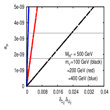
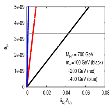
Figure 2: The muon $g-2$ as a function of the product $\delta_{\Sigma_{2}}\cdot\delta_{U_{2}}$, for $m_{\nu^{\prime}}=100,~{}200,~{}400$ GeV, $m_{\tau^{\prime}}=m_{\nu^{\prime}}$ and with $m_{H^{+}}=500$ GeV (left) and $m_{H^{+}}=700$ GeV (right). The horizontal lines are the measured 1-$\sigma$ bounds on $a_{\mu}$ (see Eq. 4).

In what follows we will consider the constraints from the lepton flavor violating decays $\ell_{i}\to\ell_{j}\gamma$ and from the decay $B_{s}\to\mu^{+}\mu^{-}$, both of which are sensitive to the quantities $\delta_{U_{2}}$ and $\delta_{\Sigma_{2}}$, as will be explained below.

III Constraints from Lepton flavour violation

LFV decays such as $\tau\to\mu\gamma$ and $\mu\to e\gamma$, which are absent in the SM, are often found useful for constraining NP models that can potentially contribute to the $\mu$AMM, as such processes do not suffer from hadronic uncertainties. The current experimental 90%CL upper bounds on these LFV decays are pdg ; meg

$$Br(\tau\to\mu\gamma)<4.4\times 10^{-8}~{}~{},~{}~{}Br(\mu\to e\gamma)<2.4\times 10^{-12}~{}.$$ (23)

Let us define the amplitude for the transition $\ell_{i}\to\ell_{j}\gamma$ as

$${\cal M}(\ell_{i}\to\ell_{j}\gamma)=\bar{u}_{\ell_{j}}(p^{\prime})\left[i\sigma_{\mu\nu}q^{\nu}\left(A+B\gamma_{5}\right)\right]u_{\ell_{i}}(p)\epsilon^{\mu\ast}\,,$$ (24)

where $\epsilon^{\mu\ast}$ is the photon polarization. The decay width is then given by

$$\Gamma(\ell_{i}\to\ell_{j}\gamma)=\frac{m^{3}_{\ell_{i}}}{8\pi}\left(1-\frac{m_{\ell_{j}}^{2}}{m_{\ell_{i}}^{2}}\right)\left[\left(1+\frac{m_{\ell_{j}}^{2}}{m_{\ell_{i}}^{2}}\right)\left(|A|^{2}+|B|^{2}\right)+4\frac{m_{\ell_{j}}}{m_{\ell_{i}}}\left(|A|^{2}-|B|^{2}\right)\right]~{}.$$ (25)

Here again, the new 4G2HDM amplitude ${\cal M}(\ell_{i}\to\ell_{j}\gamma)^{4G2HDM}$ can be divided as

$${\cal M}(\ell_{i}\to\ell_{j}\gamma)^{4G2HDM}\equiv{\cal M}^{SM4}_{W}(\ell_{i}\to\ell_{j}\gamma)+{\cal M}^{4G2HDM}_{H^{+}}(\ell_{i}\to\ell_{j}\gamma)+{\cal M}^{4G2HDM}_{{\cal H}^{0}}(\ell_{i}\to\ell_{j}\gamma)~{},$$ (26)

where ${\cal M}^{SM4}_{W}(\ell_{i}\to\ell_{j}\gamma)$ are the SM4-like W-exchange contribution which is obtained from the diagram (right) of Fig. 1 with $\phi^{\pm}$ replaced by $W^{\pm}$ plus the diagrams which contain the self-energy corrections to the external fermion line $\ell_{i}$ or $\ell_{j}$. In particular, using the definition in Eq. 24 and taking the limit $m_{\ell_{j}}\to 0$, the net contribution to ${\cal M}^{SM4}_{W}(\ell_{i}\to\ell_{j}\gamma)$ with internal $\nu^{\prime}$ in the loop is given by beneke_buras

$$A^{SM4}_{W}=B^{SM4}_{W}=\frac{eG_{F}m_{\ell_{i}}}{4\sqrt{2}\pi^{2}}U_{j4}U^{\ast}_{i4}F(x_{\nu^{\prime}})~{},$$ (27)

where $x_{i}=m^{2}_{i}/M^{2}_{W}$ and $F(x_{i})$ is given by

$$F(x_{i})=\frac{x_{i}(1-6x_{i}+3x^{2}_{i}+2x^{3}_{i}-6x^{2}_{i}\log{x_{i}})}{4(1-x_{i})^{4}}~{}.$$ (28)

Here also, we find that ${\cal M}^{SM4}_{W}(\ell_{i}\to\ell_{j}\gamma)$ is much smaller than the charged and neutral Higgs amplitudes, ${\cal M}^{4G2HDM}_{H^{+}}(\ell_{i}\to\ell_{j}\gamma)$ and ${\cal M}^{4G2HDM}_{{\cal H}^{0}}(\ell_{i}\to\ell_{j}\gamma)$ (calculated from the diagrams in Fig. 1), for which we obtain

$$A_{H^{-}}^{4G2HDM} = \frac{e}{32\pi^{2}}\left\{(m_{\ell_{i}}+m_{\ell_{j}})\left({S^{H^{-}}_{\ell_{i}\nu^{\prime}}}^{\ast}S^{H^{-}}_{\ell_{j}\nu^{\prime}}+{P^{H^{-}}_{\ell_{i}\nu^{\prime}}}^{\ast}P^{H^{-}}_{\ell_{j}\nu^{\prime}}\right)I_{1}^{H^{+}}+2m_{\nu^{\prime}}\left({S^{H^{-}}_{\ell_{i}\nu^{\prime}}}^{\ast}S^{H^{-}}_{\ell_{j}\nu^{\prime}}-{P^{H^{-}}_{\ell_{i}\nu^{\prime}}}^{\ast}P^{H^{-}}_{\ell_{j}\nu^{\prime}}\right)I_{2}^{H^{+}}\right\}~{},$$ (29)

$$B_{H^{-}}^{4G2HDM} = \frac{e}{32\pi^{2}}\left\{(m_{\ell_{i}}-m_{\ell_{j}})\left({S^{H^{-}}_{\ell_{i}\nu^{\prime}}}^{\ast}P^{H^{-}}_{\ell_{j}\nu^{\prime}}+S^{H^{-}}_{\ell_{j}\nu^{\prime}}{P^{H^{-}}_{\ell_{i}\nu^{\prime}}}^{\ast}\right)I_{1}^{H^{+}}+2m_{\nu^{\prime}}\left({S^{H^{-}}_{\ell_{i}\nu^{\prime}}}^{\ast}P^{H^{-}}_{\ell_{j}\nu^{\prime}}-S^{H^{-}}_{\ell_{j}\nu^{\prime}}{P^{H^{-}}_{\ell_{i}\nu^{\prime}}}^{\ast}\right)I_{2}^{H^{+}}\right\}~{},$$ (30)

$$A_{{\cal H}^{0}}^{4G2HDM} = \frac{e}{32\pi^{2}}\left\{(m_{\ell_{i}}+m_{\ell_{j}})\left({S^{{\cal H}^{0}}_{\ell_{i}\tau^{\prime}}}^{\ast}S^{{\cal H}^{0}}_{\ell_{j}\tau^{\prime}}+{P^{{\cal H}^{0}}_{\ell_{i}\tau^{\prime}}}^{\ast}P^{{\cal H}^{0}}_{\ell_{j}\tau^{\prime}}\right)I_{1}^{{\cal H}^{0}}+2m_{\tau^{\prime}}\left({S^{{\cal H}^{0}}_{\ell_{i}\tau^{\prime}}}^{\ast}S^{{\cal H}^{0}}_{\ell_{j}\tau^{\prime}}-{P^{{\cal H}^{0}}_{\ell_{i}\tau^{\prime}}}^{\ast}P^{{\cal H}^{0}}_{\ell_{j}\tau^{\prime}}\right)I_{2}^{{\cal H}^{0}}\right\}~{},$$ (31)

$$B_{{\cal H}^{0}}^{4G2HDM} = \frac{e}{32\pi^{2}}\left\{(m_{\ell_{i}}-m_{\ell_{j}})\left({S^{{\cal H}^{0}}_{\ell_{i}\tau^{\prime}}}^{\ast}P^{{\cal H}^{0}}_{\ell_{j}\tau^{\prime}}+S^{{\cal H}^{0}}_{\ell_{j}\tau^{\prime}}{P^{{\cal H}^{0}}_{\ell_{i}\tau^{\prime}}}^{\ast}\right)I_{1}^{{\cal H}^{0}}+2m_{\tau^{\prime}}\left({S^{{\cal H}^{0}}_{\ell_{i}\tau^{\prime}}}^{\ast}P^{{\cal H}^{0}}_{\ell_{j}\tau^{\prime}}-S^{{\cal H}^{0}}_{\ell_{j}\tau^{\prime}}{P^{{\cal H}^{0}}_{\ell_{i}\tau^{\prime}}}^{\ast}\right)I_{2}^{{\cal H}^{0}}\right\}~{},$$ (32)

where the loop integrals $I_{1}^{H^{+}}$, $I_{2}^{H^{+}}$, $I_{1}^{{\cal H}^{0}}$ and $I_{2}^{{\cal H}^{0}}$ are given by (taking $m_{\ell_{i}}^{2},m_{\ell_{j}}^{2}\ll m_{\cal H}^{2},m_{\nu^{\prime}}^{2},m_{\tau^{\prime}}^{2}$):

$$I_{1}^{H^{+}} \approx \int^{1}_{0}dx\frac{x^{2}(x-1)}{m^{2}_{H^{-}}\,x+m^{2}_{\nu^{\prime}}(1-x)}~{},$$

$$I_{2}^{H^{+}} \approx \int^{1}_{0}dx\frac{x(x-1)}{m^{2}_{H^{-}}\,x+m^{2}_{\nu^{\prime}}(1-x)}~{},$$

$$I_{1}^{{\cal H}^{0}} \approx \int^{1}_{0}dx\frac{x^{2}(1-x)}{m^{2}_{\tau^{\prime}}\,x+m^{2}_{{\cal H}^{0}}(1-x)}~{},$$

$$I_{2}^{{\cal H}^{0}} \approx \int^{1}_{0}dx\frac{x^{2}}{m^{2}_{\tau^{\prime}}\,x+m^{2}_{{\cal H}^{0}}(1-x)}~{}.$$

The dominant terms in Eqs. 29-32 are the ones proportional to $m_{\nu^{\prime}}$ from the charged Higgs exchange contribution,

$$\left({S^{H^{-}}_{\ell_{i}\nu^{\prime}}}^{\ast}S^{H^{-}}_{\ell_{j}\nu^{\prime}}-{P^{H^{-}}_{\ell_{i}\nu^{\prime}}}^{\ast}P^{H^{-}}_{\ell_{j}\nu^{\prime}}\right) = -\frac{g^{2}}{4}\frac{m_{\nu^{\prime}}m_{\tau^{\prime}}}{m_{W}^{2}}f_{\beta}^{2}|U_{44}|^{2}|\Sigma_{44}^{\nu}|^{2}\left(1-\frac{t_{\beta}}{f_{\beta}\Sigma_{44}^{\nu}}\right)\left(\delta_{U_{i}}^{\ast}\delta_{\Sigma_{j}}+\delta_{U_{j}}\delta_{\Sigma_{i}}^{\ast}\right)~{},$$

$$\left({S^{H^{-}}_{\ell_{i}\nu^{\prime}}}^{\ast}P^{H^{-}}_{\ell_{j}\nu^{\prime}}-{S^{H^{-}}_{\ell_{i}\nu^{\prime}}}^{\ast}P^{H^{-}}_{\ell_{j}\nu^{\prime}}\right) = -\frac{g^{2}}{4}\frac{m_{\nu^{\prime}}m_{\tau^{\prime}}}{m_{W}^{2}}f_{\beta}^{2}|U_{44}|^{2}|\Sigma_{44}^{\nu}|^{2}\left(1-\frac{t_{\beta}}{f_{\beta}\Sigma_{44}^{\nu}}\right)\left(\delta_{U_{i}}^{\ast}\delta_{\Sigma_{j}}-\delta_{U_{j}}\delta_{\Sigma_{i}}^{\ast}\right)~{},$$ (34)

since the terms proportional to $m_{\tau^{\prime}}$ in the neutral Higgs exchanges vanish due to $|S^{{\cal H}^{0}}_{\ell_{i}\tau^{\prime}}|=|P^{{\cal H}^{0}}_{\ell_{i}\tau^{\prime}}|$ (see Eq. 18).

We thus find that in our 4G2HDM, the decays $\mu\to e\gamma$ and $\tau\to\mu\gamma$ are sensitive to $\delta_{U_{2}}$ and $\delta_{\Sigma_{2}}$ through the products $(\delta_{U_{2}}\delta_{\Sigma_{1}},\delta_{U_{1}}\delta_{\Sigma_{2}})$ and $(\delta_{U_{3}}\delta_{\Sigma_{2}},\delta_{U_{2}}\delta_{\Sigma_{3}})$, respectively, so that, in principle, one can avoid constraints on the quantities $\delta_{U_{2}}$ and $\delta_{\Sigma_{2}}$ if $\delta_{U_{1}},\delta_{U_{3}},\delta_{\Sigma_{1}}$ and $\delta_{\Sigma_{3}}$ are sufficiently small.

In Figs. 3 we plot $BR(\mu\to e\gamma)$ as a function of $\delta_{U_{1}}\cdot\delta_{\Sigma_{2}}$ and $\delta_{U_{2}}\cdot\delta_{\Sigma_{1}}$, for $m_{\nu^{\prime}}=100,~{}200,~{}400$ GeV, $m_{H^{+}}=500$ GeV and fixing $m_{\tau^{\prime}}=m_{\nu^{\prime}}$. We see that for e.g. $m_{\nu^{\prime}}=100$ GeV and for values of $\delta_{U_{2}}$ and $\delta_{\Sigma_{2}}$ of ${\cal O}(0.1)$ [for which the product $\delta_{U_{2}}\cdot\delta_{\Sigma_{2}}$ reproduces the measured $a_{\mu}$ (see Fig. 2)], $\delta_{U_{1}}$ and $\delta_{\Sigma_{1}}$ are required to be smaller than ${\rm few}\times 10^{-5}$, implying that $\delta_{U_{1}}\ll\delta_{U_{2}}$ and $\delta_{\Sigma_{1}}\ll\delta_{\Sigma_{2}}$.

In Fig. 4 we plot $BR(\tau\to\mu\gamma)$ as a function of $\delta_{U_{2}}\cdot\delta_{\Sigma_{3}}$ and $\delta_{U_{3}}\cdot\delta_{\Sigma_{2}}$, and in Fig. 5 we give a scatter plot of the allowed values in the $\delta_{\Sigma_{3}}-\delta_{U_{3}}$ plane, for which $BR(\tau\to\mu\gamma)<4.4\times 10^{-8}$ (i.e., below its 90%CL bound). In both plots we use $m_{\nu^{\prime}}=100,~{}200,~{}400$ GeV, $m_{H^{+}}=500$ GeV and we fix $m_{\tau^{\prime}}=m_{\nu^{\prime}}$. The individual couplings $\delta_{U_{2}}$ and $\delta_{\Sigma_{2}}$ are randomly chosen to always be within values that reproduce the measured $a_{\mu}$ (see Fig. 2). We see that the products $\delta_{U_{2}}\cdot\delta_{\Sigma_{3}}$ and $\delta_{U_{3}}\cdot\delta_{\Sigma_{2}}$ are required to be at most ${\rm few}\times 0.001$, in order to be consistent with the current bounds on $BR(\tau\to\mu\gamma)$.

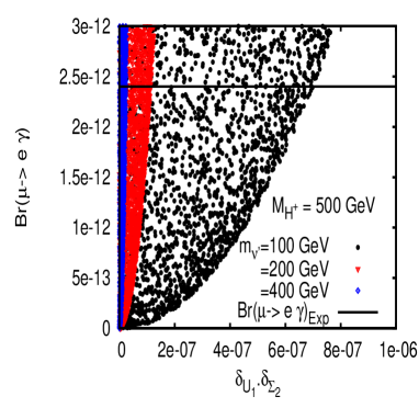
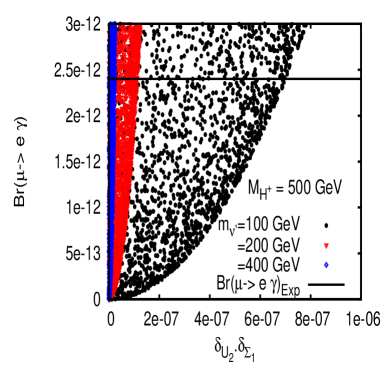
Figure 3: $BR(\mu\to e\gamma)$ as a function of $\delta_{U_{1}}\cdot\delta_{\Sigma_{2}}$ (left) and of $\delta_{U_{2}}\cdot\delta_{\Sigma_{1}}$ (right), for $m_{\nu^{\prime}}=100,~{}200,~{}400$ GeV, $m_{\tau^{\prime}}=m_{\nu^{\prime}}$ and with $m_{H^{+}}=500$ GeV. Also shown (horizontal line) is the $90\%CL$ upper limit on $BR(\mu\to e\gamma)$ (see Eq. 23).

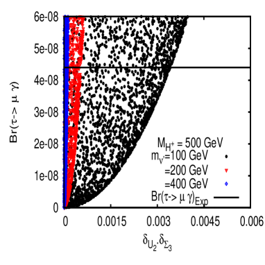
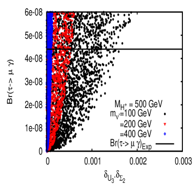
Figure 4: $BR(\tau\to\mu\gamma)$ as a function of $\delta_{U_{3}}\cdot\delta_{\Sigma_{2}}$ (left) and $\delta_{U_{2}}\cdot\delta_{\Sigma_{3}}$ (right), for $m_{\nu^{\prime}}=100,~{}200,~{}400$ GeV, $m_{\tau^{\prime}}=m_{\nu^{\prime}}$ and with $m_{H^{+}}=500$ GeV. Also shown (horizontal line) is the $90\%CL$ upper limit on $BR(\tau\to\mu\gamma)$ (see Eq. 23).

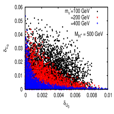
Figure 5: Allowed values in the $\delta_{\Sigma_{3}}-\delta_{U_{3}}$ plane, for which $BR(\tau\to\mu\gamma)<4.4\times 10^{-8}$ (i.e., below its 90%CL bound), for $m_{\nu^{\prime}}=100,~{}200,~{}400$ GeV, $m_{\tau^{\prime}}=m_{\nu^{\prime}}$ and with $m_{H^{+}}=500$ GeV. The couplings $\delta_{U_{2}}$ and $\delta_{\Sigma_{2}}$ are chosen randomly in the range $[0,0.2]$ so that the product $\delta_{U_{2}}\cdot\delta_{\Sigma_{2}}$ reproduces the measured $a_{\mu}$ (see Fig. 2).

We can thus identify a typical benchmark texture for the 4th generation elements of the CKM-like PMNS matrix, $U_{i4}$, and for the new mixing matrix $\Sigma^{e}_{4i}$ that can explain the observed $\mu$AMM and still be consistent with the current LFV constraints

$$U_{i4}\sim(\Sigma^{e}_{4i})^{T}\simeq\left(\begin{array}[]{c}\epsilon^{5}\\ \epsilon\\ \epsilon^{2}\\ 1\end{array}\right)~{},$$ (39)

where e.g., $\epsilon\sim 0.1$ for $m_{\nu^{\prime}}=100$ GeV.

Admittedly, the above texture implies a hierarchical pattern which is different from the observed hierarchy in the quark’s CKM matrix - usually termed as “normal”. Nonetheless, without a fundamental theory of flavor, our insights for flavor should be data driven also in the leptonic sector. Besides, the above texture is sensitive to the current precision in the measurement of the muon g-2 which can change e.g., if more accurate calculations end up showing that part of the hadronic contributions cannot be ignored.

In Table 1 we list several representative values of the couplings $\delta_{U_{2}}$, $\delta_{\Sigma_{2}}$ and the products $(\delta_{U_{1}},\delta_{\Sigma_{2}})$, $(\delta_{U_{2}},\delta_{\Sigma_{1}})$, $(\delta_{U_{3}},\delta_{\Sigma_{2}})$ and $(\delta_{U_{2}},\delta_{\Sigma_{3}})$ that are consistent with the measured $\mu$AMM (i.e., $a_{\mu}^{exp}$ given in eq. 4), and that give LFV branching fractions Br$(\tau\to\mu\gamma)$ and Br$(\mu\to e\gamma)$ at the level of ${\cal O}(10^{-13})$ and ${\cal O}(10^{-9})$, respectively, that are accessible to near future experiments meg ; superb .

$m_{\nu^{\prime}}$	$\delta_{U_{2}}=\delta_{\Sigma_{2}}$	$a_{\mu}$	Br$(\mu\to e\gamma)$	$\delta_{U_{1}}.\delta_{\Sigma_{2}}$	$\delta_{U_{2}}.\delta_{\Sigma_{1}}$	Br$(\tau\to\mu\gamma)$	$\delta_{U_{3}}.\delta_{\Sigma_{2}}$	$\delta_{U_{2}}.\delta_{\Sigma_{3}}$
(GeV)		$\times 10^{9}$	$\times 10^{12}$	$\times 10^{7}$	$\times 10^{7}$	$\times 10^{8}$	$\times 10^{4}$	$\times 10^{4}$
			1.20	1.31	4.57	1.78	1.85	20.40
100	0.12	2.07	0.64	2.45	2.25	0.77	3.21	5.90
			0.14	1.51	0.45	0.26	2.00	2.12
			1.21	0.22	0.76	2.03	0.51	3.65
200	0.05	2.25	0.62	0.51	0.25	0.79	0.41	2.25
			0.11	0.43	0.61	0.18	0.16	1.07
			1.39	0.16	0.04	2.14	0.73	0.12
400	0.022	2.19	0.69	0.07	0.10	0.78	0.40	0.21
			0.17	0.05	0.02	0.13	0.11	0.14

Table 1: The calculated $a_{\mu}$ and the branching fractions for the LFV decays $\tau\to\mu\gamma$ and $\mu\to e\gamma$ in the 4G2HDM, for several representative values of the couplings $\delta_{U_{2}}$, $\delta_{\Sigma_{2}}$ and the products $(\delta_{U_{1}},\delta_{\Sigma_{2}})$, $(\delta_{U_{2}},\delta_{\Sigma_{1}})$, $(\delta_{U_{3}},\delta_{\Sigma_{2}})$ and $(\delta_{U_{2}},\delta_{\Sigma_{3}})$ that are consistent with the measured $\mu$AMM and which give Br$(\tau\to\mu\gamma)$ and Br$(\mu\to e\gamma)$ at the level of ${\cal O}(10^{-13})$ and ${\cal O}(10^{-9})$, respectively.

IV Constraints from $B_{s}\to\ell^{+}\ell^{-}$

In the SM, tree level $b\to s$ FCNC transitions are forbidden, and also the purely leptonic $B_{s}\to\ell^{+}\ell^{-}$ decays, with $\ell=e,~{}\mu,~{}\tau$, suffer from chiral suppression and are therefore very sensitive to new physics. The SM predicted branching fractions for these decays are appreciably smaller than those of the semi-leptonic decays. For example, for $B_{s}\to\mu^{+}\mu^{-}$, the SM prediction is ajb10B

$$Br(B_{s}\to\mu^{+}\mu^{-})=(3.2\pm 0.2)\cdot 10^{-9}~{}.$$ (40)

In the LHC era the current limit on $Br(B_{s}\to\mu^{+}\mu^{-})$ has been improved. A combined analysis by LHCb and CMS, using 0.34$fb^{-1}$ and 1.14$fb^{-1}$ data sample, respectively, yields lhcb1

$$Br(B_{s}\to\mu^{+}\mu^{-})<1.08\times 10^{-8}\;,\hskip 30.0pt(LHCb+CMS)@95\%CL$$ (41)

whereas the same measurement by CDF-II, using a 7$fb^{-1}$ data sample, gives cdfII

$$Br(B_{s}\to\mu^{+}\mu^{-})<4.0\times 10^{-8}\hskip 35.0ptCDF@95\%CL.$$ (42)

In fact, LHCb has the sensitivity to measure the $Br(B_{s}\to\mu^{+}\mu^{-})$ down to $\sim 2\times 10^{-9}$, which is about $5\sigma$ smaller than the SM prediction.

Figure 6: Dominant SM diagrams in the $B_{d^{\prime}}\to\ell^{+}\ell^{-}$ decay.

In general, the matrix element for the decay ${\bar{B}_{s}}\to\ell^{+}\ell^{-}$ can be written as mBs

$${\cal M}=\frac{G_{F}\alpha}{2\sqrt{2}\pi\sin\theta_{W}^{2}}\left[F_{S}\,{\bar{\ell}}\ell+F_{P}\,{\bar{\ell}}\gamma_{5}\ell+F_{A}\,P^{\mu}{\bar{\ell}}\gamma_{\mu}\gamma_{5}\ell\right],\,$$ (43)

where $P^{\mu}$ is the four momentum of the initial $B_{s}$ meson and $F_{i}$’s are functions of Lorentz invariant quantities. Squaring the matrix and summing over the lepton spins, we obtain the branching fraction

$$Br({\bar{B}_{s}}\to\ell^{+}\ell^{-})=\frac{G_{F}^{2}\alpha^{2}M_{B_{s}}\tau_{B_{s}}}{64\pi^{3}}\sqrt{1-\frac{4m_{\ell}^{2}}{M_{B_{s}}^{2}}}\left[\left(1-\frac{4m_{\ell}^{2}}{M_{B_{s}}^{2}}\right)|F_{S}|^{2}+|F_{P}+2m_{\ell}F_{A}|^{2}\right].$$ (44)

In the SM, the dominant effect in ${\bar{B}_{s}}\to\ell^{+}\ell^{-}$ arise from the diagrams shown in Fig. 6, which contribute to $F_{A}$ in Eq. 43. At next-to-leading (NLO) QCD corrections, the net contribution in $F_{A}$ is given by Buchalla:1993bv ; Misiak:1999yg

$$F_{A}^{SM}=-\,i\,f_{B_{s}}\,V_{tb}V_{ts}^{\ast}\,Y(x_{t})=-\,i\,f_{B_{s}}\,V_{tb}V_{ts}^{\ast}\times 0.997\left[\frac{m_{t}(m_{t})}{166{\rm GeV}}\right]^{1.55}.$$ (45)

In the SM4 it is again $F_{A}$ which receives a non-zero contribution:

$$F_{A}^{SM4}=(F_{A}^{SM4})^{peng}+(F_{A}^{SM4})^{box},$$ (46)

where $(F_{A}^{SM4})^{peng}$ is the contributions from the Z-penguin diagrams in Fig. 6 with the top quark replaced by a $t^{\prime}$, and $(F_{A}^{SM4})^{box}$ is the contribution from the box diagram in Fig. 6 with the replacement $t\to t^{\prime}$ and $\nu_{\ell}\to\nu^{\prime}$. At leading-order (LO) in QCD, they are given by

$$(F_{A}^{SM4})^{peng}=-\,i\,f_{B_{s}}V_{t^{\prime}b}V_{t^{\prime}s}^{\ast}\frac{x_{t^{\prime}}}{8}\left[\frac{6-x_{t^{\prime}}}{1-x_{t^{\prime}}}+\frac{3x_{t^{\prime}}+2}{(1-x_{t^{\prime}})^{2}}\ln{x_{t^{\prime}}}\right],$$ (47)

$$(F_{A}^{SM4})^{box}=-\,i\,f_{B_{s}}\,V_{t^{\prime}b}V_{t^{\prime}s}^{\ast}\,|U_{24}|^{2}\frac{B_{0}(x_{t^{\prime}},x_{\nu^{\prime}})}{4},$$ (48)

with

$$B_{0}(x_{i},x_{j}) = x_{i}\,x_{j}\left[-\frac{3}{4}\frac{1}{(1-x_{i})(1-x_{j})}+\frac{\ln{x_{i}}}{(x_{i}-x_{j})(1-x_{i})^{2}}\left(1-2x_{i}+\frac{x_{i}^{2}}{4}\right)\right.$$ (49)

$$\hskip 15.0pt\left.+\frac{\ln{x_{j}}}{(x_{j}-x_{i})(1-x_{j})^{2}}\left(1-2x_{j}+\frac{x_{j}^{2}}{4}\right)\right].$$

In our 4G2HDM, we have additional contributions to $F_{A}$ coming from the charged Higgs exchange penguin and box diagrams (replacing $W^{+}\to H^{+}$ in Fig. 6) and, in addition, there are new contributions to $F_{S}$ and $F_{P}$. For our purpose, we are interested only in the diagrams that are sensitive to the $\ell^{\pm}\nu^{\prime}H^{\pm}$ vertex, which are, therefore, directly related to the muon g-2. The dominant diagrams that contribute to the ${\bar{B}_{s}}\to\ell^{+}\ell^{-}$ decay with this vertex are the Higgs-exchange box diagrams in Fig. 6, where one or two $W$-bosons are replaced by $H^{+}$ and $(t,\nu_{\ell})$ are being replaced by both $(t,\nu^{\prime})$ and $(t^{\prime},\nu^{\prime})$. Thus, the net contributions to $F_{S}$, $F_{P}$ and $F_{A}$ in Eq. 43 can be written as

$$F_{S}=F_{S}^{H},\hskip 10.0ptF_{P}=F_{P}^{H}\hskip 10.0ptand\hskip 10.0ptF_{A}=F_{A}^{SM}+F_{A}^{SM4}+F_{A}^{H}~{},$$ (50)

where $F_{S}^{H},~{}F_{P}^{H}$ and $F_{A}^{H}$ are the contributions from the dominant new Higgs-exchange box diagrams, which, for the $(t^{\prime},\nu^{\prime})$ exchange, are given by

$$F_{S}^{H} = (F_{S})_{HH}^{box}+(F_{S})_{WH}^{box},$$ (51)

$$= -\frac{i\,2f_{B_{s}}}{g^{2}}\,\frac{M_{B_{s}}^{2}}{m_{b}+m_{s}}\left[\frac{m_{\nu^{\prime}}m_{t^{\prime}}}{M_{H^{-}}^{4}}\left({S_{t^{\prime}s}^{{H^{-}}}}^{\ast}P_{t^{\prime}b}^{H^{-}}-S_{t^{\prime}b}^{H^{-}}{P_{t^{\prime}s}^{{H^{-}}}}^{\ast}\right)\left(\left|S^{H^{-}}_{\mu\nu^{\prime}}\right|^{2}-\left|P^{H^{-}}_{\mu\nu^{\prime}}\right|^{2}\right)B_{HH}^{S}(y_{t^{\prime}},y_{\nu^{\prime}})\right.$$

$$\hskip 76.82234pt+\frac{g}{2\sqrt{2}m_{W}}\left\{V_{t^{\prime}b}U_{24}^{\ast}\left({S_{t^{\prime}s}^{H^{-}}}^{\ast}+{P_{t^{\prime}s}^{\cal H}}^{\ast}\right)\left({S_{\mu\nu^{\prime}}^{H^{-}}}+{P_{\mu\nu^{\prime}}^{H^{-}}}\right)-V_{t^{\prime}s}^{\ast}U_{24}\left({S_{t^{\prime}b}^{H^{-}}}+{P_{t^{\prime}b}^{H^{-}}}\right)\right.$$

$$\hskip 76.82234pt\left.\left.\left({S_{\mu\nu^{\prime}}^{H^{-}}}^{\ast}+{P_{\mu\nu^{\prime}}^{H^{-}}}^{\ast}\right)\right\}B_{WH}^{S}(x_{t^{\prime}},x_{\nu^{\prime}},x_{H})\right]$$

$$F_{P}^{H} = (F_{P})_{HH}^{box}+(F_{P})_{WH}^{box},$$ (52)

$$= -\frac{i\,2f_{B_{s}}}{g^{2}}\,\frac{M_{B_{s}}^{2}}{m_{b}+m_{s}}\left[\frac{m_{\nu^{\prime}}m_{t^{\prime}}}{M_{H^{-}}^{4}}\left({S_{t^{\prime}s}^{H^{-}}}^{\ast}P_{t^{\prime}b}^{H^{-}}-S_{t^{\prime}b}^{H^{-}}{P_{t^{\prime}s}^{H^{-}}}^{\ast}\right)\left(P_{\mu\nu^{\prime}}^{H^{-}}{S_{\mu\nu^{\prime}}^{H^{-}}}^{\ast}-S_{\mu\nu^{\prime}}^{H^{-}}{P_{\mu\nu^{\prime}}^{H^{-}}}^{\ast}\right)B_{HH}^{P}(y_{t^{\prime}},y_{\nu^{\prime}})\right.$$

$$\hskip 76.82234pt+\frac{g}{2\sqrt{2}m_{W}}\left\{V_{t^{\prime}b}U_{24}^{\ast}\left({S_{t^{\prime}s}^{H^{-}}}^{\ast}+{P_{t^{\prime}s}^{H^{-}}}^{\ast}\right)\left({S_{\mu\nu^{\prime}}^{H^{-}}}+{P_{\mu\nu^{\prime}}^{H^{-}}}\right)+V_{t^{\prime}s}^{\ast}U_{24}\left({S_{t^{\prime}b}^{H^{-}}}+{P_{t^{\prime}b}^{H^{-}}}\right)\right.$$

$$\hskip 76.82234pt\left.\left.\left({S_{\mu\nu^{\prime}}^{H^{-}}}^{\ast}+{P_{\mu\nu^{\prime}}^{H^{-}}}^{\ast}\right)\right\}B_{WH}^{P}(x_{t^{\prime}},x_{\nu^{\prime}},x_{H})\right]$$

$$F_{A}^{H} = (F_{A})_{HH}^{box}+(F_{A})_{WH}^{box},$$ (53)

$$= -\frac{i\,2f_{B_{s}}}{g^{2}}\,\left[\frac{1}{4\,M_{H^{-}}^{2}}\left(S_{t^{\prime}s}^{H^{-}}{P_{t^{\prime}b}^{H^{-}}}^{\ast}+{S_{t^{\prime}b}^{H^{-}}}^{\ast}P_{t^{\prime}s}^{H^{-}}\right)\left(P_{\mu\nu^{\prime}}^{H^{-}}{S_{\mu\nu^{\prime}}^{H^{-}}}^{\ast}+S_{\mu\nu^{\prime}}^{H^{-}}{P_{\mu\nu^{\prime}}^{H^{-}}}^{\ast}\right)B_{HH}^{A}(y_{t^{\prime}},y_{\nu^{\prime}})\right.$$

$$\hskip 34.14322pt+\frac{g}{2\sqrt{2}m_{W}}\frac{m_{\nu^{\prime}}m_{t^{\prime}}}{m_{W}^{2}}\left\{V_{t^{\prime}b}U_{24}^{\ast}\left({P_{t^{\prime}s}^{H^{-}}}^{\ast}-{S_{t^{\prime}s}^{H^{-}}}^{\ast}\right)\left({S_{\mu\nu^{\prime}}^{H^{-}}}-{P_{\mu\nu^{\prime}}^{H^{-}}}\right)+V_{t^{\prime}s}^{\ast}U_{24}\left({P_{t^{\prime}b}^{H^{-}}}-{S_{t^{\prime}b}^{H^{-}}}\right)\right.$$

$$\hskip 34.14322pt\left.\left.\left({S_{\mu\nu^{\prime}}^{H^{-}}}^{\ast}-{P_{\mu\nu^{\prime}}^{H^{-}}}^{\ast}\right)\right\}B_{WH}^{A}(x_{t^{\prime}},x_{\nu^{\prime}},x_{H})\right],$$

where $y_{i}=m_{i}^{2}/M_{H^{-}}^{2}$, $x_{i}=m_{i}^{2}/M_{W}^{2}$ and the loop-functions are given by

$$B_{HH}^{S}(y_{i},y_{j}) = B_{HH}^{P}(y_{i},y_{j})=\frac{1}{y_{i}-y_{j}}\left\{\frac{y_{j}\ln{y_{j}}}{(1-y_{j})^{2}}-\frac{y_{i}\ln{y_{i}}}{(1-y_{i})^{2}}\right\}-\frac{1}{(1-y_{i})(1-y_{j})}$$

$$B_{WH}^{S}(x_{i},x_{j},x_{H}) = B_{WH}^{P}(x_{i},x_{j},x_{H})=\frac{x_{H}^{2}\ln{x_{H}}}{(x_{H}-1)(x_{H}-x_{i})(x_{H}-x_{j})}$$

$$+\frac{x_{i}^{2}\ln{x_{i}}}{(x_{i}-1)(x_{i}-x_{H})(x_{i}-x_{j})}+\frac{x_{j}^{2}\ln{x_{j}}}{(x_{j}-1)(x_{j}-x_{H})(x_{j}-x_{i})}$$

$$B_{HH}^{A}(y_{i},y_{j}) = \frac{y_{j}^{2}\ln{y_{j}}}{(1-y_{j})^{2}\,(y_{j}-y_{i})}+\frac{y_{i}^{2}\ln{y_{i}}}{(1-y_{i})^{2}\,(y_{i}-y_{j})}+\frac{1}{(1-y_{i})(1-y_{j})}$$

$$B_{WH}^{A}(x_{i},x_{j},x_{H}) = \frac{\,x_{H}\ln{x_{H}}}{(x_{H}-1)(x_{H}-x_{i})(x_{H}-x_{j})}+\frac{x_{i}\ln{x_{i}}}{(x_{i}-1)(x_{i}-x_{H})(x_{i}-x_{j})}$$ (54)

$$+\frac{x_{j}\ln{x_{j}}}{(x_{j}-1)(x_{j}-x_{H})(x_{j}-x_{i})}~{}.$$

Also, $S_{\mu\nu^{\prime}}^{H^{-}}$, $P_{\mu\nu^{\prime}}^{H^{-}}$ are defined in Eq. 18 and

$$S_{t^{\prime}b}^{H^{-}} = (m_{b}-m_{t^{\prime}})t_{\beta}V_{t^{\prime}b}+f_{\beta}V_{t^{\prime}b}\left[\left(m_{t^{\prime}}\Sigma_{44}^{u*}-m_{b}\Sigma_{33}^{d}\right)+\left(m_{t}\Sigma_{34}^{u*}\frac{V_{tb}}{V_{t^{\prime}b}}-m_{b^{\prime}}\Sigma_{43}^{d}\frac{V_{t^{\prime}b^{\prime}}}{V_{t^{\prime}b}}\right)\right],$$

$$P_{t^{\prime}b}^{H^{-}} = (m_{b}+m_{t^{\prime}})t_{\beta}V_{t^{\prime}b}-f_{\beta}V_{t^{\prime}b}\left[\left(m_{t^{\prime}}\Sigma_{44}^{u*}+m_{b}\Sigma_{33}^{d}\right)+\left(m_{t}\Sigma_{34}^{u*}\frac{V_{tb}}{V_{t^{\prime}b}}+m_{b^{\prime}}\Sigma_{43}^{d}\frac{V_{t^{\prime}b^{\prime}}}{V_{t^{\prime}b}}\right)\right],$$

$$S_{t^{\prime}s}^{H^{-}} = -P_{t^{\prime}s}^{H^{-}}=-m_{t^{\prime}}t_{\beta}V_{t^{\prime}s}+f_{\beta}\left(m_{t^{\prime}}V_{t^{\prime}s}\Sigma_{44}^{u*}+m_{t}V_{ts}\Sigma_{34}^{u*}\right)~{}.$$ (55)

For the couplings $S_{t^{\prime}b}^{H^{-}},~{}S_{t^{\prime}s}^{H^{-}},~{}P_{t^{\prime}b}^{H^{-}},~{}P_{t^{\prime}s}^{H^{-}}$ we use the 4G2HDM Yukawa terms in the quark sector as given in 4G2HDM , where $\Sigma^{u}$ and $\Sigma^{d}$ are the corresponding new mixing matrices in the up and down-quark sectors, respectively, obtained after diagonalizing the quarks mass matrices. In particular, adopting the type I 4G2HDM of 4G2HDM , these matrices are given by

$$\Sigma_{ij}^{d}=D_{R,4i}^{\star}D_{R,4j}~{},~{}\Sigma_{ij}^{u}=U_{R,4i}^{\star}U_{R,4j}~{},$$ (56)

in analogy with Eq. 16, where $D_{R},U_{R}$ are the rotation (unitary) matrices of the right-handed down and up-quarks, respectively. They can be approximated by (see 4G2HDM )

$$\Sigma^{d}\simeq\left(\begin{array}[]{cccc}0&0&0&0\\ 0&0&0&0\\ 0&0&|\epsilon_{b}|^{2}&\epsilon_{b}^{\star}\\ 0&0&\epsilon_{b}&\left(1-\frac{|\epsilon_{b}|^{2}}{2}\right)\end{array}\right)~{},~{}\Sigma^{u}\simeq\left(\begin{array}[]{cccc}0&0&0&0\\ 0&0&0&0\\ 0&0&|\epsilon_{t}|^{2}&\epsilon_{t}^{\star}\\ 0&0&\epsilon_{t}&\left(1-\frac{|\epsilon_{t}|^{2}}{2}\right)\end{array}\right)~{},$$ (65)

so that $\Sigma^{u,d}=0$ if $i~{}{\rm or}~{}j\neq 3,4$, and the $34$ blocks are parameterized by the quantities $\epsilon_{b}$ and $\epsilon_{t}$. As in 4G2HDM , a natural choice that we will adopt below is $\epsilon_{b}\sim m_{b}/m_{b^{\prime}}<<\epsilon_{t}$. Thus, neglecting terms of ${\cal O}(m_{b}/m_{t})$ (and, therefore, neglecting also terms proportional to $\epsilon_{b}$), the couplings $S_{t^{\prime}b}^{H^{-}},~{}S_{t^{\prime}s}^{H^{-}},~{}P_{t^{\prime}b}^{H^{-}},~{}P_{t^{\prime}s}^{H^{-}}$ can be approximated by

$$S_{t^{\prime}b}^{H^{-}} = -P_{t^{\prime}b}^{H^{-}}\approx\frac{m_{t^{\prime}}}{t_{\beta}}V_{t^{\prime}b}+m_{t}f_{\beta}\epsilon_{t}V_{tb}~{},$$

$$S_{t^{\prime}s}^{H^{-}} = -P_{t^{\prime}s}^{H^{-}}\approx\frac{m_{t^{\prime}}}{t_{\beta}}V_{t^{\prime}s}+m_{t}f_{\beta}\epsilon_{t}V_{ts}~{},$$ (66)

leading to $F_{S}^{H}\to 0$, $F_{P}^{H}\to 0$ and

$$F_{A}^{H} \approx \frac{i\,2f_{B_{s}}}{g^{2}}\,\left[\frac{S_{t^{\prime}s}^{H^{-}}{S_{t^{\prime}b}^{H^{-}}}^{\ast}}{M_{H^{-}}^{2}}{\rm Re}\left(S_{\mu\nu^{\prime}}^{H^{-}}{P_{\mu\nu^{\prime}}^{H^{-}}}^{\ast}\right)B_{HH}^{A}(y_{t^{\prime}},y_{\nu^{\prime}})\right.$$ (67)

$$+\frac{g}{\sqrt{2}m_{W}}\frac{m_{\nu^{\prime}}m_{t^{\prime}}}{m_{W}^{2}}\left\{V_{t^{\prime}b}U_{24}^{\ast}{S_{t^{\prime}s}^{H^{-}}}^{\ast}\left({S_{\mu\nu^{\prime}}^{H^{-}}}-{P_{\mu\nu^{\prime}}^{H^{-}}}\right)+V_{t^{\prime}s}^{\ast}U_{24}{S_{t^{\prime}b}^{H^{-}}}\left.\left({S_{\mu\nu^{\prime}}^{H^{-}}}^{\ast}-{P_{\mu\nu^{\prime}}^{H^{-}}}^{\ast}\right)\right\}B_{WH}^{A}(x_{t^{\prime}},x_{\nu^{\prime}},x_{H})\right],$$

Notice that the term $U_{24}^{\ast}\cdot\left({S_{\mu\nu^{\prime}}^{H^{-}}}-{P_{\mu\nu^{\prime}}^{H^{-}}}\right)$ is proportional to $\left(\delta_{U_{2}}\right)^{2}$ and ${\rm Re}\left(S_{\mu\nu^{\prime}}^{H^{-}}{P_{\mu\nu^{\prime}}^{H^{-}}}^{\ast}\right)$ is proportional to both $\left(\delta_{U_{2}}\right)^{2}$ and $\left(\delta_{\Sigma_{2}}\right)^{2}$. Thus, there is a net effect in $B_{s}\to\mu\mu$ from the charged-Higgs box diagrams even when one of the small quantities that control the muon g-2 vanishes, i.e., when either $\delta_{U_{2}}\to 0$ or $\delta_{\Sigma_{2}}\to 0$, for which cases $[a_{\mu}]^{4G2HDM}_{H^{\pm}}\to 0$ (see Eq. 20). For example, for $\delta_{U_{2}}\to 0$ we have $[a_{\mu}]^{4G2HDM}_{H^{\pm}}\to 0$, while

$$F_{A}^{H}\left(\delta_{U_{2}}\to 0\right)\approx\frac{i\,f_{B_{s}}}{4}\frac{S_{t^{\prime}s}^{H^{-}}{S_{t^{\prime}b}^{H^{-}}}^{\ast}}{M_{H^{-}}^{2}}B_{HH}^{A}(y_{t^{\prime}},y_{\nu^{\prime}})\frac{m_{\tau^{\prime}}^{2}}{m_{W}^{2}}f_{\beta}^{2}\left|U_{44}\right|^{2}\left|\Sigma_{44}^{\nu}\right|^{2}\left|\delta_{\Sigma_{2}}\right|^{2}~{},$$ (68)

The contributions from the charged Higgs exchange diagrams with ($t,\nu^{\prime}$) can be obtained directly from Eqs. 51,52 and 53 by replacing $t^{\prime}$ with $t$, which eventually requires the replacements: $t^{\prime}\leftrightarrow t$ and $\Sigma^{u}_{4\leftrightarrow 3}$ in Eq. 55.

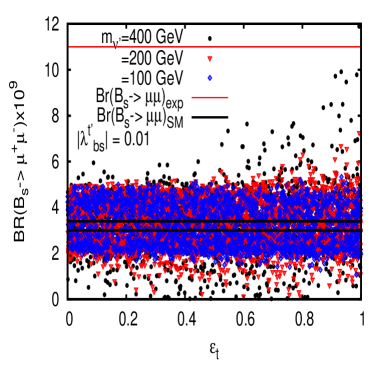
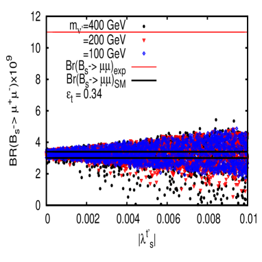
Figure 7: $BR(B_{s}\to\mu\mu)$ in the 4G2HDM from box diagrams with the $H^{+}$ and $(t,\nu^{\prime})$, $(t^{\prime},\nu^{\prime})$ exchanges, as a function of $\epsilon_{t}$ (fixing $\epsilon_{b}=0.01$) and $\lambda_{bs}^{t^{\prime}}\equiv V_{t^{\prime}b}V_{t^{\prime}s}^{\ast}$, for $m_{\nu^{\prime}}=100,~{}200,~{}400$ GeV, $m_{\tau^{\prime}}=m_{\nu^{\prime}}$ and $m_{H^{+}}=500$ GeV. We considered only values of $\delta_{U_{2}}$ and $\delta_{\Sigma_{2}}$ which are allowed by $a_{\mu}$ given in Eq. 5, keeping both of them $\lower 2.15277pt\hbox{$\>\buildrel<\over{\sim}\>$}0.2$. Also shown are the experimental 95% CL upper bound (upper/red horizontal line) and the SM predicted range ($1\sigma$) of values (lower/black horizontal lines).

In Fig. 7 we plot the contribution to $BR(B_{s}\to\mu\mu)$ in the 4G2HDM from the box diagrams with the $H^{+}$ and $(t,\nu^{\prime})$, $(t^{\prime},\nu^{\prime})$ exchanges, as a function of $\epsilon_{t}$ (fixing $\epsilon_{b}=0.01$) and $\lambda_{bs}^{t^{\prime}}\equiv V_{t^{\prime}b}V_{t^{\prime}s}^{\ast}$, for $m_{\nu^{\prime}}=100,~{}200,~{}400$ GeV, $m_{\tau^{\prime}}=m_{\nu^{\prime}}$ and $m_{H^{+}}=500$ GeV. The allowed ranges of the key parameters $\delta_{U_{2}}$ and $\delta_{\Sigma_{2}}$, which control the muon $g-2$ in our model, are randomly chosen in the range $[0,0.2]$ to be consistent with $a_{\mu}^{exp}$ given in Eq. 4. We also show the current experimental bound lhcb1 and the SM predicted value for $BR(B_{s}\to\mu\mu)$. We see that the contribution from the new (i.e., in the 4G2HDM) box diagrams that involve the heavy 4th generation neutrino is consistent with the current experimental bound on $BR(B_{s}\to\mu\mu)$ for values of $\delta_{U_{2}}$ and $\delta_{\Sigma_{2}}$ that reproduce the observed muon $g-2$. It is also interesting to note that both in the SM4 and in the 4G2HDM, Br$(B_{s}\to\mu^{+}\mu^{-})$ can differ from the SM value by at-most a factor of O(3) in either direction.

V Summary and discussion

We have considered the effects of 1-loop exchanges of heavy 4th generation leptons on the muon $g-2$, on the lepton flavor violating decays $\mu\to e\gamma$, $\tau\to\mu\gamma$ and on $B_{s}\to\mu^{+}\mu^{-}$, in the 4G2HDM which is a 2HDM where the Higgs doublet with the heavier VEV is coupled only to the 4th generation doublet while the “lighter” Higgs doublet is coupled to fermions of the 1st-3rd generations. This model is particularly motivated for the leptonic sector, as it effectively addresses the heaviness of a 4th generation EW-scale neutrino.

The muon $g-2$ is sensitive in our model to the product $\delta_{U_{2}}\cdot\delta_{\Sigma_{2}}$, where $\delta_{U_{2}}\equiv\frac{U_{24}^{*}}{U_{44}^{*}}$, $\delta_{\Sigma_{2}}\equiv\frac{\Sigma_{42}^{e*}}{\Sigma_{44}^{\nu}}$, $U_{ij}$ is the leptonic CKM-like PMNS matrix and $\Sigma_{ij}^{e},~{}\Sigma_{ij}^{\nu}$ are new mixing matrices in the charged and neutral leptonic sectors that are unique to the 4G2HDM.

We find that, depending on the mass $m_{\nu^{\prime}}$, the experimentally measured muon magnetic moment can be accounted for if ${\cal O}(10^{-3})\lower 2.15277pt\hbox{$\>\buildrel<\over{\sim}\>$}\delta_{U_{2}}\cdot\delta_{\Sigma_{2}}\lower 2.15277pt\hbox{$\>\buildrel<\over{\sim}\>$}{\cal O}(10^{-2})$. We also find that the decays $\mu\to e\gamma$ and $\tau\to\mu\gamma$ can have branching ratios which are not too far below the current bounds, i.e., of ${\cal O}({\rm few}\cdot 10^{-13})$ and ${\cal O}({\rm few}\cdot 10^{-9})$, respectively, if the products $\delta_{U_{1}}\cdot\delta_{\Sigma_{2}},~{}\delta_{U_{2}}\cdot\delta_{\Sigma_{1}}\sim{\cal O}(10^{-6})$ and $\delta_{U_{2}}\cdot\delta_{\Sigma_{3}},~{}\delta_{U_{3}}\cdot\delta_{\Sigma_{2}}\sim{\cal O}(10^{-3})$, respectively.

We also considered the effects of one-loop exchanges of the 4th generation heavy neutrino $\nu^{\prime}$ on the decay $B_{s}\to\mu^{+}\mu^{-}$ and found that, in the four generations model considered here, ${\rm BR}(B_{s}\to\mu^{+}\mu^{-})$ can be larger or smaller than the SM predicted value by a factor of about three, for values of ${\cal O}(10^{-3})\lower 2.15277pt\hbox{$\>\buildrel<\over{\sim}\>$}\delta_{U_{2}}\cdot\delta_{\Sigma_{2}}\lower 2.15277pt\hbox{$\>\buildrel<\over{\sim}\>$}{\cal O}(10^{-2})$, which render the observed value of the muon $g-2$ to be consistent with the current upper limit on this decay.

Acknowledgments: SBS acknowledges research support from the Technion. The work of AS was supported in part by the U.S. DOE contract #DE-AC02-98CH10886(BNL).

References

(1)
(2)
T. Kinoshita, M. Nio,
Phys. Rev. D70, 113001 (2004);
T. Kinoshita, M. Nio,
Phys. Rev. D73, 013003 (2006);
T. Kinoshita, M. Nio,
Phys. Rev. D73, 053007 (2006);
G. Gabrielse, D. Hanneke, T. Kinoshita, M. Nio, B. C. Odom,
Phys. Rev. Lett. 97, 030802 (2006);
T. Aoyama, M. Hayakawa, T. Kinoshita, M. Nio,
Phys. Rev. Lett. 99, 110406 (2007);
D. Hanneke, S. Fogwell, G. Gabrielse,
Phys. Rev. Lett. 100, 120801 (2008);
(3)
G. Degrassi, G. F. Giudice,
Phys. Rev. D58, 053007 (1998);
A. Czarnecki, W. J. Marciano, A. Vainshtein,
Phys. Rev. D67, 073006 (2003);
S. Heinemeyer, D. Stockinger, G. Weiglein,
Nucl. Phys. B699, 103-123 (2004);
T. Gribouk, A. Czarnecki,
Phys. Rev. D72, 053016 (2005);
(4)
J. Prades, E. de Rafael, A. Vainshtein,
In: Roberts, Lee B., Marciano, William J. (eds.):“Lepton dipole moments” 303-317, arXiv:0901.0306 [hep-ph];
M. Davier, A. Hoecker, G. Lopez Castro, B. Malaescu, X. H. Mo, G. Toledo Sanchez, P. Wang, C. Z. Yuan et al.,
Eur. Phys. J. C66, 127-136 (2010).
(5)
C. Bouchiat and L. Michel,
Phys. Rev. 106, 170 (1957);
M. Gourdin and E. De Rafael,
Nucl. Phys. B 10, 667 (1969).
(6)
M. Davier, A. Hoecker, B. Malaescu, C. Z. Yuan and Z. Zhang,
Eur. Phys. J. C 66, 1 (2010).
(7)
K. Hagiwara, A. D. Martin, D. Nomura and T. Teubner,
Phys. Lett. B 649, 173 (2007).
(8)
F. Jegerlehner and A. Nyffeler,
Phys. Rept. 477, 1 (2009).
A. Nyffeler,
Phys. Rev. D 79, 073012 (2009).
(9)
See pdg minireview on muon g-2 in http://pdglive.lbl.gov.
(10)
F. Jegerlehner and A. Nyffeler,
Phys. Rept. 477 (2009) 1;
For a recent update, see J. Prades, Acta Phys. Polon. Supp. 3, 75 (2010).
(11)
J. L. Lopez, D. V. Nanopoulos, X. Wang,
Phys. Rev. D49, 366-372 (1994);
U. Chattopadhyay, P. Nath,
Phys. Rev. D53, 1648-1657 (1996);
S. P. Martin, J. D. Wells,
Phys. Rev. D64, 035003 (2001).
(12)
S. Bar-Shalom, S. Nandi and A. Soni,
Phys. Rev. D 84, 053009 (2011)
(13) M.A. Luty, Phys. Rev. D41, 2893 (1990).
(14)
G. D. Kribs, T. Plehn, M. Spannowsky and T. M. P. Tait,
Phys. Rev. D 76, 075016 (2007);
M. S. Chanowitz,
Phys. Rev. D 79, 113008 (2009).
(15)
G. W. S. Hou,
arXiv:0810.3396 [hep-ph].
(16)
M. Hashimoto and V. A. Miransky, Phys. Rev. D81, 055014 (2010).
(17)
P. Q. Hung and C. Xiong, Phys. Lett. B694, 430 (2011).
(18) See e.g., A. Koryton (CMS collaboration), talk given at
the EPS-HEP 2011, July 21-27, Grenoble, France.
(19)
X.-G. He and G. Valencia, arXiv:1108.0222 [hep-ph].
(20)
A. Soni, A. K. Alok, A. Giri, R. Mohanta and S. Nandi,
Phys. Lett. B 683, 302 (2010).
(21)
A. Soni, A. K. Alok, A. Giri, R. Mohanta and S. Nandi,
Phys. Rev. D 82, 033009 (2010).
(22)
A. J. Buras, B. Duling, T. Feldmann, T. Heidsieck, C. Promberger and S. Recksiegel,
JHEP 1009, 106 (2010).
(23) W. S. Hou and C. Y. Ma, Phys. Rev. D82, 036002 (2010).
(24)
S. Nandi and A. Soni,
Phys. Rev. D 83, 114510 (2011)
(25)
See also,
M. Bobrowski, A. Lenz, J. Riedl and J. Rohrwild,
Phys. Rev. D 79, 113006 (2009);
O. Eberhardt, A. Lenz and J. Rohrwild,
Phys. Rev. D 82, 095006 (2010).
(26)
W. -S. Hou, F. -F. Lee, C. -Y. Ma,
Phys. Rev. D79, 073002 (2009).
(27)
J. P. Leveille,
Nucl. Phys. B137, 63 (1978).
(28) See e.g., G. Burdman, L. Da Rold, R. D’Elia Matheus, Phys. Rev. D82, 055015 (2010).
(29)
J. Adam et al. [MEG Collaboration],
Phys. Rev. Lett. 107, 171801 (2011).
(30)
M. Blanke, A. J. Buras, B. Duling, A. Poschenrieder, C. Tarantino,
JHEP 0705, 013 (2007).
(31)
M. Bona et al. (SuperB Collaboration),
arXiv:0709.0451 [hep-ex].
(32)
R. Aaij et al. (LHCb Collaboration),
Phys. Lett. B699, 330 (2011);
S. Chatrchyan et al. (CMS Collaboration),
arXiv:1107.5834 [hep-ex],
See also the public note LHCb-ANA-2011-039.
(33)
T. Aaltonen et al. (CDF Collaboration),
Phys. Rev. Lett. 107, 239903 (2011) and Phys. Rev. Lett. 107, 191801 (2011).
(34)
H. E. Logan and U. Nierste,
Nucl. Phys. B 586, 39 (2000).
(35)
G. Buchalla, A. J. Buras,
Nucl. Phys. B400, 225-239 (1993).
(36)
M. Misiak, J. Urban,
Phys. Lett. B451, 161-169 (1999).