An inertia ‘paradox’ for incompressible stratified Euler fluids

Abstract

The interplay between incompressibility and stratification can lead to non-conservation of horizontal momentum in the dynamics of a stably stratified incompressible Euler fluid filling an infinite horizontal channel between rigid upper and lower plates. Lack of conservation occurs even though in this configuration only vertical external forces act on the system. This apparent paradox was seemingly first noticed by Benjamin (J. Fluid Mech., vol. 165, 1986, pp. 445-474) in his classification of the invariants by symmetry groups with the Hamiltonian structure of the Euler equations in two dimensional settings, but it appears to have been largely ignored since. By working directly with the motion equations, the paradox is shown here to be a consequence of the rigid lid constraint coupling through incompressibility with the infinite inertia of the far ends of the channel, assumed to be at rest in hydrostatic equilibrium. Accordingly, when inertia is removed by eliminating the stratification, or, remarkably, by using the Boussinesq approximation of uniform density for the inertia terms, horizontal momentum conservation is recovered. This interplay between constraints, action at a distance by incompressibility, and inertia is illustrated by layer-averaged exact results, two-layer long-wave models, and direct numerical simulations of the incompressible Euler equations with smooth stratification.

1 Introduction

Among the many areas of classical mechanics, fluid dynamics arguably holds a special distinction for being a rich source of the sort of paradoxes that often arise from simplifying limit assumptions. Thus, for instance, the limit of zero viscosity gives rise to D’Alembert’s paradox on the drag experienced by rigid bodies moving in ideal fluids, while the opposite limit of dominating viscous stresses leads to the Stokes or Whitehead paradoxes of unphysical divergences for the same problem.

This work focuses on an effect that could also be viewed as paradoxical: horizontal momentum conservation is violated in the dynamics of a stratified ideal fluid filling an infinite horizontal channel between rigid bottom and lid boundaries, starting from localized initial conditions, even though the only external forces acting on the system are vertical (gravity and constraint forces from the horizontal boundary) and the fluid is free to move laterally. Of course, even for an inviscid fluid, lateral boundaries could lead to horizontal forces by action-reaction mechanisms due to the constrained motion, and so horizontal momentum conservation cannot in general be expected to hold for a stratified Euler fluid filling a finite domain enclosed by a rigid boundary. However, we shall see below that for a domain extending horizontally to infinity the infinite inertia possessed by the far fluid at rest acts as an effective lateral boundary, giving rise to violation of horizontal momentum conservation. While stratification is necessary for creating the relative inertia of the lateral fluid at rest, a subtlety of this effect is that incompressibility is also required to transmit forces arising from finite-range motion instantaneously all the way to infinity. Accordingly, the “light-cone” provided by the maximum speed of propagation of internal baroclinic modes gives a rough estimate of the boundary of the exterior region that can be considered as contributing to an effective-wall lateral confinement.

To the best of our knowledge, this limiting behaviour in the dynamics of a stratified fluid has not been given much attention in the literature. Benjamin (1986) appears to be the first to point out this curious property, in the course of his investigation on symmetries and Hamiltonian structures of the stratified, incompressible two–dimensional Euler equations. In particular, Benjamin shows that the invariant generally associated with translational symmetry is the fluid’s impulse rather than its momentum.

This Hamiltonian approach is compact and elegant, and its applications certainly deserve further study. Nonetheless, the physical mechanisms responsible for the dynamics seem to be more transparent by a direct approach with the simplest configuration of a two-layer fluid. This configuration has the added advantage of leading naturally into reliable models when long-wave asymptotics applies. A further advantage of the direct approach is that it can be immediately extended to three-dimensional settings for fluid domains between horizontal rigid planes. Admittedly, the effect considered here can be viewed as small, because momentum conservation is recovered as the size $\Delta\rho$ of the density range (which in practical cases such as water stratified with heat or salt, is typically $\Delta\rho/\rho\simeq 10^{-2}$)vanishes. Of course, the effect also relies on the abstract setup of infinite rigid bounding surfaces. Nonetheless, we think that this limiting case is of conceptual importance for a proper understanding of the dynamics of the incompressible limit for density-stratified fluids.

The paper is organized as follows. In §2 we first derive balance laws that imply the paradox for incompressible stratified Euler equations in an infinite channel, without approximations. Next, we show that the paradox remains in a two-layer fluid in the hydrostatic (dispersionless) non-Boussinesq approximation. In this simpler setting an explicit formula for the interface pressure can be derived. In §3, we show how the paradox can arise via direct numerical simulations of stratified incompressible Euler equations.

2 Layer averaged Euler equations

While the inertia effects that we focus upon here arise with general smooth stratifications, we work first with two-layer fluids. This setup is the most convenient for developing long-wave models, which can further illustrate the inertia effect by allowing explicit formulae to be derived. Similarly, the restriction to a single horizontal dimension is not essential, and our conclusions (and formalism) work for the full three-dimensional case of a horizontal fluid between infinite top and bottom rigid bounding plates. We choose to work with layer-averaged equations, which of course can be formulated independently of the assumption of stacked homogeneous layer stratification.

The dynamics of an inviscid and incompressible fluid stratified in layers of uniform density $\rho_{j}$ is governed by the Euler equations for the velocity components $(u_{j},w_{j})$ and the pressure $p_{j}$, in two dimensional Cartesian coordinates $(x,z)$,

$${u_{j}}_{x}+{w_{j}}_{z} = 0,$$ (1)

$${u_{j}}_{t}+u_{j}{u_{j}}_{x}+w_{j}{u_{j}}_{z} = -{p_{j}}_{x}/\rho_{j},$$ (2)

$${w_{j}}_{t}+u_{j}{w_{j}}_{x}+w_{j}{w_{j}}_{z} = -{p_{j}}_{z}/\rho_{j}-g,$$ (3)

where $g$ is the gravitational acceleration and subscripts with respect to space and time represent partial differentiation. In a two-fluid system, $j=1$ ($j=2$) stands for the upper (lower) fluid, and $\rho_{1}\leq\rho_{2}$ must be assumed for stable stratification.

For a channel with upper and lower rigid surfaces (see figure 1a for the setup and relevant notation) the kinematic boundary conditions are

$$w_{1}(x,{h_{1}},t)=0\,,\qquad w_{2}(x,-{h_{2}},t)=0\,,$$ (4)

where ${h_{1}}$ (${h_{2}}$) is the undisturbed thickness of the upper (lower) fluid layer, respectively. The boundary conditions at the interface $z={\zeta}(x,t)$ are the continuity of normal velocity and pressure

$${\zeta}_{t}+u_{1}{\zeta}_{x}=w_{1},\quad{\zeta}_{t}+u_{2}{\zeta}_{x}=w_{2},\quad p_{1}=p_{2}\equiv P\qquad{\rm at}\quad z={\zeta}(x,t),$$ (5)

where ${\zeta}(x,t)$ is the displacement of the interface from the equilibrium configuration surface $z=0$ and $P(x,t)$ denotes the interfacial pressure.

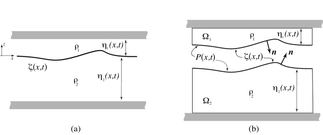
Figure 1: (a) Two-layer fluid setup and relevant notation. (b) The domains for computation of momentum balance

As to the lateral boundary conditions, a set of particular interest physically is the one that corresponds to localized initial data, i.e., the fluid is quiescent at infinity. This would require

$$\zeta(x,\cdot)\to 0\,,\quad{\mbox{\boldmath{$u$}}}_{j}(x,\cdot,\cdot)\to 0\,,\quad j=1,2\,,\qquad\hbox{as}\quad|x|\to\infty\,,$$ (6)

sufficiently fast, which in turn implies that at infinity hydrostatic equilibrium applies,

$${p_{j}}_{z}+\rho_{j}g=0,\quad j=1,2\,,\qquad\Rightarrow\qquad p_{j}=-g\rho_{j}z+P\,,\qquad\hbox{as}\quad|x|\to\infty\,.$$ (7)

In what follows we rewrite the Euler system (3) in terms of layer averages (see e.g. Wu 1981). (For a smoothly stratified fluid, this is equivalent to singling out an intermediate level set of constant density $z=\zeta(x,t)$ and carrying similar manipulations since such a set will always be a material surface.) We define the layer-mean quantities $\bar{f}$ as

$$\bar{f}(x,t)\equiv{1\over\eta_{j}}\int_{[\eta_{j}]}f(x,z,t){\rm d}z\,,$$ (8)

where $\eta_{j}$ are the layer thicknesses $\eta_{i}\equiv h_{j}+(-1)^{j}\zeta$, and, abusing notation a little by not differentiating overbars with respect to lower or upper layer, the intervals of integration $[\eta_{j}]$ are $z\in(\zeta,h_{1})$ for the upper and $z\in(-h_{2},\zeta)$ for the lower layers, respectively. Vertically integrating (1)–(2) across the layers and imposing the boundary conditions (4)–(5) yields the layer-mean equations for the upper (lower) fluid

$${\eta_{j}}_{t}+\big{(}\eta_{j}{{\overline{u}_{j}}}\big{)}_{x} =0,$$ (9)

$$\rho_{j}(\eta_{j}{{\overline{u}_{j}}})_{t}+\rho_{j}\big{(}\eta_{j}\overline{{u_{j}}{u_{j}}}\big{)}_{x} =-(\eta_{j}\overline{{p_{j}}})_{x}+(-1)^{j}{\zeta}_{x}P\,,\qquad j=1,2\,.$$ (10)

(We use the notation $\overline{{u_{j}}{u_{j}}}$ here and in similar formulae below instead of the equivalent $\overline{{u_{j}}^{2}}$ because the latter applies only to the two dimensional case, whereas the former can be used for three dimensions as well, upon interpreting the horizontal velocity product as a two-tensor and replacing the $x$-derivative by a divergence over the horizontal variables.)

For incompressible, inviscid fluids under a body-force density $\mbox{\boldmath{$f$}}(\mbox{\boldmath{$x$}},t)$ in a domain $\Omega$, the momentum balance in Eulerian form is expressed by

$${d\mbox{\boldmath{$\Pi$}}\over dt}\equiv{d\over dt}\int_{\Omega}\rho\mbox{\boldmath{$u$}}\,dV=\int_{\Omega}{\partial\over\partial t}(\rho\mbox{\boldmath{$u$}})\,dV+\int_{\Omega}\hbox{div}(\rho\mbox{\boldmath{$u$}}\mbox{\boldmath{$u$}})\,dV=-\int_{\partial\Omega}p\mbox{\boldmath{$n$}}\,dA\,+\,\int_{\Omega}\rho\mbox{\boldmath{$f$}}\,dV\,,$$ (11)

where $n$ is the outward normal to the surface $\partial\Omega$, and $dV$, $dA$ denote the volume and area elements, respectively. Layer averages are just a local version of the integral form of the horizontal momentum balance for each layer (see figure 1b), which can be expressed by integrating equations (10) over some $x$-interval $L_{-}\leq x\leq L_{+}$. We have

$${d{\Pi_{1}}_{j}\over dt}\equiv{d\over dt}\int_{L_{-}}^{L_{+}}\rho_{j}\eta_{j}{{\overline{u}_{j}}}\,dx+\left.\rho_{j}\eta_{j}\overline{{u_{j}}{u_{j}}}\right|_{L_{-}}^{L_{+}}=-\left.\eta_{j}\overline{{p_{j}}}\right|_{L_{-}}^{L_{+}}+(-1)^{j}\int_{L_{-}}^{L_{+}}\zeta_{x}P\,dx\,,$$ (12)

for the upper ($j=1$) and lower ($j=2$) layer respectively, since the outward normals along the interface are $\mbox{\boldmath{$n$}}\propto(\pm\zeta_{x},1)$, and neither the pressure at the rigid horizontal surfaces or the external gravity field contribute horizontal components of forces.

In hydrostatic equilibrium, the layer-mean pressures are

$$\overline{{p_{j}}}=(-1)^{j}g\rho_{j}{\eta_{j}\over 2}+P\,,\quad j=1,2\,.$$ (13)

Hence, by a suitable definition of the limit procedure $L_{\pm}\to\pm\infty$, the lateral equilibrium boundary conditions imply that for each infinite upper and lower layer the horizontal momenta are conserved if and only if

$$-h_{1}\left.P\right|_{-\infty}^{+\infty}-\int_{-\infty}^{+\infty}\zeta_{x}P\,dx=0\,,\qquad-h_{2}\left.P\right|_{-\infty}^{+\infty}+\int_{-\infty}^{+\infty}\zeta_{x}P\,dx=0\,,$$ (14)

at all times, that is, if

$$\int_{-\infty}^{+\infty}\zeta_{x}P\,dx=0\qquad\hbox{and}\qquad\left.P\right|_{-\infty}^{+\infty}=0\,.$$ (15)

(These relations are precisely the ones encountered in the study of single-layer fluids when an external pressure distribution is applied to their free surface.)

Summing up the two momentum equations (10) (for $j=1,2$) yields the mean layer balance law for the total momentum of the fluid

$$\partial_{t}\Big{(}\rho_{1}({{\eta}_{1}}{{\overline{u}_{1}}})+\rho_{2}({{\eta}_{2}}{{\overline{u}_{2}}})\Big{)}=-\partial_{x}\Big{(}\rho_{1}\big{(}{{\eta}_{1}}\overline{{u_{1}}{u_{1}}}\big{)}+\rho_{2}\big{(}{{\eta}_{2}}\overline{{u_{2}}{u_{2}}}\big{)}+{{\eta}_{1}}\overline{{p_{1}}}+{{\eta}_{2}}\overline{{p_{2}}}\Big{)}\,.$$ (16)

By action and reaction the contribution from the pressure at the interface $P(x,t)$ drops from the balance (16) as well as from the integral version of the total horizontal momentum. Thus, the condition for total momentum conservation is that $\left.P\right|_{-\infty}^{+\infty}=0$, since (13) with (12) in this limit yields

$${d\Pi_{1}\over dt}={d{\Pi_{1}}_{1}\over dt}+{d{\Pi_{1}}_{2}\over dt}=-(h_{1}+h_{2})\left.P\right|_{-\infty}^{+\infty}\,.$$

At first sight, for localized displacements and velocities, it might not be clear how the asymptotic values of the interfacial pressure could be different from plus to minus infinity, as the hydrostatic equilibrium is identical at both ends and the interfacial pressure simply keeps track of the overall constant of integration up to which pressure is defined. For a free upper surface, this constant is usually set by the atmospheric pressure; if this is assumed to be uniform, no pressure jump can occur. However, a system with a rigid lid is constrained, and reaction forces can develop in response to the constraint. Thus, we now focus on the consequences of the rigid lid constraint $\eta_{1}+\eta_{2}=h_{1}+h_{2}$. The continuity equations (9) imply

$$\big{(}\eta_{1}{{\overline{u}_{1}}}+\eta_{2}{{\overline{u}_{2}}}\big{)}_{x}=0\quad\Rightarrow\quad\eta_{1}{{\overline{u}_{1}}}+\eta_{2}{{\overline{u}_{2}}}\equiv Q(t)\,,$$ (17)

that is, the volume flux $Q$ through the channel can only be a function of time. Dividing the momentum equations (10) by the respective densities and summing the resulting equations yields

$$\partial_{x}\Big{(}{{\eta}_{1}}\overline{{u_{1}}{u_{1}}}+{{\eta}_{2}}\overline{{u_{2}}{u_{2}}}+{1\over\rho_{1}}{{\eta}_{1}}\overline{{p_{1}}}+{1\over\rho_{2}}{{\eta}_{2}}\overline{{p_{2}}}\Big{)}=\Big{(}{1\over\rho_{2}}-{1\over\rho_{1}}\Big{)}\zeta_{x}P-\dot{Q}\,.$$ (18)

With the far-field zero boundary conditions on the velocities, which implies $Q(t)=0$ at all times, equation (18) can be interpreted as an expression that determines the (unknown) interfacial pressure $P(x,t)$ in terms of the divergence of the layer-mean quantities. By integrating in $x$ and taking into account the boundary conditions (6)-(7) we obtain

$$\Big{(}{h_{2}\over\rho_{2}}+{h_{1}\over\rho_{1}}\Big{)}\left.P\right|_{-\infty}^{+\infty}=\Big{(}{1\over\rho_{2}}-{1\over\rho_{1}}\Big{)}\int_{-\infty}^{+\infty}\zeta_{x}P\,dx\,,$$ (19)

which shows that unless the surface integral of the pressure along the interface at the right-hand-side of (19) vanishes, or the layers have the same density, the extremal values of the interfacial pressure will in general be different. The equivalent expression

$$\rho_{2}\Big{(}h_{1}\left.P\right|_{-\infty}^{+\infty}+\int_{-\infty}^{+\infty}\zeta_{x}P\,dx\Big{)}=-\rho_{1}\Big{(}h_{2}\left.P\right|_{-\infty}^{+\infty}-\int_{-\infty}^{+\infty}\zeta_{x}P\,dx\Big{)}\,$$

shows that if one of the two conditions in (14) is satisfied, i.e., horizontal momentum of one of the layers is conserved, the other will be as well, as the surface pressure integral is linked to the difference of asymptotic interfacial pressure by the rigid lid constraint. Thus, conservation of the horizontal momentum of just one of the two layers implies conservation of the total horizontal momentum of the fluid. On the other hand, with nonzero surface pressure integral along the interface total horizontal momentum will change with time, i.e., the bulk of the fluid will in general undergo accelerations. Horizontal momentum is always conserved if the fluid is homogeneous, $\rho_{1}=\rho_{2}$, as (19) shows that in this case interfacial pressure forces cannot add up to provide a total pressure gradient between the far ends of the channel. Perhaps more notable is the effect of the Boussinesq approximation of taking $\rho_{1}=\rho_{2}$ in front of the inertial terms (cf. Boonkasame & Milewski, 2011 for an analysis of the interplay between interfacial pressure and flux in the non-Boussinesq case and of the stability properties of the long-wave regime). Just as in the case of homogeneous-density fluid, build-up of pressure jump $\left.P\right|_{-\infty}^{+\infty}$ from interfacial pressure cannot occur in this case: taking the Boussinesq approximation in, e.g., equation (16), and applying the constraint $Q(t)=0$ sets the right-hand side of that equation to zero, so that $\dot{\Pi}_{1}=0$, which in turn implies $\left.P\right|_{-\infty}^{+\infty}=0$. Hence total as well as individual layer momenta are always conserved in the Boussinesq approximation for two-layer channel flows with far-field hydrostatic equilibrium boundary conditions.

It remains to be seen if states of the fluid leading to a nonzero interfacial integral at the right-hand of equation (19) can develop during the evolution governed by the Euler equations (even for a general smoothly stratified fluid). A convenient starting point is offered by a choice of initial conditions corresponding to zero velocity and a local deformation of density level sets away from the (flat) ones for hydrostatic equilibrium. This is the choice of initial data used in the numerical simulations below, where in particular we take $x$-antisymmetric initial deformations. As we will see, during the subsequent evolution, this choice leads to an analogue for a finite domain of time variation of horizontal momentum for the infinite channel. The numerical simulations will be performed with near-two-layer configurations, and with initial data which are slowly varying in $x$. For such a case explicit expressions (not readily available in the general case) for the quantities in equation (19) can be derived approximately using long-wave asymptotics.

2.1 Shallow water models

At leading order in a long-wave asymptotic expansion (see e.g. Yih, 1980), the hydrostatic approximation for the pressures holds throughout the fluid domain, not just as far-field boundary conditions. This can be used to derive a closed form expression for the interfacial pressure in equation (18). The result is expressed in terms of well known two-layer (five-equation, dispersionless) shallow-water model (see e.g. [Milewski et al. 2004]). We have

$$\partial_{x}\Big{(}{{\eta}_{1}}\overline{{u_{1}}{u_{1}}}+{{\eta}_{2}}\overline{{u_{2}}{u_{2}}}+g\zeta(h_{1}+h_{2})+g{h^{2}_{2}-h_{1}^{2}\over 2}+\Big{(}{\eta_{1}\over\rho_{1}}+{\eta_{2}\over\rho_{2}}\Big{)}P\Big{)}=\zeta_{x}\Big{(}{1\over\rho_{2}}-{1\over\rho_{1}}\Big{)}P\,,$$

so that, with the identities $\zeta_{x}=-{\eta_{1}}_{x}={\eta_{2}}_{x}$ used in the right-hand side of this expression,

$$\partial_{x}\big{(}{{\eta}_{1}}\overline{{u_{1}}{u_{1}}}+{{\eta}_{2}}\overline{{u_{2}}{u_{2}}}+g\zeta(h_{1}+h_{2})\big{)}=-P_{x}\Big{(}{\eta_{1}\over\rho_{1}}+{\eta_{2}\over\rho_{2}}\Big{)}\,.$$

Upon splitting the average of products into the products of averages, this coincides with the expression derived from the five-equation model, and yields

$$\left.P\right|_{-\infty}^{+\infty}=-{\rho_{1}\rho_{2}}\int_{-\infty}^{\infty}{({{\eta}_{1}}\overline{{u_{1}}}^{2}+{{\eta}_{2}}\overline{{u_{2}}}^{2})_{x}\over\rho_{1}\eta_{2}+\rho_{2}\eta_{1}}dx\,.$$ (20)

Here a term with the factor $g(h_{1}+h_{2})\zeta_{x}$ has been dropped because the denominator is only a (linear) function of $\zeta$ thus making the ratio a perfect $x$-derivative, vanishing when the boundary conditions on $\zeta$ are applied. Thus, at leading order total horizontal momentum conservation requires the extra constraint on the choice of initial data that make the above integral vanish, which is manifestly not satisfied for general functions $\overline{u}_{j}$ and $\eta_{j}$. Note that if $\rho_{1}=\rho_{2}$ the denominator in the integrand in (20) becomes a constant, making the integral null on account of the velocity boundary conditions.

Finally, we remark that equation (20) shows that the symmetries of the system with respect to the horizontal variable allow the identification of a large class of solutions compatible with momentum conservation (in the hydrostatic approximation). Indeed, it is easy to check that if initially $\eta_{1}$, $\eta_{2}$ are even functions and $\overline{u}_{1}$, $\overline{u}_{2}$ are odd functions with respect to $x$, then these symmetries are preserved by the evolution of the system. For such solutions, (20) shows that the (null) horizontal momentum is conserved. However, generic initial conditions not in this class can be shown to evolve to non-zero $\left.P\right|_{-\infty}^{+\infty}$, even starting from null values of this pressure jump, or, remarkably, even when the velocities are chosen to be initially zero. For this latter case, this can be seen by looking at the higher order dispersive (non-hydrostatic) corrections to the shallow-water model as reported in Choi & Camassa (1999). At $t=0$ with zero initial velocities these corrections modify equation (20) as

$$\left.P\right|_{-\infty}^{+\infty}=\frac{1}{3}\int_{-\infty}^{+\infty}\frac{\left(\eta_{1}^{3}{{{\overline{u}_{1}}}}_{xt}+\eta_{2}^{3}{{{\overline{u}_{2}}}}_{xt}\right)_{x}}{\eta_{1}/\rho_{1}+\eta_{2}/\rho_{2}}\ dx\,,$$ (21)

which, by bringing into the integrand the time-derivatives of the velocities shows that the pressure jump can be non-zero even if the velocities are initially zero. In particular, antisymmetric initial displacements of the interface can lead to non-zero $P{|}_{-\infty}^{+\infty}$, whereas this pressure jump always vanishes for symmetric initial data.

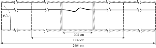
Figure 2: Sketch of the fluid test domain and its symmetrical padding by wings of increasing length, doubling and quadrupling the period as shown.

3 Numerical simulations

The above discussion was conducted with laterally unbounded domains in mind. Of course, such an idealization cannot be used either in reality or in numerical studies. However, in this section we provide numerical evidence that the effective-wall lateral confinement, and hence non-conservation of horizontal momentum, can occur in finite domains, due to the relative inertia of a stratified, incompressible Euler fluid. First, we remark that, for domains bounded by rigid lateral walls, the finite-domain version of equation (19) (obtained by writing $\pm L/2$ in place of $\pm\infty$) continues to hold; in the limit of the walls moving to infinity we simply recover the hydrostatic balance as expressed by (19). Next, consider the case of periodic boundary conditions in the periodic box $[-L/2,L/2]$. This requires $\left.P\right|_{-L/2}^{+L/2}=0$ and hence the horizontal momentum for the whole periodic domain is conserved. We focus on a subset of the fluid domain, henceforth referred to as the “test section,” obtained by taking a (much) smaller interval embedded in the period (cf. figure 2). Within this test section, we apply localized initial conditions for velocity and pycnocline displacement, e.g., by requiring that the data have compact support on a small subset of the test section’s region. The analogue of equation  (19) for a periodic domain becomes an equation for the flux $Q$,

$$L\dot{Q}=\left(\frac{1}{\rho_{2}}-\frac{1}{\rho_{1}}\right)\int_{-L/2}^{L/2}\zeta_{x}P\ dx.$$ (22)

Consider the limit $L\to\infty$ of this equation. For definiteness, let $\zeta$ be a function with compact support and suppose that all the velocities are zero at $t=0$. The integral on the right-hand side will be bounded as $L\to\infty$ (assuming that $P$ remains bounded on finite domains), so that $\dot{Q}\sim L^{-1}$. Suppose the test section extends from $-A/2$ to $A/2$ and $\mathrm{supp}(\zeta)\subset[-A/2,A/2]$. At $t=0$, after integrating (18) in the test section and eliminating $\dot{Q}$, we obtain

$$\left(\frac{1}{\rho_{2}}-\frac{1}{\rho_{1}}\right)\left(1-\frac{A}{L}\right)\int_{\mathrm{supp}(\zeta)}\zeta_{x}P\ dx=\left(\frac{h_{2}}{\rho_{2}}+\frac{h_{1}}{\rho_{1}}\right)P\Big{|}_{-A/2}^{+A/2}\,.$$ (23)

If we extend the test section to infinity with the double scaling limit $A,L\to\infty$ and $A/L\to 0$, the previous formula becomes (19). Though valid only at time $t=0$, this argument shows how the limit of infinite period for localized initial data can agree with the pressure differential of the infinite channel in hydrostatic balance at infinity.

We now explore numerically the time evolution of localized initial data under both periodic and rigid (impermeable) wall boundary conditions. In particular, we first compute the evolution of the flux $Q(t)$ and horizontal momentum $\Pi_{1}(t)$ for the test section alone. We then compare the resulting time series with those from simulations from the same initial conditions in progressively longer channels under periodic boundary conditions, see figure 2. Thus, while the total horizontal momentum for these longer periodic channels is conserved, that computed only in the embedded test-section will in general exhibit time dependence. Owing to the added inertia of the “padding” wings bracketing the test section in the longer channels, we expect this time dependence to show some similarity with that of the walled-in test section. That is, the added inertia acts as virtual walls, which could then approximate actual walls in the limit of an infinite periodic channel.

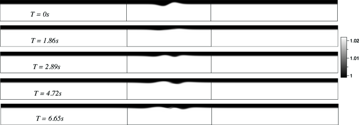
Figure 3: Density field from the numerical simulation of the evolution from the initial data in the 1232 cm long tank with the center 308 cm test section marked by the vertical lines.

The details of our numerical simulations are as follows. The initial conditions in all our simulations (all performed using dimensional quantities, and translating the origin of the coordinates to the bottom) are chosen to be the antisymmetric interface displacement through $\zeta_{0}(x)=h_{2}+{x/2}\exp(-{x^{2}/\sigma^{2}})$ together with zero initial velocities. This function displaces the smooth equilibrium density function $\rho_{e}(z)$ to give the initial condition $\rho_{0}$ (with obvious meaning of notation)

$$\rho_{0}(x,z)=\rho_{1}+{\rho_{2}-\rho_{1}\over 2}\left(1+\tanh\left[{\gamma}(\zeta_{0}(x)-z)\right]\right)\,,\qquad z\in[0\,,H]\,.$$ (24)

Here, $\sigma=30$ cm, $\rho_{1}=0.999$ g/cm³, $\rho_{2}=1.022$ g/cm³, $H=77$ cm, $h_{2}=62$ cm, and the thickness of the pycnocline (defined as the distance between density isolines corresponding to $10$% and $90$% of the total density jump) is set by the parameter $\gamma=0.5$ to correspond to about $4.5$ cm (all of these parameters are suggested by those typical for experiments with salt-stratified water). Notice that this choice of parameters gives effectively an initial condition of compact support, with the initial departure from hydrostatic equilibrium for $|\rho-\rho_{e}|/\rho_{e}$ of order $10^{-10}$ at the boundary of the test section $x=\pm 154$ cm; this departure remains below $10^{-7}$ in all our runs. The simulations (see figure 3) are performed using the numerical code VARDEN which solves the stratified incompressible Euler equations (for details see [Almgren et al. 1998].) We typically use a square grid with $512$ points along the vertical, although we have run cases with doubled and half this resolution to assess convergence. Figure 4a shows the time series of the horizontal momentum of the test section for the walled-in configuration, and compares it to that computed with periodic boundary conditions with quadrupled and octupled periodic extensions. As can be seen, there is indeed a tendency for the longer channel to yield a momentum evolution closer to that of the walled section, for the initial (short) time displayed. As expected, later time evolution shows larger discrepancies but still with similar overall behavior and magnitudes. This is in rough agreement with the estimate from the fastest baroclinic wave speeds, which for this parameter choice are of order $16$ cm/s, and with the horizontal scale of the initial condition with respect to that of the test section. For reference, we remark that the code maintains the total horizontal momentum for the periodic channels close to zero (the initial value) with an error of order $10^{-3}$. Figure 4b presents the time series of the flux $Q(t)$ for the same runs. The flux is computed at different $x$-locations, yielding the same value to within a relative error of $10^{-10}$ (thus further validating the convergence of the code). As can be seen by the different curves, the flux appears to scale as the inverse of the channel length $L$, in agreement with expression (22) for its initial time derivative. This can be taken as further evidence of the inertia provided by the padding wings (growing as $L$) which acts to oppose the fluid flux (recall that in the limit of an unbounded domain $Q\equiv 0$ due to the equilibrium at infinity).

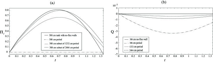
Figure 4: (a) Horizontal momentum time evolutions for the test section embedded in progressively larger periodic domains, starting from the same initial condition. The solid line correspond to the rigid wall boundaries. (b) Time series of fluxes $Q(t)$ with respect to increasing period $L$, for the same cases as (a). The flux decreases as $1/L$ in response to the larger inertia of the channel “padding” wings.

The inverse scaling with $L$ can be given further analytic interpretation. In fact, the analogue of (20) for the leading-order hydrostatic (and hence dispersionless) long-wave approximation is

$$\dot{Q}\int_{-L/2}^{+L/2}{1\over\eta_{1}/\rho_{1}+\eta_{2}/\rho_{2}}\,dx+\int_{-L/2}^{+L/2}{(\eta_{1}\overline{u_{1}}^{2}+\eta_{2}\overline{u_{2}}^{2})_{x}\over\eta_{1}/\rho_{1}+\eta_{2}/\rho_{2}}\,dx=0\,.$$ (25)

For zero-velocity initial conditions, this expression yields $\dot{Q}(0)=0$, in contrast to the time series depicted in figure 4b. This discrepancy brings forth a limitation of the hydrostatic (and hence dispersionless) long-wave model. It is generally accepted that the dispersionless approximation works well at intermediate times, while at long times the system could display a gradient catastrophe, which can be avoided by restoring dispersive effects (Esler and Pearce, 2011). Remarkably, equation (25) shows that dispersive effects can also be qualitatively relevant at short times, even in the absence of large $x$-derivatives. Specifically, at $t=0$ with zero initial velocities the dispersive terms turn (25) into

$$\int_{-L/2}^{+L/2}\frac{-\dot{Q}(0)+\frac{1}{3}\left(\eta_{1}^{3}{{{\overline{u}_{1}}}}_{xt}+\eta_{2}^{3}{{{\overline{u}_{2}}}}_{xt}\right)_{x}}{\eta_{1}/\rho_{1}+\eta_{2}/\rho_{2}}\ dx=0.$$ (26)

By computing the leading-order long-wave asymptotic expressions for the time derivatives (Choi & Camassa, 1999) in equation (26), the initial slope of the flux turns out to be

$$\dot{Q}(0)=\left(\int_{-L/2}^{+L/2}\frac{B_{x}}{\eta_{1}/\rho_{1}+\eta_{2}/\rho_{2}}\ dx\right)\left(\int_{-L/2}^{+L/2}\frac{1-A_{x}}{\eta_{1}/\rho_{1}+\eta_{2}/\rho_{2}}\ dx\right)^{-1},\,\text{where}$$

$$A=\frac{\eta_{1}^{3}}{3}\Big{(}\frac{\rho_{2}}{\eta_{2}\rho_{1}+\eta_{1}\rho_{2}}\Big{)}_{x}+(1\leftrightarrow 2),\quad B=\frac{g(\rho_{2}-\rho_{1})\eta_{1}^{3}}{3}\Big{(}\frac{\eta_{2}{\eta_{2}}_{x}}{\eta_{2}\rho_{1}+\eta_{1}\rho_{2}}\Big{)}_{x}-(1\leftrightarrow 2)\,.$$

Even within this leading-order approximation, there is rough agreement (in particular by capturing the correct sign) with the numerical data in figure 4b. This can also be seen as an a posteriori check on the robustness of the two-layer model. For instance, the theoretical prediction (adjusting for smooth stratification, as in Camassa & Tiron, 2011) is $\dot{Q}(0)\simeq-8.1\times 10^{-3}$ cm²/s² for the case in figure 4b with $L=1232$ cm, whereas the numerical result is $\dot{Q}(0)\simeq-1.9\times 10^{-3}$ cm²/s². Finally, we remark that the inertia effects can be further magnified by taking larger density variations. We have carried out tests with various density ratios, e.g., for $\rho_{2}=2\rho_{1}$ and $\rho_{2}=1.022$ g/cm³ the model predicts $\dot{Q}(0)\simeq-9.62$ cm²/s², while the measured numerical value is $\dot{Q}(0)\simeq-2.04$ cm²/s².

References

- [Almgren et al. 1998] Almgren A. S., Bell J. B., Colella P., Howell L. H., & Welcome M.L. 1998 A conservative adaptive projection method for the variable density incompressible Navier-Stokes equations. J. Comp. Phys., 142, 1–46.
- [Benjamin 1966] Benjamin T. B. 1966 Internal waves of finite amplitude and permanent form. J. Fluid Mech., 25, 241–270.
- [Benjamin 1986] Benjamin T. B. 1986 On the Boussinesq model for two-dimensional wave motions in heterogeneous fluids. J. Fluid Mech., 165, 445–474.
- [Milewski et al. 2011] Boonkasame A. & Milewski P. 2011 The stability of large-amplitude shallow interfacial non-Boussinesq flows. Stud. Appl. Math., DOI: 10.1111/j.1467-9590.2011.00528.x.
- [Camassa & Tiron 2011] Camassa R. & Tiron R. 2011 Optimal two-layer approximation for continuous density stratification. J. Fluid Mech., 669, 32–54.
- [Choi & Camassa 1999] Choi W. & Camassa R. 1999 Fully nonlinear internal waves in a two-fluid system. J. Fluid Mech., 396, 1–36.
- [Esler and Pearce 2011] Esler J. G. & Pearce J. D. 2011 Dispersive dam-break and lock-exchange flows in a two-layer fluid. J. Fluid Mech., 667, 555–585.
- [Milewski et al. 2004] Milewski P., Tabak E., Turner C., Rosales R.R., & Mezanque F. 2004 Nonlinear stability of two-layer flows. Comm. Math. Sci., 2, 427–442.
- [Wu 1981] Wu, T.Y. 1981 Long waves in ocean and coastal waters. J. of Eng. Mech., 107, 501–522.
- [Yih 1980] Yih C. Stratified Flows, Academic Press, New York, 1980.